Submitted:
19 May 2025
Posted:
20 May 2025
Read the latest preprint version here
Abstract
In information systems, data analysis plays a crucial role in uncovering hidden patterns and insights. Visualizing data behavior enables researchers to examine its dynamics, strengths, and limitations.
For pure mathematical problems, traditional approaches rely on mathematical tools for problem-solving. However, adopting a data-driven approach---where relevant data is generated within the problem's scope and analyzed intuitively---allows for alternative perspectives and solutions.
In this article, we present an analytical and visual framework for addressing mathematical and engineering problems. By developing a novel manifold learning-based algorithm, we examine these problems from a unique perspective.
We demonstrate the effectiveness of this approach through various applications, including approximate solutions to partial differential equations (PDEs) and classical mathematical problems such as studying the distribution and behavior of prime numbers. Our results show that even pure mathematical problems can benefit from this methodology.
This framework can also be applied to other scientific and engineering disciplines. We aim to provide innovative perspectives on diverse challenges across mathematics, engineering, and the sciences.
Keywords:
manifold learning
; data-driven analysis
; PDEs
; prime number distribution
; visual analytics
; scientific computing
1. Introduction
Visual observation of the behavior of data and their associated functions can reveal various behavioral aspects, highlighting ambiguous points and deviations from the goals defined in the objective function. This process often leads to the discovery of new solutions or specific areas of interest within the existing data [1].
Manifold learning spans multiple disciplines, including geometry, computation, and statistics, and has emerged as a significant research topic in data mining and statistical learning [2]. In simple terms, manifold learning refers to a class of algorithms designed to extract low-dimensional manifolds embedded within high-dimensional spaces [3]. Among the most popular linear dimensionality reduction techniques are Principal Component Analysis (PCA), which creates uncorrelated linear projections of data with maximum variance [4], and Multidimensional Scaling (MDS), which aims to preserve pairwise distances and is primarily used for data representation [5].
Analyzing the behavior of functions with more than three variables in a visible and plottable space can greatly enhance the understanding of variable interactions and their dependent functions [6].
In this article, we introduce the RDSF algorithm, which is designed based on the MDS technique (due to its property of preserving pairwise distances) and leverages computational resources and data collection capabilities. We demonstrate that this algorithm can be used to analyze various problems and derive results through observations, which can then inform potential solutions to those problems.
In the following sections, we present three applications of this algorithm. The first application involves solving PDE equations. The method described for this purpose is based on the analysis and application of the RDSF algorithm. Specifically, using this algorithm, we have developed a method to solve such problems [7].
The second application of the RDSF algorithm addresses a classic mathematical problem: the distribution of prime numbers. By applying this algorithm, we examine the distribution of prime numbers and present it graphically, which can lead to broader conclusions in this field [8].
2. Algorithm for Reducing the Dimension of the Space of Independent and Dependent Variables of Real-Valued Functions (RDSF)
Assuming M is an information space with dimension n, and a real-valued function is defined for any point in M, the goal of this algorithm is to analyze the behavior of points on the function f at different locations and observe the dispersion of information around the desired value in a 3D space. To achieve this, we employ the Multidimensional Scaling (MDS) method from the manifold learning framework. The MDS method is particularly suitable because, after dimensionality reduction, it preserves the pairwise distances between points in the original high-dimensional space and the reduced-dimensional space [10]. This property is crucial for accurately examining the behavior of points in M with respect to the objective function f. By maintaining these distances, the reduced three-dimensional space reflects the same spatial relationships as the original space, allowing us to correctly interpret the behavior of the function.
This algorithm consists of four steps and is implemented as follows:
- First, for each point in the space M, we calculate the value of the objective function f at that point.
- Next, we transform the n-dimensional space M into the 2-dimensional space N using the MDS method. This transformation ensures that the distances between points in the new 2D space (N) are equal to the distances between the corresponding points in the original space (M).
- Next, for each member of space N, such as point , we add the value of the function corresponding to that point in space M, to the 2-dimensional space. This process results in the creation of a 3-dimensional space Z, from which we derive the form .
- Finally, we draw the 3-dimensional graph of the space Z. In the resulting graph, we can intuitively examine and analyze the behavior of the function in the original space within the observable space, relatively. This allows us to derive the necessary insights into the behavior of the function, as well as the dispersion and clustering of points in the original space, in relation to the objectives of the function.
3. Some Applications of the RDSF Algorithm
The RDSF algorithm can be used for investigating and analyzing a wide range of mathematical and engineering problems. In practical problems, sufficient information is often available to analyze the issue effectively. In such cases, the information can be classified, and the objective function’s value can be calculated based on various parameter values to construct the M-space. However, for theoretically posed problems, it is often necessary to use computational methods to generate data randomly. This generated data is then used to compute the objective function’s value and create the M-space.
The creation of the M-space is a crucial initial step in applying the RDSF algorithm. When data is generated randomly or is insufficient, it may be necessary to regenerate new data or obtain it from external systems. This process might need to be repeated multiple times to ensure a comprehensive analysis of the problem under different data conditions. Essentially, the RDSF algorithm serves as a method for observing and examining a problem to gather sufficient insights for its resolution. In the following sections, we will explore several applications of the RDSF algorithm in analyzing problems across mathematics and other scientific disciplines.
3.1. Analysis and Review of Partial Differential Equations (PDEs)
One of the most significant applications of the RDSF algorithm explored in this article is the investigation of the solvability of partial differential equations (PDEs). PDEs are one of the most important mathematical problems that are widely used in various technical and engineering fields. Finding exact or approximate solutions to these equations is crucial, as deriving a general solution is often impossible and typically requires case-by-case analysis.
In this study, we initially examined various PDEs intuitively by employing diverse functions and generating random data computationally using the RDSF algorithm. Through the analysis of these mathematical functions, we identified potential solutions to specific PDEs with the desired level of approximation. This approach enabled us to derive a general solution framework.
To achieve this, we introduce the necessary concepts and present a theorem. Subsequently, we demonstrate how the RDSF algorithm, in conjunction with this theorem, can be utilized to obtain approximate solutions with the desired accuracy for any given PDE.
Definition 1.
We call the n-variable real-valued function FADF if the function is finite and all its derivatives of any order are also finite with respect to each of its variables.
Example 1.
The and functions are FADF by definition.
Theorem 1.
For any arbitrary partial differential equation (PDE) with coefficients that are finite within the domain of its independent variables, and all its derivatives exist, there exists at least one real-valued function f of the FADF type and a dependent constant ε, such that within the domain of the independent variables, this function brings the equation to an acceptable value close to zero.
Proof.
We consider an arbitrary equation of the form , where represents the set of independent variables, and U is the dependent variable. Furthermore, we express the desired equation in its general form as:
We consider the FADF function and
within the domain of definition of the equation, where k represents the degree of the equation. By substituting into the equation, we obtain:
where is a function with maximum powers up to order k.
Thus:
By considering the properties of the FADF function in the domain of defining the independent variables of the equation, there is a constant value such that:
Thus:
According to the assumption of the theorem, within the domain of the independent variables of the equation, the coefficients of the PDE equation are finite. Thus, the constant value can be chosen such that the PDE equation is sufficiently close to zero, and based on the acceptable value of the distance of the PDE from zero, the value of the constant can be estimated.
Consequently, there exists a real-valued function of the FADF type:
which reduces the equation sufficiently close to zero. This function can be considered an approximate solution to the equation, depending on the specific conditions of the equation. □
Corollary 1.
According to the proof, it is practically impossible to calculate the exact value of the constant ε within the domain of the independent variables due to the high dimensionality of the problem. As a result, we are left with an equation involving several variables, which cannot be solved accurately. Therefore, by using the RDSF algorithm and generating random values, we can determine an appropriate value for ε within a limited tolerance.
Example 2.
To check the solvability of the above equation, we consider the following FADF function:
With a dependent constant value (see Figure 1), which serves as the initial value for the dependent constant of this function, we substitute the function into the equation. Based on the RDSF algorithm and using a computer, random values for the independent variables are generated. We then evaluate the deviation from the zero objective function by plotting a three-dimensional graph. This process is repeated until an appropriate value for the dependent constant ε is obtained, based on the acceptable error margin in the calculations. After performing calculations for 500 random points, the results are presented in the form of the following graph:
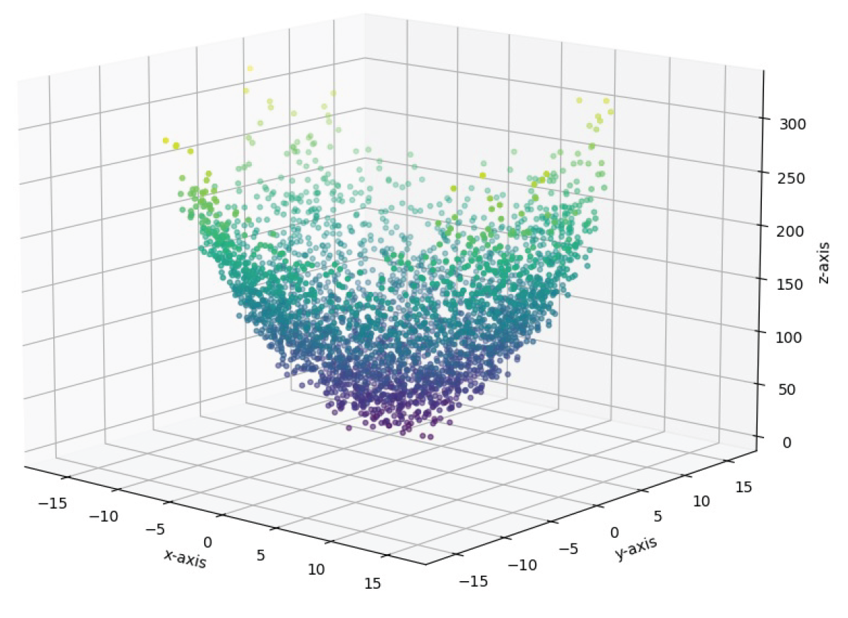
According to the diagram, the dispersion of the target function in the interval is greater than at other points. To find a more suitable solution, we re-evaluate the initial constant value using values smaller than the original, such as (see Figure 2) and (see Figure 3), and analyze the resulting graphs.
Based on the obtained graphs and the analysis of the dispersion of the objective function values, the best estimate for the dependent constant is .
Therefore, according to the acceptable approximation, the function:
is the most suitable option among the evaluated values for solving the PDE equation in this example.
3.2. Analysis and Investigation of the Dispersion of Prime Numbers
Finding prime numbers is one of the most fascinating topics in mathematics [12]. In this section, we employ the RDSF algorithm to study the distribution of prime numbers. Since any non-prime natural number can be expressed as a product of the numbers 1 through 9, we construct the n-dimensional spaces (M) required by the RDSF algorithm. These spaces consist of n-dimensional points that include the values 1 to 9. The largest number in this space is represented in the form:
For each number generated by multiplying the members of the n-dimensional space (), we define the value of the objective function at that point in the M-space as the number of times we add one to the resulting number to reach the first prime number. We then construct the n-dimensional space required by the RDSF algorithm and plot the final 3-dimensional diagrams for the 3-, 4-, and 5-dimensional spaces as examples.
In the two-dimensional space (see Figure 4), for the parameter of the first number after each product of the members of the space, the values 1, 2, 3, 4, and 5 are obtained with scattering counts of 14, 9, 5, 4, and 4, respectively. The highest concentration occurs at points with distances of 1 and 2, and the dispersion decreases for higher values.
In the three-dimensional space (see Figure 5), for the parameter of the first number after each product of the members of the space, the values 1, 2, 3, 4, 5, 6, 7, 8, 9, 11, and 13 are obtained, with scattering counts of 37, 18, 11, 9, 13, 1, 5, 1, 2, 2, and 1, respectively. The highest concentration occurs at points with distances of 1 to 5, and the dispersion decreases for higher values.
In the four-dimensional space (see Figure 6), for the parameter of the first number after each product of the members of the space, the values 1, 2, 3, 4, 5, 6, 7, 8, 9, 10, 11, 13, 14, 16, 17, 19, and 20 are obtained, with scattering counts of 75, 28, 21, 16, 26, 3, 19, 2, 7, 1, 9, 8, 1, 2, 5, 1, and 1, respectively. The highest concentration occurs at points with distances of 1 to 7, and the dispersion decreases for higher values. Additionally, points with a distance of 10, which were not observed in the three-dimensional space, appear in this space.
In the five-dimensional space (see Figure 7), for the parameter of the first number after each product of the members of the space, the values 1, 2, 3, 4, 5, 6, 7, 8, 9, 10, 11, 12, 13, 14, 15, 16, 17, 19, 20, 21, 23, 25, 26, 27, and 31 are obtained, with scattering counts of 127, 39, 39, 25, 50, 5, 38, 9, 15, 1, 31, 1, 20, 3, 1, 5, 13, 6, 1, 1, 4, 1, 1, 2, and 3, respectively. The highest concentration occurs at points with distances of 1 to 13, and the dispersion decreases for higher values. Additionally, points with distances of 12 and 15, which were not observed in the four-dimensional space, appear in this space.
In this application of the RDSF algorithm, by analyzing the results, the following conclusion can be drawn:
Corollary 2.
If represent an arbitrary m-dimensional space, then based on the degree of dispersion, the probability that the natural number:
is a prime number is higher for values of t between 1 and the dimension of the space (m), and lower for values greater than m.
3.3. Analysis and Investigation of the Behavior of Multivariate Arbitrary Real-Valued Functions
Assuming is a real-valued function of an arbitrary variable, we can use the RDSF algorithm to analyze the behavior of this function around a specific value. Using Python software, we select random values for the variables within their domain to form the M-space. Notably, the more points we generate, the more accurate the analysis becomes with the help of the RDSF algorithm.
Following the algorithm’s steps, we calculate the function for the set of randomly generated points. In the next step, we apply the MDS method to map these points into a 2-dimensional space while preserving their pairwise distances. Then, we add the value of the function at each n-dimensional point to create a 3-dimensional space. By plotting the 3-dimensional graph and observing the proximity of the dimension related to the function’s value, we can analyze the behavior of the function near the desired point.
Example 3.
The Rastrigin function is one of the most well-known test functions in the field of multivariate optimization and evolutionary algorithms. Finding the minimum of this function is a relatively challenging task due to its extensive search space and the large number of local minima [13].
where:
- is the input vector of dimension n.
- A is a constant, typically set to 10.
- n is the number of dimensions.
In the two-variable case (see Figure 8), the behavior of this function can be examined and visualized in a three-dimensional space, where the large number of local minima within a limited range is clearly observable.
In the three-variable case, since it is not possible to plot a four-dimensional space, one variable is typically held constant, and the remaining two variables along with the function value are analyzed in a three-dimensional space. By employing the RDSF algorithm and reducing the dimensions of the four-dimensional space, the behavior of the function can be intuitively examined in a three-dimensional space without assuming any variable to be constant, based on the behavior of all variables.
First, in the smaller range , using a computer and following the steps of the RDSF algorithm, random data is generated within this range, and the corresponding graph is obtained (see Figure 9). As can be observed, similar to the two-variable case, there are numerous local minima within this small range.
Next, in the larger range , using the RDSF algorithm and a computer, data is generated, and the observable space is obtained (see Figure 10). In this case, the global minimum of the function at the origin (zero point) is clearly visible, similar to the two-dimensional case.
In this problem, without imposing any constraints on the variables, the behavior of the function is visually examined, and previous findings regarding the existence of numerous local minima and a single global minimum at the origin are clearly confirmed.
References
- Wilke, C. O. (2019). Fundamentals of Data Visualization: A Primer on Making Informative and Compelling Figures. O’Reilly Media.
- Ma, Y. and Fu, Y. (2011). Manifold Learning Theory and Applications. CRC Press.
- van der Maaten, L., Postma, E., and van den Herik, J. (2009). Dimensionality Reduction: A Comparative Review. Journal of Machine Learning Research, 10:66–71.
- Murphy, K. P. (2022). Probabilistic Machine Learning: An Introduction. MIT Press.
- Hastie, T., Tibshirani, R., and Friedman, J. (2017). The Elements of Statistical Learning. 2nd edition. Springer.
- Goodfellow, I., Bengio, Y., and Courville, A. (2016). Deep Learning. MIT Press.
- LeVeque, R. J. (2007). Finite Difference Methods for Ordinary and Partial Differential Equations. SIAM.
- Tao, T. (2015). The Erdős Discrepancy Problem. Discrete Analysis, 1:1–29.
- McInnes, L., Healy, J., and Melville, J. (2018). UMAP: Uniform Manifold Approximation and Projection. Journal of Open Source Software, 3(29):861.
- Wang, L. & Zhang, H. (2023). Modern Multidimensional Scaling: Theory and Recent Advances. Journal of Machine Learning Research, 24(120), 1-45.
- Evans, L. C. (2010). Partial Differential Equations (2nd ed.). American Mathematical Society.
- Lemke Oliver, R. J. and Soundararajan, K. (2016). Unexpected biases in the distribution of consecutive primes. Proceedings of the National Academy of Sciences, 113(31), E4446–E4454.
- Chen, Z., & Gupta, A. (2023). Multiobjective Rastrigin function: Landscape analysis and algorithm benchmarking. IEEE Transactions on Evolutionary Computation, 27(4), 789-803.
Figure 1.
Scatter plot of the objective function for the constant value .
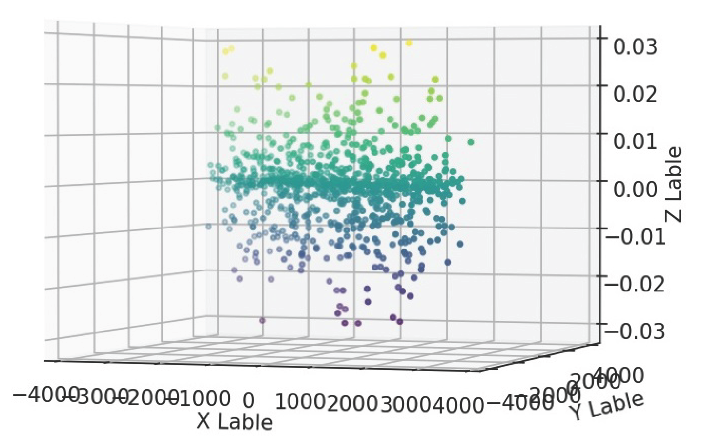
Figure 2.
Scatter plot of the objective function for the constant value .
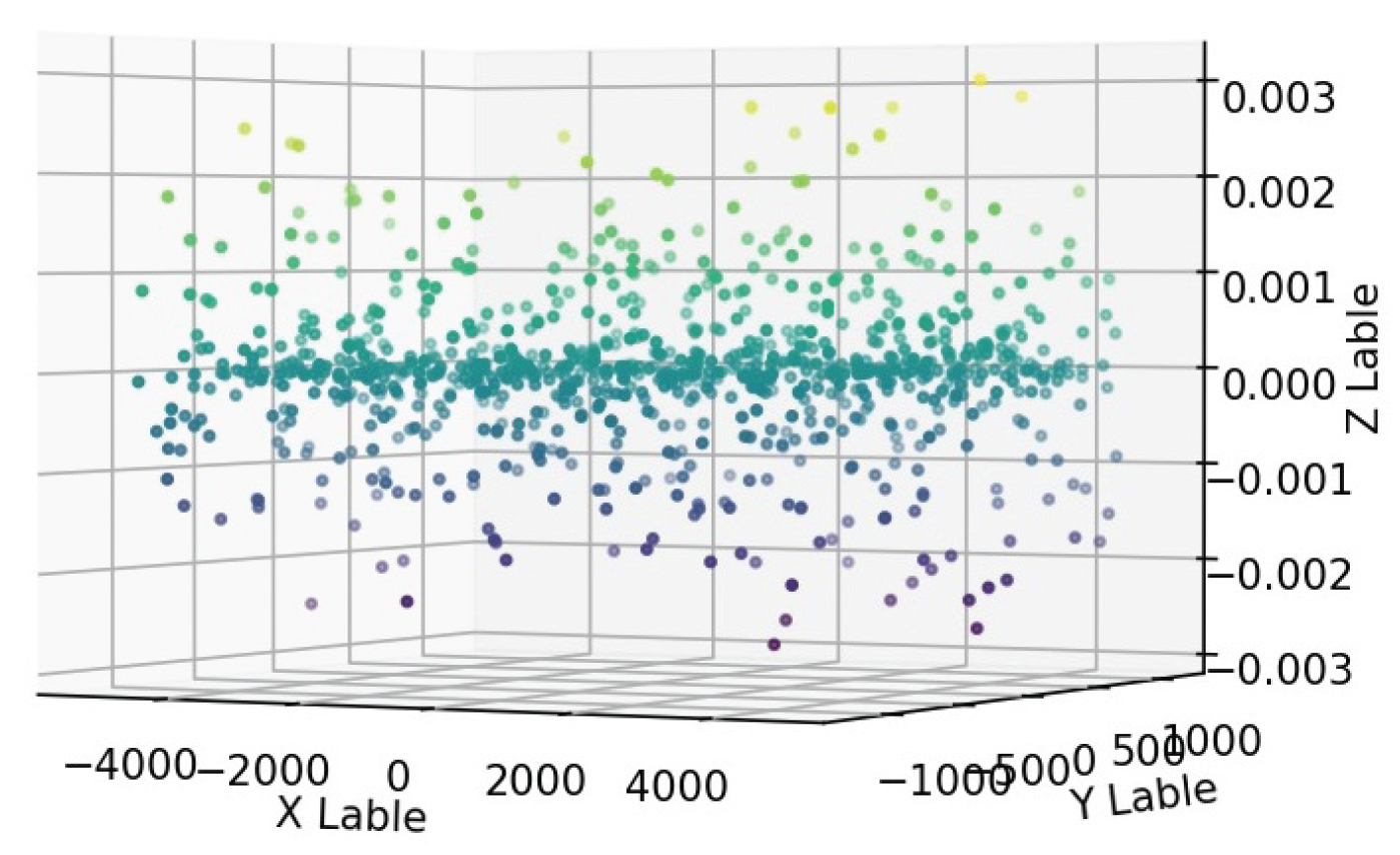
Figure 3.
Scatter plot of the objective function for the constant value .
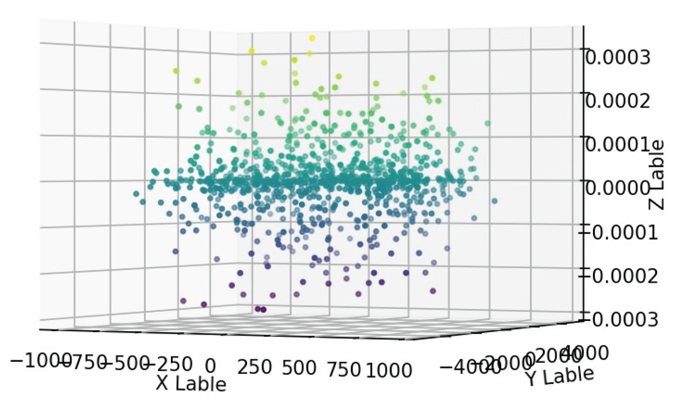
Figure 4.
Distance diagram to the first prime number in 2D space.
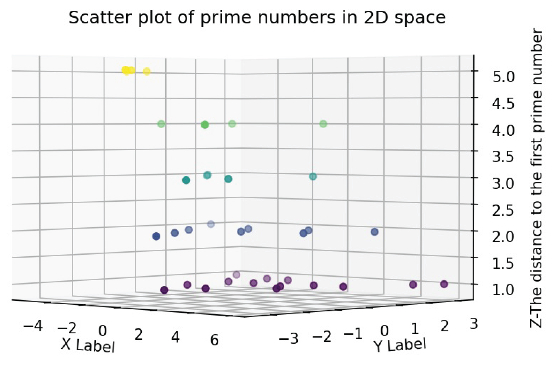
Figure 5.
Distance diagram to the first prime number in 3D space.
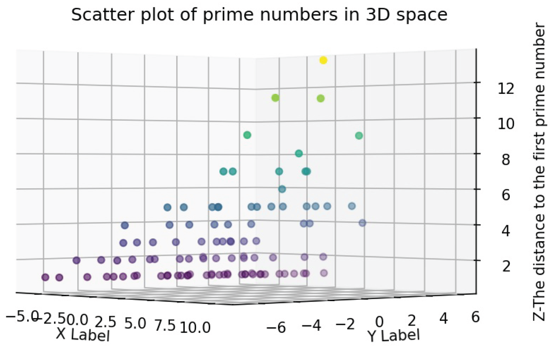
Figure 6.
Distance diagram to the first prime number in 4D space.
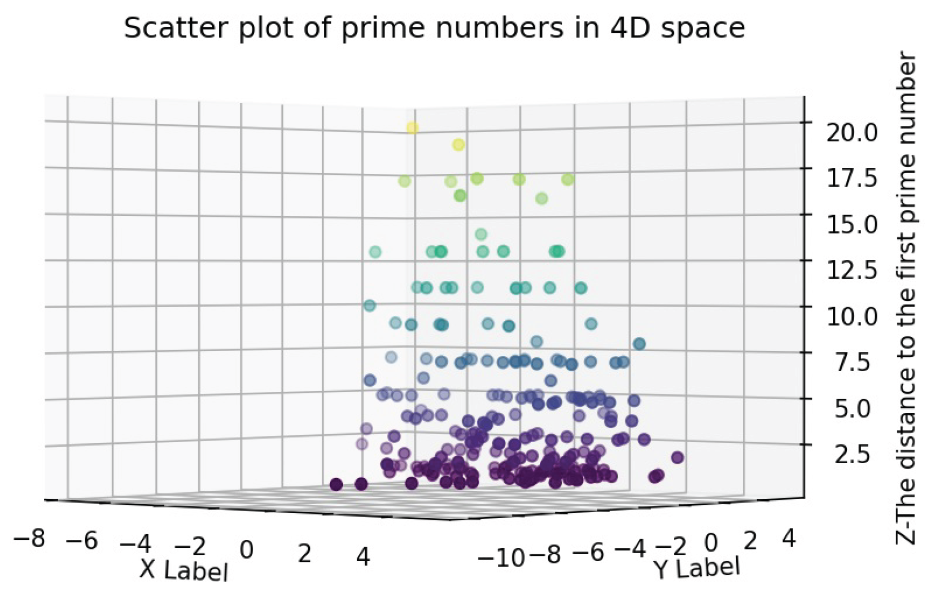
Figure 7.
Distance diagram to the first prime number in 5D space.
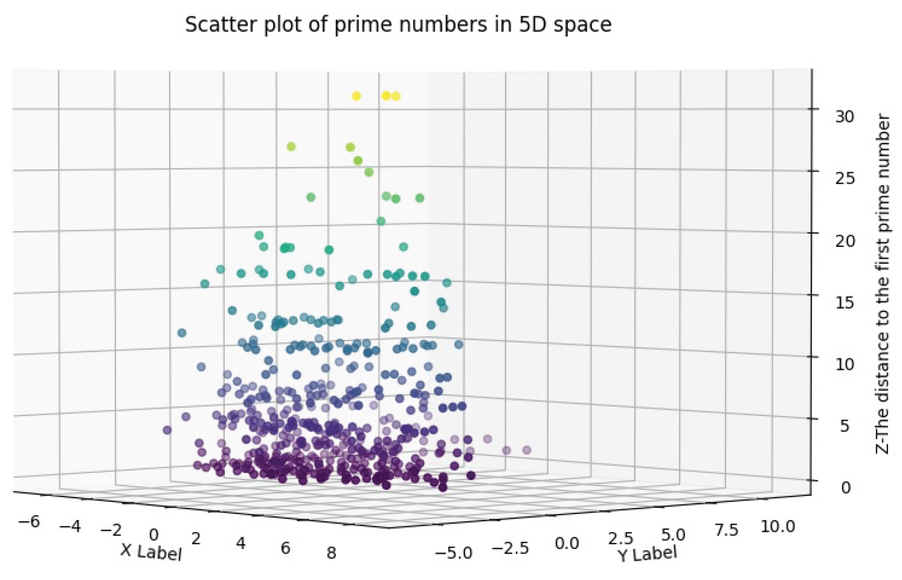
Figure 8.
Rastrigin Function (2 Variables)
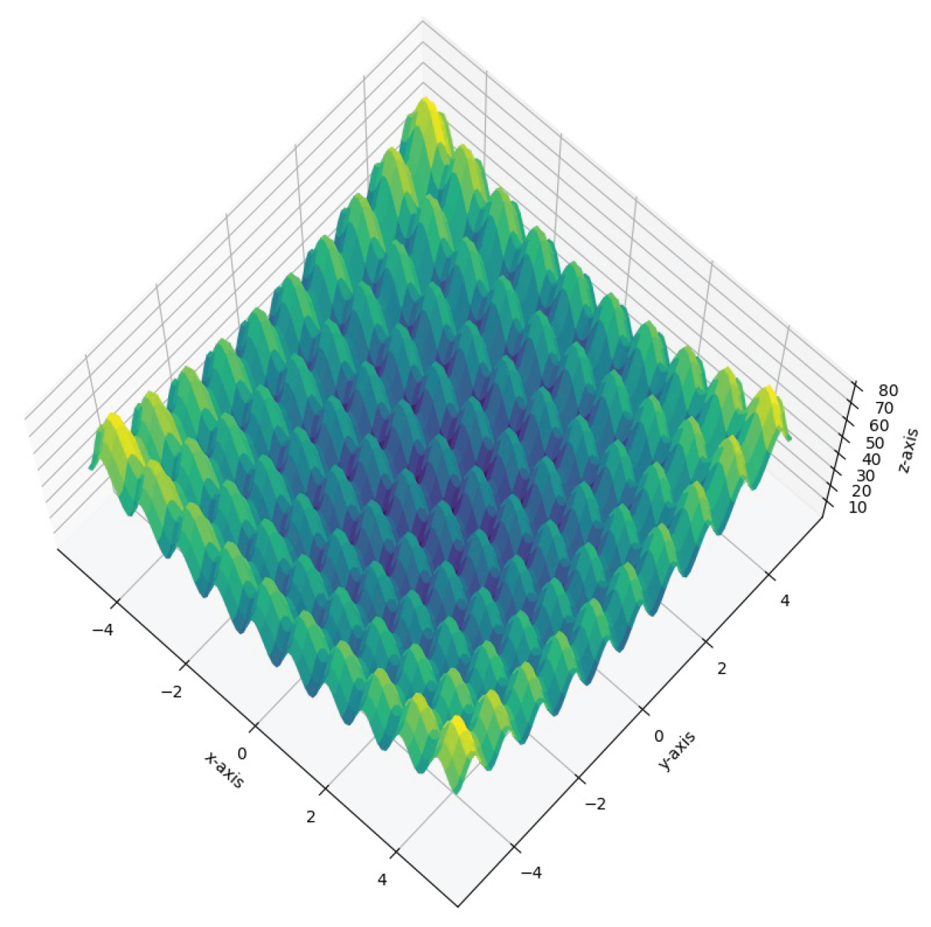
Figure 9.
Rastrigin Function (3 Variables) in the range
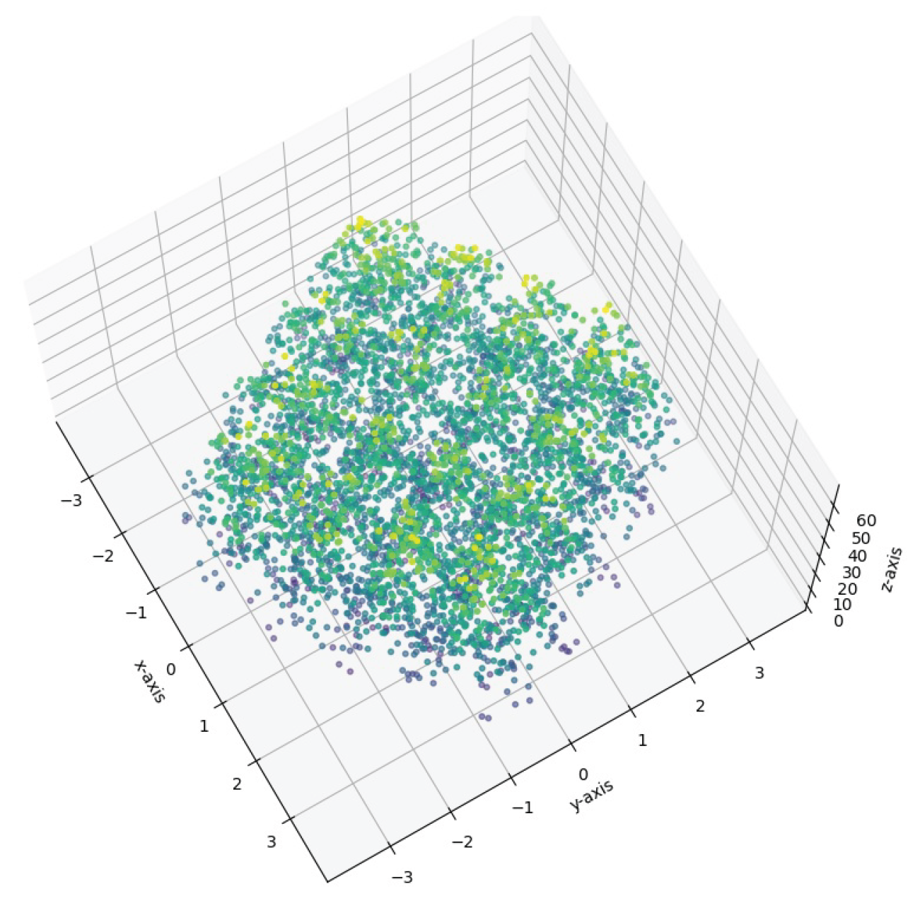
Figure 10.
Rastrigin Function (3 Variables) in the range
Disclaimer/Publisher’s Note: The statements, opinions and data contained in all publications are solely those of the individual author(s) and contributor(s) and not of MDPI and/or the editor(s). MDPI and/or the editor(s) disclaim responsibility for any injury to people or property resulting from any ideas, methods, instructions or products referred to in the content. |
© 2025 by the authors. Licensee MDPI, Basel, Switzerland. This article is an open access article distributed under the terms and conditions of the Creative Commons Attribution (CC BY) license (http://creativecommons.org/licenses/by/4.0/).
Copyright: This open access article is published under a Creative Commons CC BY 4.0 license, which permit the free download, distribution, and reuse, provided that the author and preprint are cited in any reuse.


