Modelling the Wealth and Probability of Default of Unsecured Loans: The Stochastic Partial Differential Equation Approach

1. Introduction

The financial industry is often grappling with the challenges posed by unsecured loans, which, unlike secured loans, are not designed to include collateral surety that might mitigate potential losses. In some cases, the information under which the loan is provided might be too scanty to provide a clear risk exposure. This category of loans, including personal loans, credit card debts and mobile (digital) loans, is particularly sensitive to fluctuations in economic conditions and borrower-specific factors. Effective risk management of such loans is crucial for financial stability and profitability of the lending institutions, thus making the development of robust analytical models to predict their loan performance a vital endeavor.

Recent economic downturns and evolving market dynamics have highlighted the shortcomings of traditional models in capturing the complex dependencies and the stochastic nature of unsecured loans(NBER, 2023). The need for more sophisticated modeling frameworks that can accommodate non-linear dynamics of these loans became clear. Such frameworks need to consider not only the inherent risk factors associated with the borrower and the loan but also the broader economic environment that significantly impacts loan portfolio performance (CEPR, 2023).

Stochastic Partial Differential Equations (SPDEs) offer a robust mathematical framework that capture systems influenced by random fluctuations and spatial variables. In finance, SPDEs have been effectively used to model a variety of complex phenomena including interest rates, pricing securities, and market volatility, demonstrating their versatility and application use cases (Wang et.al, 2023). Despite these successes, the application of SPDEs to analyze the wealth dynamics on unsecured loans has not been fully explored. This gap presents a unique opportunity to extend the utility of SPDEs to a new area within financial modeling. This paper aims to leverage on SPDEs to address this untapped area by introducing a novel approach that integrates both the random shocks and the spatial-temporal dimensions of unsecured loan wealth behavior, drawing on numerical methods such as those discussed by (Benth and Koekebakker, 2023) and extending them to include a Gaussian decay Kernel to enhance the model's practical application and efficacy.

The main goal of this research is to develop and validate a stochastic partial differential equation (SPDE) model to describe the wealth dynamics of unsecured loans. By incorporating macro-economic conditions, borrower characteristics, and loan-specific features, the model aims to serve as a comprehensive tool for predicting loan performance. This includes simulating different economic scenarios and assessing their impact on loan portfolios.

First, the study introduces an SPDE model driven by three correlated sources of random shocks that influence loan dynamics, which provides a more realistic representation of economic shocks and their propagation over time.

Second, the research presents methodological advancements in applying SPDEs to unsecured loans, focusing on the use of a Gaussian Kernel. This innovation allows for modeling the proportional effects of historical economic variability on loan wealth.

Third, the paper investigates both analytical and numerical solutions to the SPDE under Dirichlet’s boundary conditions, demonstrating the model's robustness and applicability to real-world scenarios.

Finally, the practical implications of the model for portfolio risk assessment are discussed.

Following the introduction, the paper is organized as follows: Section 2 focuses on the theoretical development of correlated Brownian motions, explaining how economic and borrower-specific factors are incorporated into both the diffusion and noise components. Section 3 deploys the correlated Brownian motions to the formulation of the SPDE model in unsecured loans. This section also highlights, the methodology for obtaining an analytical solution to the SPDE. Section 4 forms the basis for conducting numerical simulations for SPDE solution, offering insights into the model's behavior across various economic scenarios. Section 5 highlights the discussion, examining the practical implications of these findings, providing recommendations for financial practice and regulatory policy. We conclude the paper by summarizing the key contributions of the research and suggesting potential direction for future studies.

The study of unsecured loan dynamics opens a critical niche in financial modeling, intertwining elements of risk management, economic theory and stochastic processes. Recent advances have increasingly leveraged on advanced mathematical models such as Stochastic Partial Differential Equations (SPDEs) to capture the intricate behaviors of financial instruments under uncertainty. This section reviews the prevailing literature, highlighting seminal works and recent research advancements that inform our SPDE-based approach to modeling unsecured loans.

Historically, loan performance models have primarily focused on deterministic factors which employ statistical and econometric methods to predict default probabilities and losses. Classical models like the logistic regression-based credit scoring model (Hand and Henley, 1997) and Altman's Z-score model for credit risk (Altman, 1968) are examples of foundational works in the subject matter but often lack the capacity to incorporate stochasticity of the elements effectively.

The introduction of stochastic processes in finance by (Black and Scholes, 1973) through their groundbreaking work on option pricing (Black and Scholes, 1973) made a significant evolution. Duffie and Singleton (1999) extended these ideas to the credit market, through stochastic intensity model frameworks for modeling credit risk. However, these approaches predominantly focused on securities with explicit parameters and market pricing mechanisms.

The application of SPDEs in finance has traditionally been limited to derivatives pricing and interest rate modeling, as detailed by (Piterbarg, 2006) and (Filipović, 2009). More recently, researchers have begun to explore SPDEs in broader financial contexts, such as market liquidity and asset price volatility (Fouque and Langsam, 2013). These studies demonstrate the potential of SPDEs to model complex, multi-factorial dynamics in financial systems.

The concept of colored noise, representing temporally or spatially correlated stochastic processes, has been increasingly applied in economic modeling. The work by (Swishchuk, 2017) illustrates the use of Gaussian-colored noise to model market memory and price evolution, providing a theoretical basis for incorporating similar concepts into loan performance modeling. Applications in other areas such as reinforcement learning in artificial intelligence have also been explored (Onno, 2023).

The use of Gaussian kernels to smooth stochastic processes in time series analysis has been discussed by (Fan and Yao, 2003), who highlight their utility in handling non-stationary data. This approach is applicable to loan modeling, where economic conditions and borrower behaviors exhibit significant temporal variability and memory effects.

A significant gap in the literature is the application of Stochastic Partial Differential Equations (SPDEs) to model the wealth dynamics in unsecured loans, which face unique challenges due to the lack of collateral and the direct impact of economic conditions on borrower solvency. Existing research primarily focuses on securitized loans like mortgage-backed securities (MBS), where models like those developed by (Ahmad et.al, 2018) in their study of MBS pools effectively capture the dynamics of default and prepayment using SPDEs. Their work emphasizes the capability of SPDEs to handle complex, multi-layered risk factors in pooled mortgage loans, offering a comprehensive approach to understanding risk distributions over time and across different economic conditions​.

Our research extends these methodologies to unsecured loans by adapting the SPDE framework to account for the more idiosyncratic and less predictable nature of these loans. Unlike secured loans, where collateral offers a buffer against borrower risk of default, unsecured loans are more directly exposed to fluctuations in borrower financial health and broader economic shifts. By integrating factors such as market conditions, loan-specific characteristics, and individual borrower risk profiles into the SPDE model, we aim to provide a robust model of loan performance exhibiting formidable predictive power on risk of default.

This adaptation is inspired by the flexible and dynamic structural models proposed by (Cont and Minca, 2013), who used SPDEs to explore systemic risks in banking networks, suggesting a pathway for similar applications in loan modeling. Their approach to modeling interconnected risk factors in a network setting provides a valuable foundation for our model, which considers the interconnectedness of economic factors and individual borrower circumstances in unsecured lending. By building on the mathematical framework established by (Ahmad et al., 2018) and adapting it to the unique characteristics of unsecured loans, we address a critical research gap. This approach not only enhances our understanding of loan dynamics under varying economic conditions but also makes a significant contribution to financial risk management, particularly in the assessment and management of unsecured loan portfolios.

The literature underscores a growing recognition of the need for advanced mathematical models in financial analysis. The shift towards using SPDEs in loan modeling represents a significant leap into more robust and relatively accurate approaches to predictive and realistic risk management solutions in the finance industry. The adaptation of SPDE frameworks to unsecured loan dynamics, as suggested by the referenced studies, offers a promising avenue for future research and practical application in financial risk assessment.

2. The Model Setup

This section we develop the Stochastic Partial Differential Equation (SPDE) model to capture the dynamics of wealth process in unsecured loans. We will first formulate the wealth process of an unsecured loan with factors drawn from the market, loan and individual attributes, before embarking on its application to the SPDE.

2.1. Correlated Brownian Motion

For an unsecured loan, the wealth process $X_i\left(t\right)$ should reflect the borrower, $i^{\text{'}}s,$ability to repay the loan, considering various sources of financial pressures and economic conditions. The SDE for $X_i\left(t\right)$ can be modeled as follows:

$${dX}_i\left(t\right)={\mu }_i\left(t, X_i\left(t\right)\right)dt+{\sigma }_M{dW}_t^M+{\sigma }_L{dW}_t^L+{\sigma }_i{dW}_t^i$$

(1)

Where:

${\mu }_i\left(t, X_i\left(t\right)\right)$ denotes the drift function of the wealth process, representing the average change of the wealth of individual $i$ over a given period of time t.

${\sigma }_M, {\sigma }_L and {\sigma }_i$ are the volatilities related to the market, the loan portfolio and the idiosyncratic factors of the $i^{th}$ borrower respectively.

$W_t^M, W_t^L and W_t^i$ are the respective dependent Brownian motions for the market, the loan portfolio and the idiosyncratic risk sources.

In order to incorporate the dependency amongst the three Brownian motions, we need to formulate the correlation matrix:

$$\sum =\left[\begin{array}{ccc}1& {\rho }_{iL}& {\rho }_{iM}\\ {\rho }_{iL}& 1& {\rho }_{LM}\\ {\rho }_{iM}& {\rho }_{LM}& 1\end{array}\right]$$

We will assume that the correlations above are constant under the Gaussian copula and are mathematically obtained using Cholesky decomposition of three correlated paths and can be expressed as linear combinations of independent Brownian motions $W_t^1$, $W_t^2$ and $W_t^3$ so that the dependent Brownian motions can be expressed as

$$W_t^i=W_t^1{W}_t^L={{\rho }_{iL}W}_t^1+{\sqrt{1-{\rho }_{iL}^2}W}_t^2{W}_t^M={{\rho }_{iM}W}_t^1+{{\rho }_{LM}({\rho }_{iL}{W}_t^1+\sqrt{1-{\rho }_{iL}^2}W}_t^2) +\sqrt{1-{\rho }_{iM}^2-{\rho }_{LM}^2-2{\rho }_{iL}{\rho }_{iM}{\rho }_{LM}}{W}_t^3$$

The individual factors can evolve independently and represented by the noise $W_t^1$, while specific loan conditions that are unique to the loan book are captured by $W_t^2$; while general market trends of economic growth are captured by $W_t^3$.

The Cholesky decomposition of the correlation matrix $\sum$can be factored into a product of the lower triangular matrix $L$ and its transpose $L^T$ such that:

$$\sum =L{L}^T$$

Where $L$ is the Cholesky factor matrix with the structure

$$L=\left(\begin{array}{ccc}1& 0& 0\\ {\rho }_{iL}& \sqrt{1-{\rho }_{iL}^2}& 0\\ {\rho }_{iM}& {\displaystyle \frac{{\rho }_{LM}-{\rho }_{iL}{\rho }_{iM}}{\sqrt{1-{\rho }_{iL}^2}}}& \sqrt{1-{\rho }_{iM}^2-{\rho }_{LM}^2-2{\rho }_{iL}{\rho }_{iM}{\rho }_{LM}}\end{array}\right)$$

This matrix shows the individual wealth responses to sources of shocks influenced by personal characteristics, loan conditions and the broader economic changes.

We aim to create a single sourced Brownian motion that will encapsulate all the correlated Brownian motions. A plausible formulation would be to use a time dependent vector quantity in the planes of orthogonal representation of the three sources of variations. Suppose ${\widehat{W}}_i\left(t\right)$ is the vector representation the overall Brownian motion effect on $X_i\left(t\right)$, we can express ${\widehat{W}}_i\left(t\right)$ combining the total effect of the Market, the Loan and the idiosyncratic factors as a linear combination of the independent Brownian motions as:

$${\widehat{W}}_i\left(t\right)=L\left(\begin{array}{c}{W}_t^1\\ W_t^2\\ W_t^3\end{array}\right)$$

(2)

Thus, the protracted SDE modelling the dynamics of $X_i\left(t\right)$ with the correlated Brownian motions bounded by Lipschitz conditions becomes

$${dX}_i\left(t\right)={\mu }_i\left(t,X_i\left(t\right)\right)dt+\sigma (t,X_i\left(t\right))d{\widehat{W}}_i\left(t\right)$$

(3)

Where,

${\mu }_i\left(t, X_i\left(t\right)\right)$, the drift term represents the deterministic part of the wealth dynamic drawn from all sources of risks.

$\sigma (t, X_i\left(t\right))$, the diffusion term modulating the sensitivity of $X_i\left(t\right)$ under the risk factors of ${\widehat{W}}_i\left(t\right).$The Weiner Process, ${\widehat{W}}_i\left(t\right)$, can be standardized to aggregate all the three sources of variation through a discretization criterion for data analysis.

2.2. Portfolio Dynamics

In order to develop the loss model, we need to formulate risks from their root causes. Every loan in a portfolio bears risk of default, prepayments risk and refinancing risk. The occurrence of any of the above three events will lead to unrealized losses in the loan portfolio. Therefore, it is in the interest of the lender to model the wealth of the borrower in anticipation of any of the three risks. The wealth process first requires a logistic transformation mapping into a density function. Let $Y_i\left(t\right)$as the corresponding density function mapping the wealth process $X_i\left(t\right)$ to a bounded interval (0,1).

Using Ito’s Lemma, the dynamics associated with the transformed process $Y_i\left(t\right)$ can be shown as

$$d{Y}_i\left(t\right)={\mu }_i\left(t, Y_i\left(t\right)\right)dt+{\sigma }_i\left(t, Y_i\left(t\right)\right)d{\widehat{W}}_i\left(t\right)$$

(4)

Unsecured loans can be clustered into pools and exit causes characterized by maturity of the loan to term, early repayment (prepayment), default and refinancing; with these events being mutually exclusive and independent in relation to the dynamics of the loan pool.

While modeling each of the exit times independently is likely to provide useful insights to each of these exit risks, we will confine our study to the probability of default as a risk measure.

For our model involving the stochastic density function $Y_i\left(t\right)$, we can establish a technical condition as a sensitivity measure of the volatility or stability of the risk probability over time interval $[s,t]$, such that

$$\mathbb{E}{(Y_i\left(t\right)-Y_i(s\left)\right)}^2={\int }_s^t\mathbb{E}\left[{{\sigma }_i\left(u, X_i\left(u\right)\right)}^2{Y_i}^2\left(u\right){\left(1-Y_i\left(u\right)\right)}^2\right)]du$$

(5)

2.3. Aggregate Loss and the Empirical Process

Consider the aggregate loss, $L^n\left(t\right),$ defined as the count of losses over the individual processes $Y_i\left(t\right)$ at time $t$, representing the defaults and empirical process $u^n\left(t\right)$, defined as the average of some measurable function $f$ applied to the processes $Y_i\left(t\right)$ where:

$$L^n\left(t\right)={\displaystyle \frac{1}{n}}\sum _{i=1}^n{1}_{\{{\tau }_i\le t\}}$$

$$u^n\left(t\right)={\displaystyle \frac{1}{n}}{\sum }_{i=1}^n{1}_{\{{\tau }_i\le t\}}{\delta }_{Y_i\left(t\right)}$$

(6)

The process $u^n\left(t\right)$ can be interpreted as the distribution of the loan values among borrowers with outstanding loans in the portfolio by time $t$. The Dirac delta ${\delta }_{Y_i\left(t\right)}$ highlights the value as $Y_i\left(t\right)$.

The total filtration ${\mathcal{F}}_t$ represents the filtration up to time $t$, which includes all relevant information from both the market and the loan portfolio affecting the individual loan and is represented as:

$${\mathcal{F}}_t={\mathcal{F}}_t^M\bigvee {\mathcal{F}}_t^L$$

(7)

where ${\mathcal{F}}_t^M$ is the filtration generated by the market factors and ${\mathcal{F}}_{\mathit{t}}^{\mathit{L}}$ is the filtration generated by the loan-specific factors.

There exists a relationship between $u^n\left(t\right)$ and $L^n\left(t\right)$ shown in (Ahmad et al. 2018), Theorem 2.3 such that

$$1-u^n\left(t\right)\left(\mathrm{0,1}\right)=L^n\left(t\right)$$

(8)

Where $u^n\left(t\right)\left(\mathrm{0,1}\right)$ measures the total surviving loan proportion, incorporating considerations of both the market trends and the individual loan behaviors up to time t.

Theorem 1. [Birkhoff’s Ergodic Theorem]: Birkhoff’s Ergodic Theorem states that for a measure preserving transformation $T$ on a probability space $(\mathsf{\Omega },\mathcal{F},\mathbb{P})$ and with an integrable function $f$, the time averages of $f$ converges almost surely in $L^1$ to the space average of $f:$

$${\displaystyle \frac{1}{n}}\sum _{i=0}^{n-1}f\left(T^i\varpi \right)\begin{array}{c}a.s\\ ⟶\\ \mathrm{n}\to \mathrm{\infty }\end{array}E\left(f\right) \mathrm{for} \mathrm{almost} \mathrm{all} \varpi$$

The processes $Y_i\left(t\right)$ are assumed to be identically distributed and ergodic for all $i$. Using Birkhoff’s Ergodic Theorem, the aggregate loss function $L^n\left(t\right)$ and the empirical process, $u^n\left(t\right)$ converges to $L\left(t\right) and u\left(t\right)$ respectively, such that

$${\sum }_{\mathrm{n}\to \mathrm{\infty }}{L}^n\left(t\right)=P\left({\tau }_i\le t|{\mathcal{F}}_t\right)=1-u^n\left(t\right)\left(\mathrm{0,1}\right)\text{ and}$$

$${\sum }_{\mathrm{n}\to \mathrm{\infty }}{u}^n\left(t\right)=P\left(Y_i\left(t\right)\in S;{\tau }_i\le t|{\mathcal{F}}_t\right) \mathrm{for} S\in \left(\mathrm{0,1}\right)$$

As $\mathrm{n}\to \mathrm{\infty }$, and assuming that each $Y_i\left(t\right)$ are $i.i.d$ergodic processes and the loan’s first exit times $\tau$are independent of the $Y_i\left(t\right)$ paths,

$${\sum }_{\mathrm{n}\to \mathrm{\infty }}{u}^n\left(t\right)=E\left(1_{\left\{\tau <t\right\}}{\delta }_{Y\left(t\right)}\right)$$

(9)

The limit process $E\left(1_{\left\{\tau <t\right\}}{\delta }_{Y\left(t\right)}\right)$ is a probabilistic measure on the state space of the loan that quantifies the distribution on active loans in the portfolio at any time $t$ as the number of loans become very large.

Let $M$ denote the space of finite measures on [0,1] equipped with the Skorokhod $J1$topology of weak convergence. Then the sequence of the empirical processes $u^n\left(t\right)\text{'}s$, defined as a measure-valued cadlag processes which as $\mathrm{n}⟶\mathrm{\infty },$ converges in law to $u\left(t\right)$. Consequently, the sequence of loss processes, $L^n$ also converges in law to $L$, where $L$ is the limit loss process in the cadlag real valued paths.

Assuming $Y_i\left(t\right)$ for $i=\mathrm{1,2},\dots ,n$ and that equation 9 holds for large $n$, we aim to derive the limit SPDE.

We define the empirical density $u(x,t)$ as a measure representing the density of states $Y_i\left(t\right)$ at position $x$ and time $t$ so that:

$$u\left(x,t\right)={\displaystyle \frac{1}{n}}\sum _{i=1}^n\delta (x-Y_i(t\left)\right)$$

(10)

where $\delta$ is the Dirac delta function, placing mass at the locations of each $Y_i\left(t\right).$The function $u(x,t)$ must be adapted to the filtration on equation 7, generated by the collective noise process ${\widehat{W}}_i\left(t\right).$

2.4. Tightness and Convergence of the Empirical Measure

Theorem 2. [Theorem of Tightness]: Definition: A family of probability measures ${\mathcal{P}}_n$ on a metric space $\mathcal{M}$ is said to be tight for every $ϵ>0$, there exists a compact set $K_{ϵ}\subset \mathcal{M}$ satisfying the condition that:

$$\mathbb{P}\left({\mathcal{P}}_n\in K_{ϵ}\right)>1-ϵ \forall n{\in \mathbb{z}}^{+}$$

(11)

We seek to verify the uniform boundedness and equicontinuity of the empirical measure, $u^n\left(t\right).$Thereby, establishing the tightness over a suitable space function $\mathcal{S}\left(\left[\mathrm{0,1}\right],\mathcal{G}\left[\mathrm{0,1}\right]\right)$drawn over a space of finite measure $\mathcal{G}\left[\mathrm{0,1}\right]$ in the interval $\left[\mathrm{0,1}\right]$.

Uniform boundedness in probability holds if the total mass is constrained within the limit interval. This holds for $u^n\left(t\right)$ since for $ϵ>0$, there exists $K_{ϵ}$ such that

$$\mathbb{P}\left({\int }_0^T{\int }_0^1\left|u^n\left(x,t\right)\right|dxdt>K_{ϵ}\right)<ϵ \forall n{\in \mathbb{z}}^{+}$$

as long as $u^n\left(t\right)$ is a probability measure with the condition

$${\int }_0^1{u}^n\left(x,t\right)dx=1 \forall \mathrm{f}\mathrm{o}\mathrm{r}t\in \left[0,\mathrm{T}\right]$$

(12)

Moreover, we seek to establish the continuity of the empirical density measure $u^n\left(t\right).$ This can be achieved by ascertaining that it does not vary wildly over small changes in time. To demonstrate this, for every $ϵ>0$ and $K_{ϵ}>0$, there exists a $\delta >0$ such that whenever $\left|t-s\right|<\delta$, then,

$$\mathbb{P}\left({sup}_{x\left[\mathrm{0,1}\right]}|u^n\left(x,t\right)-u^n\left(x,s\right)|>K_{ϵ}\right)<ϵ \mathrm{uniformly} \mathrm{in} n \mathrm{f}\mathrm{o}\mathrm{r} 0\le s<t\le T.$$

Since both $Y_i\left(t\right)$ and the Dirac delta are continuous, then it follows that the empirical measure is also continuous on small differences $\left|u^n\left(x,t\right)-u^n\left(x,s\right)\right|,$ over small $\delta >0\square$

2.5. Weak Convergence of $u^n\left(x,t\right)$ to a Limit Measure $u(x,t)$

Theorem 3. [Prokhorov’s Theorem]: Prokhorov’s Theorem states that a sequence of tight probability measure defined on complete separable metric space, such as the Polish Space in the interval $\left[\mathrm{0,1}\right]$, is relatively compact. The implication of this is that each of these sequences converges weakly in the order of their progression.

Since $u^n\left(x,t\right)$ is tight, then ${\left\{u^n\left(x,t\right)\right\}}_n$ sequence is relatively compact over the space of probability measure equipped with topological weak convergence. Thus, it follows that for a subsequence ${\left\{u^{n_m}\left(x,t\right)\right\}}_{n_m}$ and a probability measure $u\left(x,t\right)$,

$${\left\{u^{n_m}\left(x,t\right)\right\}}_{n_m}\to u\left(x,t\right)\mathrm{whenever} m\to \infty$$

2.6. Limit Identity Using Skorokhod’s Representation Theorem

Theorem 4. [Skorokhod Theorem]: Skorokhod Theorem improves the weak convergence formulation of $u^n\left(x,t\right)$ to almost sure results by transforming it to, potentially, a different probability space, with desirable contextual properties such as uniqueness in law.

Lex ${\left\{U\right\}}_n$ be a sequence of random variables with usual probability space $(\mathsf{\Omega }.\mathcal{F},\mathbb{P})$ with weak distributional convergence to $U.$ There exists another set of random variables ${\left\{U^{*}\right\}}_n$ and $U^{*}$ equipped with probability space $({\mathsf{\Omega }}^{*},{\mathcal{F}}^{*},{\mathbb{P}}^{*})$ such that

(13)

To proof that Skorokhod Theorem holds for $u^n\left(x,t\right),$ first we need to construct the probability spaces.

Let $U^{*}(x,t)$ and $U(x,t)$ be the CDFs of the random measures $u\left(x,t\right)\mathrm{a}\mathrm{n}\mathrm{d}{u}^n\left(x,t\right)$ respectively. Since $u^n\left(x,t\right)⟶u(x,t)$ in distribution, then it follows that $U^{*}(x,t)$ converges to $U(x,t)$ at every point of its continuity. Subsequently, if the quantile functions of $U^{*}(x,t)$ and $U(x,t)$ are denote as $Q^{*}(x,t)$ and $Q(x,t)$ respectively, then

$$Q^{*}\left(x,s\right)=\mathrm{i}\mathrm{n}\mathrm{f}\{x\in \mathbb{R}:U^{*}(x,t)\ge s\} \text{and}$$

$$Q\left(x,s\right)=\mathrm{i}\mathrm{n}\mathrm{f}\{x\in \mathbb{R}:U(x,t)\ge s\} \text{for} s\in [0,1]$$

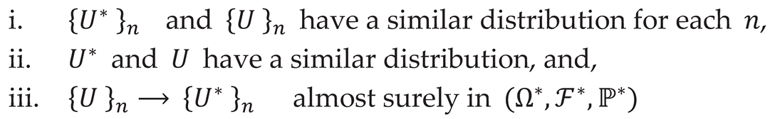
A uniformly distributed random variable, $Z$, is defined over the interval $\left[\mathrm{0,1}\right]$ on a new probability space $({\mathsf{\Omega }}^{*},{\mathcal{F}}^{*},{\mathbb{P}}^{*})$. Defining $u^{*n}\left(x,t\right) and u^{*}\left(x,t\right)$ as follows

$u^{*n}\left(x,t\right)=Q^{*}\left(x,z\right)$ and $u^{*}\left(x,t\right)=Q\left(x,z\right)$Therefore we deduce that the distributions of $u\left(x,t\right)\mathrm{a}\mathrm{n}\mathrm{d}{u}^n\left(x,t\right)$ are similar to the distributions of ${u^{*}\left(x,t\right) \mathrm{a}\mathrm{n}\mathrm{d}u}^{*n}\left(x,t\right)$since the quantile transformation maps the uniform distribution to those of $u\left(x,t\right)\mathrm{a}\mathrm{n}\mathrm{d}{u}^n\left(x,t\right)$. Since $Q^{*}(x,t)$ converges to $Q(x,t)$ at all points of continuity of $U(x,t)$ and $Z$ is almost surely continuous Ahmed et al (2018, Lemma 4.1), then $Q^{*}\left(x,z\right)⟶$ $Q\left(x,z\right)$ almost surely; thus $u^{*n}\left(x,t\right) ⟶ u^{*}\left(x,t\right)$ almost surely in $({\mathsf{\Omega }}^{*},{\mathcal{F}}^{*},{\mathbb{P}}^{*})$. □

3. SPDE for the Empirical Density Measure

The process $u(x,t)$ under the conditions of the formulation of equation 12 and with sufficient smoothness, converges similar to a function, $f$, as shown by Ahmed et. al. (2018), that satisfies an SPDE of the form

$${\displaystyle \frac{\partial f}{\partial t}}=\mu \left(x,t\right){\displaystyle \frac{\partial f}{\partial x}}+{\displaystyle \frac{1}{2}}{\sigma }^2\left(x,t\right){\displaystyle \frac{{\partial }^{2}f}{\partial x^2}}=Lf$$

(14)

The operator $L=\mu \left(x,t\right){\displaystyle \frac{\partial }{\partial x}}+{\displaystyle \frac{1}{2}}{\sigma }^2\left(x,t\right){\displaystyle \frac{{\partial }^2}{\partial x^2}}$ , is the generator of the stochastic process and $f$ is carefully chosen to meet some test function condition. Now we aim to show that our empirical density process $u(x,t)$ has a general SPDE formulation given as

$${\displaystyle \frac{\partial u}{\partial t}}=Lu+(noise term)$$

Specifically, $u(x,t)$ satisfies the SPDE form represented as follows:

$${\displaystyle \frac{\partial u(x,t)}{\partial t}}=-{\displaystyle \frac{\partial }{\partial x}}\left\{\mu \left(x,t\right)u\left(x,t\right)\right\}+{{\displaystyle \frac{1}{2}}{\displaystyle \frac{{\partial }^2}{\partial x^2}}\{\sigma }^2\left(x,t\right)u\left(x,t\right)\}+Correlated Noise$$

(15)

Consider the empirical density process $u(x,t)$ as defined in equation 13 and $f$to be a continuous and twice differentiable, $C^2$, function following the Dirichlet boundary conditions over the interval $\left[\mathrm{0,1}\right]$, we have that

$$f\left(0\right)=f\left(1\right)=0 \text{(Dirichlet boundary condition)}$$

Let the infinitesimal generator associated with the stochastic process $Y_i\left(t\right)$ be defined as equation 14 above. The behaviour of $u(x,t)$ under the given test function, $f,$ can be analyzed by passing limits inside integrals on conditions of uniform integrability and dominated convergence such that

$$f\left(x\right)={\int }_0^{1}u\left(x,t\right)f\left(x\right)dx={\displaystyle \frac{1}{n}}\sum _{i=1}^{n}f\left(Y_i\left(t\right)\right)$$

(16)

The temporal derivative of the above equation given $\mathcal{L}$ over $f$ is given as

$${\displaystyle \frac{\partial }{\partial t}}{\int }_0^{1}u\left(x,t\right)f\left(x\right)dx={\displaystyle \frac{1}{n}}\sum _{i=1}^{n}Lf\left(Y_i\left(t\right)\right)$$

$$={\displaystyle \frac{1}{n}}\sum _{i=1}^n\left(\mu \left(Y_i\left(t\right),t\right)f^{\text{'}}\right(Y_i\left(t\right))+{\displaystyle \frac{1}{2}}{\sigma }^2\left(Y_i\left(t\right),t\right)f^{\text{'}\text{'}}\left(Y_i\left(t\right)\right)$$

As $n⟶\infty$ and if $Y_i\left(t\right)$ are dense in [0,1], $u(x,t)$ becomes smooth such that

$${\int }_0^{1}u\left(x,t\right)Lf\left(x\right)dx={\int }_0^1\left(u\left(x,t\right)\right(\mu \left(x,t\right)f^{\text{'}}\left(x\right)+{\displaystyle \frac{1}{2}}{\sigma }^2\left(x,t\right)f^{\text{'}\text{'}}\left(x\right))dx ={\int }_0^{1}u\left(x,t\right)\left(\mu \left(x,t\right)f^{\text{'}}\left(x\right)\right)dx+{\int }_0^1{\displaystyle \frac{1}{2}}{u(x,t)\sigma }^2\left(x,t\right)f^{\text{'}\text{'}}\left(x\right)dx$$

Solving further through integration by parts for each of the two integrals separately, ${\int }_0^{1}u{v}^{\text{'}}dx=uv-{\int }_0^1{u}^{\text{'}}vdx$ ,

Starting with the first integral, let $u=u(x,t)$ and $v^{\text{'}}=\mu \left(x,t\right)f^{\text{'}}\left(x\right)$. We can see that $u(x,t)$ has no $x-derivative$ due to the integration properties of the Dirac delta functions. Therefore

$${\int }_0^{1}u\left(x,t\right)\left(\mu \left(x,t\right)f^{\text{'}}\left(x\right)\right)dx={\left[u\left(x,t\right)\left(\mu \left(x,t\right)f\left(x\right)\right)\right]}_0^1-{\int }_0^1{\displaystyle \frac{\partial }{\partial x}}u\left(x,t\right)\left(\mu \left(x,t\right)f\left(x\right)\right)dx=-{\int }_0^1{\displaystyle \frac{\partial }{\partial x}}u\left(x,t\right)\left(\mu \left(x,t\right)f\left(x\right)\right)dx$$

For the second integral we apply integration by parts twice such that , $u=u(x,t)$ and $v={\sigma }^2\left(x,t\right)f\left(x\right)$, then

$${\int }_0^{1}u{v}^{\text{'}\text{'}}dx=u{v}^{\text{'}}-{\int }_0^1{u}^{\text{'}}vdx=u{v}^{\text{'}}-(u^{\text{'}}v-{\int }_0^1{u}^{\text{'}\text{'}}vdx)$$

Therefore

$${\int }_0^1{\displaystyle \frac{1}{2}}{u(x,t)\sigma }^2\left(x,t\right)f^{\text{'}\text{'}}\left(x\right)dx={\displaystyle \frac{1}{2}}{\int }_0^1{\displaystyle \frac{{\partial }^2}{\partial x^2}}u(x,t){\sigma }^2\left(x,t\right)f\left(x\right)dx$$

since $u{v}^{\text{'}} and u^{\text{'}}v$ vanishes under the boundary integrals.

Combining the two results, from integration we see that our empirical density yields the SPDE in integral form

$${\int }_0^{1}u\left(x,t\right)Lf\left(x\right)dx=-{\int }_0^1{\displaystyle \frac{\partial }{\partial x}}u\left(x,t\right)\left(\mu \left(x,t\right)f\left(x\right)\right)dx+{\displaystyle \frac{1}{2}}{\int }_0^1{\displaystyle \frac{{\partial }^2}{\partial x^2}}u\left(x,t\right){\sigma }^2\left(x,t\right)f\left(x\right)dx$$

(17)

This equation describes how the macroscopic density $u\left(x,t\right)$ evolves over time, taking into account both the drift and diffusion effects from the underlying stochastic processes. By incorporating an externally correlated smoothened noise function, we obtain SPDE of the form shown in equation 15.

The Dirichlet boundary conditions are crucial in this derivation, ensuring that no flux of probability occurs at the boundaries, thus containing the dynamics within the specified domain [0,1]. □

3.1. Limit Characterization

In this section we establish the distributional behavior of $u\left(x,t\right)$ to the SPDE for any given test function $f$ using the Martingale problem approach.

Let $M_t^f$ be a martingale process adapted to the filtration ${\mathcal{F}}_t$ generated by $u(x,t)$ such that

$${E(M}_t^f\left|{\mathcal{F}}_s\right)=M_s^f \text{and} M_t^f=〈u\left(x,t\right),f〉-〈u\left(x,0\right),f〉-{\int }_0^t〈u\left(x,s\right),L_{s}f〉ds$$

Where $〈u\left(x,t\right),f〉$ is the integral of $f$ over the random measure $u(x,t)$ and

$$L_{s}f==-{\displaystyle \frac{\partial }{\partial x}}\left\{\mu \left(x,s\right)u\left(x,s\right)\right\}+{\displaystyle \frac{1}{2}}{\displaystyle \frac{{\partial }^2}{\partial x^2}}\left\{{\sigma }^2\left(x,s\right)u\left(x,s\right)\right\}$$

We need to show that $M_t^f$ is a martingale over $0\le s<t$.

$$M_t^f={\int }_0^{1}u\left(dx,t\right)f\left(x\right)ds-{\int }_0^{1}u\left(dx,0\right)f\left(x\right)ds-{\int }_0^1{\int }_0^t{L}_{s}f\left(x\right)u(dx,s)ds$$

From the Skorokhod’s weak convergence, we extend the concept to integrals for $t>0$ and $n⟶\infty$,

$${\int }_0^1{u}^n\left(dx,t\right)f\left(x\right)ds⟶{\int }_0^{1}u\left(dx,t\right)f\left(x\right)ds{\int }_0^1{\int }_0^t{L}_{s}f\left(x\right)u^n(dx,s)ds \text{and} ⟶{\int }_0^1{\int }_0^t{L}_{s}f\left(x\right)u(dx,s)ds$$

In order to prove the Martingale property, we consider the expected increments to satisfy:

$${E(M}_t^f-M_s^f\left|{\mathcal{F}}_s\right)=M_s^f=0=E\left(\right[〈u\left(x,t\right),f〉-〈u\left(x,s\right),f〉\left]\right|{\mathcal{F}}_s)-E([{\int }_s^t〈u\left(x,r\right),L_{r}f〉dr\left]\right|{\mathcal{F}}_s)$$

Since $u\left(x,t\right)$ is a solution to the SPDE, then $〈u\left(x,t\right),f〉$ has a martingale property which is uniquely preserved over the interval $[s,t]$ if $〈u\left(x,r\right),{\mathcal{L}}_{r}f〉$ is also a martingale. Implying that

$$E\left(\left[〈u\left(x,t\right),f〉-〈u\left(x,s\right),f〉\right]|{\mathcal{F}}_s\right)=E\left(\right[{\int }_s^t〈u\left(x,r\right),L_{r}f〉\left]\right|{\mathcal{F}}_s)dr=0$$

Proving that the limiting behavior of the empirical measure $u\left(x,t\right)$ is well posed under the governing SPDE over the chosen test function. □

3.2. Incorporating the Gaussian Kernel

The SPDE framework for modeling the wealth dynamics in unsecured loans integrates several key financial variables, including market forces, loan characteristics, and borrower-specific factors, through a combination of diffusion terms and a Gaussian kernel-driven colored noise component.

Let's consider $u\left(x,t\right)$ as the density function of wealth associated with unsecured loans, where $x$represents a spatial variable (e.g., economic indicators or borrower's financial status) and $t$ represents time.

The general form of the limit SPDE is given by:

$${\displaystyle \frac{\partial u}{\partial t}}=-\mu \left(x,t\right){\displaystyle \frac{\partial u}{\partial x}}{\sigma }^2\left(x,t\right){\displaystyle \frac{{\partial }^{2}u}{\partial x^2}}+\eta \left(u, x,t\right){\dot{W}}_K\left(x,t\right)+G(u,x,t)$$

(18)

$G(x,t,u)$ is an external forcing or interaction modeled by a function which might represent a jump process from an external source or interaction among components within the system.

and

$${\dot{W}}_K\left(x,t\right)={\int }_{\mathbb{R}}K\left(x-y,t\right)d\widehat{W}(y,t)$$

(19)

Such that $K\left(x-y,t\right)$ is the Gaussian kernel spatial lag, smoothing the white noise $d\widehat{W}(y,t)$ of the correlated noise effects.The utility of the Gaussian filter is informed by its ability to provide a smoothing and a controlled decay of past influences of market conditions, loan characteristics and individual factors. Our model of choice for the Gaussian decay is represented as

$$K\left(t-s\right)=e^{-\lambda (t-s)} for some \lambda >0$$

(20)

The decay rate $\lambda$ dictates how fast or slow the past influences the process, such as how economic downturns or recovery fades from the SPDE; with recent activities having more significant impact in comparison to distant events. The memory length of these events is crucial in modeling the sensitivity of cyclical risk factors to temporal autocorrelation effects.

In this context we will assume that $G\left(u,x,t\right)=0$for simplicity so that:

$${\displaystyle \frac{\partial u}{\partial t}}=\mathcal{L}u\left(x,t\right)+\eta (x,t,u){\dot{W}}_K(x,t) where \mathcal{L} is the adjoint of L$$

(21)

Transforming the differential equation into its integral form provides a useful perspective into analysis and simulation.

$$u\left(x,t\right)=u\left(x,0\right)+{\int }_0^t\mathcal{L}u\left(x,s\right) ds+{\int }_0^t \eta \left(u\right(x,s)x,s)d{\dot{W}}_K(x,s)$$

(22)

When the noise term is convolved with a Gaussian kernel, it exhibits spatial correlations which introduces non-linear interactions between the noise and the state variable in the SPDE. Such non-linearities typically require iterative or numerical methods post-transformation, as they do not transform into the frequency domain as linear operations do.

In order to control the non-linearity, we introduce the Banach Fixed Point Theorem to establish conditions under which the SPDE Lipschitz mapping is maintained:

$$u\left(x,t\right)\mapsto \mathcal{L}u\left(x,t\right)+u\left(x,t\right)+\eta (x,t,u){\dot{W}}_K(x,t)$$

becomes a contraction in Sobolev function space, through which, we can then prove existence and uniqueness in solution in spatial domain.

3.3. Existence and Uniqueness of Solution

Theorem 5[Banach Fixed Point Theorem]: Let $(X,d)$ be a non-empty complete metric space. Let $T:X⟶X$ be a contraction mapping on $X$. Then, there exists a constant $k$ over the interval $0<k<1$ such that for all $x,y\in X$,

$$d\left(T\left(x\right),T\left(y\right)\right)\le k.d\left(x,y\right).$$

Consequently, $T$ has a unique fixed point $x^{*}$ such that $T\left(x^{*}\right)=x^{*}$, and for any $x_0\in$ $X$, and for $n\in \mathbb{N}$the iterative sequence $x_{n+1}=T\left(x_n\right)$ converges to $x^{*}$.

Proposition 1[Existence of the solution for the SPDE]: By reformulating the SPDE into an integral equation using the variation of constants formula, there exists a mild solution of the form:

$$u\left(t\right)=e^{t\mathcal{L}}{u}_0\left(x\right)+{\int }_0^t{e}^{(t-s)\mathcal{L}}\eta \left(u\right(x,s)x,s)d{\dot{W}}_K(x,s)$$

(23)

and initial condition $u\left(x,0\right)=u_0\left(x\right)$ where $e^{t\mathcal{L}}$ is the semigroup generated by $\mathcal{L}$.

Proof. Let $u\left(x,t\right)$ be defined on Hilbert space $H=L^2\left(\mathsf{\Omega }\right)$, such that $\mathsf{\Omega }\subseteq {\mathbb{R}}^n$is a bounded domain with a smooth boundary. Additionally, $u\left(x,t\right)$ is equipped to handle higher order elliptic differential operator functions with measurable derivatives on the Sobolev space $H^2\left(\mathsf{\Omega }\right)$.

We define the second order uniformly elliptic operator $\mathcal{L}$ of $u\left(x,t\right)$ as:

$$\mathcal{L}u\left(x,t\right)=-{\displaystyle \frac{\partial }{\partial x}}\left\{\mu \left(x,t\right)u\left(x,t\right)\right\}+{\displaystyle \frac{1}{2}}{\displaystyle \frac{{\partial }^2}{\partial x^2}}\left\{{\sigma }^2\left(x,t\right)u\left(x,t\right)\right\}$$

Ensuring that the drift and diffusion coefficients satisfy the Lipschitz conditions of boundedness, measurability, symmetric and uniformly elliptic.

We then state that $\eta \left(u\right(x,t)x,t)$ is globally Lipschitz, i.e.

$${\left|\right|\eta \left(u\left(x,t\right)x,t\right)-\eta \left(v\right(x,t)x,t)\left|\right|}_H\le K{\left|\right|\eta \left(u\left(x,t\right)x,t\right)-\eta \left(v\right(x,t)x,t)\left|\right|}_H$$

For all $u\left(x,t\right),v(x,t)\in H$ a constant, $K^{+}$. The noise term $\dot{W}$ is modeled as illustrated in equation 19.

Let’s define the mapping $\mathsf{\Phi }$ of equation 23 on $H$:

$$\mathsf{\Phi }\left(u\right)\left(t\right)=e^{t\mathcal{L}}{u}_0\left(x\right)+{\int }_0^t{e}^{(t-s)\mathcal{L}}\eta \left(u\right(x,s)x,s)d{\dot{W}}_K(x,s)$$

(24)

To establish that $\mathsf{\Phi }$ is a contraction, we calculate:

$${\left|\right|\mathsf{\Phi }\left(u\left(x,t\right)\right)-\mathsf{\Phi }\left(v\right(x,t\left)\right)\left|\right|}_H\le {{\int }_0^t\left|\right|e^{(t-s)\mathcal{L}}\left(\eta (u\left(x,s)\right)-\eta (v\left(x,s\right)\right)\left|\right|}_{H}d{\dot{W}}_K(x,s)$$

Using semigroup property and Lipschitz continuity on $\eta$ we can evaluate that:

$$E\left[{{\left|\left|\mathsf{\Phi }\left(u\left(x,t\right)\right)-\mathsf{\Phi }\left(v\left(x,t\right)\right)\right|\right|}^2}_H\right]\le N^2{\int }_0^t{{\left|\left|\left(u\left(x,s\right)\right)-\left(v\left(x,s\right)\right)\right|\right|}^2}_{H}ds$$

Where $N$ includes the constant from the Lipschitz condition and the semigroup bounds

□

Now that we have shown that $u\left(x,t\right)$has a solution of the form shown in equation 23 and can be represented as a contraction to handle the temporal non-linearity, we will move to prove the uniqueness of this contraction in mean square over small values of $t$.

Lemma 1. [Gronwall’s Lemma]: Let$\beta \left(t\right)$and$u\left(t\right)$be non-negative functions on an interval$[a,b]$. Assume$\alpha$is an non-negative constant, then$u\left(t\right)$satisfies an upper bound inequality of the form:

$$u\left(t\right)\le \alpha e^{{\int }_a^t\beta \left(s\right)u\left(s\right)ds} \mathrm{for} t\in [a,b]$$

(25)

Corollary [Uniqueness of the solution by energy estimates]: Given two potential solutions $u_1\left(t\right) and u_2\left(t\right)$, by applying the Gronwall’s Lemma, and for the same initial conditions, the estimated energy difference between the two solutions is:

$${\displaystyle \frac{\partial }{\partial t}}{\left|\right|u_1\left(t\right)-u_2\left(t\right)\left|\right|}^2\le C{\left|\left|u_1\left(t\right)-u_2\left(t\right)\right|\right|}^2 iff u_1\left(t\right)=u_2\left(t\right), C\in \mathbb{R}$$

(26)

Proof. 

The defined mapping $\mathsf{\Phi }$ defined in equation 24 can be extended to any two functional solutions $u_1\left(t\right) and u_2\left(t\right)$ on the Hilbert Space $H$, as long as the contraction’s normed difference can be given as:

$${\left|\right|\mathsf{\Phi }\left(u_1\left(t\right)\right)-\mathsf{\Phi }( u_2(t\left)\right)\left|\right|}_H=\left|\right|{\int }_0^t{e}^{(t-s)\mathcal{L}}\left(\eta \left(u_1\right(t)-\eta (u_2\left(t\right)\right)d{\dot{W}}_K\left(s\right){\left|\right|}_H$$

Taking expectations under Ito isometry,

$${\mathbb{E}\left|\right|\mathsf{\Phi }\left(u_1\left(t\right)\right)-\mathsf{\Phi }( u_2(t\left)\right){\left|\right|}^2}_H=\mathbb{E}\left[\left|\right|{\int }_0^t{e}^{(t-s)\mathcal{L}}\left(\eta \left(u_1\right(t)-\eta (u_2\left(t\right)\right)d{\dot{W}}_K\left(s\right){{\left|\right|}^2}_H\right]$$

$$=\left[{\int }_0^t\mathbb{E}\left|\right|e^{(t-s)\mathcal{L}}\left(\eta \left(u_1\right(t)-\eta (u_2\left(t\right)\right){{\left|\right|}^2}_{H}ds\right]$$

(27)

Assuming that the semigroup $e^{(t-s)\mathcal{L}}$ is bounded by a constant $M$, that depends on $t,$ with $L^2$ as the Lipschitz constant on $\eta \left(u\right(x,t)x,t)$ we have that

$${\mathbb{E}\left|\right|\mathsf{\Phi }\left(u_1\left(t\right)\right)-\mathsf{\Phi }( u_2(t\left)\right){\left|\right|}^2}_H\le M^2{\int }_0^t\mathbb{E}\left|\right|\left(\eta \left(u_1\right(t)-\eta (u_2\left(t\right)\right){{\left|\right|}^2}_{H}ds$$

$$\le M^2{L}^2{\int }_0^t\mathbb{E}\left|\right|\left(u_1\left(t\right)-u_2\left(t\right)\right){{\left|\right|}^2}_{H}ds$$

(28)

The consequence of the above formulation can be seen that if

$${\psi \left(t\right)=\mathbb{E}\left|\right|\mathsf{\Phi }\left(u_1\left(t\right)\right)-\mathsf{\Phi }( u_2(t\left)\right){\left|\right|}^2}_H$$

Then by applying the results above,

$$\psi \left(t\right)\le M^2{L}^2{\int }_0^t\psi \left(s\right)ds$$

(29)

Where the upper bound of $\psi \left(t\right)\le \psi \left(0\right)e^{M^2{L}^{2}t}$ and initial condition

$${\psi \left(0\right)=\mathbb{E}\left|\right|\left(u_1\left(0\right)\right)-( u_2(0\left)\right){\left|\right|}^2}_H=0$$

It can therefore be deduced that $\psi \left(t\right)=0 for t\ge 0$This is a confirmation that $\mathsf{\Phi }$ mapping is a contraction in the mean square over Hilbert space for sufficiently small $t$ given the bound $M^2{L}^{2}t<1.$ □

3.4. The Long-Term Behavior of the Empirical Density

The term to maturity of loans varies depending on the individual borrowing contracts underpinning a portfolio. The proof of existence and uniqueness of the solution of the SPDE should holds in the entire time domain irrespective of the loan duration. We therefore need to show that the distribution of the SPDE provides a stable long-term distribution.

Proposition [Convergence of the Process on Temporal Domain]: Given the Dirichlet boundary condition $Y_i\left(0\right)=Y_i\left(1\right)=0$and continuity of ${\mu }_i and {\sigma }_i$ over $\left[\mathrm{0,1}\right]$for all $i$; and that the system is initialized at $Y_i\left(0\right)$ distributed according to an initial density $u(x,0)$ which also satisfies the Dirichlet boundary conditions $u\left(\mathrm{0,0}\right)=u\left(\mathrm{1,0}\right)=0$;

As $t⟶\infty$, $u\left(x,t\right)$ converges to a unique and bounded stationary solution to the stationary SPDE distribution,

$${\sigma }^2\left(x,\infty \right){\displaystyle \frac{{\partial }^{2}u\left(x,\infty \right)}{\partial x^2}}+\mu \left(x,\infty \right){\displaystyle \frac{\partial u\left(x,\infty \right)}{\partial x}}+\eta \left(u\left(x,\infty \right), x,\infty \right){\dot{W}}_K\left(x,\infty \right)=0$$

(30)

Subject to the boundary conditions $u\left(0,\infty \right)=u\left(1,\infty \right)=0$ and assuming that $\mu \left(x,t\right) \mathrm{a}\mathrm{n}\mathrm{d} {\sigma }^2\left(x,t\right)$ stabilizes to $\mu \left(x,\infty \right) \mathrm{a}\mathrm{n}\mathrm{d} {\sigma }^2\left(x,\infty \right)$ respectively as $t⟶\infty$.

However, in the stationary state, the stochastic term does not directly contribute to the steady-state form based on the properties of large numbers and diminishing variance in stochastic integrals. Therefore, the stationary SPDE becomes

$${\displaystyle \frac{\partial u\left(x,\infty \right)}{\partial t}}={\sigma }^2\left(x,\infty \right){\displaystyle \frac{{\partial }^{2}u\left(x,\infty \right)}{\partial x^2}}+\mu \left(x,\infty \right){\displaystyle \frac{\partial u\left(x,\infty \right)}{\partial x}}=0$$

(31)

Proof of Temporal convergence [by energy estimates]. 

The objective is to show that as $t⟶\infty$, $u\left(x,t\right)$ converges to the stationary solution $u_{\infty }\left(x\right)$ and that the convergence maintains the boundary conditions set under the Dirichlet assumption.

We formulate a metric defining the spread of energy in the system at time $t$ as:

$$\mathsf{{\rm E}}\left(t\right)={\int }_0^{1}u{\left(x,t\right)}^{2}dx \mathrm{over} \mathrm{the} \mathrm{interval} \left[\mathrm{0,1}\right].$$

(32)

We seek to demonstrate that demonstrate that, for the system$u_{\infty }\left(x\right)$ to be stable, $\mathsf{{\rm E}}\left(t\right)$ decreases over time, or remains constant under certain conditions.

Taking time derivative of equation 32, we have

$${\displaystyle \frac{\partial E}{\partial t}}={\displaystyle \frac{\partial }{\partial t}}{\int }_0^{1}u{\left(x,t\right)}^{2}dx=2{\int }_0^{1}u\left(x,t\right){\displaystyle \frac{\partial }{\partial t}}u\left(x,t\right)dx$$

Substituting for ${\displaystyle \frac{\partial }{\partial t}}u\left(x,t\right)$ as defined in equation 16 on assumption that the noise term exhibit decaying memory over time as $t⟶\infty$, and integrating by parts over the Dirichlet boundary condition $u\left(0,t\right)$ = $u\left(1,t\right)$ =0 ,

$${\displaystyle \frac{\partial E}{\partial t}}=2{\int }_0^{1}u\left(x,t\right)\left[-{\displaystyle \frac{\partial }{\partial x}}\left\{\mu \left(x,t\right)u\left(x,t\right)\right\}+{{\displaystyle \frac{1}{2}}{\displaystyle \frac{{\partial }^2}{\partial x^2}}\{\sigma }^2\left(x,t\right)u\left(x,t\right)\}\right]dx$$

$$=2{\int }_0^{1}u\left(x,t\right)\left[-{\displaystyle \frac{\partial }{\partial x}}\mu \left(x,t\right)u\left(x,t\right)\right]dx+2{\int }_0^{1}u\left(x,t\right)\left[{\displaystyle \frac{1}{2}}{\displaystyle \frac{{\partial }^2}{\partial x^2}}\sigma {\left(x,t\right)}^{2}u\left(x,t\right)\}\right]dx$$

$$=-2{\int }_0^{1}u\left(x,t\right)\left[\mu \left(x,t\right){\partial }_{x}u\left(x,t\right)\right]dx+{\int }_0^{1}u\left(x,t\right)\left[{\displaystyle \frac{{\partial }^2}{\partial x^2}}\sigma {\left(x,t\right)}^{2}u\left(x,t\right)\}\right]dx$$

$$=-2*{\displaystyle \frac{1}{2}}{\int }_0^1\mu \left(x,t\right){\partial }_x\left[u{\left(x,t\right)}^2\right]dx+{\int }_0^1\sigma {\left(x,t\right)}^2{[\partial }_{x}u{\left(x,t\right)]}^{2}dx$$

$$=-{\int }_0^1\mu \left(x,t\right){\partial }_{x}u{\left(x,t\right)}^{2}dx+{\int }_0^1\sigma {\left(x,t\right)}^2{[\partial }_{x}u{\left(x,t\right)]}^{2}dx$$

(33)

Thus, for controlled and suitably bounded $\mu \left(x,t\right)$ and $\sigma {\left(x,t\right)}^2$ drawn from $\left[\mathrm{0,1}\right]$, the energy is non-increasing such that,

$${\displaystyle \frac{\partial E}{\partial t}}\le 0$$

The conditions $u\left(0,\infty \right)=\left(u\left(1,\infty \right)\right)=0$ are inherently respected as each $Y_i\left(t\right)$ individually satisfies these conditions, implying no mass exists beyond these boundaries in the empirical measure as $t⟶\infty$. □

We need to go beyond the convergence of the empirical density measure and show that the solution is stable in spatial domain.

Proposition [Stability of the Process]: In order to analyze the stability of $u\left(\infty ,t\right)$ perturbation techniques are used to examine how small changes in initial conditions affect the solution trajectory of the SPDE over time. Assume that the drift and diffusion coefficients are constants.

For a small change parameter, $\epsilon$, defined over a smooth function $\phi \left(x\right)$ bounded by the Dirichlet condition $\phi \left(0\right)=\phi \left(1\right)=0$, there exists a perturbation on the initial condition can be represented as:

$$u\left(x,0\right)=u\left(\infty ,0\right)+\epsilon \phi \left(x\right)$$

We express the solution

$$u\left(x,t\right)=u\left(\infty ,t\right)+\epsilon v(x,t)$$

Where the process $v(x,t)$ corresponds to the system perturbation with an SPDE evolution denoted as

$${\displaystyle \frac{\partial v(x,t)}{\partial t}}={{\displaystyle \frac{1}{2}}\sigma }^2\left(x,t\right){\displaystyle \frac{{\partial }^{2}v(x,t)}{\partial x^2}}-\mu \left(x,t\right){\displaystyle \frac{\partial v(x,t)}{\partial x}}$$

(34)

In order to analyze the systems’ stability, we observe the behavior of $v\left(x,t\right)$over time, where $u\left(\infty ,t\right)$is stable against the perturbation. Solving for $v\left(x,t\right),$ by substituting into the perturbed SPDE through separation of variables,

$$\mathrm{let} v\left(x,t\right)=P\left(x\right)Q\left(t\right)\mathrm{for} \mathrm{constant} \mu \mathrm{and} {\sigma }^2,$$

we have that

$$Q^{\text{'}}\left(t\right)=\theta Q\left(t\right) \mathrm{and} \theta P\left(x\right)={\displaystyle \frac{1}{2}}{\sigma }^2{P}^{\text{'}\text{'}}\left(x\right)-\mu P^{\text{'}}\left(x\right)$$

(35)

where $\theta$ is the eigenvalue of the differential operator below, whose value determines whether the perturbation dampens out or persists to cause stability or instability respectively in the stationary state $u\left(\infty ,t\right)$

$${{\displaystyle \frac{1}{2}}\sigma }^2\left(x,t\right){\displaystyle \frac{{\partial }^{2}v(x,t)}{\partial x^2}}-\mu \left(x,t\right){\displaystyle \frac{\partial v\left(x,t\right)}{\partial x}}-{\displaystyle \frac{\partial v\left(x,t\right)}{\partial t}}-\theta v\left(x,t\right)=0$$

(36)

Solve the spatial part:

$$\theta P\left(x\right)={\displaystyle \frac{1}{2}}{\sigma }^2{P}^{\text{'}\text{'}}\left(x\right)-\mu P^{\text{'}}\left(x\right)$$

Using an ansatz of $P\left(x\right)=e^{hx}$, derive:

$${\displaystyle \frac{1}{2}}{\sigma }^2{h}^2-\mu h-\theta =0$$

$$h={\displaystyle \frac{\mu \pm \sqrt{{\mu }^2{+2\sigma }^2\theta }}{{\sigma }^2}}$$

(37)

yielding $h$values that depend on$\mu$, ${\sigma }^2$and $\theta$.

Since Dirichlet boundary condition is constrained on $P\left(0\right)=P\left(1\right)=0$ the consequence is that non-trivial solutions exist for real values of $h.$ Therefore, $P\left(x\right)$ fails to vanish at the boundaries, indicating oscillatory behavior. Thus, an analysis of $h$ for imaginary values to ensure oscillations fit within [0, 1] indicate no internal modes of real valued eigenvalues that would otherwise be a source of instability in ${\mathbb{R}}^{\mathrm{n}}$.

4. Model Analysis

4.1. The Correlated Brownian Motion Analysis

We begin the numerical analysis by considering the works of (Nguyen, 2021) who estimated the correlation coefficients of ${\dot{W}}_K\left(x,t\right)$ from historical data. Following the validity of the parameter choices, we will use Euler-Maruyama Method to simulate our case data for analysis. We will consider aggregated loans for a more general outlook on the evolution of the state process and the correlated Brownian motion.

Consider a stable market such as one witnessed in the US economy between September 2021 to December 2021 with stable 30-Day average volatility of 20%, the annual GDP Q4 growth-rate of 7.4%, a CBR rate of 1.25% p.a. (on quarterly average) and a GDP per capita income of $65,986 [Source: Federal Reserve Bank of St. Louis]. These metrices are taken to represent the market, the loan factor and individual characteristics, respectively, and are observed over a 3 months window on unsecured loans (credit card loans over the same period) with the correlations deduced as follows:

Table 1. The correlation matrix of the variational factors in a boom market.

	GDP Growth	CBR Rate	Income Levels
GDP Growth	1.000000	-0.057004	0.122415
CBR Rate	-0.057004	1.000000	-0.009646
Income Levels	0.122415	-0.009646	1.000000

Table 1. The correlation matrix of the variational factors in a boom market.

	GDP Growth	CBR Rate	Income Levels
GDP Growth	1.000000	-0.057004	0.122415
CBR Rate	-0.057004	1.000000	-0.009646
Income Levels	0.122415	-0.009646	1.000000

The figure below shows how the correlations between the three factors can be paired over the observation period of the boom market is as follows.

Figure 1. Boom Market: Piecewise correlations (a) Between GDP and CBR rate, (b) GDP and Income, (c) CBR rate and Income.

Figure 1. Boom Market: Piecewise correlations (a) Between GDP and CBR rate, (b) GDP and Income, (c) CBR rate and Income.

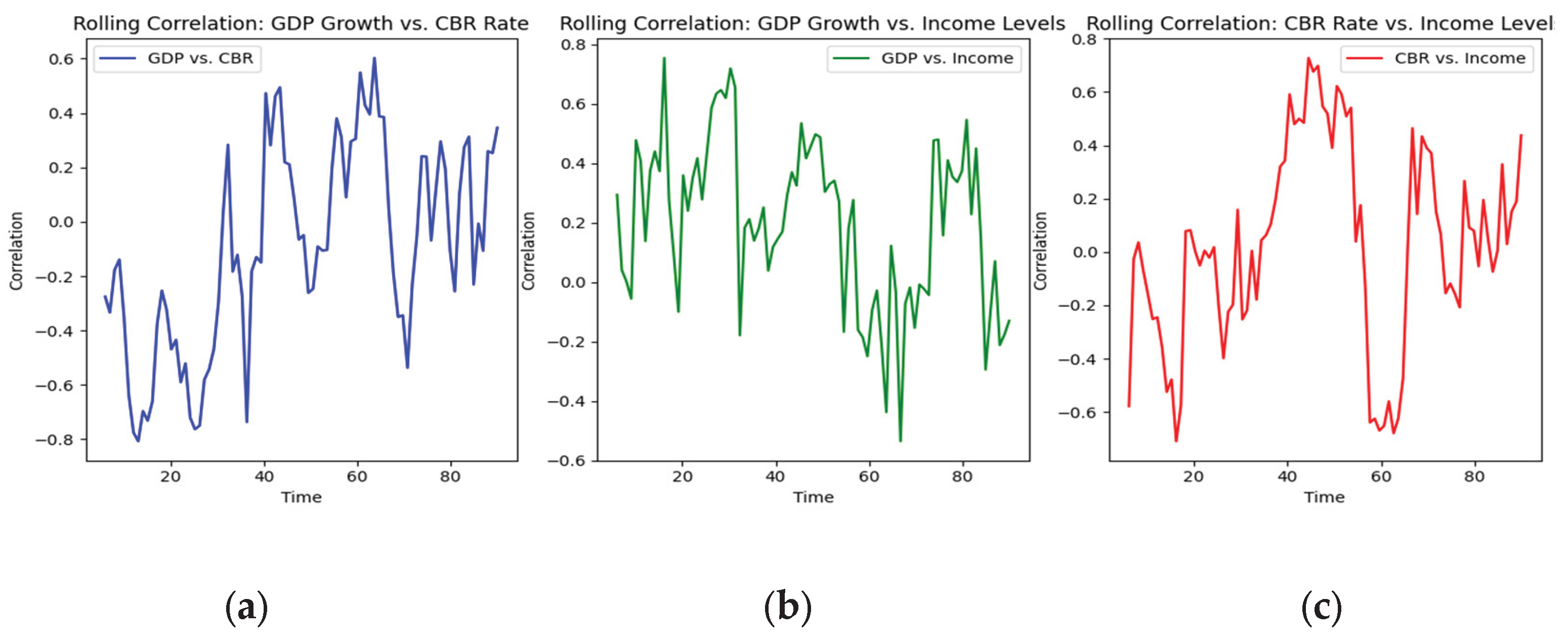
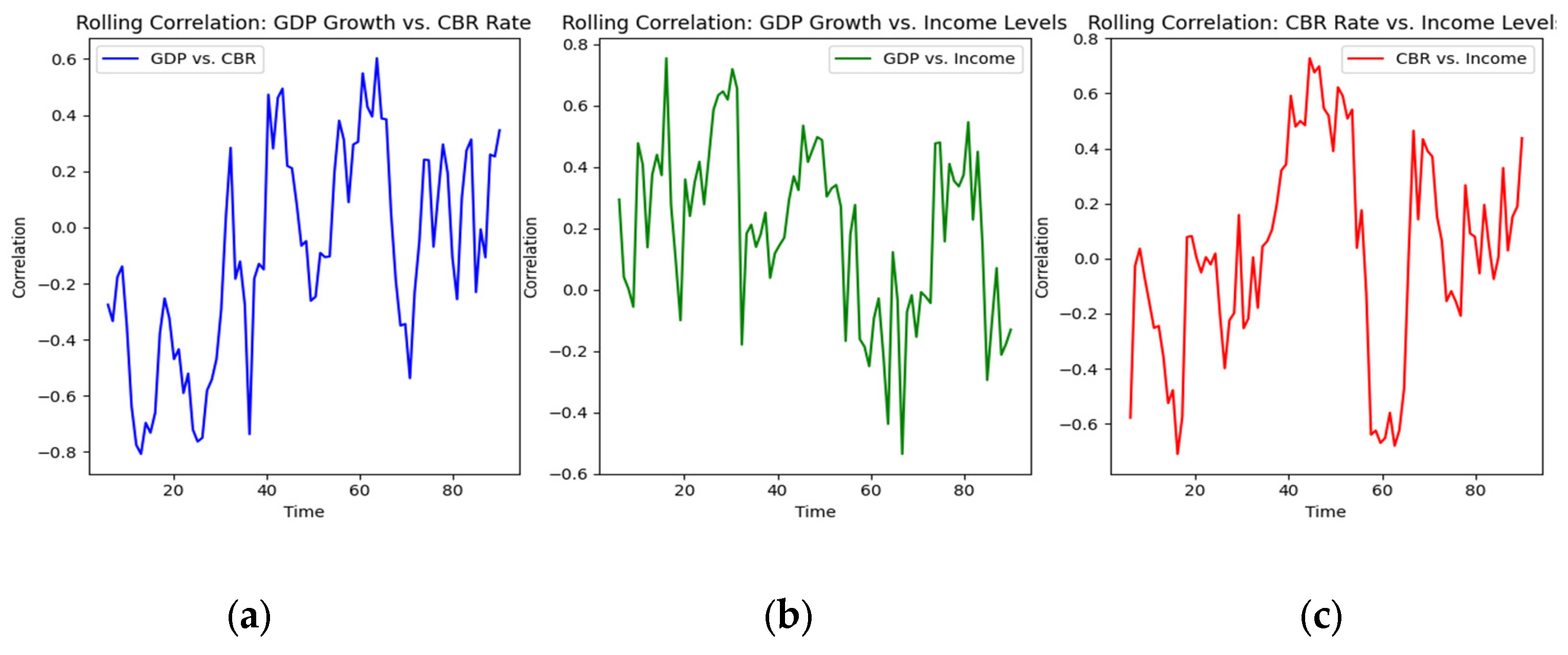
The correlation can be repeated over a distressed market such as that seen during the COVID pandemic, with sample data drawn from the US economy between February 2020 to May 2020. The data shows financial instruments exhibiting high levels of volatility of 46.56%, GDP Quarterly growth-rate of -1%, CBR rate of 3.35% p.a and a GDP per capita income of $60,000 [Source: Federal Reserve Bank of St. Louis]. The correlations here, observed over a 3 months window on unsecured loans (credit card loans over the same period) can be deduced as follows:

Table 2. The correlation matrix of the variational factors in a distressed market.

	GDP Growth	CBR Rate	Income Levels
GDP Growth	1.000000	-0.057004	0.122415
CBR Rate	-0.057004	1.000000	-0.009646
Income Levels	0.122415	-0.009646	1.000000

Table 2. The correlation matrix of the variational factors in a distressed market.

	GDP Growth	CBR Rate	Income Levels
GDP Growth	1.000000	-0.057004	0.122415
CBR Rate	-0.057004	1.000000	-0.009646
Income Levels	0.122415	-0.009646	1.000000

The figure below shows how the correlations between the three factors can be paired over the observation period of the declining market.

Figure 2. Distressed Market: Piecewise correlations (a) Between GDP and CBR rate, (b) GDP and Income, (c) CBR rate and Income.

Figure 2. Distressed Market: Piecewise correlations (a) Between GDP and CBR rate, (b) GDP and Income, (c) CBR rate and Income.

The corresponding Cholesky Decomposition factor L is given as follows:

Table 3. Cholesky Decomposition Matrix.

1.000000	0.00000	0.00000
-0.057004	1.000000	0.00000
0.122415	-0.0026722	0.9924754

Table 3. Cholesky Decomposition Matrix.

1.000000	0.00000	0.00000
-0.057004	1.000000	0.00000
0.122415	-0.0026722	0.9924754

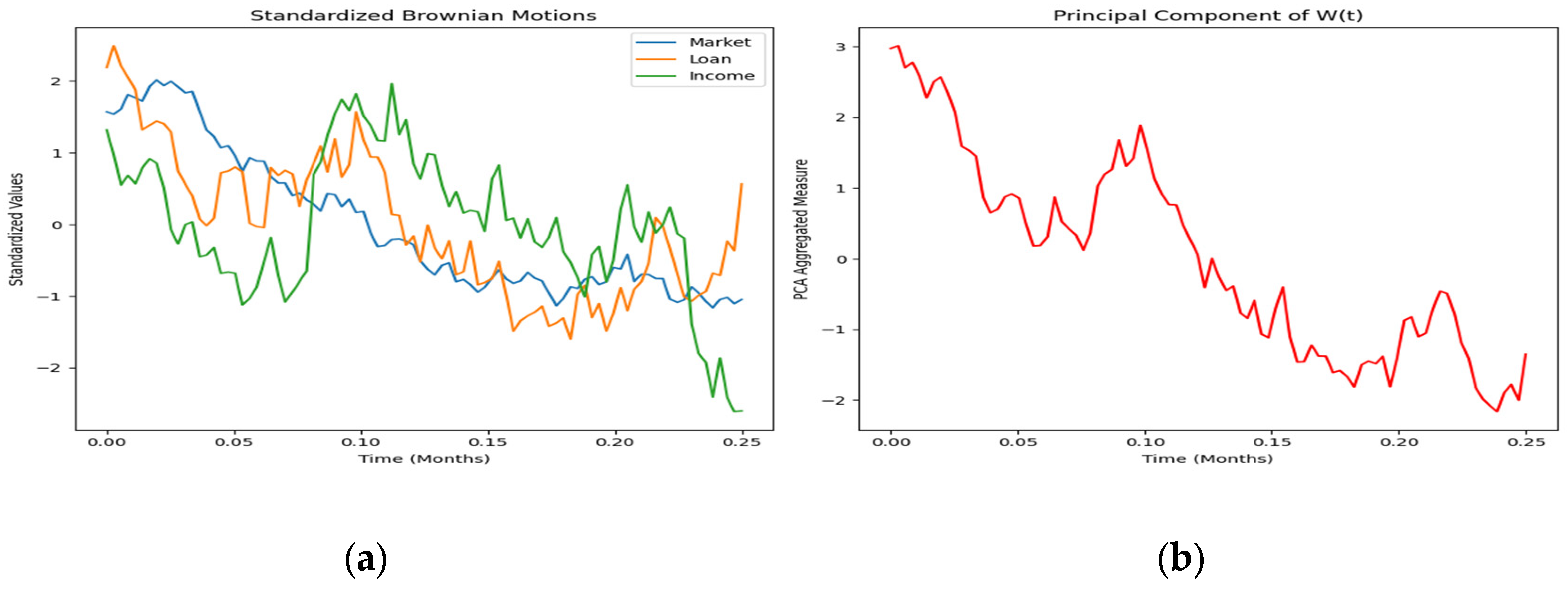
4.2. The Standardized and Aggregated Wiener Process

The three correlated Brownian motions can then be standardized to ensure that each factor contributes proportionately to the analysis. This ensures that our empirical process $u(x,t)$ is affected by a noise component in $\mathbb{R}$. Using PCA these components are collapsed into one aggregated measure $\dot{W}\left(t\right)$ whose value maximized the variance of the empirical process $u(x,t)$.

Figure 3. (a) Boom market standardized values of the Wiener process (September 2021 to December 2021) (b) Boom market aggregated values of the Wiener process under Principal component weighting (September 2021 to December 2021).

Figure 3. (a) Boom market standardized values of the Wiener process (September 2021 to December 2021) (b) Boom market aggregated values of the Wiener process under Principal component weighting (September 2021 to December 2021).

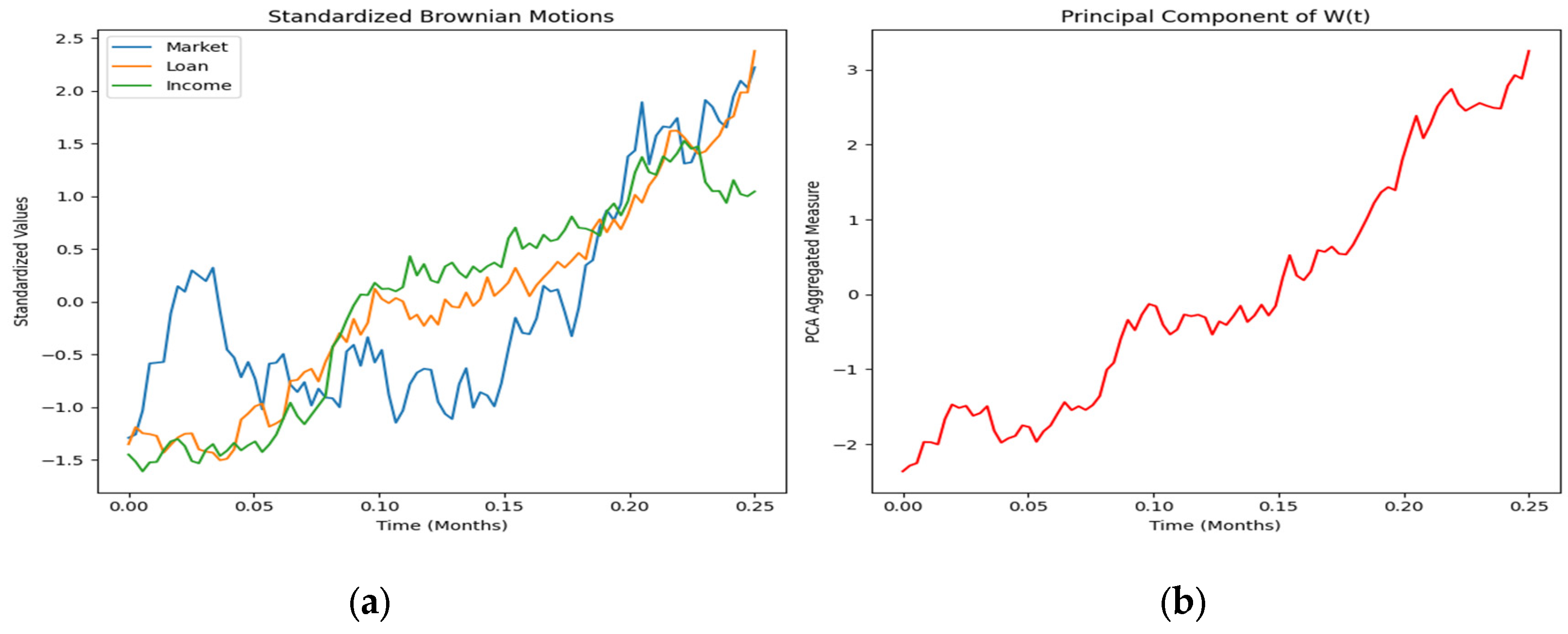
By combining the three: correlated GDP, CBR rate and income levels into one matrix and applying PCA, the model is able to capture the dominant trend of the market. The primary trend is extracted using linear regression by fitting the line of best fit that minimizes the sum of squared residuals, leaving the residuals to isolate short-term fluctuations from the overall trend. The noise aggregation yields a 85.279644% explained variance ratio.

Similar noise component standardization and aggregation can be extended to falling Covid pandemic market.

In Figure 4 above the distressed market parameters yield a 66.285134% explained variance ratio.

In both the booming and distressed markets, the PCA effectively aggregates the trends generated by the market GDP, loan Interest CBR rate, and Individual income indicators into a single principal component that encapsulates the economic outlook into one noise process.

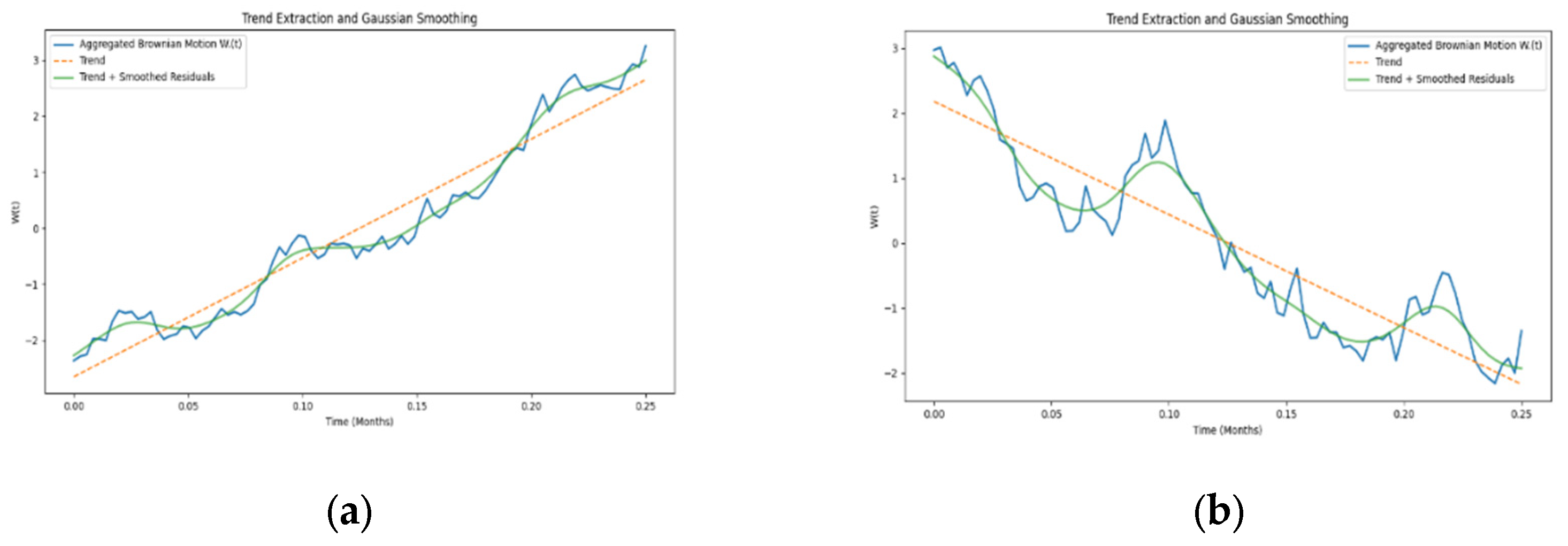
4.3. The Gaussian Kernel

The Gaussian Kernel convolution described in equation 19 and 20 can be used to load the aggregated noise described in figure 3 and 4 above with historical data effects to smoothen the noise by dampening the higher volatility while retaining the lower volatility points drawn from the three sources of variability.

In order to attain localized smoothing, Gaussian smoothing method is applied over the residuals using small standard deviations. Thus, minimizing the noise while preserving the crucial short-term movements.

Table 4. Gaussian Kernel parameters.

Parameter	Value in Boom Market	Value in Downward Market
Decay rate, $\lambda$	0.01	0.01

Table 4. Gaussian Kernel parameters.

Parameter	Value in Boom Market	Value in Downward Market
Decay rate, $\lambda$	0.01	0.01

The smoothened trend extracted Gaussian Kernel of the stochastic influence of the SPDE is done by overlaying a directional averaging over the smoothed principal component $\dot{W}\left(t\right)$ as shown below.

Figure 5. (a) Trend extracted and smoothened Gaussian Kernels under boom markets. (b) Trend extracted and smoothened Gaussian Kernels under distressed market.

Figure 5. (a) Trend extracted and smoothened Gaussian Kernels under boom markets. (b) Trend extracted and smoothened Gaussian Kernels under distressed market.

4.4. Mathematical Simulation and Analysis of the SPDE

In this section we will consider a practical use of the empirical measure to model the risk borne of unsecured loans.

We will proceed to simulate a case scenario where $u(x,t)$, is used to model the probability of default. However, the reader is guided that there are various sources of risk that a financial institution may want to mitigate as was mentioned in the literature review. The method of evaluating these risks is the same and can even be aggregated on the assumption of linearity and independence.

We proceed to formulate the probability of default as at time t as:

$$P_d\left(t\right)={\int }_{y_L}^{y_U}u(x,t|{\mathcal{F}}_t)dx$$

Where $u(x,t|{\mathcal{F}}_t)$ is the empirical density solving the SPDE with $x$ as the spatial point of credit worthiness instance such as credit score and, $y$ is density value of score limit such that

$$y:\{x\in [\mathrm{300,850}]⟶[\mathrm{0,1}\left]\right\}$$

where $y_L and y_U$represent transformed cutoff scores in a portfolio. This formulation provides a cumulative measure of default risk across a segment of the borrowers. The cutoffs​ are dynamically adjusted based on prevailing economic conditions or changes in lending policy.

Over time, $P_d\left(t\right)$ is analyzed to forecast trends in default probabilities, helping lenders anticipate shifts in the risk landscape and adjust their strategies to accommodate the changes in risk dynamics. By simulating the SPDE under different economic scenarios, businesses can predict how these factors might shift the distribution $u(x,t|{\mathcal{F}}_t)$ and thus $P_d\left(t\right)$.

Taking temporal partial derivative on $P_d\left(t\right),$ and substituting $u(x,t|{\mathcal{F}}_t)$ as defined in equation 20, we get the cumulative distribution of the bounded spatial probability of default

$${\displaystyle \frac{\partial }{\partial t}}{P}_d\left(t\right)={\displaystyle \frac{\partial }{\partial t}}{\int }_{y_L}^{y_U}\left\{({\sigma }^2\left(x,t\right){\displaystyle \frac{{\partial }^{2}u}{\partial x^2}}+\mu \left(x,t\right){\displaystyle \frac{\partial u}{\partial x}}+\eta \left(u, x,t\right){\dot{W}}_K\left(x,t\right))\left|{\mathcal{F}}_t\right)\right\}dx$$

We then analyze this probability of default from data drawn from the two contrasting economic conditions stated in section 4.1.

4.4.1. Euler-Maruyama Method on Probability of Default

To obtain the absolute probability of default, a finite difference scheme is utilized to handle the spatial derivatives while a time-stepping method like Euler-Maruyama for the temporal and stochastic components. We divide the range of FICO scores into discrete segments and the applying a time step small enough to capture the dynamics but large enough to ensure polynomial time computational efficiency.

To handle the stochastic term $\eta \left(u, x,t\right){\dot{W}}_K\left(x,t\right)$ we use Monte Carlo methods to simulate multiple paths of $u\left( x,t\right)$ under random influences, averaging the results to approximate $P_d\left(t\right)$.

Critical to the simulation’s success is the uniqueness of the FICO score ranges and time intervals in the discretization process into finite intervals. This discretization allows us to approximate the differential components of the SPDE, specifically the partial derivatives with respect to the FICO score, which represents the spatial dimension in our model. Similarly, the time dimension is discretized into steps that correspond to the duration over which we forecast the economic indicators and borrower behaviors. This step is crucial for tracing the evolution of default probabilities through time under various economic conditions.

Suppose we discretize the FICO score range $x$ into $N$ intervals with spacing $\Delta x$ and the time $t$ into $M$ intervals with spacing $\Delta t$.

Let $x_i=i\Delta x$ for $i=\mathrm{0,1},\dots ,N$ and $t_j=j\Delta t$ for $j=\mathrm{0,1},\dots ,M$. The value of $u$ at these points is denoted as $u_i^j=u(x_i,t_j)$. The Dirichlet boundary conditions specifying the state variable $u(x,t)$ at the boundaries $x_0$ (minimum FICO score) and $x_N$(maximum FICO score) for all time points of the spatial and temporal domains.

Setting the borrowers with the lowest FICO score have a very high default probability, possibly approaching 1

$$u_o^j=u\left(x_0,t_j\right)=1$$

and the borrowers with the highest FICO score have a very low default probability, which might be close to 0.

$$u_N^j=u\left(x_N,t_j\right)=0$$

These boundary conditions, when rigorously implemented, help maintain stability by preventing boundary-induced anomalies in the numerical solution. Ensuring that the initial conditions $u_o^j$ ​ are smooth and consistent with the boundary conditions at $x_0$ ​ and $x_N$​ is crucial for the physical realism of the model.

For the internal nodes $i=\mathrm{0,1},\dots ,N-1$, the updated SPDE equation written in FDM with time derivatives becomes:

$$u_i^{j+1}=u_i^j+\left[{\sigma \left(u_i^j,x_i,t_j\right)}^2\left\{{\displaystyle \frac{u_{i+1}^j-2u_i^j+u_{i-1}^j}{{\left(\Delta x\right)}^2}}\right\}+\mu \left(u_i^j,x_i,t_j\right)\left\{{\displaystyle \frac{u_{i+1}^j-u_{i-1}^j}{2\Delta x}}\right\}\right]\Delta t+\eta \left(u_i^j,x_i,t_j\right){\xi }_i^j\sqrt{\Delta t}$$

where ${\displaystyle \frac{\partial u}{\partial t}}{|}_{(x_i,t_j)}\approx {\displaystyle \frac{u_i^{j+1}-u_i^j}{\Delta t}}$, ${\displaystyle \frac{\partial u}{\partial x}}{|}_{(x_i,t_j)}\approx {\displaystyle \frac{u_{i+1}^j-u_{i-1}^j}{2\Delta x}}$ and ${\displaystyle \frac{{\partial }^{2}u}{\partial x^2}}{|}_{(x_i,t_j)}\approx {\displaystyle \frac{u_{i+1}^j-2u_i^j+u_{i-1}^j}{{\left(\Delta x\right)}^2}}$ respectively.

While the stochastic colored noise term is approximated using the Gaussian random variable ${\xi }_i^j$ scaled appropriately such that

$\eta \left(u, x_i,t_j\right){\dot{W}}_K\left(x_i,t_j\right)\left|{\mathcal{F}}_t\right)\Delta t\approx \eta \left(u_i^j,x_i,t_j\right){\xi }_i^j\sqrt{\Delta t}$The model equation in this case depends on the parameters presented on a particular market condition and a given scoring criterion. For example, the SPDE below is drawn from a boom market and the borrowers of score range 500 to 750.

$${\displaystyle \frac{\partial u}{\partial t}}=0.035{\displaystyle \frac{{\partial }^{2}u}{\partial x^2}}+0.05{\displaystyle \frac{\partial u}{\partial x}}+0.03\dot{W}\left(x,t\right) \mathrm{w}\mathrm{i}\mathrm{t}\mathrm{h}\mathrm{i}\mathrm{n}\mathrm{i}\mathrm{t}\mathrm{i}\mathrm{a}\mathrm{l}\mathrm{c}\mathrm{o}\mathrm{n}\mathrm{d}\mathrm{i}\mathrm{t}\mathrm{i}\mathrm{o}\mathrm{n} u\left(x,0\right)=0.07$$

4.4.2. Boom Market Evolution of Probability of Default Using SPDE Approach

A boom market is characterized by stability in credit market, improved borrower creditworthiness, and stable low lending rates. Such an economy is also characterized by a positive GDP growth rate, low CBR rates and increased household income.

The SPDE parameters in a boom market exhibit significantly low volatility, σ, reflecting a reduced uncertainty; with higher mean rate of borrowing, μ, reflecting optimism in repayment capabilities. Moderate levels of $\eta$, implying lower unexpected economic shocks.

To effectively manage and anticipate credit risk from an unsecured loan portfolio, particularly within the context of a stable economy, a Monte Carlo simulation approach is employed, leveraging extensive historical economic data to capture default probabilities.

Given the economic scenario described in section 4.1 and portfolio historical data drawn from 200,000 borrowers, the drift coefficient μ of 0.16 indicating improved credit lending metrics such as credit scores. The diffusion coefficient σ=0.01. A reflection of reduced uncertainty in borrowers’ credit worthiness. The Economic factors influencing the stochastic component (η=0.005) over the observation period remain as described in section 4.1 above. All the parameters are taken as deterministic over the observation duration.

This simulation of the default probability based on FICO range can give an insight into the risk borne from various Scores in various market conditions.

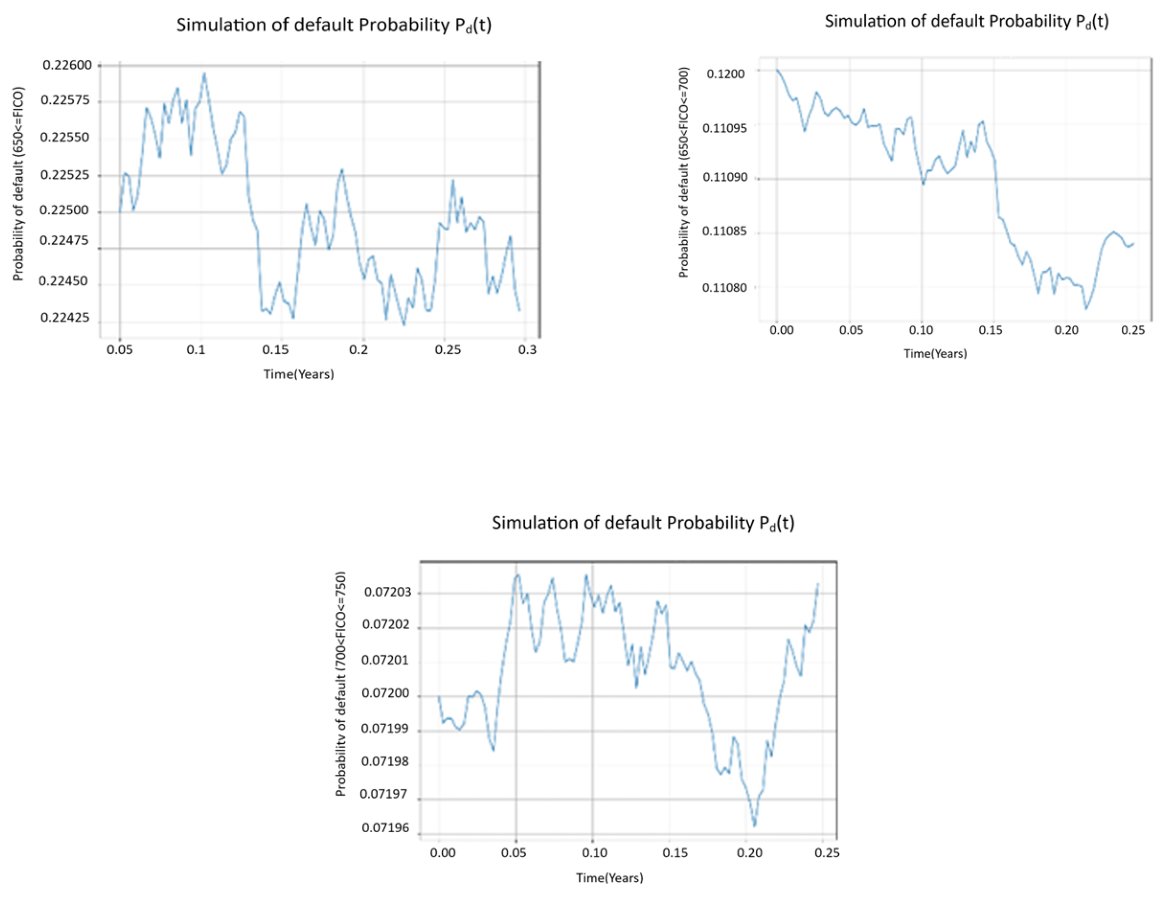
Fig 6 shows the probabilities of defaults in the three score categories in a boom market characterized by cheap credit. Borrowers with credit score of less than 650 have a higher probability of default over the three months observational period compared to borrowers with credit scores above 650.

Table 5. SPDE Simulation Parameters in a boom market.

Parameters	FICO ≤ 650	FICO Range 650 <FICO ≤700	FICO Range 700 <FICO ≤750
mu	0.05	0.08	0.16
sigma	0.35	0.20	0.14
eta	0.03	0.009	0.004
M	100	50	50
N	90	90	90
$u\left(x,0\right)$	0.2250	0.1200	0.0720

Table 5. SPDE Simulation Parameters in a boom market.

Parameters	FICO ≤ 650	FICO Range 650 <FICO ≤700	FICO Range 700 <FICO ≤750
mu	0.05	0.08	0.16
sigma	0.35	0.20	0.14
eta	0.03	0.009	0.004
M	100	50	50
N	90	90	90
$u\left(x,0\right)$	0.2250	0.1200	0.0720

Figure 6. Evolution of probability of default in a boom market under different credit score tranches.

Figure 6. Evolution of probability of default in a boom market under different credit score tranches.

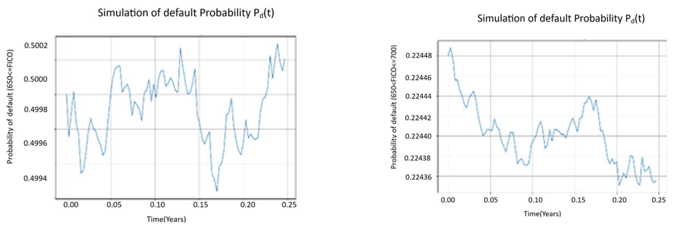
4.4.3. Probability of Default in a Distressed Market

In a distressed market, the credit market witnesses heavy default rates with the heaviest losses experienced in score category with FICO ≤ 650. The volatility level is also higher in the lower score category. The stochastic influence coefficient also shows a significant contribution to the SPDE.

Table 6. SPDE Simulation Parameters in a distressed market.

Parameters	FICO ≤ 650	FICO Range 650 <FICO ≤700	FICO Range 700 <FICO ≤750
mu	0.03	0.05	0.09
sigma	0.55	0.33	0.21
eta	0.33	0.17	0.10
M	100	50	50
N	90	90	90
$u\left(x,0\right)$	0.5000	0.1743	0.1250

Table 6. SPDE Simulation Parameters in a distressed market.

Parameters	FICO ≤ 650	FICO Range 650 <FICO ≤700	FICO Range 700 <FICO ≤750
mu	0.03	0.05	0.09
sigma	0.55	0.33	0.21
eta	0.33	0.17	0.10
M	100	50	50
N	90	90	90
$u\left(x,0\right)$	0.5000	0.1743	0.1250

Figure 7. Evolution of probability of default in a distressed market under different credit scores.

Figure 7. Evolution of probability of default in a distressed market under different credit scores.

Analyzing the risk for each FICO score segment based on their default probabilities over time provides crucial insights, particularly in a recovery economy scenario. For the Low-Risk Segment (FICO > 700), default probabilities remain consistently low, demonstrating minor sensitivity to economic fluctuations. This stability likely stems from higher financial reserves, better credit access, and stable employment conditions characteristic of such borrowers. Lenders should focus on retaining these low-risk clients by maintaining competitive interest rates and offering premium financial products, leveraging their reliability for stable returns.

The Medium-Risk Segment (650 < FICO ≤ 700) exhibits more variability in default probabilities than the low-risk segment, with a noticeable response to economic downturns. The financial health of these borrowers often correlates directly with prevailing economic conditions, such as employment rates and GDP growth. They face a higher risk of default under adverse economic conditions but can recover if supported appropriately. To manage this risk, lenders should monitor economic indicators closely and consider flexible loan terms and refinancing options during economic recoveries to help sustain these borrowers' creditworthiness.

In contrast, the High-Risk Segment (FICO ≤ 650) shows the highest and most volatile default probabilities, which sharply increase during economic downturns. This segment's financial stability is extremely sensitive to economic stress, often exacerbated by lower savings, precarious employment, or high debt-to-income ratios. For these borrowers, lenders should employ stringent risk assessment measures, potentially requiring higher reserves or significant collateral to mitigate risks. Additionally, dynamic risk-based pricing might be appropriate, where interest rates adjust in response to real-time changes in the borrowers' risk profiles, ensuring that lending practices adequately reflect the heightened risk associated with this segment.

A rigorous sensitivity analysis can be conducted on key parameters such as diffusion (σ), drift (μ), and stochastic influence (η). This analysis helps to understand how susceptible the default probabilities are to changes in these parameters and allows for adjustments to reflect different rates of economic recovery or potential downturns.

The culmination of this process is a detailed report that not only summarizes the simulation process and findings but also offers actionable recommendations for stakeholders. This report includes strategic risk management approaches designed to mitigate potential future risks based on the simulation results.

5. Discussions

In this section, we summarize the key findings of the study, then discuss their implications for real-world unsecured lending, and suggest avenues for future research. The primary goal of this paper was to develop a novel SPDE-based framework for modeling the wealth dynamics of unsecured loans, and the results have demonstrated both the feasibility and advantages of this approach in evaluating the probability of default.

5.1. Summary of Findings

Through the construction of a stochastic partial differential equation model, we have shown that it is possible to capture the evolution of a loan portfolio’s wealth, its loss and default risk under the influence of multiple correlated factors. Starting from an individual loan’s stochastic wealth process driven by borrower-specific, loan-specific, and macroeconomic shocks, we derived a measure-valued process representing the entire portfolio. Using a combination of probability limit theorems and stochastic analysis, we proved that as the number of loans grows large, the empirical distribution of loan states converges to a deterministic function, $u(x,t)$, that satisfies a well-posed SPDE. This SPDE incorporates drift terms reflecting average economic trends and diffusion terms capturing the volatility due to random shocks, underpinned by a Gaussian kernel to account for temporal persistence (market memory) in those shocks. We validated the model with numerical simulations, demonstrating how it can predict the probability of default (PD) for different segments of borrowers over time. For example, in a stable “boom” economic scenario, default probabilities remained low across all credit score segments, whereas in a stressed “crisis” scenario, the lower-credit segments showed a sharp increase in PD. These outcomes are consistent with real-world expectations, lending credibility to the model.

5.2. Real-World Applications

The SPDE model introduced in this study provides a robust tool for various stakeholders in the financial industry. Financial institutions (banks, credit lenders) can use the model to simulate and forecast default rates under different economic conditions. Because the model incorporates correlated macroeconomic factors (like GDP growth and interest rates) and borrower behavior, it can be used for stress testing an unsecured loan portfolio. For instance, risk managers could simulate a sudden economic downturn by introducing a shock to the drift or volatility terms and observe how the distribution of borrower wealth evolves. The model would yield the changing probability of default over time, helping in predicting risky segments of the portfolio. This allows for proactive policy changes that might help in mitigating the adversities of such scenarios, such as adjusting credit limits, pricing for risk, or bolstering reserves.

Another real-world application of the proposed model above is in loan pricing and valuation. Lenders could also integrate this model into pricing unsecured loan products. By understanding the stochastic evolution of borrower wealth and default likelihood, lenders can more accurately price the risk premium on loans. The SPDE’s solution $u(x,t)$, gives the distribution of “financial health” scores over time. Through its derivation, expected losses can be computed and use those to inform interest rates or insurance for loan portfolios.

Regulatory bodies and policymakers can benefit from the model as a means to gauge the health of the unsecured lending market. Since unsecured loans (like credit card debt, student loans, mobile applications loans, etc.) have no collateral, they pose a higher risk to the financial system in times of stress. Our model, when calibrated to market data, can serve as an early warning system. If, for example, the model predicts a rising wave of defaults given certain macroeconomic forecasts, regulators might tighten lending standards or increase capital requirements for those exposures. The model’s ability to track the distribution of loans is especially useful for systemic risk analysis, as it can capture concentration of risk (e.g., if many borrowers are at the brink of default simultaneously).

Notably, from a policy implications perspective, the findings highlight how macroeconomic stability translates into lower default risk for unsecured loans. This underscores the importance of policies that maintain economic growth and employment – benefits that clearly trickle down to consumer credit stability. Conversely, in a downturn, our results suggest that interventions might be needed to assist the most vulnerable borrower segments.

5.3. Implications of the SPDE Approach

By introducing a dual perspective of spatial dimension (the “creditworthiness” axis, which can be thought of as a transformed credit score or wealth metric) and a temporal dimension, the SPDE approach enriches traditional credit risk models. Unlike static credit scoring or even simpler stochastic loss models, the SPDE captures dynamics and interdependence. At its core, it shows how shocks propagate through the borrower population over time. One key implication is that credit risk is not memoryless – past economic events leave a lingering effect (modeled by the Gaussian kernel’s decay of influence). This supports the idea that regulatory stress tests and economic policy should consider not just point-in-time metrics but also the path of how we got there. Prolonged period of sustained growth can build resilience, whereas steep down markets can lead to shocks that can compound dramatically into risk of default over a sustained period. Our model provides a quantitative way to describe these phenomena.

5.4. Future Research Directions

This work opens several avenues for further investigation. The model can be extended to incorporate more factors and in higher dimensions. Future models could include more granular economic factors or borrower attributes. For example, segmenting by different loan types (credit cards, student loans, personal loans and mobile application loans) might require a multi-dimensional state space or a system of coupled SPDEs. Incorporating factors like employment status or debt-to-income ratio as additional dimensions could provide a more detailed picture of risk, albeit at the cost of analytical tractability.

The complex, non-linear nature of the SPDE might benefit from machine learning techniques. One could use historical loan performance data to train the drift and diffusion functions rather than assuming functional forms. Techniques from reinforcement learning or neural SPDE solvers could calibrate the model in real-time, as economic conditions change. A hybrid model where the SPDE provides the structure and machine learning provides data-driven calibration could be very powerful.

Solving SPDEs can be computationally intensive. Our use of Euler-Maruyama and finite differences is straightforward but may not be the most efficient. Future research could explore advanced numerical schemes or variance reduction techniques for the Monte Carlo simulation of the SPDE. Ensuring stability and convergence of the numerical method for a wide range of parameters (especially in extreme stress scenarios) would be important for practical adoption.

Researchers might apply this SPDE model to real loan portfolio data from banks to validate its predictive performance. A comparative study between this SPDE approach and traditional credit risk models such as logistic regression, survival analysis, or agent-based simulations, would shed light on how much gain in accuracy or insight the SPDE provides. It would be interesting to see, for instance, if the SPDE model could have foreseen the rise in unsecured loan defaults during an event like the COVID-19 pandemic more clearly than standard models.

6. Conclusions

In conclusion, this paper introduced a Stochastic PDE model for unsecured loan wealth dynamics and demonstrated its theoretical soundness and practical relevance. The model bridges individual loan behavior and portfolio-level risk through a continuous, stochastic description that accounts for both idiosyncratic noise and correlated economic shocks. Our theoretical analysis confirmed that the model is mathematically well-behaved (admitting a unique solution that remains stable over time), and the numerical experiments illustrated how it can be applied to estimate default probabilities under various economic conditions. The SPDE approach provides a unifying framework to analyze credit risk in unsecured lending, offering insights that are valuable to both financial institutions and regulators.

Ultimately, by capturing the spatial-temporal evolution of credit risk, the model contributes to a deeper understanding of how shocks and policies propagate through loan portfolios. We believe that with further refinement and calibration, such models can become integral to risk management strategies and policy decision-making, helping to ensure stability in the ever-growing unsecured credit markets. The work presented here is a step in that direction, laying the groundwork for more sophisticated and inclusive models in future research.

References

- Ahmad, R., Hambly, B. M., & Ledger, S. (2018). A stochastic partial differential equation model for the pricing of mortgage-backed securities. Stochastic Processes and their Applications, 128(6), 1938-1977.
- Altman, E. I. (1968). Financial ratios, discriminant analysis, and the prediction of corporate bankruptcy. The Journal of Finance, 23(4), 589-609.
- Black, F., & Scholes, M. (1973). The pricing of options and corporate liabilities. Journal of Political Economy, 81(3), 637-654.
- Cont, R., & Minca, A. (2013). Recovering portfolio default intensities implied by CDO quotes. Mathematical Finance, 23(1), 94-121.
- Duffie, D., & Singleton, K. J. (1999). Modeling term structures of defaultable bonds. Review of Financial Studies, 12(4), 687-720.
- Fan, J., & Yao, Q. (2003). Nonlinear time series: Nonparametric and Parametric Methods. Springer.
- Filipović, D. (2009). Term-Structure Models: A Graduate Course. Springer.
- Fouque, J.-P., & Langsam, J. (2013). Handbook on Systemic Risk. Cambridge University Press.
- Hao Tang, Feng-Yu Wang (2023). A General Framework for Solving Singular SPDEs with Applications to Fluid Models Driven by Pseudo-differential Noise.
- Hand, D. J., & Henley, W. E. (1997). Statistical classification methods in consumer credit scoring: A review. Journal of the Royal Statistical Society: Series A (Statistics in Society), 160(3), 523-541.
- Piterbarg, V. (2006). A multi-factor, non-linear, stochastic volatility model. Quantitative Finance, 6(6), 555-568.
- Swishchuk, A. (2017). Modeling and Pricing of Swaps for Financial and Energy Markets with Stochastic Volatilities. Cambridge University Press.
- Erica Xuewei Jiang, Gregor Matvos, Tomasz Piskorski & Amit Seru (2023). National Bureau of Economic Research (NBER). Monetary Tightening and Its Impact on Bank Asset Valuation.
- Timo Löyttyniemi (2023). Centre for Economic Policy Research (CEPR). Financial Instabilities in Banking and Derivatives Markets During 2022-2023.
- Alexander, C. (2019). Market Risk Analysis. Wiley.
- Baxter, M., & Rennie, A. (2016). Financial Calculus: An Introduction to Derivative Pricing. Cambridge University Press.
- Brigo, D., & Mercurio, F. (2006). Interest Rate Models - Theory and Practice: With Smile, Inflation and Credit. Springer.
- Carmona, R. (2009). Indifference Pricing: Theory and Applications. Princeton University Press.
- Chapelle, A. (2019). Operational Risk Management. Wiley.
- Chen, Z., Wang, Y., & Li, H. (2019). Macroeconomic Indicators and Personal Investment Decisions: Evidence from Emerging Markets. Journal of Economic Behavior & Organization, 165, 36-49.
- Duffie, D., & Singleton, K. J. (2012). Credit Risk: Pricing, Measurement, and Management. Princeton University Press.
- Fouque, J.-P., Papanicolaou, G., Sircar, R. K., & Solna, K. (2011). Multiscale Stochastic Volatility for Equity, Interest Rate, and Credit Derivatives. Cambridge University Press.
- Glasserman, P. (2004). Monte Carlo Methods in Financial Engineering. Springer.
- Hull, J. (2015). Risk Management and Financial Institutions (4th ed.). Wiley.
- Jarrow, R., & Turnbull, S. (2015). Credit Risk Models and the Management of Risk. Journal of Finance, 53(2), 507-530.
- Lee, H., & Kim, S. (2018). Impact of Loan Terms on Borrower Risk: A Dynamic Analysis. Finance Research Letters, 26, 142-150.
- Li, Z., & Wong, T. J. (2018). Information Dissemination Through Embedded Financial Analysts: Evidence from China. Journal of Financial Economics, 130(3), 653-677.
- Löffler, G., & Posch, P. N. (2011). Credit Risk Modeling using Excel and VBA. Wiley.
- Nguyen, T. (2021). Calibration Techniques for Stochastic Differential Equations in Financial Markets. Computational Economics, 58(4), 983-1005.
- Rogers, L. C. G., & Williams, D. (2017). Diffusions, Markov Processes, and Martingales: Volume 2, Itô Calculus. Cambridge University Press.
- Shreve, S. E. (2004). Stochastic Calculus for Finance II: Continuous-Time Models. Springer Finance.
- Smith, J., & Jones, A. (2020). Personal Financial Management and Wealth Accumulation: An Analytical Approach. Journal of Financial Studies, 45(3), 223-241.
- Wilmott, P. (2010). Paul Wilmott Introduces Quantitative Finance. Wiley.
- Balcilar, M., Gupta, R., & Miller, S. M. (2018). Dynamic correlations between oil prices and inflation in South Africa. Journal of Economic Studies.
- Ballotta, L., & Bonfiglioli, E. (2016). Factor model for Lévy processes: Systematic and specific risk components in asset dynamics. Quantitative Finance.
- Chiang, T. C., Jeon, B. N., & Li, H. (2007). Dynamic correlation analysis of financial contagion: Evidence from Asian markets. Journal of International Money and Finance.
- Da Fonseca, J., Grasselli, M., & Tebaldi, C. (2007). Option pricing when correlations are stochastic: An analytical framework. Review of Derivatives Research.
- Fernández, A., Osajima, Y., & Fornari, F. (2013). Bounded functions in SABR models. Finance Research Letters.
- Junior, P. H., & Franca, I. D. P. (2012). Dynamic correlations and volatility linkages between stocks and sovereign bonds: Evidence from the European region. Finance Research Letters.
- Langnau, A. (2010). Dynamic correlation models: Modeling r as a function of stochastic state processes. Journal of Financial Econometrics.
- Osajima, Y. (2007). Theoretical implications of bounded functions in financial modeling. Journal of Financial and Quantitative Analysis.
- Syllignakis, M. N., & Kouretas, G. P. (2011). Dynamic correlation analysis of financial contagion in Europe. International Review of Economics & Finance.
- Teng, L., Meissner, G., & Ma, L. (2016). The Jacobi process in bounded stochastic processes with financial applications. Mathematical Finance.
- Van Emmerich, A. (2006). Stochastic models for r: Bounded functions of stochastic state processes in derivatives pricing. Journal of Banking & Finance.
- Wang, M. Y. (2009). Correlated variance gamma processes by Brownian motions with constant correlation. Journal of Financial Econometrics.
- Xiong, X., Wang, S., & Hu, J. (2018). Time-varying correlation between policy index and stock returns in China. China Economic Review.
- Zhou, C., & Yin, G. (2003). Markov processes in regime-switching models for stochastic local correlation. Mathematical Finance.
- Onno Eberhard, Thibaut Cuvelier, Michal Valko, and Bruno De Backer(2023). Middle-Mile Logistics Through the Lens of Goal-Conditioned Reinforcement Learning. NeurIPS Workshop on Goal-Conditioned Reinforcement Learning.
Figure 4.
(a) Distressed market standardized values of the Wiener process (February 2020 to May 2020) (b) Distressed market aggregated values of the Wiener process under Principal component weighting (February 2020 to May 2020).
Disclaimer/Publisher’s Note: The statements, opinions and data contained in all publications are solely those of the individual author(s) and contributor(s) and not of MDPI and/or the editor(s). MDPI and/or the editor(s) disclaim responsibility for any injury to people or property resulting from any ideas, methods, instructions or products referred to in the content. |
© 2025 by the authors. Licensee MDPI, Basel, Switzerland. This article is an open access article distributed under the terms and conditions of the Creative Commons Attribution (CC BY) license (http://creativecommons.org/licenses/by/4.0/).
Copyright: This open access article is published under a Creative Commons CC BY 4.0 license, which permit the free download, distribution, and reuse, provided that the author and preprint are cited in any reuse.