
Submitted:
21 July 2025
Posted:
23 July 2025
You are already at the latest version
Abstract
Recent advances in plant electrophysiology and machine learning suggest that bioelectric signals in plants may encode environmentally relevant information beyond physiological processes. In this study, we present a novel framework to analyse waveforms from real-time bioelectrical potentials recorded in vascular plants. Using a multi-channel electrophysiological monitoring system, we acquired continuous data from Vitis vinifera samples in a vineyard plantation under natural conditions. Plants were in different health conditions, from healthy, to under the infection of flavescence dorée, to plants in recovery from the same disease, to dead stumps. These signals were used as input features for an ensemble of complex machine learning models, including recurrent neural networks, trained to infer short-term meteorological parameters such as temperature and humidity. The models demonstrated predictive capabilities with accuracy comparable to sensor-based benchmarks between one and two degree Celsius for temperature, particularly in forecasting rapid weather transitions. Feature importance analysis revealed plant-specific electrophysiological patterns that correlated with ambient conditions, suggesting the existence of biological pre-processing mechanisms sensitive to microclimatic fluctuations. This bioinspired approach opens new directions for developing plant-integrated environmental intelligence systems, offering passive, and biologically rooted strategies for ultra-local forecasting—especially valuable in remote, sensor-sparse, or climate-sensitive regions. Our findings contribute to the emerging field of plant-based sensing and biomimetic environmental monitoring, expanding the role of flora from passive observers to active participants in Earth system observation.
Keywords:
Vitis vinifera
; bioelectric potential
; electrophysiology
; machine learning
; weather forecast
; bioinspiration
1. Introduction
The increasing demand for high-resolution, real-time weather forecasting has catalyzed the exploration of unconventional data sources and methodologies. Traditional meteorological models, while robust, often lack the granularity required for hyper-local predictions, especially in heterogeneous terrains and microclimates. In turn, weather forecasting can be profitably used to predict crop yield by exploiting similar ML tools [1]. The link between meteorology and biology extends to the scale of the predictive models, and represents a profound connection between two apparently detached fields [2]. Recent advancements in plant electrophysiology suggest that plants, through their bioelectrical signals, may serve as sensitive indicators of environmental changes, offering a novel avenue for localized weather forecasting [3]. Plants exhibit a range of electrical activities in response to environmental stimuli, including variations in temperature, humidity, light intensity, and mechanical stress [4]. These bioelectrical responses [5], encompassing action potentials and variation potentials, are integral to plant signaling mechanisms and have been documented to reflect external environmental conditions [6]. The potential of these signals as proxies for environmental monitoring has been further underscored by studies demonstrating their correlation with specific abiotic stressors [7,8].
The integration of machine learning (ML) techniques with plant electrophysiological data has opened new frontiers in environmental sensing. ML algorithms, particularly deep learning models, have shown proficiency in deciphering complex, non-linear patterns within bioelectrical signals, enabling the classification and prediction of various environmental parameters [9]. For instance, supervised ML models have been employed to predict vines water status based on electrophysiological inputs, achieving notable accuracy [10]. In another study, machine learning algorithms (Artificial Neural Networks, Convolutional Neural Network, Optimum-Path Forest, k-Nearest Neighbors and Support Vector Machine) have been combined with Interval Arithmetic, and findings showed that Interval Arithmetic and supervised classifiers are more suitable than deep learning techniques [11].
Building upon this foundation, the present study explores the feasibility of utilizing plant bioelectrical signals as inputs for ML models aimed at forecasting local weather conditions. By harnessing the innate sensitivity of plants to their immediate environment, we propose a biomimetic approach to weather prediction that complements existing meteorological methods. This interdisciplinary endeavor aligns with the principles of biomimetics, wherein biological systems inspire innovative technological solutions.
The objectives of this research are threefold: (1) to establish a reliable methodology for recording and processing plant bioelectrical signals in situ; (2) to develop and train ML models capable of translating these signals into accurate short-term weather forecasts; and (3) to evaluate the performance of these models against conventional forecasting techniques. Through this study, we aim to contribute to the development of sustainable, plant-based environmental monitoring systems that enhance the precision of local weather forecasting.
2. Materials and Methods
2.1. Experimental Setup and Data Statistics
A traditional vineyard plant was selected to perform this study, as shown in Figure 1. It is located in Vigliano d’Asti, Monferrato, Italy (Cantina Adorno). For the collection of bioelectric potentials, two needle electrodes (MN4022D10S subdermal electrodes from SPES MEDICA SRL, Italy) 0.4 mm diameter, 22 mm in length were used to contact each plant by puncturing the bark. They were positioned 1 cm apart, and connected using double shielded ultra low resistance cable INCA1050HPLC (MD, Italy) for high fidelity audio application to a DI-710-US data logger (DATAQ Instruments, Akron, U.S.A.), used in differential channel mode, recording at a frequency of 1 Sample/s per channel, with 16 bit resolution and 1000 mV of voltage range. The maximum cable length was 5.2 m, adding an additional resistance component of 36 ± 2 m, an additional capacitance component of 78 ± 2pF and an additional inductive component of 78 ± 400nH . The cable structure is composed by an inner copper core, a first polyethylene dielectric insulation, a second semiconductive insulation, a third metallic net shield with coverage of 90%, and a final polyvinylchloride flexible coverage. The presence of the semiconductive insulation between the dielectric one and the net shield allows to discharge accumulated charges due to triboelectrification by cable movements, generally responsible for additional noise. The ideal electrical connection scheme is shown in the inset of Figure 1. Local climatic data was provided by a probe station (Primo Principio S.r.l., Italy). The eight plants object of this study were selected as statistically representative of the entire plantation, a high density vineyard. Furthermore a logistic aspect was considered in the choice of the sample, with close plants allowing the use of a single recording device connected by the shortest possible cables, to avoid signal corruption by long transmission lines. The input from dead, affected, as well as healthy plants is considered to be equally important. The plants’ health status is determined on the basis of manned observation by agronomers. Here the discriminant is the action induced on the plants by Flavescence dorée, which has become an endemic disease in the Monferrato area where the vineyard is located, therefore their symptoms as well as the aspect of a plant that survives to the phytoplasm and recovers until fruiting again, are very well known. The causal agent of Flavescence dorée is a phytoplasm belonging to the group of grapevine yellows, which colonizes the host’s phloem tissues and causes blockage of the elaborated sap, triggering an imbalance in the plant’s physiological activities. In late-stage manifestations, the grape clusters progressively shrivel and may partially or completely dry out; in cases of early symptom onset, infected shoots appear gummy in texture and tend to bend downwards, giving the plant a prostrate appearance [12]. It first appeared in 2000. Unfortunately there is no known remedy for the Flavescence dorée, the current action taken by farmers and enforced by local governments, consists in spreading insecticides that should terminate Scaphoideus titanus, known as being responsible for the spreading of the disease. Recovery occurs as a combination of agronomic actions (pruning infected branches) and eventually of plant reinforcement through other branches. This process typically requires 3 to 4 years before a fruiting season appears, of course unless the plant dies in between. After infection, the plants develop a very peculiar structure: even after recovery the signs of Flavescence dorée can be recognized, as their bark becomes more permeable, fragile, while healthy plants preserve a neat structure. Therefore by healthy plants we mean individuals which have never been infected, by plants under recovery we mean individuals infected between 1 and 4 years before, too sick to bear fruits at all, and by fully recovered plants that have produced fruits we mean individuals infected between 20 and 4 years before. Collection site `A’ represents a plant under recovery phase with no fruits yet, ’B’ a plant after recovery bringing fruits, ’C’ a dead stump, ’D’ a plant after recovery bringing fruits, ’E’ a plant manifesting the symptoms of flavescence dorée, ’F’ a dead stump, ’G’ a plant after recovery bringing fruits, ’H’ a healthy individual. Interestingly, the qualitative features of biopotential signals well characterize the health status of the vines, and we can easily cluster the "cleaner" waveforms collected from healthy and plants undergone full recovery, that bring fruits, from dead stumps still showing an elaborated electrical activity (vines maintain living roots for years even when the photosynthetic part has gone), from vines that show the typical symptoms of flavescence dorée. Lastly, we have positioned a cut log of a vine on a plastic insulating foil above ground, in the same location, using the same setup above described, to collect additional control data, out of something that is definitely dead and cannot host any spontaneous bioelectric activity (identified as site "I"). Statistical analysis has been performed using OriginPro 2022 software.
The acquired data is shown in Figure 2, after being smoothed using a first-order Savitzky–Golay function with a window size of 49 points. The different individuals feature always a bioelectric granularity different than the control sample (black curve "I"; colour code kept throughout the paper). Statistical data is being presented on the following figures, starting with the histogram analysis of Figure 3. The broadest voltage distribution belongs to the sample featuring the symptoms of flavescence dorée, a symmetrical Gaussian-like set ("E"). The healthy individual features a narrow, asymmetric distribution ("H"). The control sample features the most narrow distribution ("I). The boxplot is shown in Figure 4, where the voltage span measured from plants is seen in comparison to the control measure in black. Figure 5 shows a comparison between two correlation frameworks, the Pearson’s and the Spearman’s: the first correlation measures how much two independent processes are linear, while the second one measures how much two independent processes are monotonic, and works better in situations where nonlinearities are found, as well as in situations where strong outliers are present. Green dashed curves have been added to highlight the rows where the different individuals sit, giving to the readers an easy indication of possible clusterings between neighbouring plants (for example individuals F, G and H in the far row that show a positive correlation, and individuals D and E in the middle row that show a negative correlation). p-values analysis allows to exclude only two correlations which are not significant, between plant A and plants E and H. Spearman’s correlations show a highly similar pattern, with some differences in numerical values; the most remarkable aspect is that the p-values analysis allows to exclude another couple, plant A and F, and confirms as valid the previous two above reported. We can witness overall a good degree of interdependency between a specific plant couple: F and G with a positive correlation of 0.94513 (0.81865) according to Pearson (Spearman). Less impacting correlations are found in the same row between G and H, with a positive coefficient of 0.35986 (0.33909) and between F and H, with a positive coefficient of 0.35989 (0.31792). The intermediate row shows a correlation between E and D with a negative coefficient of -0.3823 (-0.31994). The first row shows correlations whose absolute value is below 0.3. The only exception is the correlation between B and D, with a negative coefficient of -0.3728 (-0.33021). The similarity between Pearson and Spearman’s correlations, with slightly higher values in the first case, suggests more linearity among the measured processes. In light of this analysis, we suggest that individuals F and G might have developed a strong physical anastomosys, with probable infiltration of the radical system of the dead stump by means of the living plant.
Visualizing the signals in the frequency domain provides us other relevant information on the different behaviours of the plants, as shown in Figure 6. There we have plotted the power spectral density of each signal as Time-Integral Squared Amplitude (TISA) versus frequency of the Fast Fourier Transform (FFT), in bilogarithmic scale. We notice that the plant under recovery "A" has a unique flat distribution of the fluctuations over the entire spectrum of measured frequencies; the plants that have undergone recovery and are fruiting again "B", "D" and "G" have in common a trait where the TISA is inversely proportional to the frequency, and a flat trait at higher frequencies, pretty much like the healthy individual "H", whose cutoff frequency is however smaller. The plant with ongoing symptoms of flavescence dorée "E" has two distinctive features: the highest TISA at higher frequencies, and preserves a descending trait where the TISA is inversely proportional to signal frequency, at the highest frequency range we have measured. The two dead stumps "C" and "F" also feature very high values of TISA as well as a less evident descending trait at high frequency. Finally, the cut log of a vine features the lowest TISA in almost every region of the spectrum.
2.2. Software Setup
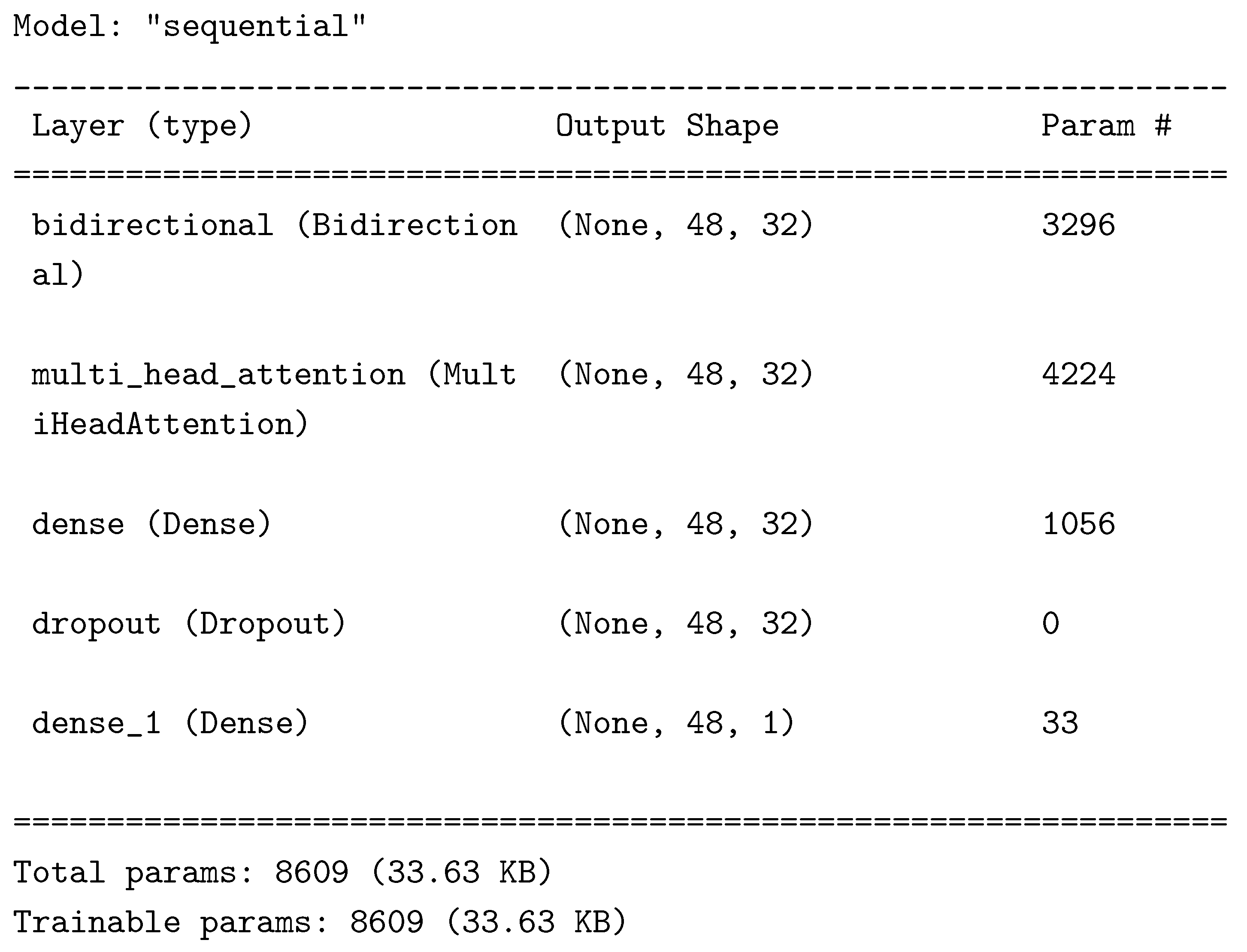
The data collected was sorted in different comma separated values files. The saved data was loaded through Python 3.9, preprocessed by filtering the quantile 0.8 of the frequency domain of the signal . The 8 signals were aggregated from 1 second to 1 hour granularity using their median values. Eventually the 8 signals were merged with the Temperature data for model (1) and with Humidity data for model (2), both at 1 hour granularity. Then the min-max scaler was fitted to transform each file separately. The ML algorithm selected for the data analysis is the Long Short-Term Memory (LSTM) Recurrent Neural Network [14] with peephole augmentation [15], wrapped by a Bidirectional layer. The LSTM requires 3 dimension as the input shape, with number of samples, number of observations (number of sequences) and number of features (number of voltage readings), we rearranged the data with a window of 48 hours, so to be able to identify circadian cycles of the temperature for each batch of data. We used the same approach to predict relative humidity in the air. Therefore, with N datapoints of voltage readings, we obtained a train shape of (N-48, 48, 8), while the validation size has been the floor of 0.2 times N-48. The files that did not have at least 48 datapoints as the validation dataset first dimension were discarded. The final shapes are (321, 48, 8) for the validation data and (321, 48) for the validation target, while (984, 48, 8) for the training data and (984, 48) for the training target.The ML problems defined (1) and (2) attempt to predict the (1) temperature and (2) humidity for the current hour (t) given 48 hours of previous data from time t-1 to time t-48. Through different trials we identified the following architecture for the Tensorflow layers.
The problem was implemented as a regression and the loss used was the mean squared error. The training was performed by minimizing the validation loss (the loss of the validation dataset) and also the coefficient was collected. The learning rate policy was starting at 0.00005 and increasing to reach 0.01 in the last epoch. The number of epochs was set to a maximum of 1200 and an early stopping criterion was defined which restored the model’s weights to those of the best performing iteration occurred. For a more detailed description see the CombinedLRScheduler class in the codebase 1.
3. Results
Both model (1) and (2) were assessed with validation data. The loss (Mean Squared Error) the model minimized is relative to normalized values ranging from 1 to 0. The Pearson and Spearman correlations are 0.72 and 0.66 for humidity and 0.78 and 0.7 for temperature. The Pearson and Spearman p-values are respectively 7.33 e-59 and 7.08 e-53 for the temperature, while 3.22e-41 and 1.69e-33 for the humidity. The Mean Absolute Error is computed eventually on the validation dataset with non-standardised values, to provide to the reader a more immediate understanding on the magnitude of the error. The predictions, hereby shown, were produced with time-continuous validation data originating from 3 of the 11 comma-separated files used (the remaining did not have sufficient contiguous observation to append to the validation dataset). The first chunk is relative to data from 08 June of 2023 to 09 June of 2023. In Figure 7, model (1) predictions were plotted in blue, against the observed temperature data in orange.
In Figure 8, model (2) predictions were plotted in blue, against the observed air humidity data in orange.
The second chunk is taken from 08 July of 2023 to 09 July of 2023. Model (1) produced the results depicted in Figure 9, featuring the following prediction (blue) for the observed temperature data (orange).
For the same dates, model (2) produced the results depicted in Figure 10, featuring the following prediction (blue) for the observed relative air humidity data (orange).
The third chunk is taken from 14 July of 2023 to 15 July of 2023. Model (1) produced the results depicted in Figure 11, featuring the following prediction (blue) for the observed temperature data (orange)
For the same dates, model (2) produced the results depicted in Figure 12, featuring the following prediction (blue) for the observed relative air humidity data (orange)
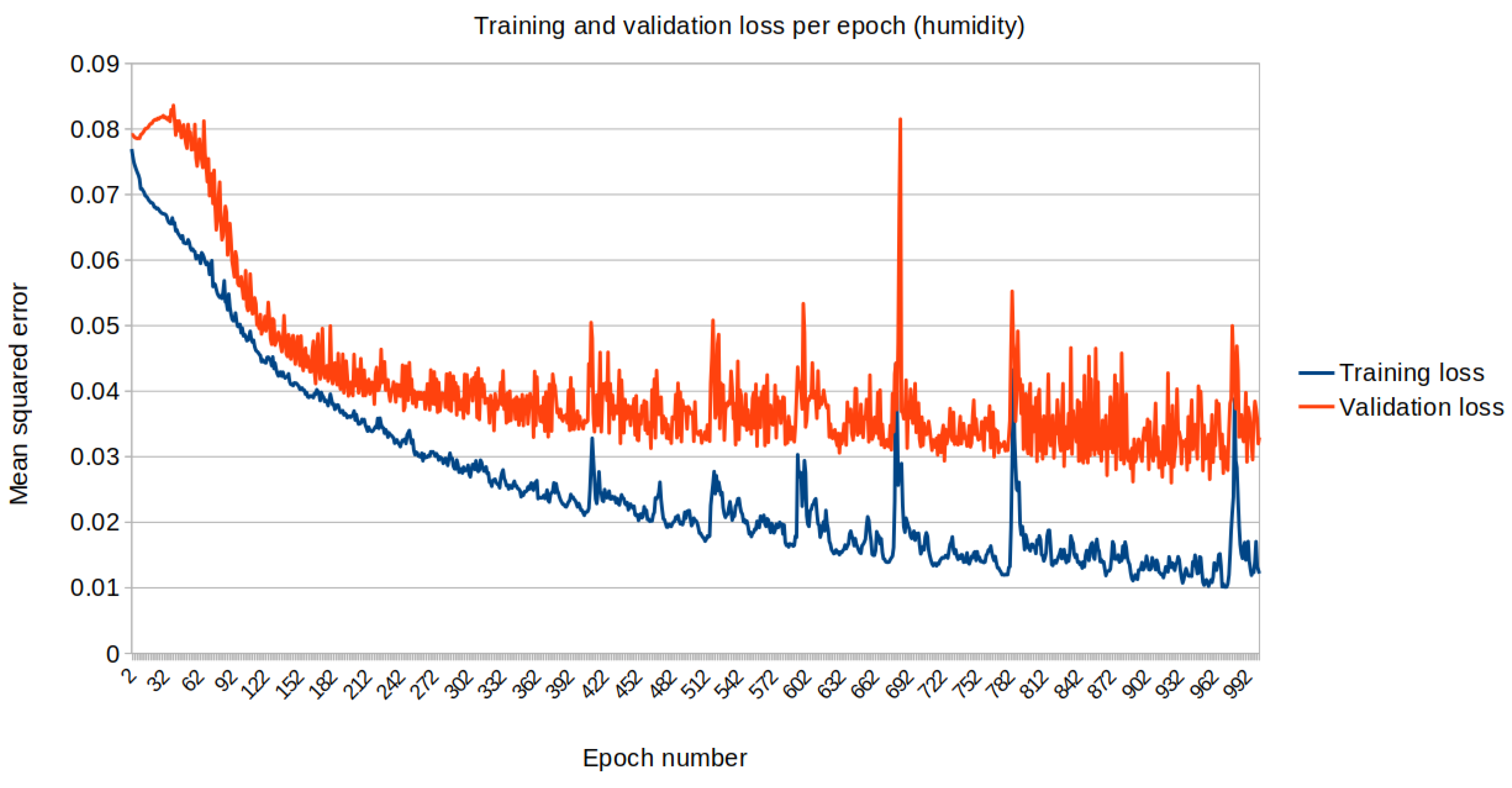
The mean squared error (loss) relative to the standardised data is eventually plotted along each iteration on the training dataset. Figure 13 and Figure 14 represent the loss for temperature and humidity standardised data respectively.
The mean has been computed of the mean absolute errors (MAEs) computed on the same non-standardised data of the validation dataset (originating from all the 11 files used). The average MAE obtained on the validation data is around 1.66 °C for the temperature and 7.35 % for the humidity. As a comparison, the typical accuracy for sensor-based (data assimilation) short-term weather forecasting and nowcasting is typically around 1-2 °C for temperature [16] and around 5-10% for humidity. [17]
4. Conclusions and Future Prospects
This study demonstrates the feasibility of using bioelectrical signals from Vitis vinifera as a rich, biologically grounded source of environmental information. By employing a robust data acquisition system and applying advanced machine learning models, we successfully predicted short-term meteorological parameters such as temperature and relative humidity with promising accuracy. The electrophysiological signals not only reflected the plant’s health status but also contained time-sensitive patterns aligned with rapid weather transitions, suggesting an innate environmental encoding within plant biopotentials.
Our findings support the concept that plants act as living sensors, exhibiting sensitivity to microclimatic fluctuations that can be computationally decoded. The high predictive performance of recurrent and attention-based models highlights the potential of biologically rooted weather forecasting systems, especially valuable in locations lacking dense sensor networks or in climate-sensitive agricultural regions.
Future work will focus on scaling up the study by incorporating a wider biodiversity of plant species and environmental conditions to generalize the models. Integration of multi-modal data (e.g., optical, thermal, chemical) alongside electrophysiology could enhance predictive granularity. Lastly, we envision the development of low-power, embedded hardware systems for real-time processing and edge inference, enabling the deployment of biohybrid weather stations. These advancements could revolutionize ultra-local environmental monitoring by fusing biological intelligence with modern AI techniques.
Author Contributions
Conceptualisation, A.C.; methodology, ALL; software, F.T. and G.P.B.; validation, ALL; formal analysis, ALL; resources, A.C.; data creation, A.C.; writing—original draft preparation, A.C.; writing—review and editing, ALL; visualisation, ALL; supervision, A.C. All authors have read and agreed to the published version of the manuscript.
Funding
Funding of the activities was granted by Zenit Arti Audiovisive, Torino, Italy, within the project: "Il codice del bosco". Furthermore we acknowledge proposal "DIVINO" (DIgital monitoring of VItis viNifera in vivO), selected for funding under the "NODES" (Nord Ovest Digitale E Sostenibile) Interreg National Funding cascaded calls, Next Generation EU, 2025.
Institutional Review Board Statement
Not applicable.
Data Availability Statement
Data will be made publicly accessible via Dryad
Conflicts of Interest
The authors declare no conflict of interest.
References
- Chaudhary, S.; Bajaj, S.B.; Mongia, S. Analysis of a Novel Integrated Machine Learning Model for Yield and Weather Prediction: Punjab Versus Maharashtra. In: Singh, Y., Verma, C., Zoltán, I., Chhabra, J.K., Singh, P.K. (eds) Proceedings of International Conference on Recent Innovations in Computing. ICRIC 2022. Lecture Notes in Electrical Engineering 2023, 83-93.
- Covert, M.W.; Gillies, T.E.; Takamasa, K.; Agmon, E. A forecast for large-scale, predictive biology: Lessons from meteorology. Cell Systems 2021, 12, 488–496. [Google Scholar] [CrossRef] [PubMed]
- Chiolerio, A.; Gagliano, M.; Pilia, S.; Pilia, P.; Vitiello, G.; Dehshibi, M.; Adamatzky, A. Bioelectrical synchronization of Picea abies during a solar eclipse. Royal Society Open Science 2025, 12, 241786. [Google Scholar] [CrossRef] [PubMed]
- Randriamandimbisoa, M.V.; Nany Razafindralambo, N.A.M.; Fakra, D.; Ravoajanahary, D.A.; Gatina, J.C.; Jaffrezic-Renault, N. Electrical response of plants to environmental stimuli: A short review and perspectives for meteorological applications. Sensors International 2020, 1, 100053. [Google Scholar] [CrossRef]
- de Toledo, G.R.A.; Parise, A.G.; Simmi, F.Z.; Costa, A.V.L.; Senko, L.G.S.; Debono, M.-W.; Souza, G.M. Plant electrome: the electrical dimension of plant life. Theoretical and Experimental Plant Physiology 2019, 31, 21–46. [Google Scholar] [CrossRef]
- Tran, D.; Dutoit, F.; Najdenovska, E.; Wallbridge, N.; Plummer, C.; Mazza, M.; Raileanu, L.E.; Camps, C. Electrophysiological assessment of plant status outside a Faraday cage using supervised machine learning. Scientific Reports 2019, 9, 17073. [Google Scholar] [CrossRef] [PubMed]
- Najdenovska, E.; Dutoit, F.; Tran, D.; Rochat, A.; Vu, B.; Mazza, M.; Camps, C.; Plummer, C.; Wallbridge, N.; Raileanu, L. E. Identifying General Stress in Commercial Tomatoes Based on Machine Learning Applied to Plant Electrophysiology. Applied Sciences 2021, 11, 5640. [Google Scholar] [CrossRef]
- Kozlova, E.; Yudina, L.; Sukhova, E.; Sukhov, V. Analysis of Electrome as a Tool for Plant Monitoring: Progress and Perspectives. Plants 2025, 14, 1500. [Google Scholar] [CrossRef] [PubMed]
- Imam, T.; Hasri, A.; Hidetaka, N.; Rofiq, A.R.; Ades, T. Deep learning algorithm for room temperature detection using bioelectric potential of plant data. Biomedical Signal Processing and Control 2025, 101, 107214. [Google Scholar]
- Cattani, A.; de Riedmatten, L.; Roulet, J.; Smit-Sadki, T.; Alfonso, E.; Kurenda, A.; Graeff, M.; Remolif, E.; Rienth, M. Water status assessment in grapevines using plant electrophysiology. OENO One 2024, 58, 8209. [Google Scholar] [CrossRef]
- Pereira, D.R.; Papa, J.P.; Rosalin Saraiva, G.F.; Souza, G.M. Automatic classification of plant electrophysiological responses to environmental stimuli using machine learning and interval arithmetic. Computers and Electronics in Agriculture 2018, 145, 35–42. [Google Scholar] [CrossRef]
- Rizzoli, A.; Jelmini, L.; Pezzatti, G.B.; Jermini, M.; Schumpp, O.; Debonneville, C.; Marcolin, E.; Krebs, P.; Conedera, M. Impact of the “Flavescence Dorée” Phytoplasma on Xylem Growth and Anatomical Characteristics in Trunks of ‘Chardonnay’ Grapevines (Vitis vinifera). Biology 2022, 11, 978. [Google Scholar] [CrossRef] [PubMed]
- Kalman, R.E. New Approach to Linear Filtering and Prediction Problems. Transactions of the ASME–Journal of Basic Engineering 1960, 82, 35–45. [Google Scholar] [CrossRef]
- Hochreiter, S.; Schmidhuber, J. Long short-term memory. Neural computation 1997, 9, 1735–1780. [Google Scholar] [CrossRef] [PubMed]
- Gers, F.A.; Schmidhuber, J. Recurrent nets that time and count. Proceedings of the IEEE-INNS-ENNS International Joint Conference on Neural Networks. IJCNN 2000. Neural Computing: New Challenges and Perspectives for the New Millenniu 2000, 3, 2. [Google Scholar]
- Openweather https://openweather.co.uk/accuracy-and-quality.
- Aguila, S.F. , Fuentes Barrios A.; Lorenzo S.L. Evaluation of the Nowcasting and very Short-Range Prediction System of the National Meteorological Service of Cuba. Environ. Sci. Proc. 2021, 8, 36. [Google Scholar]
| 1 |
Figure 1.
Left. Measurement setup showing the traditional vineyard where Vitis vinifera plants were connected to the biopotential acquisition device (battery-powered, protected by the orange waterproof cover). Double-shielded high fidelity cables are also shown running across the row. The setup was located in Cantina Adorno, Vigliano d’Asti (Monferrato, Italy). In the top inset, the ideal electrical connection scheme is shown, where two out of eight positive and negative leads and their related probes, series resistances () and series capacitances (), and measurement channel () are shown. Top right: connection scheme where plants connected are identified using capital letters, rows are indicated by the light blue lines, the data logger measurement device is at the center of the red disks, cables are identified by black arrows with their length reported in cm. Bottom right: distance and correlation scheme where plants are identified using capital letters, their distance and the inter-row distance in cm are evidenced by arrows, and a colour code is adopted on the basis of the correlation results (black: correlation , orange: positive correlation , light blue: negative correlation , red: positive correlation .
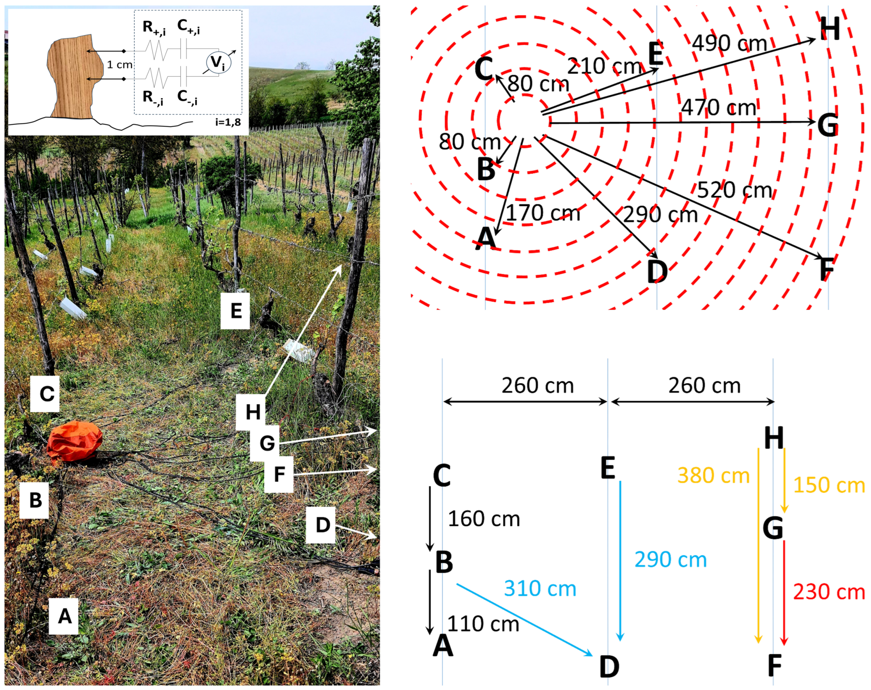
Figure 2.
Biopotential recordings taken from eight different individuals of Vitis vinifera (coloured curves from A to H) and a control chunk (black curve I), over a time lapse of 1000 seconds (16 mins 40 s) randomly selected within the entire dataset.
Figure 2.
Biopotential recordings taken from eight different individuals of Vitis vinifera (coloured curves from A to H) and a control chunk (black curve I), over a time lapse of 1000 seconds (16 mins 40 s) randomly selected within the entire dataset.
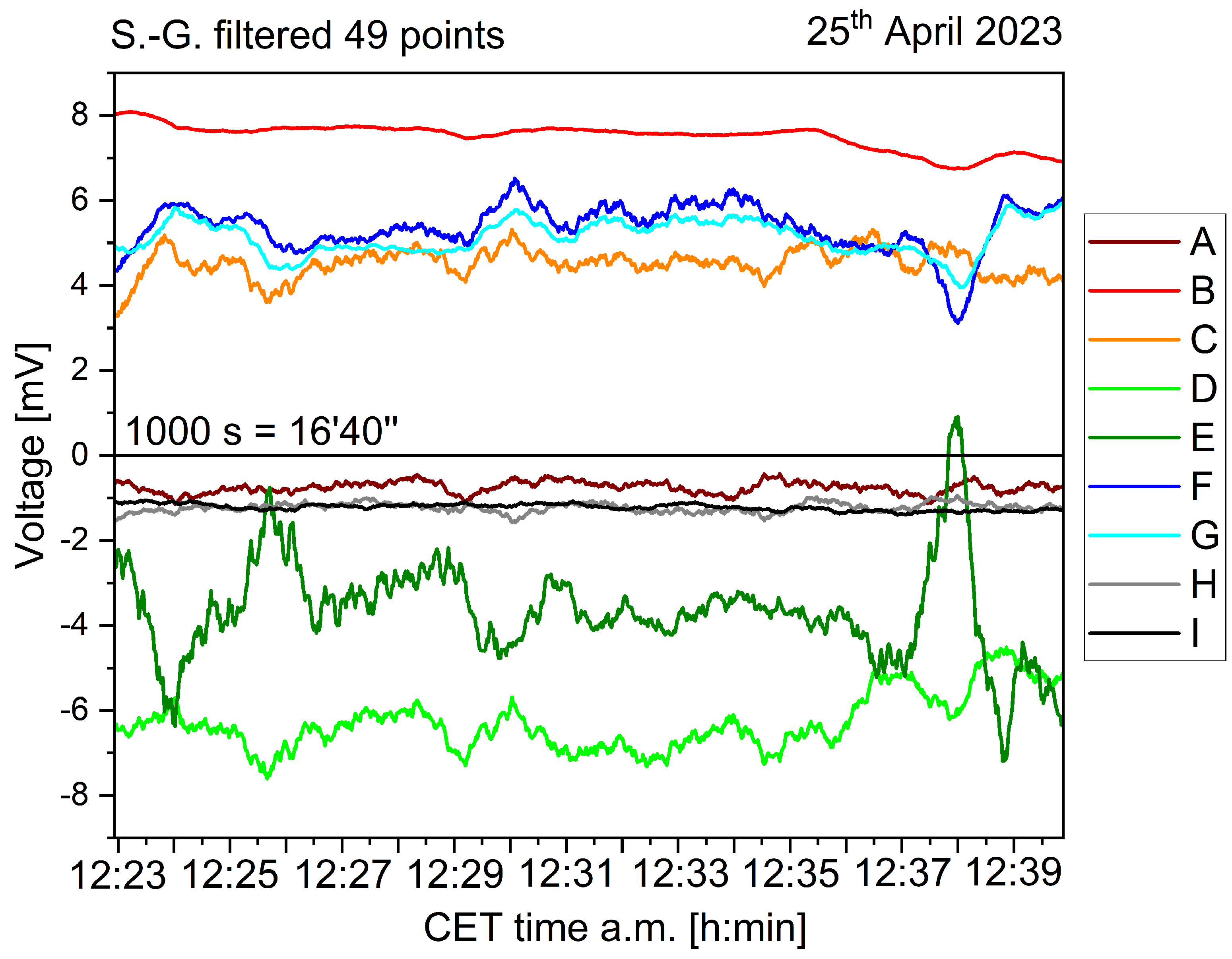
Figure 3.
Statistical features of Vitis vinifera biopotentials recordings (coloured curves from A to H) and a control chunk (black curve I), over a time lapse of 242 hours. Hystograms showing distributions with respect to a zero potential (all values expressed in mV).
Figure 3.
Statistical features of Vitis vinifera biopotentials recordings (coloured curves from A to H) and a control chunk (black curve I), over a time lapse of 242 hours. Hystograms showing distributions with respect to a zero potential (all values expressed in mV).
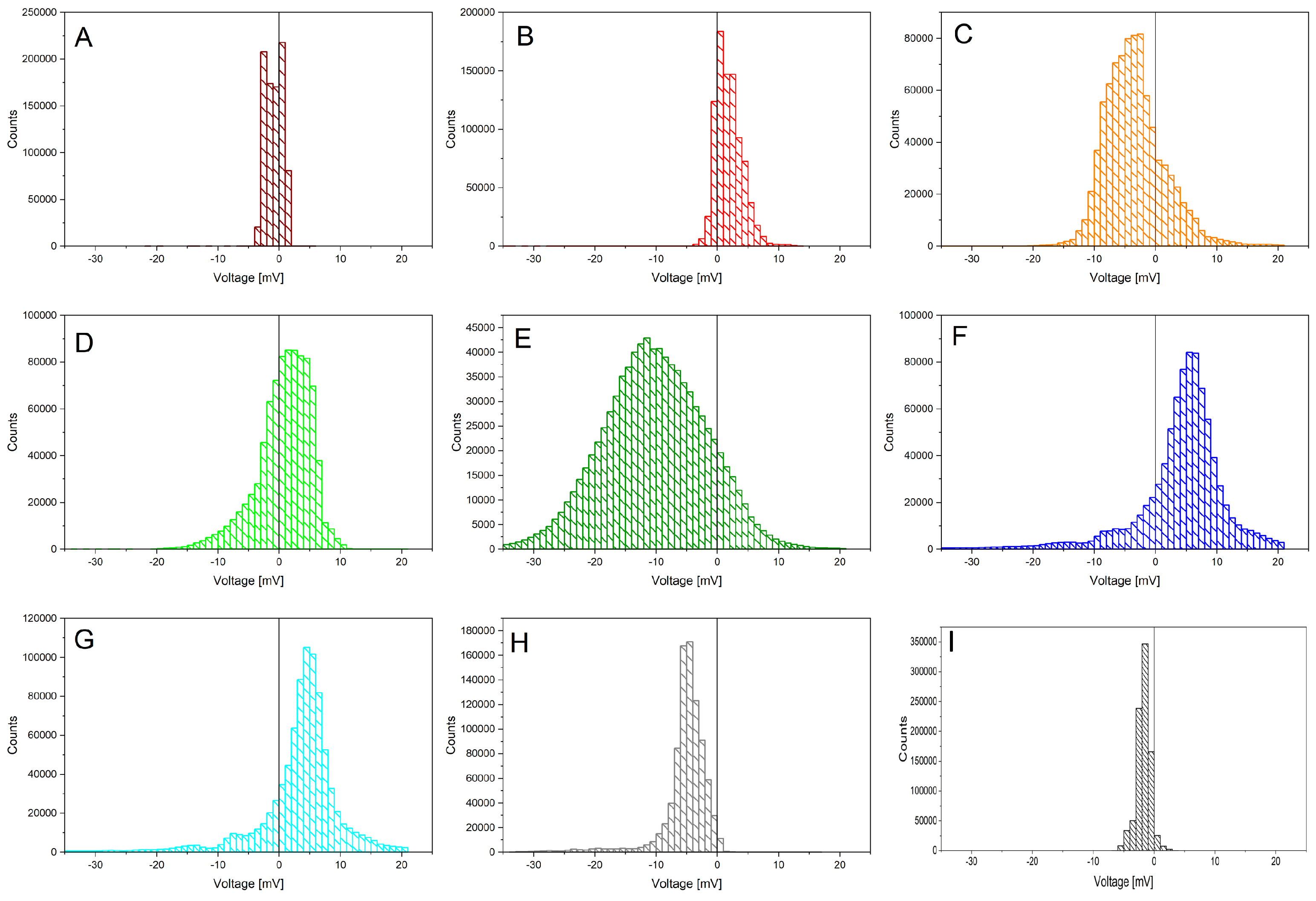
Figure 4.
Statistical features of Vitis vinifera biopotentials recordings (coloured curves from A to H) and a control chunk (black curve I), over a time lapse of 242 hours. Boxplot showing for each process its outliers (full rhomboids), its interquartile population (filled rectangles), the extended interquartile range corresponding to 150 % span of the previous quantity (limited segment), the median (horizontal segment), and mean (open square).
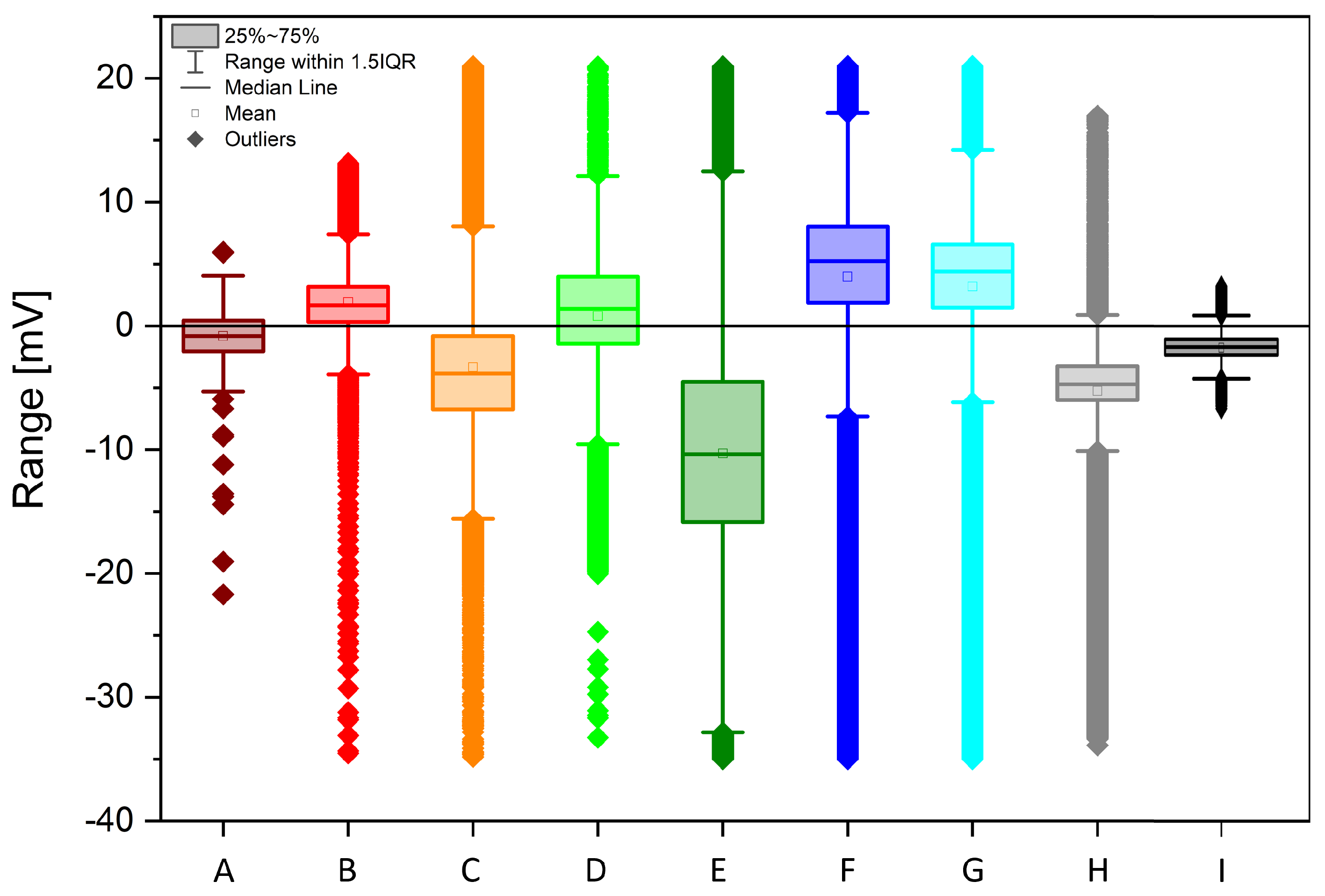
Figure 5.
Statistical features of Vitis vinifera biopotentials recordings, over a time lapse of 242 hours. From top to bottom, from left to right: heatmap showing Pearson’s correlation coefficients, related p-values, Spearman’s correlations coefficients, related p-values.
Figure 5.
Statistical features of Vitis vinifera biopotentials recordings, over a time lapse of 242 hours. From top to bottom, from left to right: heatmap showing Pearson’s correlation coefficients, related p-values, Spearman’s correlations coefficients, related p-values.

Figure 6.
Fast Fourier Transform (FFT) analysis of the dataset, comparing the different sites from "A" to "H" and the cut log of a vine "I". Data shows the logarithm of the Time-Integral Squared Amplitude (TISA) versus the logarithm of the frequency, filtered applying a Savitzki-Golay first order function over 199 experimental points.
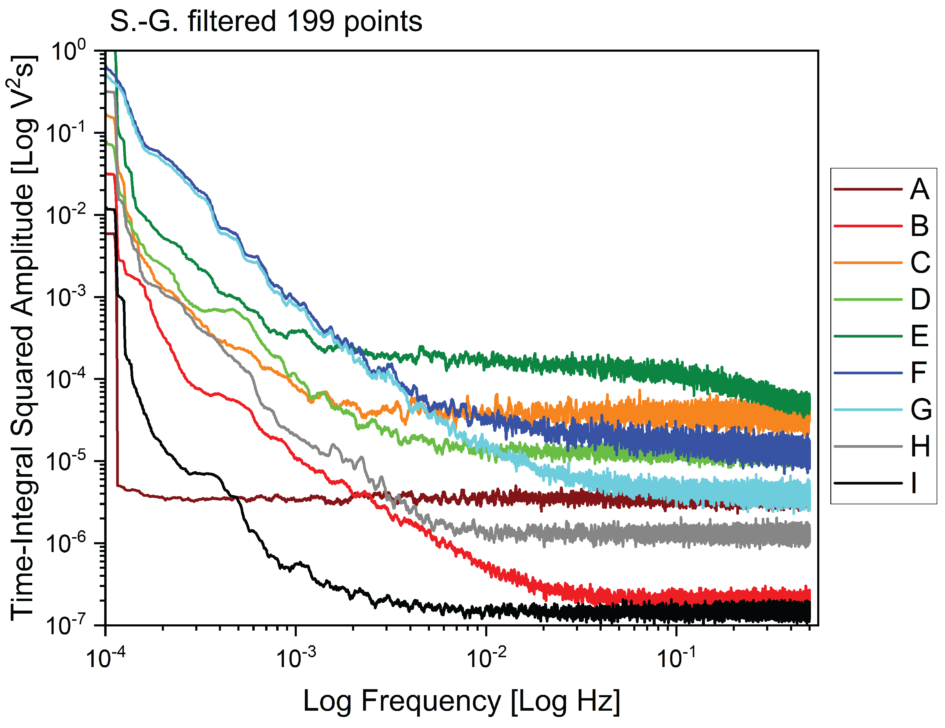
Figure 7.
Predicted (blue) vs Observed (orange) temperature.
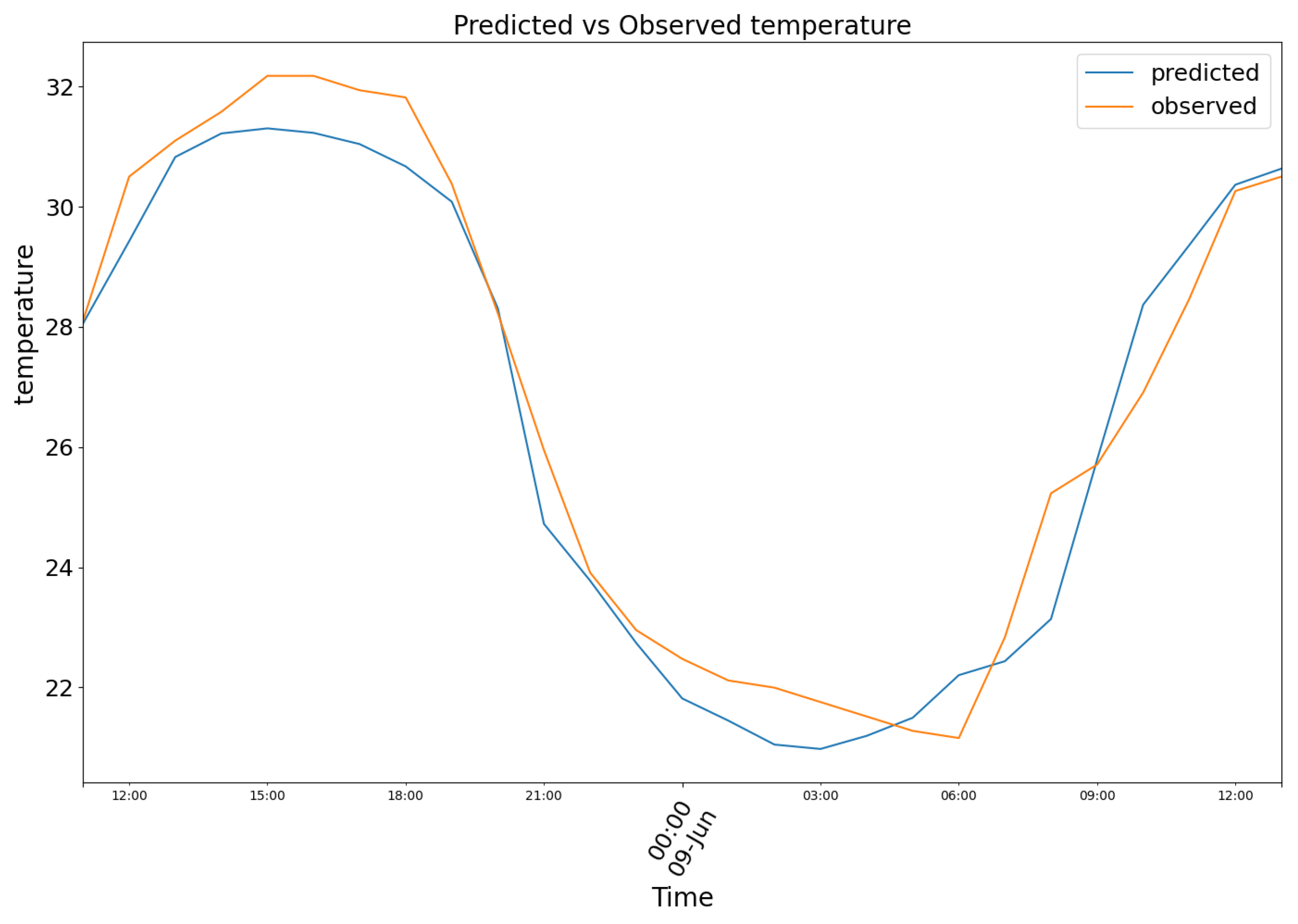
Figure 8.
Predicted (blue) vs Observed (orange) humidity.
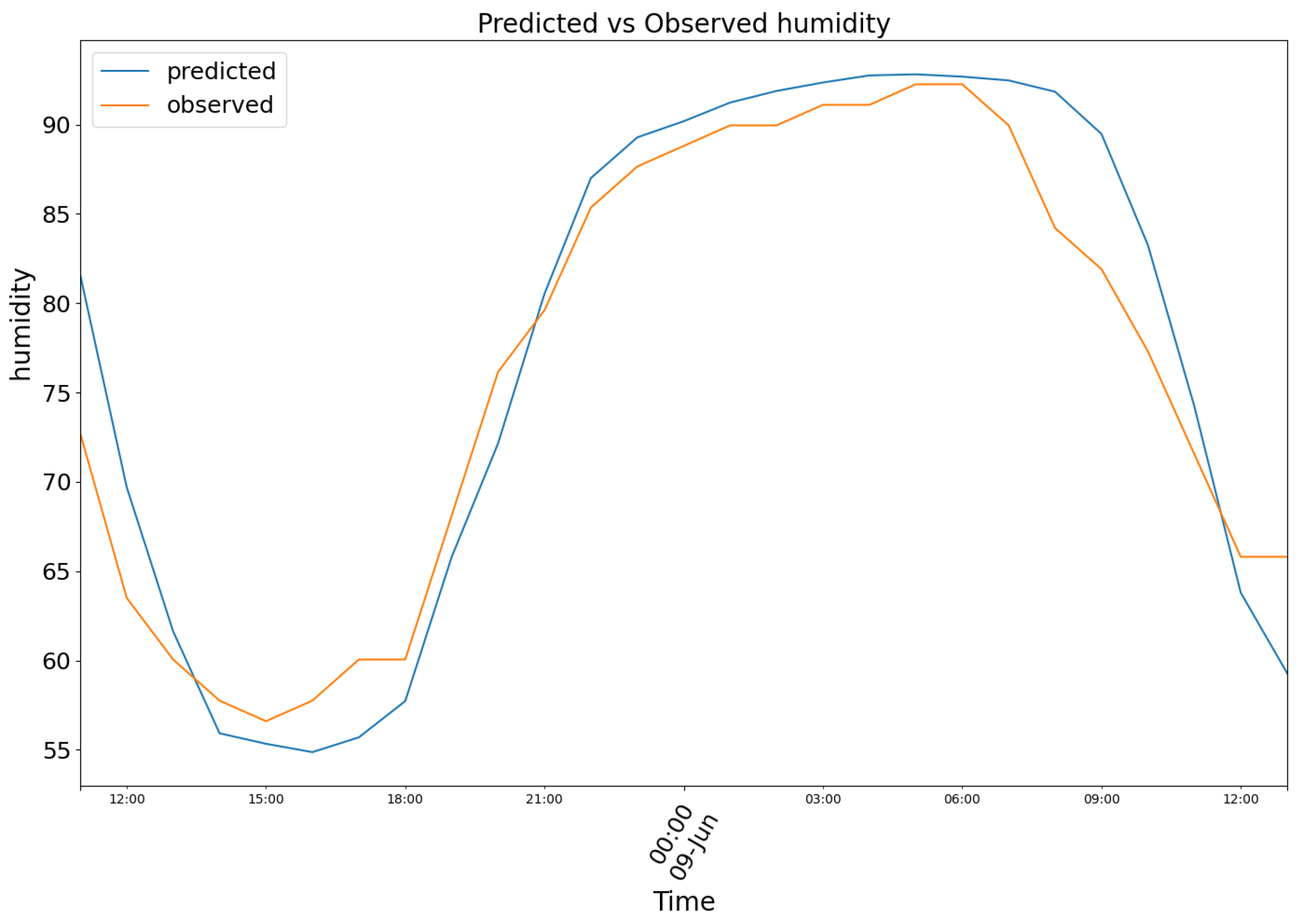
Figure 9.
Predicted (blue) vs Observed (orange) temperature.
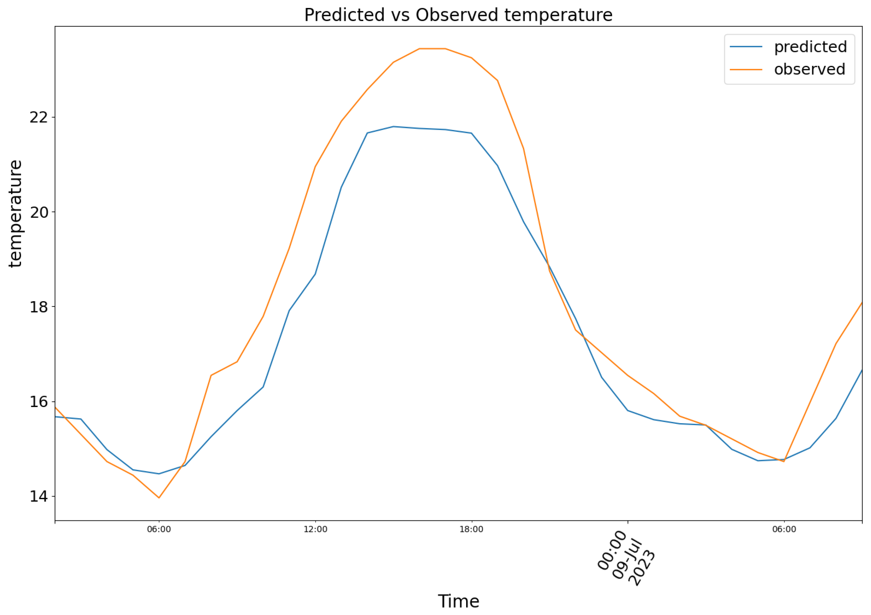
Figure 10.
Predicted (blue) vs Observed (orange) humidity.
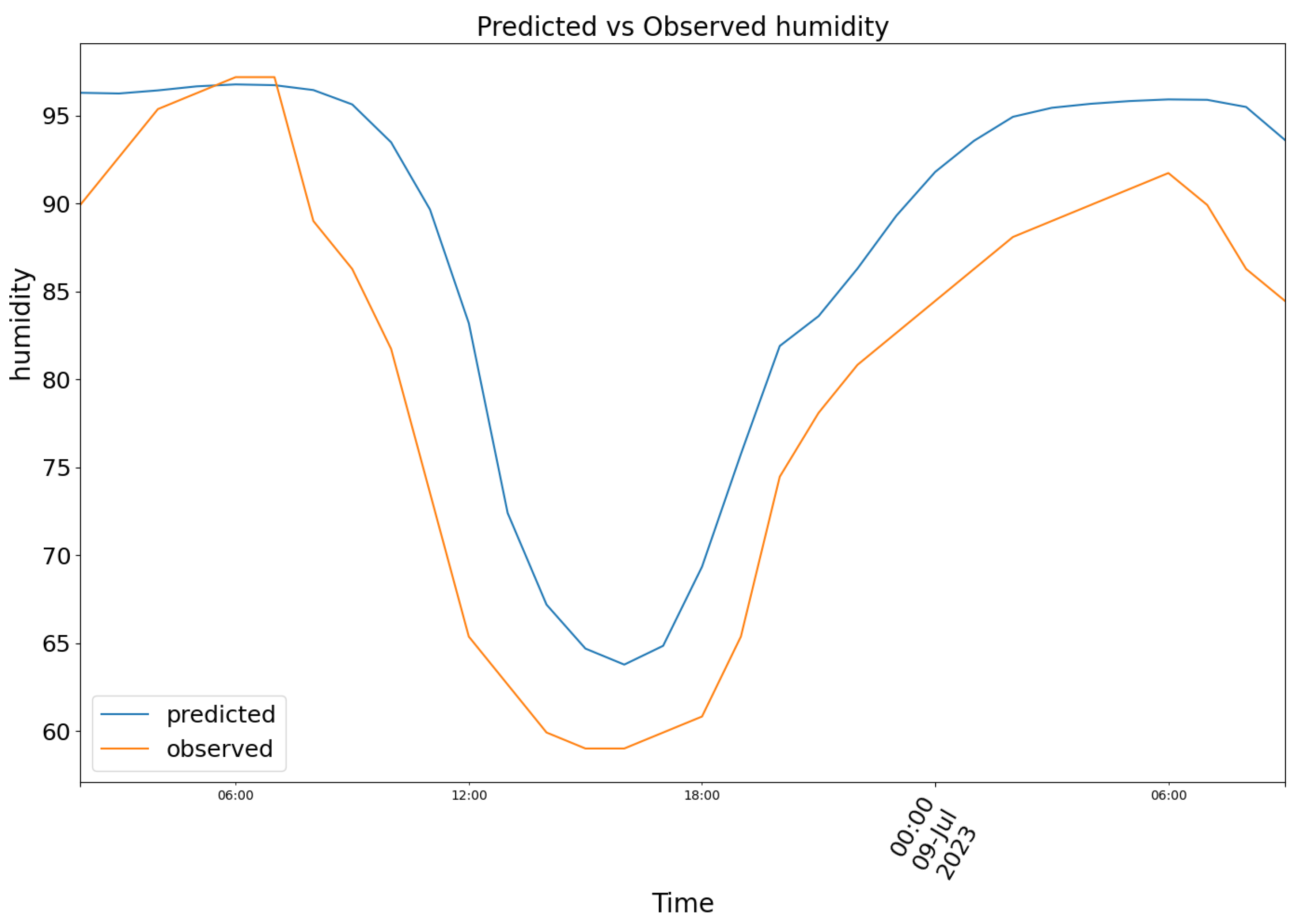
Figure 11.
Predicted (blue) vs Observed (orange) temperature.
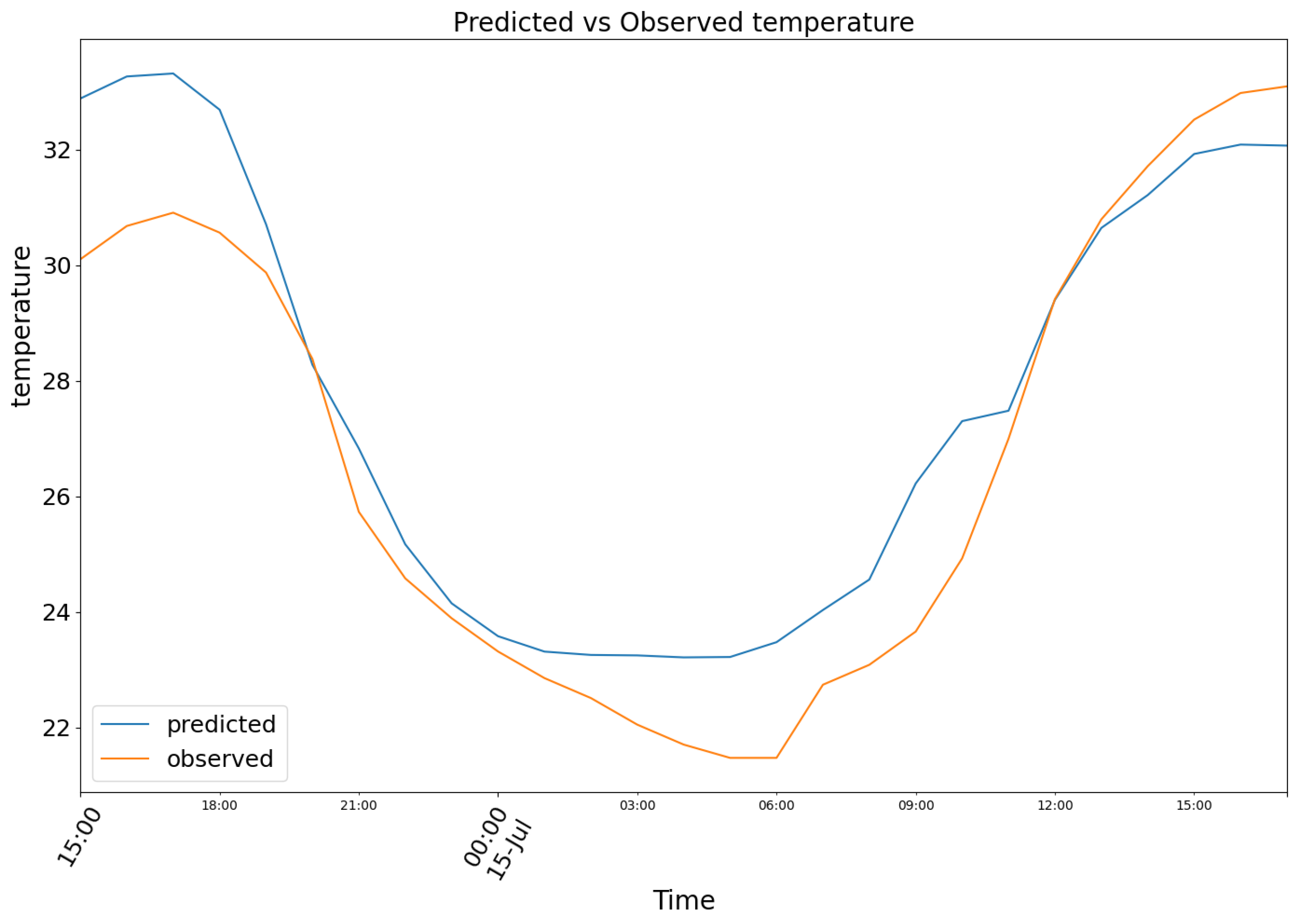
Figure 12.
Predicted (blue) vs Observed (orange) humidity.
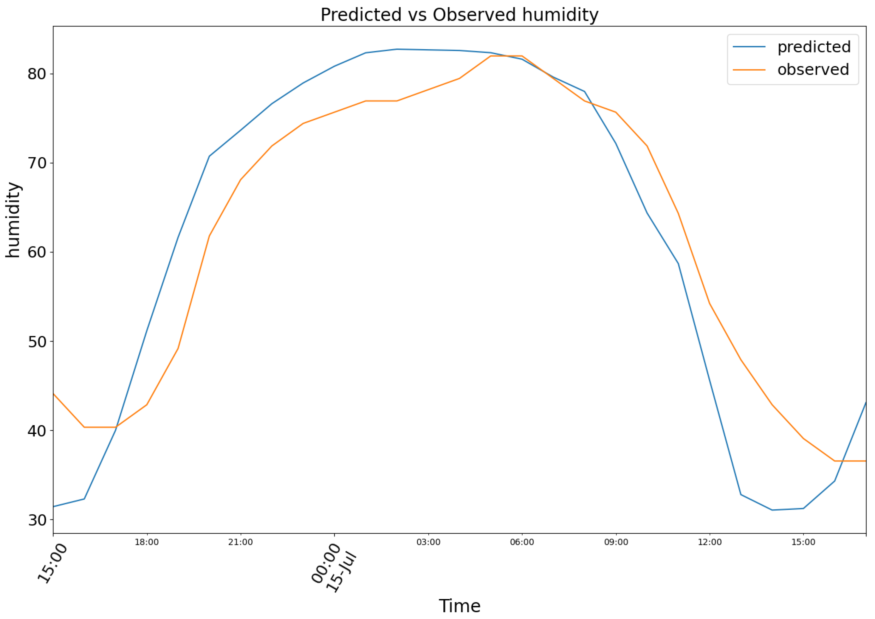
Figure 13.
Training (blue) vs Validation (orange) dataset loss for temperature.
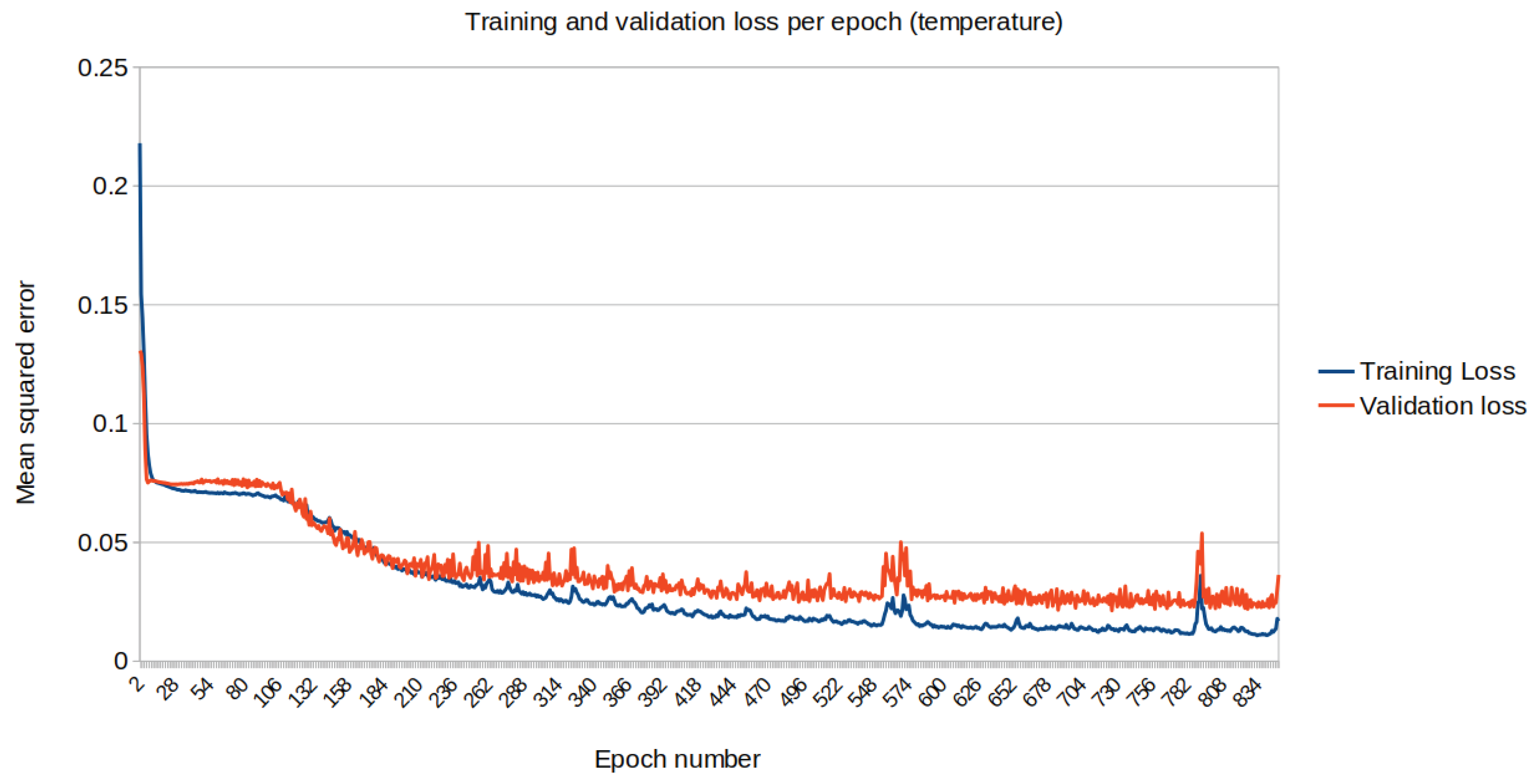
Figure 14.
Training (blue) vs Validation (orange) dataset loss for air humidity.
Disclaimer/Publisher’s Note: The statements, opinions and data contained in all publications are solely those of the individual author(s) and contributor(s) and not of MDPI and/or the editor(s). MDPI and/or the editor(s) disclaim responsibility for any injury to people or property resulting from any ideas, methods, instructions or products referred to in the content. |
© 2025 by the authors. Licensee MDPI, Basel, Switzerland. This article is an open access article distributed under the terms and conditions of the Creative Commons Attribution (CC BY) license (http://creativecommons.org/licenses/by/4.0/).
Copyright: This open access article is published under a Creative Commons CC BY 4.0 license, which permit the free download, distribution, and reuse, provided that the author and preprint are cited in any reuse.


