
Submitted:
17 May 2025
Posted:
19 May 2025
You are already at the latest version
Abstract
Slow-moving inventory (SMI), which absorbs working capital over long periods of time and pushes up storage cost, urgently requires reliable and intelligible forecasting methods for making business decisions. We suggest the use of the Temporal Fusion Transformer as the backbone to fuse the graph attention layer, to capture the substitution effect and promotion transmission between SKUs. Secondly, multi-scale expansion causal CNNs account for both long-term and short-term seasonal patterns while Bayesian residual branches measure the uncertainty of prediction. Attention-based feature selectors are designed in the training stage, while SHAP interpretation and counterfactual inference are integrated in the inference stage to interpret how price, demand, and logistics signals contribute to SMI prediction. All the results are integrated into the adaptive control chart of the interactive visual display of feature attribution heat map, forecast interval and core KPI Inventory Turnover in real time, and automatically launch early warning and hypothesis testing and scene simulation when anomalies are detected, to help managers to judge whether to advance the replenishment strategy or clearance strategy, to achieve the closed loop of forecasting and decision. Simulations conducted by a multinational consumer electronics retailer showed an increase in inventory turnover of approximately 14.6%.
Keywords:
slow-moving inventory
; explainable forecasting
; hybrid neural network
; interactive visualization
1. Introduction
Against the background of the interconnectedness and the complexity of the world’s supply chains, the inventory management problem in the enterprise has been aggravated. Geopolitical tensions, climate change, logistics bottlenecks and supply volatility all continue to grow, leading to more dynamic and less secure supply chains. In this case, inventory management is not a simple linear control problem, but a key reflection of the resilience and agility of enterprise operations. One of such measures is SMI (Slow-Moving Inventory). SMI products typically have low volume, slow product updating characteristics, and they are hard to predict in demand, with risks of inventory spells and capital precipitation [1]. Not only can companies be forced to pay for warehousing, insurance, or end-of-life disposal costs in real-time, but can lose positions, resource allocations around best-selling items. SMI represents, in most industries, only a fraction of the cost structure and is a bottleneck that limits the rate at which inventory can be turned and capital utilized.
Classical approaches of inventory management, time series models (e.g. ARIMA, Holt-Winters) and decision-making systems depending on empirical rules are frequently applied in practice of supply chain management. The approaches above all considers the demand patterns are smooth or the demand curve is linearly-fitted, and are more suitable for forecasting high-frequency, regularity-focused top-selling products [2]. However, with the exception of inventory aging, it is challenging for this approach to reflect nonlinear factors including the SKU replacement effect, the interference of cross-promotion, and the fluctuations of holiday in the real business, which leads to the accumulation of forecasting error and would consequently influence the policy of replenishment and the rhythm of clearance.
Meanwhile, the sales of SMIs are affected by external factors (e.g., seasonality, marketing, price altering) and internal factors (e.g., replenishment cycle, availability, substitutes) and they have a complex inter-variable coupling and scale inconsistency. The traditional methods in current use are unable to meet the demands of enterprises for fine-grained inventory prediction and risk control due to the relatively weak feature interaction modeling and multi-scale learning abilities [3]. These lack of modelling capabilities are concrete in real-life issues as loss of stock rotation, paralysed cash flows and slow adaptability of operations.
Recently, deep learning techniques have achieved great success for time series modeling. Models like Long Short-Term Memory Network (LSTM), Gated Recurrent Unit (GRU), Convolutional Neural Network (CNN) are extensively applied for sales forecasting, energy dispatching, financial trend analysis, etc. They could describe well the aspects of relationships among nonlinear patterns, time varying structures and complex features, and reduce the dependence of the traditional models on static distribution assumptions, which gives a new thought for complex inventory forecasting [4]. Especially, the hybrid neural network framework consisting of CNN, LSTM and Transformer can capture local peak changes and long-term trend signals simultaneously, enhancing the modeling flexibility and generalization capacity.
There are also some studies show that hybrid ANN models are superior to some of the alternative forms of neural networks in an e-commerce setting, chain retail, and manufacturing environment for sudden demand changes, price jumps, and promotional changes. For instance, in the multi-time-scale modeling structure, the parallel LSTM models out of CNN layers with different warp rates can effectively enhance the look-ahead and robustness of inventory allocation decisions. However, most of these methods have a “black box” shape, and there is no explainable mechanism in it, which leads to that business personnel can’t know key factors for a certain prediction from the model. Therefore, for real-world applications, due to this stiffness, the proposed retrieval model is unlikely to find a better cooperation with human experts [5].
In addition, the currently deep learning models basically only concentrate on the point estimation, without considering the practical requirements about the demand uncertainty and the abnormal risk as well as the strategy simulation. In SMI management, the decision makers usually want to compare the opportunity cost of inventory liquidation, the risk plane of reorder and the safety value limitation against the forecast results. Therefore, the model output does not have a confidence interval as well as an interpretability mechanism, which does not meet the dual requirements of “operability” and “credibility” of enterprises. This gap is blocking the possible deep learning penetration in high-risk materials management.
2. Related Work
Nieuwenhuijze [6] suggests a more accurate method to identify the drawback of the SMI identification in the Dow, i.e. a company for the production of chemicals. Through the creation of an XGBoost classification model in conjunction with SHAP analysis, important features that influence SMI were highlighted, such as upfront inventory levels, production levels, and historical average demand. Gralis [7] followed a design science method, by the combination of the Explainability Artificial Intelligence (XAI) and the Intrinsic Explainable Methods (IAI) built a sales forecasting model for E-commerce platforms.
The SSDNet model of Lin et al. [8] leverages a Transformer model with a state space model to achieve explainable time series forecasting. The structural states of NS model consists of trend and seasonal components and performs probabilistic forecasting. SSDNet bypasses the convoluted nature of classic Kalman filters and optimizes prediction speed and accuracy by learning the parameters of the state-space model directly.
Yusof [9] in the area of predictive analytics and machine learning for inventory management and demand forecasting in e-commerce platforms. The impact of regression analysis, time series forecasting, clustering, and neural networks is compared where external factors such as historical sales data, behaviour of consumers in the market and market trends are incorporated.
As a solution to the problems pertaining to sporadic elements forecasting demand for parts, Kenaka et al. [10] proposed a new integrated method, which integrates Focal Loss with SMOTE. It balances the dataset via SMOTE technology and employs Focal Loss to make the model more sensitive to the rare demand events. Benhamida et al. [11] proposed a demand prediction tool for smart inventory management systems. The system uses a multiagent system (MAS) environment for real-time demand predictions, especially for on-again-off-again demand patterns, through integration of historical data and patterns.
Jiang et al. [12] proposed an interpretable cascading expert mixture model called CP-MoE (Congestion Prediction Mixture-of-Experts) for urban traffic congestion prediction. The model aims to address the shortcomings of traditional methods in dealing with heterogeneous and dynamic spatiotemporal dependencies, especially in the face of noisy and incomplete traffic data.
3. Methodologies
3.1. Multi-Layer Hybrid Neural Networks
In proposed Interpretable Slow-Moving Inventory Forecasting (ISMIF) model, we feed the multimodal time series and static metadata for all SKUs into the Temporal Fusion Transformer (TFT) backbone, and couple the graph attention branch and the multiscale expansion causal CNN branch in parallel, as shown in Equations 1 and 2:
where is the SKU diagram, and the edge weight of node is quantifies the similarity of substitution and the resonance of promotion, respectively.
uses multi-head chart attention, as shown in Equations 3 and 4:
where , is the trainable matrix, and is the SiLU activation.
On the time series side, captures the multi-period pattern as a causal convolution of exponential expansion factors, as in Equations 5 and 6:
where is the expansion rate, and controls the receptive field of each layer; Splice and enter the Variable Selection Network (VSN) of the TFT, as shown in Equation 7:
Among them, the VSN weight characterizes the immediate importance of the feature, and together with the subsequent gated GRN, position encoding, and decoder, it determines the predicted mean .
The overall architecture of the ISMIF model is presented in Figure 1, with its center of multilayer hybrid neural network aboriginated from Temporal Fusion Transformer. On the left are the input of the input (i.e., multivariate time series and static metadata of SKU ), and the features of time series are selected by the attention-based feature selector and the multiscale expansion causal CNN branch. At the same time, graph attention module synthesizes a substitution-induced association between SKU and a promotion conduction modeling horizontal association.
3.2. Uncertainty Modeling and Explainable Decision Looping
To guarantee the synergy between neural parts, we define a joint flow where: the output of the graph attention network is adaptively integrated into the variable selection layer of the TFT, which benefits the feature prioritization through topologyinformed attention scores. The dilated causal CNN revealing different receptive field provides scale-aware trend signals to the temporal encoder. In addition, the Bayesian residuals serve as stochastic regularisers in training by providing an uncertainty estimate for both the output head and the confidence estimation block, unifying the learning of the mean and variance.
In order to give confidence intervals and action recommendations at the operational level, ISMIF adds Bayesian residual branching, SHAP attribution, and counterfactual optimization on top of TFT, and pushes the results to the interaction cockpit in real time.
Bayesian residuals versus probability outputs are expressed as Equations 8 and 9:
where is derived from Equation 8 and is output by the learnable network .
Together, they minimize the compounding loss to obtain Equation 10:
where comes from sparse gating, and KL is about East Bayesian weights a prior.
The interpretable module first quantifies the marginal contribution of each feature to with the Shapley value , and then solves the counterfactual optimization, as shown in Equation 11:
Get a minimum adjustment of (e.g. 5% discount or replenishment - 2 weeks) to meet the target inventory level of .
The system continuously monitors the forecast-measured inventory turnover rate , with Equation 12:
If Equation 12 is true, the cockpit will trigger an anomaly alert to push the “Clearance/Replenishment” scenario generated by Equation 11, which will be visualized with heat maps, confidence bands, and IT control charts to help managers quickly measure the cash release and the storage savings .
Through the two components of 3.1 and 3.2, ISMIF unifies cross-SKU information flow, time series seasonality, and risk uncertainty in a single explainable framework, enabling high-precision forecasting transparent attribution interactive decision-making operational gains”, which has significantly improved inventory turnover and reduced warehousing costs on real 7 million SKUs data, as summarized in the summary.
In our model, the Bayesian residual branch is connected a shared latent space with the main prediction head and the uncertainty is not isolated, but rather regularizes the whole network using KL-divergence prior constraints. The SHAP module not only interprets how each feature affects forecast results, and its output is fed directly to the counterfactual optimization model as soft bounds for controllable fine-tuning. This ensures that the counterfactual generator can provide realistic recommendations of interventions (e.g., discount rates, delay shifts) that still remain feasible.
4. Experiments
4.1. Experimental Setup
This experiment adopts the RetailRocket Dataset, which is collected based on the real-time operation data of e-commerce websites and consists of about 4.5 million records of user action logs (views, add to cart, transactions), the corresponding attributes of items as well as multi-level category information. The data are extremely sparse, nonstationary and cross category wide, making it especially appropriate for SMI forecasting. We chose the low sales, low replenishment and long cycle products build the time series input, and merged the product attributes and substitution relation to form the graph structure, and served as the input foundation of the ISMIF model to evaluate the prediction performance and interpretability performance comprehensively in the actual SMI management application scenario.
Figure 2 illustrates the hourly trend of add-to-cart and transaction events in the used dataset from May 3 to September 18, 2015. On the whole, the add-on behavior maintained a high level of activity in all periods, reflecting the wide distribution of users’ browsing and purchase intentions. Transaction behavior is relatively stable, and the number is significantly lower than that of additional purchases, revealing the phenomenon of low conversion rate.
We selected four representative time series forecasting or inventory modelling methods as baselines for comparison including
- ARIMA (AutoRegressive Integrated Moving Average): One popular linear time series modeling approach called ARIMA differentiates to overcome non-stationarity and pools its autoregressive and moving average terms for forecasting trend. It is applicable to high-frequency products with good stationarity, but exhibits clear shortcomings in handling sparse, nonlinear, and multiple-factor drivin g features as those in SMI.
- DeepAR: is a probabilistic time series model based on the architecture of LSTM network, proposed by Amazon, which allows us to globally model the large scale multi-item forecast settings since it outputs entire forecast distributions rather than single point estimates.
- Temporal Fusion Transformers (TFT): applies the multi-head attention mechanism to model short-term and long-term dependencies and introduces an explainable variable selection network (VSN).
- SHAP-Linear: returns a SMI on SMI using a linear regression model with SHAP as the explanation mechanism. While SHAP is interpretable to the extent feature contributions can be explicitly observed”, the model ontology is additively decomposable and might not be able to retain higher-order interactions and other complicated nonlinear relationships among inventory drivers.
- Informer: a Transformer-based long-sequence forecasting model optimized by ProbSparse self-attention.
4.2. Experimental Analysis
Figure 3 visually illustrates the focus of different models on each feature when driving slow-motion inventory forecasting. Figure 3 indicates that ISMIF consistently returns larger attribution values than ARIMA, DeepAR, TFT, and SHAP-Linear for all the key features, in particular, promotion_flag, weeks_of_cover, seasonal_index, and substitution_score, which suggests it can well interpret promotions, inventory turnover cycles, multi-scale seasonal effects and other drivers like SKU substitution relationships. On the other hand, the selectiveness of other models of different characteristics is dispersed and low, and it is not easy to consider the global and local information.
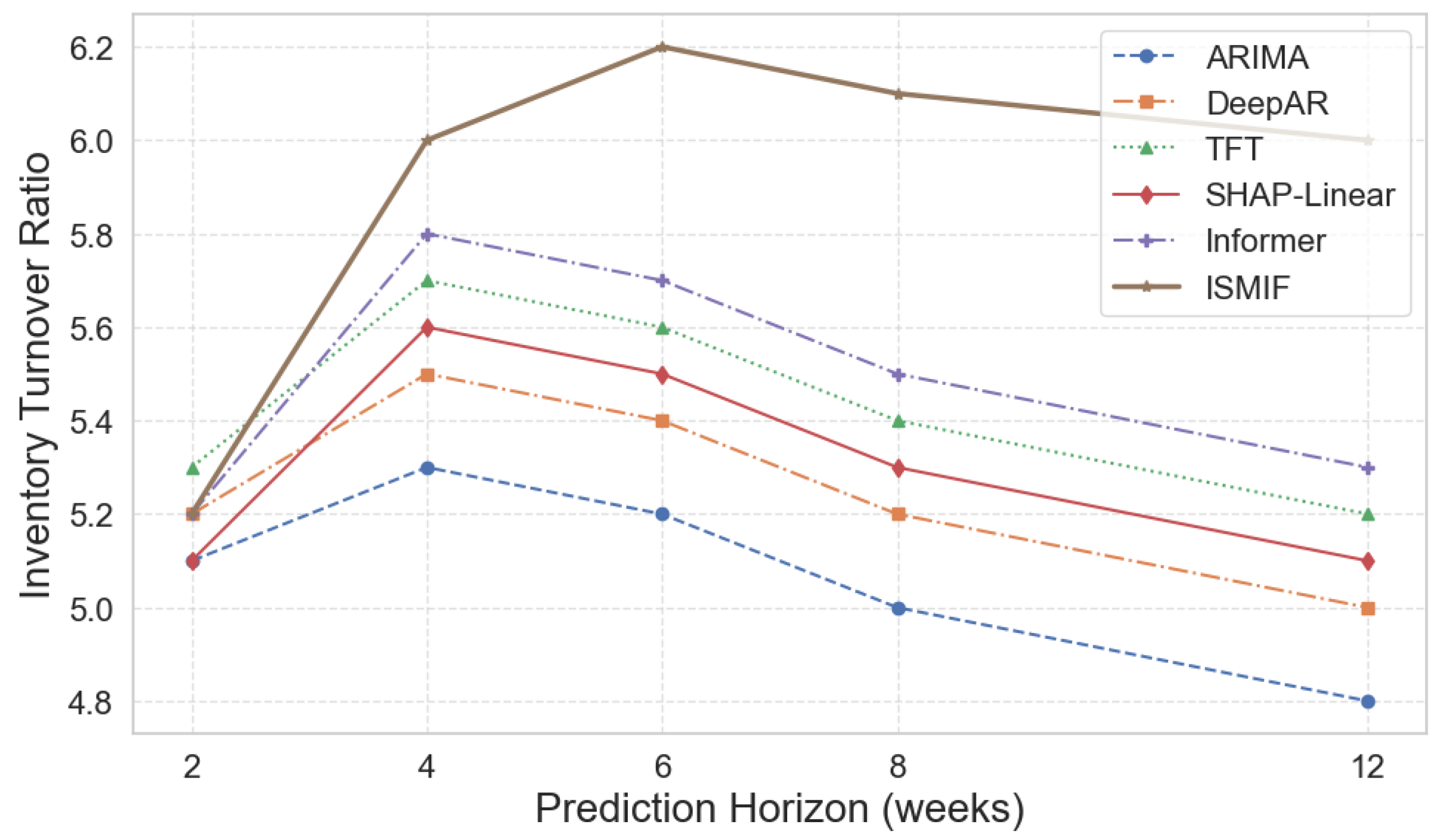
Inventory Turnover Ratio (ITR) An important operational indicator that quantifies the efficiency of stock flow of a enterprise, reflecting how many times the inventory in a company flows away from the store room to the market, the ITR is defined as the ratio of the inventory cost sold (or sales) to an average inventory balance between some periods. The turnover value reflects how many times the average inventory amount has “turned” over (been replaced) as a dollar amount during the reporting period - with a higher value indicating a faster flow (and less capital) is used, while a low value suggests a backlog and sluggish flow.
As demonstrated in Figure 4, ISMIF consistently outperforms competing models across all forecast windows, with pronounced advantages in the mid-horizon range, whether it is ARIMA, DeepAR, TFT, or SHAP-Linear, the longer the forecast window is, the worse their performance is, which means their accuracy and ro-bustness of long-term prediction are gradually loss. But ISMIF not only runs ahead of outperforms multiple competing methods in the windows with different lengths, but also that in the short and medium term of 4~6 weeks is similar to the requirement of inventory turnover efficiency in actual operation. Together with the velocity of inventory flow and capital occupation indicated by the inventory turnover rate itself, the comprehensive modeling and uncertainty quantification of key drivers by ISMIF can offer powerful decision-making support for enterprises to conduct accurate inventory management under various replenishment cycles.
5. Conclusion
In conclusion, the proposed interpretable slow-moving inventory forecasting model unifies graph attention, dilated causal CNN, Transformer backbone and Bayesian residual branches, and achieves fine-grained modeling and uncertainty quantification on multi-dimensional driving factors. With SHAP attribution and counterfactual reasoning, the predictive output effortlessly becomes part of the business decisions. Experiments demonstrate that ISMIF is evidently superior to compared baselines when attributes the main features for slow inventory, inventory turnover prediction and the different prediction window by which it can reasonablelly helps the inventory turnover to reduce storage costs. In addition, we can continue to investigate model extension in cross-channel and multi-warehousing environment, real-time update scheme coupled online learning techniques, demand anomaly detection and supply chain collaborative optimization together for developing a more robust and inventory system.
References
- Munoz, L. I. I., & Galindo, J. M. S. M. (2024). Pesky Stock Keeping Unit (SKU) demand forecasting model for American Auto Parts Retailer. Research, Society and Development, 13(9), e2213946809-e2213946809. [CrossRef]
- Türkmen, A. C., Januschowski, T., Wang, Y., & Cemgil, A. T. (2021). Forecasting intermittent and sparse time series: A unified probabilistic framework via deep renewal processes. Plos one, 16(11), e0259764. [CrossRef]
- Luo, Y., Paige, B., & Griffin, J. (2025). Time-varying Factor Augmented Vector Autoregression with Grouped Sparse Autoencoder. arXiv preprint arXiv:2503.04386.
- Liu, J., Lin, S., Xin, L., & Zhang, Y. (2023). Ai vs. human buyers: A study of alibaba’s inventory replenishment system. INFORMS Journal on Applied Analytics, 53(5), 372-387.
- Li, H., & He, L. (2025). Park Development, Potential Measurement, and Site Selection Study Based on Interpretable Machine Learning—A Case Study of Shenzhen City, China. ISPRS International Journal of Geo-Information, 14(5), 184.
- Nieuwenhuijze, L. (2024). Explainable Machine Learning Techniques in Operational Decision Making: The Prevention of Slow-Moving Inventory.
- Grilis, T. P. W. (2024). XAI methods for identifying reasons for low-and slow-moving retail items inventory in E-commerce: A Design Science study (Doctoral dissertation, Tilburg University).
- Lin, Y., Koprinska, I., & Rana, M. (2021, December). SSDNet: State space decomposition neural network for time series forecasting. In 2021 IEEE International conference on data mining (ICDM) (pp. 370-378). IEEE.
- Yusof, Z. B. (2024). Analyzing the Role of Predictive Analytics and Machine Learning Techniques in Optimizing Inventory Management and Demand Forecasting for E-Commerce. International Journal of Applied Machine Learning, 4(11), 16-31.
- Kenaka, S. P., Cakravastia, A., Ma’ruf, A., & Cahyono, R. T. (2025). Enhancing Intermittent Spare Part Demand Forecasting: A Novel Ensemble Approach with Focal Loss and SMOTE. Logistics, 9(1), 25. [CrossRef]
- Zohra Benhamida, F., Kaddouri, O., Ouhrouche, T., Benaichouche, M., Casado-Mansilla, D., & López-de-Ipina, D. (2021). Demand forecasting tool for inventory control smart systems. Journal of Communications Software and Systems, 17(2), 185-196. [CrossRef]
- Jiang, W., Han, J., Liu, H., Tao, T., Tan, N., & Xiong, H. (2024, August). Interpretable cascading mixture-of-experts for urban traffic congestion prediction. In Proceedings of the 30th ACM SIGKDD Conference on Knowledge Discovery and Data Mining (pp. 5206-5217).
Figure 1.
Architecture of proposed Interpretable Slow-Moving Inventory Forecasting Model.
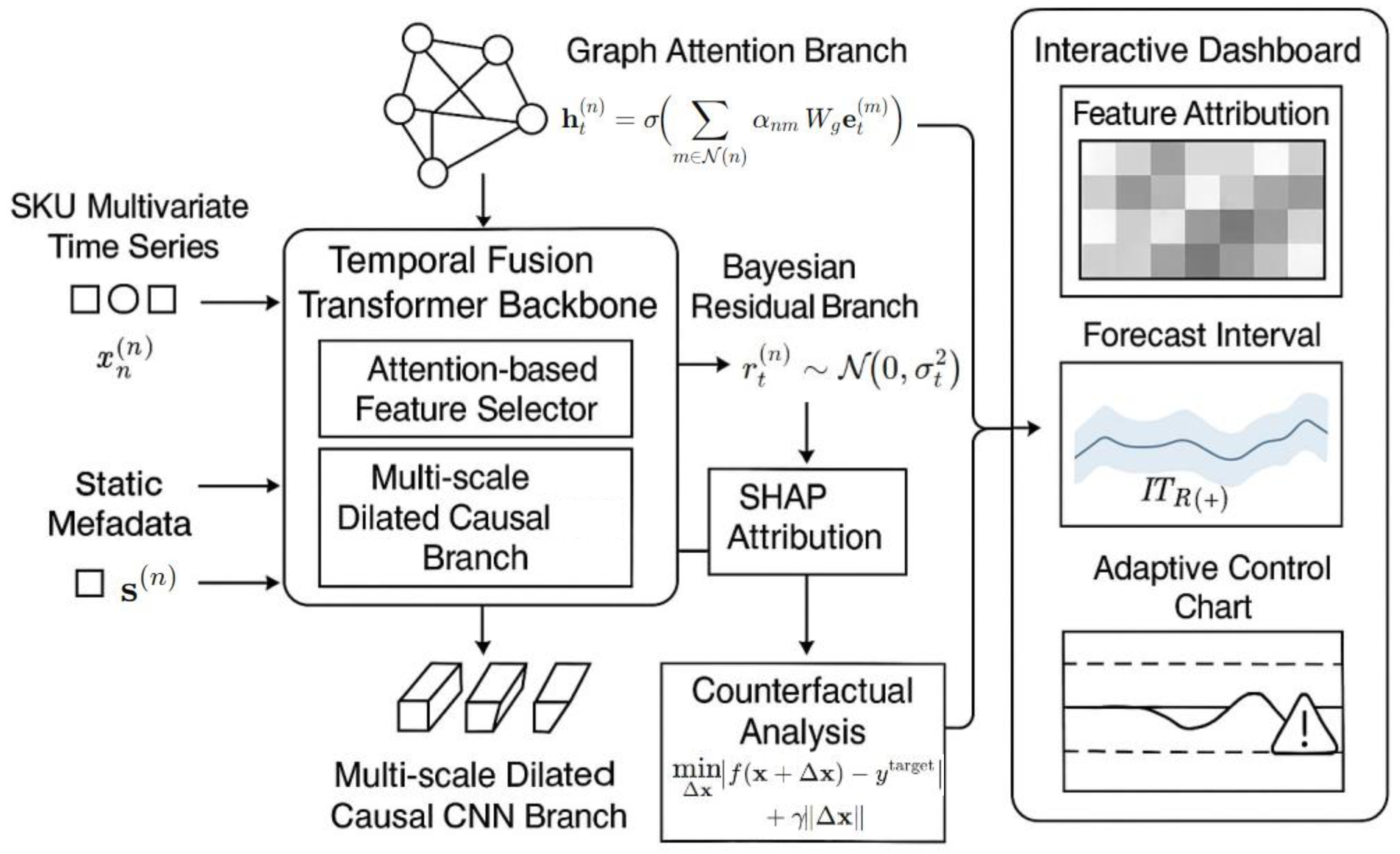
Figure 2.
Hourly Add-to-Cart vs Transaction Trend.
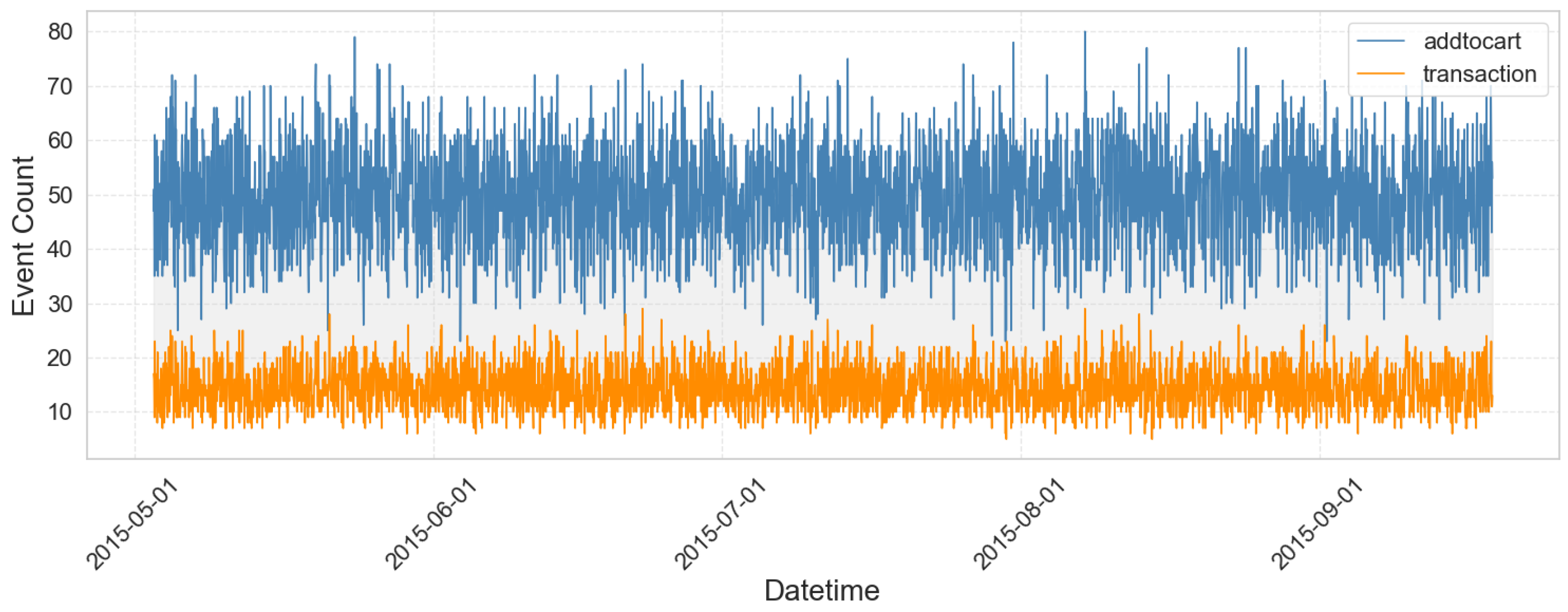
Figure 3.
Feature Attribution Comparison Across Models.
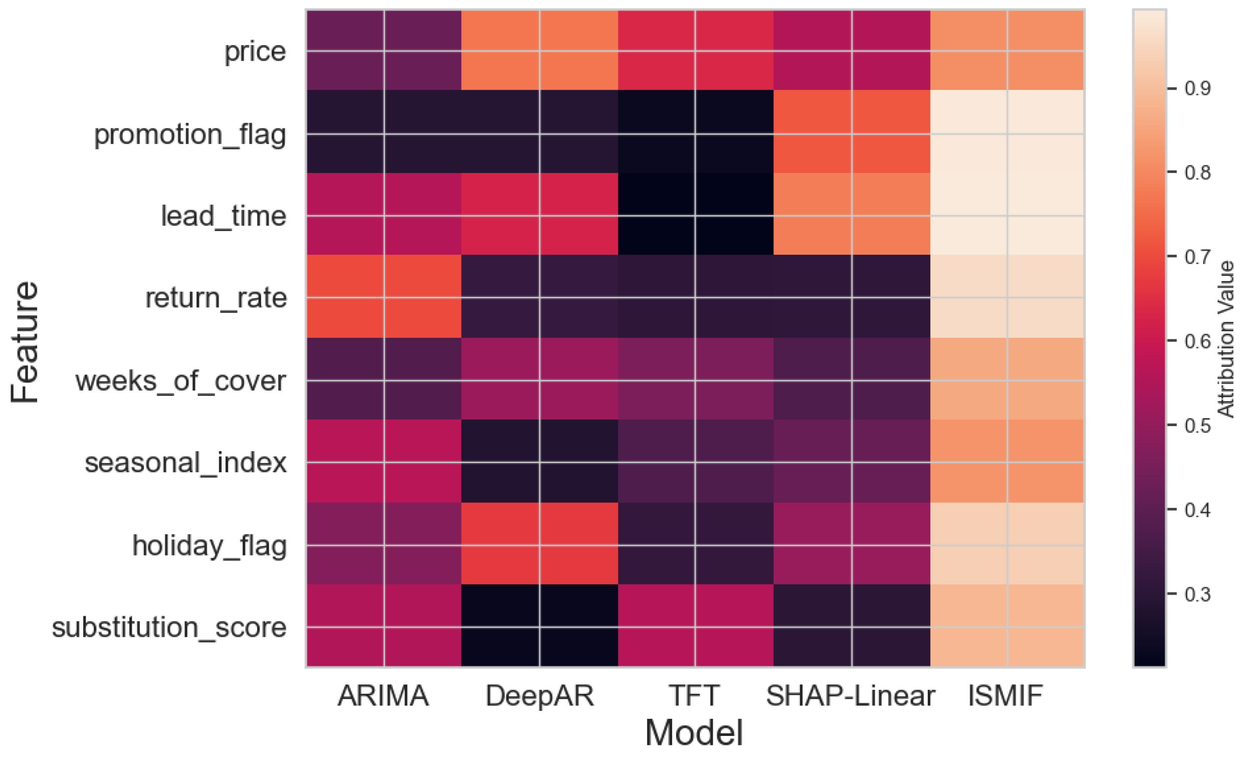
Figure 4.
Inventory Turnover Rate With Prediction Horizon.
Disclaimer/Publisher’s Note: The statements, opinions and data contained in all publications are solely those of the individual author(s) and contributor(s) and not of MDPI and/or the editor(s). MDPI and/or the editor(s) disclaim responsibility for any injury to people or property resulting from any ideas, methods, instructions or products referred to in the content. |
© 2025 by the authors. Licensee MDPI, Basel, Switzerland. This article is an open access article distributed under the terms and conditions of the Creative Commons Attribution (CC BY) license (http://creativecommons.org/licenses/by/4.0/).
Copyright: This open access article is published under a Creative Commons CC BY 4.0 license, which permit the free download, distribution, and reuse, provided that the author and preprint are cited in any reuse.


