Cryptocurrencies and Dependence: A Nonparametric View

1. Introduction

Cryptocurrencies have attracted a lot of attention since Bitcoin came into operation back in 2009, especially when investment banks endorsed it and the first futures and options started trading on the Chicago Mercantile Exchange (CME). Many researchers have focused on the modeling side of cryptocurrencies as an economic product or financial asset, while others have tried to quantify the relation between stocks and cryptocurrencies using different econometric tools.

On the theoretical side, Schilling and Uhlig (2019) discuss monetary policy in an economy with the dollar and Bitcoin as competing currencies and derive a pricing equation for the latter, showing that it is a martingale. Other theoretical models have been developed to explain the price dynamics of cryptocurrencies, as in Sockin and Xiong (2023), most taking into account network effects that drive risk and returns, such as Liu and Tsyvinski (2020), as well as common risk factors such as Liu et al. (2022).

On the econometric modeling side, cryptocurrencies have been investigated in their ability to work, in addition to common stocks (or other assets like gold and dollars), as mediating portfolio risk, that is, for diversification purposes. Different econometric tools have been employed; the asymmetric GARCH model of Dyhrberg (2016) showed that Bitcoin’s volatility behaves similarly to gold and dollar in having similar hedging capabilities and reacting symmetrically to good and bad news in an exponential GARCH model. Overall, Dyhrberg concludes that Bitcoin can be used as a tool for risk-averse investors in anticipation of bad news. Bouri et al.(2018), using a smooth transition VAR GARCH-in-mean model, showed that Bitcoin returns behave similarly to commodities and in addition, using different market volatility regimes, spillover effects add to Bitcoin’s volatility. Mariana et al.(2021), using daily data for Bitcoin, Ethereum, $S\&P500$ and gold spot prices during the COVID19 pandemic period (July 1, 2019, until April 6, 2020) and employing the Dynamic Conditional Correlation GARCH (1,1) model of Engle (2002), show that Ethereum is a better safe-haven asset than Bitcoin especially during short extreme stock market downturns, but it exhibits higher return volatility than Bitcoin. Both cryptocurrency returns however, display significantly higher volatility than gold and $S\&P500$. Recently, Li and Miu (2023) proposed a regime-switching approach where volatility and correlation parameters are jointly estimated and the volatility regime, the segmentation (high versus low), is endogenously determined by the market return data. Using their sophisticated approach, they conclude that although correlations are weak (even negative) most of the time, they switch to being significantly positive in the high volatility market regime, therefore cryptocurrencies can not be a safe haven for stock investors, having no risk-mitigation role during market downturns when investors need it the most.

Moving to studies on the statistical properties of cryptocurrencies such as dependence, Chaim and Laurini (2019), using three years of daily prices of nine cryptocurrencies from 2015 to 2018, employ a multivariate stochastic volatility model with jumps to capture the volatility dynamics proving the existence of two high volatility periods in 2017 and early 2018 with many outliers and high kurtosis coefficients. We note that they are using Pearson’s correlation coefficient as a dependence measure. Naeem et al.(2020), using a copula-GARCH model with the Gumbel, Clayton and SJC copulas, investigated the return-volume relation between three cryptocurrencies (Bitcoin, Ethereum and Litecoin) and showed asymmetric tail dependencies. Ahn (2022), similarly uncovered asymmetric tail dependence patterns using three cryptocurrencies (Bitcoin, Ethereum and BNB) and the $S\&P500$ with the help of exceedance conditional correlations measures, while Yen et al.(2023) investigated the effect of an economic policy uncertainty measure on the dependency between Bitcoin and 19 other cryptocurrencies. They constructed a Bitcoin index based on the strength of Pearson’s correlation and an average of the remaining 19 other cryptocurrencies, showing that an increase in global economic policy uncertainty strengthens the dependency effect of other cryptocurrencies on Bitcoin.

In this article, we focus on the tail dependence properties of cryptocurrency returns, by estimating non parametrically copula densities between pairs of cryptocurrencies. We complement this literature in using nonparametric estimators of copula density functions to visualize tail dependence patterns among the 10 most traded cryptocurrencies as in February 2025, taken from the website $https://coinmarketcap.com/$. We avoid using parametric copula functions as in Naeem et. al.(2020), worrying of possible misspecification problems, by choosing from a large collection of nonparametric copula kernel density estimator methodologies such as the beta kernels approach of Chen (1999), the transformation method of Geenens (2014), Charpentier et al.(2014) and Wen and Wu (2020), as well as the more recent one of orthogonal polynomials in Bakam and Pommeret(2023). Such methods have the advantage that the tail dependence between cryptocurrencies’ returns can be plotted, making the existence of possible asymmetric dependencies easy to visualize. All methodologies employed in this paper, are explained in some detail in order to help practitioners familiarize themselves with the latest in this interesting statistical literature and pick the method that suit their own need. The advantage of our approach over existing studies, is in the flexibility in that there is no need to select and fit some specific copula function as in Naeem et al.(2020) and fitting, is not as complicated and time consuming like the stochastic volatility model of Chaim and Laurini (2019). In addition, we are analyzing 10 cryptocurrencies and not as few as they did. We are also providing more robust measures of dependence, “model-free” as in Ahn (2022), in quantifying correlations between cryptocurrencies’ returns, contrary to Chaim and Laurini (2019) and Yen et al.(2023), that used Pearson’s correlation coefficient that can only capture linear dependencies. In our data analysis, using more sophisticated dependent measures that can capture non-linear dependencies (nonparametric in nature) such as Spearman’s, Kendall’s and the correlation coefficient of Bergsma and Dassios (2014) and Chatterjee (2021), we show that Pearson’s correlation coefficient can give misleading results both in terms of magnitude and direction of correlations. All correlation coefficients are carefully reviewed and explained.

2. Copula Density Estimation

2.1. Copula Functions

The modeling of the joint co-variation between random variables has been a hot research topic in recent years, especially in finance. In particular, classic dependence statistics such as correlation and covariance, suffer from serious shortcomings; see Embrechts et al. (2001). For example, Pearson’s correlation coefficient only measures linear relationship between random variables X and Y, while if the relationship is not linear then the result is inaccurate. In addition, the correlation is meaningless when it comes to categorical data. It would be nice to have some dependence modeling approach not sensitive to the assumption of joint normality (not supported by many data sets) and not conflating both marginal and joint distributions but providing a clean and independent separation between them. This is indeed achieved by the use of copula functions.

For simplicity, consider two random variables X and Y with distribution functions $F_X\left(x\right)=\mathbb{P}(X\le x)$ and $G_Y\left(y\right)=\mathbb{P}(Y\le y)$. To each pair of real numbers $(x,y)$ we can associate three numbers: $F_X\left(x\right)$, $G_Y\left(y\right)$ and $H(x,y)$. Each of these numbers lies in the interval $[0,1]$ and each pair $(x,y)$ leads to the point $(F_X\left(x\right),G_Y\left(y\right))$ in the unit square $[0,1]\times [0,1]$ due to the Integral Transformation Theorem. In its turn, this ordered pair corresponds to a number $C(x,y)$ in $[0,1]$. This correspondence between ordered pairs $(F_X\left(x\right),G_Y\left(y\right))$ and $C(x,y)$ is a function, called the Copula function. We now give a formal definition of a copula function.

Definition 1.

A function $C:{[0,1]}^d\to [0,1]$ is called a d-dimensional copula if there exists a random vector $(U_1,\dots ,U_d)$ with $U_j\sim U[0,1]$ for $j=1,\dots ,d$, such that

$$\mathbb{P}(U_1\le u_1,\dots ,U_d\le u_d)=C(u_1,\dots ,u_d).$$

Therefore the copula function $C(u_1,\dots ,u_d)$ is the cumulative distribution function of the realization $(u_1,\dots ,u_d)$ of the random vector $(U_1,\dots ,U_d)$. The usefulness of copula functions is due to Sklar’s Theorem that allows a multivariate distribution function to be split into its margins and a copula.

Theorem 1.

For F a continuous d-dimensional distribution function with margins $F_1,\dots ,F_d$, there exists a unique d-dimensional copula function C such that for all $(x_1,\dots ,x_d)\in {\mathbb{R}}^d$, we have

$$F(x_1,\dots ,x_d)=C\left(F_1\left(x_1\right),\dots ,F_d\left(x_d\right)\right).$$

Conversely, if C is a d-dimensional copula function and $F_1,\dots ,F_d$ are univariate distribution functions, then $F(x_1,\dots ,x_d)$ is a d-dimensional distribution function.

Although copula functions enjoy many properties, we state here the ones relevant to us.

• (P.1) The copula C is non-decreasing in each argument.;
• (P.2) The copula C is uniformly continuous in its domain;
• (P.3) All partial derivatives of the copula C exist
• (P.4) Invariance: If f and g are strictly increasing almost surely on the range of random variables X and Y respectively, then $C_{f\left(X\right),g\left(Y\right)}=C_{XY}$, that is, the copula function $C_{XY}$ is invariant under strictly increasing transformations of X and Y;
• (P.5) The copula C density exists everywhere in ${[0,1]}^2$ and is non-negative.

(P.1) is a property of a distribution function, (P.2) is useful in proving some theoretical properties of copulas, (P.3) allows us to define conditional distribution functions, like $\mathbb{P}(X\le x|Y\le y)=\partial C(u,v)/\partial v$, where $v=G\left(y\right)$ with G the marginal distribution function of Y. (P.4) is very useful because we can transform the cryptocurrency prices to returns using the log transformation without affecting the copula; the invariance property yields $C_{XY}=C_{log\left(X\right)log\left(Y\right)}$. (P.5) assures us on the existence of a copula density function. For further properties of copula functions, proofs, and more mathematical details, see Nelsen (1999), Trivedi and Zimmer (2005), McNeil, Frey and Embrechts (2005), Joe (2015) and Hofert et al. (2018), among others.

Some benefits of the copula approach in modeling dependencies between random variables are the following:

• (a) Any joint distribution can be “glued together” by two marginals and a copula;
• (b) The copula function is unique assuming continuous marginal distributions;
• (c) The joint dependence can be fully characterized by the copula function separately from the marginals;
• (d) The visualization of (especially) bivariate relations via the copula approach can offer precious insights concerning their dependence structure;
• (e) Robust measures of dependence like the Spearman’s rho coefficient and the Kendall’s tau coefficient that are not measuring only linear dependence, can be easily calculated via the copula function.

2.2. Kernel Copula Density Estimation

Using Sklar’s Theorem, we can construct copula functions simply by inverting the functional relation given by the theorem. Then, we get

$$C(u_1,\dots ,u_d)=F(F_1^{-1}\left(u_1\right),\dots ,F_d^{-1}\left(u_d\right)).$$

From the above, we can obtain the density of the Copula function. For simplicity, consider the bivariate case and note that we have,

$$C(\underset{u_1}{\underbrace{F_1\left(x_1\right)}},\underset{u_2}{\underbrace{F_2\left(x_2\right)}})=F(x_1,x_2)=F\left(\right(F_1^{-1}\left(u_1\right),\left(F_2^{-1}\left(u_2\right)\right),$$

Using the chain-rule, we get

$${\displaystyle \frac{\partial C(u_1,u_2)}{\partial u_1}}={\displaystyle \frac{\partial F(x_1,x_2)}{\partial x_1}}{\displaystyle \frac{\partial u_1}{\partial x_1}}={\displaystyle \frac{f(x_1,x_2)}{f_1\left(x_1\right)}}={\displaystyle \frac{f(F_1^{-1}\left(u_1\right),F_2^{-1}\left(u_2\right))}{f_1\left(F_1^{-1}\left(u_1\right)\right)}}.$$

Similarly, we have ${\displaystyle \frac{\partial C(u_1,u_2)}{\partial u_2}}={\displaystyle \frac{f(F_1^{-1}\left(u_1\right),F_2^{-1}\left(u_2\right))}{f_2\left(F_2^{-1}\left(u_2\right)\right)}}$, and putting these calculations together gives the density of a bivariate copula function,

$$c(u_1,u_2)={\displaystyle \frac{f(F_1^{-1}\left(u_1\right),F_2^{-1}\left(u_2\right))}{f_1\left(F_1^{-1}\left(u_1\right)\right)·f_2\left(F_2^{-1}\left(u_2\right)\right)}}.$$

Generalizing, we get the d-dimensional copula density function,

$$c(u_1,\dots ,u_d)={\displaystyle \frac{f(F_1^{-1}\left(u_1\right),\dots ,F_d^{-1}\left(u_d\right))}{{\prod }_{j=1}^d{f}_i\left(F_j^{-1}\left(u_j\right)\right)}}.$$

To estimate the above, consider again the density of the bivariate copula function $c(u,v)={\displaystyle \frac{{\partial }^{2}C}{\partial u\partial v}}(u,v)$ for $u,v\in [0,1]$ where $C(u,v)$ is the copula function itself. Assuming we have i.i.d. copies of ${\{U_i,V_i\}}_{i=1}^n$ from the copula C, we want to estimate the density c. We will review past and more recent methodologies such as the naive estimator of kernel density-type, the mirror-reflection estimator of Gijbels and Mielniczuk (1990), beta kernels estimator of Chen (1999), the Bernstein polynomials copula of Sancetta and Satchell (2004), transformation-type estimators, Loader (1996), Hjort and Jones (1996), Fermanian and Scaillet (2007), Geenens (2014), Charpentier et al. (2014) and Wen and Wu (2020) and the orthogonal projections estimator of Bakam and Pommeret (2023). Of course, this does not exhaust the literature as there are other estimators we do not discuss here.1

Starting with a kernel density-type copula estimator, for a sample $\{(U_i=F_X\left(X_i\right),V_i=F_Y\left(Y_i\right)),i=1,\dots ,n\}$, we have

$${\widehat{c}}^{*}(u,v)={\displaystyle \frac{1}{{n\left|\mathbf{N}\right|}^{1/2}}}\sum _{i=1}^n\mathbf{K}\left({\mathbf{H}}_{UV}^{-1/2}\left(\begin{array}{c}u-U_i\\ v-V_i\end{array}\right)\right),$$

where $\mathbf{K}:{\mathbb{R}}^2\to \mathbb{R}$ is a bivariate kernel function and ${\mathbf{H}}_{UV}$ a symmetric and positive definite bandwidth matrix. The problem with this estimator is that it is heavily affected by values at the border and at the corners of the $(u,v)$-values. In particular, it can be shown that on the corner values,2 we have

$$\mathbb{E}\left({\widehat{c}}^{*}(u,v)\right)={\displaystyle \frac{1}{4}}c(u,v)+\mathrm{O}\left(h\right),$$

while on the border values,3

$$\mathbb{E}\left({\widehat{c}}^{*}(u,v)\right)={\displaystyle \frac{1}{2}}c(u,v)+\mathrm{O}\left(h\right).$$

For a point close to the boundary of the unit square, the naive kernel estimator will put a significant amount of probability mass outside the unit square, hence ${\widehat{c}}_n$ cannot be a density function since it cannot integrate to 1 over ${[0,1]}^2$. So, to make ${\widehat{c}}_n$ be a density, we need to gather all the probability mass from outside the unit square and redistribute it back to ${[0,1]}^2$. We can augment data as follows,

$${\{{\tilde{U}}_{ik},{\tilde{V}}_{ik}\}}_{k=1,\dots ,9}=\{(U_i,V_i),(-U_i,V_i),(U_i,-V_i),(-U_i,-V_i),$$

$$(U_i,2-V_i),(U_i,V_i),(2-U_i,V_i),(2-U_i,-V_i),(2-U_i,2-V_i)\}.$$

The Mirror-Reflection copula density estimator of Gijbels and Mielniczuk (1990) is given by

$${\widehat{c}}_n^{MR}(u,v)={\displaystyle \frac{1}{n}}\sum _{i=1}^N\sum _{k=1}^9{K}_{b_n}(u-{\tilde{U}}_{ik})K_{b_n}(v-{\tilde{V}}_{ik}).$$

This estimator is strongly consistent and asymptotically normal.

To deal with the boundary bias problem, Chen (1999) introduced the beta kernel estimator for a density function with known compact support [0,1]. This is given by

$${\widehat{f}}_h\left(x\right)={\displaystyle \frac{1}{n}}\sum _{i=1}^{n}K\left(X_i,\underset{\alpha }{\underbrace{{\displaystyle \frac{x}{h}}+1}},\underset{\beta }{\underbrace{{\displaystyle \frac{1-x}{h}}+1}}\right),$$

for bandwidth $h>0$, with $K(·,\alpha ,\beta )$ the density of the beta distribution with parameters $\alpha ,\beta$, given by

$$K(x,\alpha ,\beta )={\displaystyle \frac{x^{\alpha }{(1-x)}^{\beta }}{B(\alpha ,\beta )}},B(\alpha ,\beta )={\displaystyle \frac{\Gamma (\alpha +\beta )}{\Gamma \left(\alpha \right)\Gamma \left(\beta \right)}},$$

for the gamma function $\Gamma \left(x\right)={\int }_0^{\infty }{t}^{x-1}{e}^{-t}dt$. The advantages of this method are, (a) it can match the compact support of the object to be estimated and (b) it has a flexible form and changes the smoothness as we move away from the boundaries. The Beta-kernel estimator of the copula density, using product beta kernels is given by

$${\widehat{c}}_n^B={\displaystyle \frac{1}{n}}\sum _{i=1}^{n}K\left(U_i,{\displaystyle \frac{u}{b_n}}+1,{\displaystyle \frac{1-u}{b_n}}+1\right)K\left(V_i,{\displaystyle \frac{v}{b_n}}+1,{\displaystyle \frac{1-v}{b_n}}+1\right),$$

where $K(x,\alpha ,\beta )$ is the density of a $Beta(\alpha ,\beta )$-distributed random variable evaluated at x.

Another way to deal with the problems of the naive kernel approach, is the Transformation method. The idea is to transform the data first so that its distribution (which is bounded) is supported on the full ${\mathbb{R}}^2$, then apply to the transformed data standard kernel estimation methods and finally back-transform the estimate to its original support. In more detail, we start with $(U,V)=(F_X\left(x\right),F_Y\left(y\right))$ whose margins are Uniformly distributed and we construct new random variables $X^{\prime }={\Phi }^{-1}\left(U\right),Y^{\prime }={\Phi }^{-1}\left(V\right)$. By Sklar’s Theorem, the bivariate density of a random vector can be written as

$$f(x,y)=c(\Phi (x),\Phi (y\left)\right)\varphi \left(x\right)\varphi \left(y\right).$$

Using pseudo-observations ${\left\{(U_i^{\prime },V_i^{\prime })\right\}}_{i=1}^n$ for $(U,V)$ we set ${\Phi }^{-1}\left(U_i^{\prime }\right)=X_i^{\prime }$, ${\Phi }^{-1}\left(V_i^{\prime }\right)=Y_i^{\prime }$ and first estimate

$$\widehat{f}(x,y)={\displaystyle \frac{1}{n{b}_n^2}}\sum _{i=1}^{n}K\left({\displaystyle \frac{x-X_i^{\prime }}{b_n}},{\displaystyle \frac{y-Y_i^{\prime }}{b_n}}\right).$$

Finally, estimate the copula density by

$${\widehat{c}}^{Tr}(u,v)={\displaystyle \frac{{\sum }_{i=1}^{n}K\left(\frac{{\Phi }^{-1}\left(u\right)-{\Phi }^{-1}\left(U_i^{\prime }\right)}{b_n},\frac{{\Phi }^{-1}\left(v\right)-{\Phi }^{-1}\left(V_i^{\prime }\right)}{b_n}\right)}{n{b}_n^2\varphi \left({\Phi }^{-1}\left(u\right)\right)·\varphi \left({\Phi }^{-1}\left(v\right)\right)}}.$$

Staying with the transformation approach, suggested in Loader (1996), Hjort and Jones (1996) and more recently in Geenens (2014), was to combine local likelihood density estimation methods together with the probit transformation. Analytically, the probit transformation uses the Normal quantile function ${\Phi }^{-1}$ to create a normalized i.i.d. random sample of pseudo-observations ${\widehat{U}}_i={\Phi }^{-1}\left({\widehat{U}}_i\right)$ and ${\widehat{V}}_i={\Phi }^{-1}\left({\widehat{V}}_i\right)$ and use them to obtain

$${\widehat{c}}^{\left(\tau \right)}(u,v)={\displaystyle \frac{{\widehat{f}}_{ST}({\Phi }^{-1}\left(u\right),{\Phi }^{-1}\left(v\right))}{\varphi \left({\Phi }^{-1}\left(u\right)\right)\varphi \left({\Phi }^{-1}\left(v\right)\right)}},S={\Phi }^{-1}\left(U\right),T={\Phi }^{-1}\left(V\right).$$

Then, a kernel-type copula density estimator is employed given by

$${\widehat{c}}^{\left(\tau \right)}(u,v)={\displaystyle \frac{1}{n|{\mathbf{H}}_{ST}{|}^{1/2}\varphi \left({\Phi }^{-1}\left(u\right)\right)\varphi \left({\Phi }^{-1}\left(v\right)\right)}}\sum _{i=1}^n\mathbf{K}\left({\mathbf{H}}_{ST}^{-1/2}\left(\begin{array}{c}{\Phi }^{-1}\left(u\right)-{\Phi }^{-1}\left({\widehat{U}}_i\right)\\ {\Phi }^{-1}\left(v\right)-{\Phi }^{-1}\left({\widehat{V}}_i\right)\end{array}\right)\right),$$

see Fermanian and Scaillet (2007), among others.

Although natural, an application of this procedure does not perform very well and a new idea by Geenens (2014) and Charpentier et al.(2014) was to combine the above approach with local likelihood density estimation methods which yields good and easy to implement estimators, fixing boundary issues and also coping with unbounded copula densities. In particular a polynomial approximation of order p for $log{f}_{ST}$ is given around $(s,t)\in {\mathbb{R}}^2$, by

$$LocalLogLinear:log{f}_{ST}(\tilde{s},\tilde{t})\approx a_{1,0}(s,t)+a_{1,1}(s,t)(\tilde{s}-s)+a_{1,2}(s,t)(\tilde{t}-t)$$

$$\equiv P_{{\mathbf{a}}_1}(\tilde{s}-s),a_{1,1}(s,t)(\tilde{t}-t),$$

$$LocalLogQuadratic:log{f}_{ST}(\tilde{s},\tilde{t})\approx a_{2,0}(s,t)+a_{2,1}(s,t)(\tilde{s}-s)+a_{2,2}(s,t)(\tilde{t}-t)$$

$$+a_{2,3}(s,t){(\tilde{s}-s)}^2+a_{2,4}(s,t){(\tilde{t}-t)}^2+a_{2,5}(s,t)(\tilde{s}-s)(\tilde{t}-t)$$

$$\equiv P_{{\mathbf{a}}_2}(\tilde{s}-s),a_{1,1}(s,t)(\tilde{t}-t).$$

The unknown coefficients above (all the a`s) are estimated by solving a weighted maximum likelihood problem, therefore obtaining an estimate of $f_{ST}$ that is then substituted in the copula density estimator yielding,

$${\widehat{c}}^{(\tau ,p)}(u,v)={\displaystyle \frac{{\tilde{f}}_{ST}^{\left(p\right)}({\Phi }^{-1}\left(u\right),{\Phi }^{-1}\left(v\right))}{\underset{“multiplie{r}^{”}}{\underbrace{\varphi \left({\Phi }^{-1}\left(u\right)\right)\varphi \left({\Phi }^{-1}\left(v\right)\right)}}}},S={\Phi }^{-1}\left(U\right),T={\Phi }^{-1}\left(V\right),$$

where, if $p=1$, we get the local log-linear fit while when $p=2$, we get the local log-quadratic fit. The asymptotic properties of the above estimators are derived in Charpentier et al.(2014) and a practical way of selecting the bandwidth parameters is devised as well as simulation studies compare this estimator to other competitors.

Recently, Wen and Wu (2020) proposed an improved transformation-kernel estimator that employs a smooth tapering device to correct for the erratic boundary behavior caused by the data transformation step and studied its asymptotic properties. Motivated by the “multiplier” term in the formula above that can grow without bound as u or v go to zero or one leading the estimator to become erratic near the boundaries, they introduced a tapering device thereby reducing the multiplier’s value at the boundaries. In particular, their modified multiplier term becomes

$${\left[{\varphi }_{1+{\theta }_1}\left({\varphi }^{-1}\left(u\right)\right){\varphi }_{1+{\theta }_1}\left({\varphi }^{-1}\left(v\right)\right)\right]}^{-1}\sim {\displaystyle \frac{exp(-{\theta }_1[{\left\{{\Phi }^{-1}\left(u\right)\right\}}^2+{\left\{{\Phi }^{-1}\left(v\right)\right\}}^2])}{\varphi \left({\Phi }^{-1}\left(u\right)\right)\varphi \left({\Phi }^{-1}\left(v\right)\right)}},$$

where $1+{\theta }_1$ with ${\theta }_1>0$ is the standard deviation of a normal density function. In addition, they introduce an adapted4 tapering through an interaction term on the numerator controlled by some parameter ${\theta }_2$, such that the modified transformation estimator becomes

$${\widehat{c}}^{MT}(u,v)={\displaystyle \frac{exp(-{\theta }_1[{\left\{{\Phi }^{-1}\left(u\right)\right\}}^2+{\left\{{\Phi }^{-1}\left(v\right)\right\}}^2]-\stackrel{interactionterm}{\overbrace{{\theta }_2{\Phi }^{-1}\left(u\right){\Phi }^{-1}\left(v\right))}}}{n·\eta ·\varphi \left({\Phi }^{-1}\left(u\right)\right)\varphi \left({\Phi }^{-1}\left(v\right)\right)}}\times$$

$$\times \sum _{i=1}^n{K}_h({\Phi }^{-1}\left(u\right)-{\widehat{S}}_i)K_h({\Phi }^{-1}\left(v\right)-{\widehat{T}}_i),$$

where $\eta$ is a normalization factor for the above density to integrate to one. The authors provide simplified formulas for the Gaussian kernel as well as asymptotic properties of their estimator.

Sancetta and Satchell (2004), introduced the Bernstein copula using Bernstein polynomials that are closed under differentiation. In the bivariate case, for a constant $\alpha \left({\displaystyle \frac{k_1}{m_1}},{\displaystyle \frac{k_2}{m_2}}\right)$, $k\in \{1,2\}$ with $1\le k\le m_i$, $i=1,2$, the Bernstein polynomials are given by

$$B_{k_i,m_i}\left(u_i\right)=\left(\begin{array}{c}{m}_1\\ k_1\end{array}\right)u_{ii}^k{(1-u_i)}_i^k,if{C}_B:{[0,1]}^2\to [0,1],$$

where

$$C_B(u,v)=\sum _{k_1=1}^{m_1}\sum _{k_2=1}^{m_2}\alpha \left({\displaystyle \frac{k_1}{m_1}},{\displaystyle \frac{k_2}{m_2}}\right)B_{k_1,m_1}\left(u_1\right)B_{k_2,m_2}\left(u_2\right).$$

It turns out that the Bernstein copula $C_B(u,v)$, satisfies the properties of a copula function. For more properties and mathematical details, see their paper.

The last method is that of orthogonal projection by Bakam and Pommeret (2023). Their estimator is based on so called orthonormal shifted Legendre polynomials, for $m\in \mathbb{N}$, given by

$$Q_m\left(x\right)=\sqrt{2m+1}\times \underset{shiftedLegendre}{\underbrace{L_m(2x-1)}},{\int }_I{Q}_m\left(x\right)Q_k\left(x\right)d\mu \left(x\right)={\delta }_{k,m},\left(orthonormalitycondition\right)$$

for Legendre polynomials defined by $L_0=1$, $L_1\left(x\right)x=x$ and $(m+1)L_{m+1}\left(x\right)=(2m+1)x{L}_m\left(x\right)-m{L}_{m-1}\left(x\right)$, with ${\delta }_{k,m}=1$ when $k=m$ and 0 elsewhere. Their (multivariate) copula density estimator becomes

$$c(u_1,\dots ,u_d)=\sum _{\mathbf{m}\in {\mathbb{N}}^d}{\rho }_m·{\mathbf{Q}}_{\mathbf{m}}\left(\mathbf{u}\right),{\mathbf{Q}}_{\mathbf{m}}\left(\mathbf{u}\right)=\prod _{j=1}^d{Q}_{m_j}\left(u_j\right),$$

with $\mathbf{m}={(m_1,\dots ,m_d)}^T$ the polynomial order that can be different for each on the d-dimensional random variables $\mathbf{u}=(u_1,\dots ,u_d)$, each in the unit interval, while ${\rho }_m=\mathbb{E}\left({\prod }_{j=1}^d{Q}_{m_j}\left(F_j\left(u_j\right)\right)\right)$, is a measure of all polynomial correlations between the marginal uniform random variables and in the two dimensional case (d=2) it is just a correlation between the two uniform random variables after having applied the shifted Legendre polynomial transformation on them. The authors provide information on the estimation of the above quantities, relations on their correlation measure to Spearman’s $\rho$ measure, as well as asymptotic properties for their estimators.

In the next section we review different dependence measures and how they can be computed, before we move on to the actual results.

3. Dependence Measures

Generally speaking, there are three types of dependence: linear, monotone and general. The most frequently used measure is the Pearsons’s correlation coefficient that is calculated for two variables X and Y and a sample of size n, by the formula

$$r_{X,Y}={\displaystyle \frac{{\sum }_{i=1}^n(X_i-\overline{X})(Y_i-\overline{Y})}{\sqrt{{\sum }_{i=1}^n{X}_i^2-n\overline{X}}\sqrt{{\sum }_{i=1}^n{Y}_i^2-n\overline{Y}}}}.$$

This coefficient is easy to interpret, being between -1 (perfect negative dependence) and 1 (perfect positive dependence) with 0 for independence, but it suffers from not being able to detect non-linear dependencies while also being affected by outliers. More robust measures of dependence have been devised that are based on nonparametric measures such as ranks. One such measure is Spearman’s correlation coefficient defined by

$${\widehat{\rho }}_S={\displaystyle \frac{{\sum }_{i=1}^n(R_i^X-{\overline{R}}^X)(R_i^Y-{\overline{R}}^Y)}{\sqrt{{\left[{\sum }_{i=1}^n(R_i^X-{\overline{R}}^X)\right]}^2{\left[{\sum }_{i=1}^n(R_i^Y-{\overline{R}}^Y)\right]}^2}}},$$

where $R_i^X$ stands for the rank $R_i$ of random variable X among the dataset $X_{1:n}$ 5. Compared to the Pearson’s correlation coefficient, it replaces the values of the data its ranks so is more robust. The formula for Spearman’s correlation coefficient can be simplified if we use the concept of relative ranks. The relative rank of $X_{1:n}$ with respect to $Y_{1:n}$ is given by $R_i^{X|Y}=rank\left(X_{O_i^Y}\right)$, where $O_{1:n}^Y$ denotes the orders of $Y_{1:n}$ 6 .

After some algebra, the formula becomes,

$${\widehat{\rho }}_S=\left(-{\displaystyle \frac{3(n+1)}{n-1}}\right)+\left({\displaystyle \frac{12}{n(n-1)}}\right)\left(\sum _{i=1}^n{\displaystyle \frac{i}{n+1}}{R}_i^{X|Y}\right).$$

Our next dependence measure is using the concept of signs. It is the Kendall’s correlation coefficient and is given by

$${\widehat{\rho }}_K={\displaystyle \frac{{\sum }_{i\ne j}({\psi }_{ij}^X-\overline{{\psi }^X})\left(({\psi }_{ij}^Y-\overline{{\psi }^Y})\right)}{\sqrt{{\sum }_{i\ne j}{({\psi }_{ij}^X-\overline{{\psi }^X})}^2{\sum }_{i\ne j}{({\psi }_{ij}^Y-\overline{{\psi }^Y})}^2}}},$$

where ${\psi }_{ij}^X=\mathit{sign}(X_i-X_j)$ for each $i,j$. A simplified formula is the following,

$${\widehat{\rho }}_K={\displaystyle \frac{1}{resizeboxwidth17.07713pt\left(\begin{array}{c}n\\ 2\end{array}\right)}}\underset{1\le i<j\le n}{\sum \sum }\mathit{sign}\left((X_i-X_j)(Y_i-Y_j)\right).$$

A more recent measure of correlation based on ranks is the Chatterjee’s correlation; Chatterjee (2021). To state its formula, we need first to arrange our bivariate sample

$$(X_{\left[1\right]},Y_{\left[1\right]}),(X_{\left[2\right]},Y_{\left[2\right]}),\dots ,(X_{\left[n\right]},Y_{\left[n\right]}),$$

such that $X_{\left[1\right]}<X_{\left[2\right]}<\dots <X_{\left[n\right]}$ and denote,

$$r_i=\sum _{j=1}^{n}1\{Y_{\left[j\right]}\le Y_{\left[i\right]}\}\mathrm{and}{l}_i=\sum _{j=1}^{n}1\{Y_{\left[j\right]}\ge Y_{\left[i\right]}\},$$

where $r_i$ is the rank of $Y_{\left[i\right]}$ and $l_i$, $i=1,\dots ,n$ are permutations of $1,\dots ,n$. We now give the sample Chatterjee’s correlation coefficient by

$${\widehat{\rho }}_{CJ}=1-{\displaystyle \frac{n}{2}}{\displaystyle \frac{{\sum }_{i=2}^n|r_i-r_{i-1}|}{{\sum }_{i=1}^n{l}_i(n-l_i)}}\stackrel{noties}{=}1-3{\displaystyle \frac{{\sum }_{i=2}^n|r_i-r_{i-1}|}{n^2-1}}.$$

Here, since this formula might be less familiar to the readers, we also state the population formula of Chatterjee’s correlation coefficient and give some intuitive explanation. We have,

$${\rho }_{CJ}={\displaystyle \frac{{\int }_{\mathbb{R}}Var\left\{\mathbb{E}\left(1\right\{Y\ge y\left\}\right|X)\right\}d{F}_Y\left(y\right)}{{\int }_{\mathbb{R}}Var\left\{1\{Y\ge y\}\right\}d{F}_Y\left(y\right)}},$$

and the intuition of the above formula is that now we are focusing on how much Y is a function of X which implies that (a) we are not interested in measuring a linear relation between our two variables and (b) it is not true that ${\rho }_{CJ}(X,Y={\rho }_{CJ}(Y,X)$ since we see in the formula that we have conditioned for the case of increasing values of X. Among other qualities of this new coefficient, are the following:

(1)

Under independence, we have $\sqrt{5n/2}·{\widehat{\rho }}_{CJ}\stackrel{D}{⟶}\mathcal{N}(0,1)$ (convergence in distribution);

(2)

${\rho }_{CJ}\in [0,1]$ and ${\rho }_{CJ}=0$ if and only if X and Y are independent, i.e. it is a strong correlation;

(3)

${\widehat{\rho }}_{CJ}\stackrel{\mathbb{P}}{⟶}{\rho }_{CJ}$ (convergence in probability).

Read their paper for more results.

The last measure of dependence is that of Bergsma and Dassios (2014), which is a strong correlation measure and modifies Kendall’s correlation. The sample Bergsma-Dassios covariance is given by the following V and U-statistics,

$${\widehat{\sigma }}_{BD}^V(X,Y)={\displaystyle \frac{1}{n^4}}\sum _{i_1,i_2,i_3,i_4=1}^n\alpha (X_{i_1},X_{i_2},X_{i_3},X_{i_4})·\alpha (Y_{i_1},Y_{i_2},Y_{i_3},Y_{i_4}),$$

$${\widehat{\sigma }}_{BD}^U(X,Y)={\displaystyle \frac{(n-4)!}{n!}}\sum _{1\le i_1,i_2,i_3,i_4\le n\&distinct}^n\alpha (X_{i_1},X_{i_2},X_{i_3},X_{i_4})·\alpha (Y_{i_1},Y_{i_2},Y_{i_3},Y_{i_4}),$$

respectively, where $\alpha (x,y,w,z)=sign\left(\right|x-y|+|w-z|-|x-w|-|y-z\left|\right)$. It turns out that the asymptotic distribution of the population Bergsma-Dassios covariance is given by

$$n·{\sigma }_{BD}^U(X,Y)\stackrel{D}{\to }{\displaystyle \frac{36}{{\pi }^4}}\sum _{i=1}^{\infty }\sum _{j=1}^{\infty }{\displaystyle \frac{1}{i^2{j}^2}}(W_{ij}-1),$$

where $W_{ij}$s are ${\chi }_1^2$-distributed random variables. Based on this result, we can test the null hypothesis that the correlation between X and Y is zero, that is $H_0:{\rho }_{BD}=0$ against $H_1:{\rho }_{BD}\ne 0$, where ${\rho }_{BD}(X,Y)={\sigma }_{BD}^U(X,Y)/\sqrt{{\sigma }_{BD}^U(X,X){\sigma }_{BD}^U(Y,Y)}$. Notice also that ${\rho }_{BD}(X,Y)$ is a strong correlation which means that ${\rho }_{BD}(X,Y)=0$ if and only if X and Y are independent. The only problem with this measure is that its calculation is computationally demanding.

4. Data Analysis

We are using daily data of the 10 most traded cryptocurrencies as in February 2025, taken from the website $https://coinmarketcap.com/$, converting the prices to returns by the log-transformation According to this website, the top 10 cryptocurrencies, in terms of market capitalization, were the following: Bitcoin (BTC), Etherium (ETH), Tether (USDT), XRP (XRP), Solana (SOL), BNB (BNB), USDC (USDC), Dogecoin (DOGE), Cardano (ADA) and Tron (TRX). We first display their historical prices from 1/1/2023 to 12/9/2024 as well as summary statistics.

We can see that most cryptocurrencies have rallied in 2024 with the exception of Tether and USDC, the last, displaying signs of stagnation except for a huge drop in price that occurred in the first quarter of 2023. We display summary statistics and dependence coefficients in the following tables.

Some comments on the above results are in order. Some currencies, like USDT and USDC have a limited band of price variations contrary to others like BTC and SOL for example. The correlation analysis, conducted pairwise, shows an interesting picture. The most popular crypto, Bitcoin, is highly positively correlated with ETC, SOL and TRX, while the negative correlation with USDT, although statistically significant using Pearson’s correlation coefficient, is negligible using the other correlation and dependence measures. In fact, during all correlation pairs, Pearson’s correlation often overstates the actual dependence as in the case of pairs BTC/BNB, XRP/BNB, XRP/ADA, BNB/USDC, BNB/TRX and ADA/TRX. For pair USDT/USDC, a negative Pearson correlation of -0.41 is actually slightly positive using Kendall’s and Spearman’s measures and near independent using Chatterjee’s measure, while the opposite holds for pairs BTC/USDC, XRP/USDC, SOL/USDC and USDC/DOGE. One therefore has to be very careful in using Pearson’s correlation coefficient as a measure of dependence.

Concerning the two most recent measures of dependence, Chatterjee and Bergsma-Dassios respectively, we can see that when their values are low, that is, close to zero, there is no dependence between cryptocurrency pairs even when the other three measures claim otherwise. This occurs with pairs BTC/USDC, ETC/USDC, USDT/ADA, XRP/DOGE, SOL/USDC, BNB/USDC and USDC/DOGE, so we still need to be cautious and subject our data to a battery of diverse tests in order to get a better picture on possible dependence patterns. We conclude by saying that since the Bergsma-Dassios measure requires $\mathrm{O}\left(n^4\right)$ operations, it is computationally demanding; however, recent research has improved that to $\mathrm{O}(n^2*log\left(n\right))$; see Weihs et al.(2016).

Figure 1. All cryptocurrency historical prices.

Figure 1. All cryptocurrency historical prices.

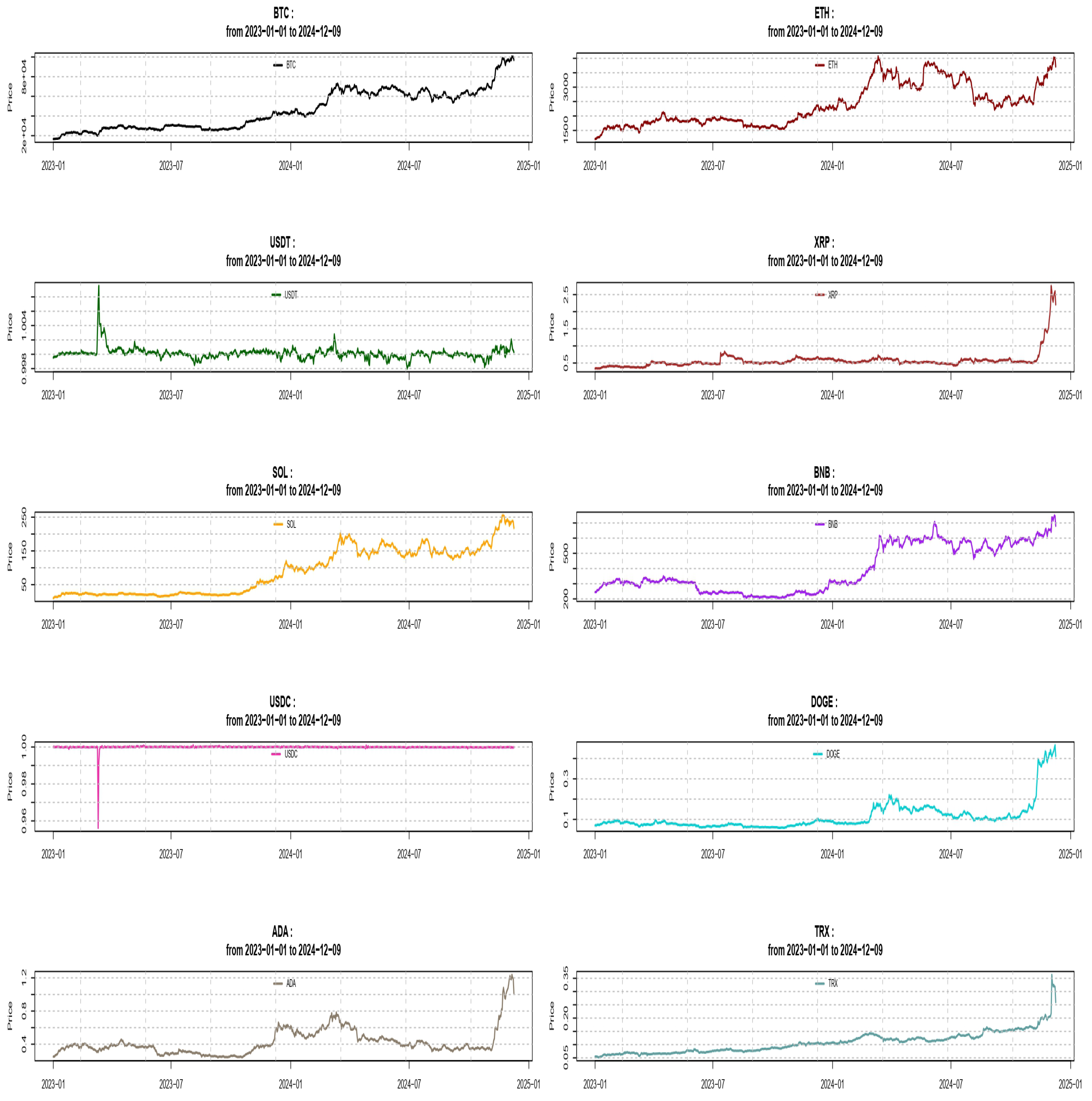
Table 1. Summary Statistics.

Summary Statistics
Coin	Minimum	1st Quarter	Median	Mean	3rd Quarter	Maximum
BTC	16595	27625	42155	45845	63420	100648
ETC	1200	1801	2239	2385	2999	4068
USDT	0.998	1.000	1.000	1.000	1.000	1.000
XRP	0.338	0.487	0.526	0.574	0.601	2.754
SOL	9.97	22.00	82.57	89.02	146.44	255.26
BNB	206	246	318	396	571	750
USDC	0.956	1.000	1.000	1.000	1.000	1.001
DOGE	0.0579	0.0734	0.0862	0.1116	0.1257	0.4656
ADA	0.240	0.329	0.379	0.421	0.464	1.238
TRX	0.0516	0.0763	0.1053	0.1080	0.1282	0.3631

Table 1. Summary Statistics.

Summary Statistics
Coin	Minimum	1st Quarter	Median	Mean	3rd Quarter	Maximum
BTC	16595	27625	42155	45845	63420	100648
ETC	1200	1801	2239	2385	2999	4068
USDT	0.998	1.000	1.000	1.000	1.000	1.000
XRP	0.338	0.487	0.526	0.574	0.601	2.754
SOL	9.97	22.00	82.57	89.02	146.44	255.26
BNB	206	246	318	396	571	750
USDC	0.956	1.000	1.000	1.000	1.000	1.001
DOGE	0.0579	0.0734	0.0862	0.1116	0.1257	0.4656
ADA	0.240	0.329	0.379	0.421	0.464	1.238
TRX	0.0516	0.0763	0.1053	0.1080	0.1282	0.3631

Table 2. Dependence Coefficients (i).

Dependence Coefficients
Pairs	Pearson	Kendall	Spearman	Chatterjee	Bergsma-Dassios
BTC/ETC	0.912***	0.803***	0.946***	0.760***	0.478***
BTC/USDT	-0.107***	-0.054**	-0.083**	0.230***	0.0101***
BTC/XRP	0.527***	0.408***	0.579***	0.503***	0.130***
BTC/SOL	0.982***	0.804***	0.937***	0.821***	0.497***
BTC/BNB	0.911***	0.617***	0.796***	0.691***	0.326***
BTC/USDC	0.021*	-0.241***	-0.354***	0.192***	0.056***
BTC/DOGE	0.810***	0.683***	0.846***	0.755***	0.382***
BTC/ADA	0.658***	0.437***	0.609***	0.539***	0.145***
BTC/TRX	0.890***	0.699***	0.886***	0.729***	0.385***
ETC/USDT	-0.120***	-0.049**	-0.080**	0.159***	0.0078***
ETC/XRP	0.393***	0.357***	0.515***	0.318***	0.105***
ETC/SOL	0.901***	0.696***	0.888***	0.653***	0.401***
ETC/BNB	0.855***	0.613***	0.814***	0.524***	0.296***
ETC/USDC	0.025	-0.217***	-0.324***	0.163***	0.045***
ETC/DOGE	0.678***	0.668***	0.852***	0.579***	0.351***
ETC/ADA	0.658***	0.526***	0.715***	0.452***	0.202***
ETC/TRX	0.710***	0.579***	0.808***	0.613***	0.319***
USDT/XRP	0.079**	0.048**	0.067*	0.059***	0.008***
USDT/SOL	-0.13***	-0.066***	-0.102***	0.0238	0.009***
USDT/BNB	-0.108***	-0.023**	-0.039**	0.0607***	0.011***
USDT/USDC	-0.411***	0.072***	0.097***	0.075***	0.0049***
USDT/DOGE	0.062*	-0.040*	-0.054*	0.031*	0.008***
USDT/ADA	0.142***	0.129***	0.189***	0.074***	0.0147***
USDT/TRX	-0.072*	-0.096***	-0.145***	0.088***	0.0127***
Statistical Significance: *10%, **5%, ***≤1%.

Table 2. Dependence Coefficients (i).

Dependence Coefficients
Pairs	Pearson	Kendall	Spearman	Chatterjee	Bergsma-Dassios
BTC/ETC	0.912***	0.803***	0.946***	0.760***	0.478***
BTC/USDT	-0.107***	-0.054**	-0.083**	0.230***	0.0101***
BTC/XRP	0.527***	0.408***	0.579***	0.503***	0.130***
BTC/SOL	0.982***	0.804***	0.937***	0.821***	0.497***
BTC/BNB	0.911***	0.617***	0.796***	0.691***	0.326***
BTC/USDC	0.021*	-0.241***	-0.354***	0.192***	0.056***
BTC/DOGE	0.810***	0.683***	0.846***	0.755***	0.382***
BTC/ADA	0.658***	0.437***	0.609***	0.539***	0.145***
BTC/TRX	0.890***	0.699***	0.886***	0.729***	0.385***
ETC/USDT	-0.120***	-0.049**	-0.080**	0.159***	0.0078***
ETC/XRP	0.393***	0.357***	0.515***	0.318***	0.105***
ETC/SOL	0.901***	0.696***	0.888***	0.653***	0.401***
ETC/BNB	0.855***	0.613***	0.814***	0.524***	0.296***
ETC/USDC	0.025	-0.217***	-0.324***	0.163***	0.045***
ETC/DOGE	0.678***	0.668***	0.852***	0.579***	0.351***
ETC/ADA	0.658***	0.526***	0.715***	0.452***	0.202***
ETC/TRX	0.710***	0.579***	0.808***	0.613***	0.319***
USDT/XRP	0.079**	0.048**	0.067*	0.059***	0.008***
USDT/SOL	-0.13***	-0.066***	-0.102***	0.0238	0.009***
USDT/BNB	-0.108***	-0.023**	-0.039**	0.0607***	0.011***
USDT/USDC	-0.411***	0.072***	0.097***	0.075***	0.0049***
USDT/DOGE	0.062*	-0.040*	-0.054*	0.031*	0.008***
USDT/ADA	0.142***	0.129***	0.189***	0.074***	0.0147***
USDT/TRX	-0.072*	-0.096***	-0.145***	0.088***	0.0127***
Statistical Significance: *10%, **5%, ***≤1%.

Table 3. Dependence Coefficients (ii).

Dependence Coefficients
Pairs	Pearson	Kendall	Spearman	Chatterjee	Bergsma-Dassios
XRP/SOL	0.457***	0.365***	0.556***	0.311**	0.113***
XRP/BNB	0.334***	0.146***	0.191***	0.186***	0.028***
XRP/USDC	0.024**	-0.069***	-0.103***	0.076***	0.005***
XRP/DOGE	0.763***	0.238***	0.362***	0.213***	0.049***
XRP/ADA	0.739***	0.285***	0.379***	0.261***	0.067***
XRP/TRX	0.701***	0.405***	0.5784***	0.373***	0.138***
SOL/BNB	0.915***	0.627***	0.818***	0.641***	0.325***
SOL/USDC	0.0105*	-0.282***	-0.416***	0.149***	0.065***
SOL/DOGE	0.766***	0.722***	0.896***	0.688***	0.393***
SOL/ADA	0.638***	0.463***	0.639***	0.497***	0.155***
SOL/TRX	0.861***	0.663***	0.865***	0.675***	0.379***
BNB/USDC	-0.006*	-0.301***	-0.447***	0.127***	0.076***
BNB/DOGE	0.705***	0.736***	0.904***	0.685***	0.391***
BNB/ADA	0.485***	0.473***	0.626****	0.441***	0.162***
BNB/TRX	0.751***	0.419***	0.659***	0.548***	0.205***
USDC/DOGE	0.0026*	-0.291***	-0.433***	0.118***	0.072***
USDC/ADA	0.0146*	-0.101***	-0.155***	0.043**	0.012***
USDC/TRX	0.020***	-0.261***	-0.371***	0.082***	0.0633***
DOGE/ADA	0.796***	0.574***	0.729***	0.574***	0.224***
DOGE/TRX	0.77***	0.456***	0.703***	0.527***	0.224***
ADA/TRX	0.653***	0.273***	0.433***	0.338***	0.086***
Statistical Significance: *10%, **5%, ***≤1%.

Table 3. Dependence Coefficients (ii).

Dependence Coefficients
Pairs	Pearson	Kendall	Spearman	Chatterjee	Bergsma-Dassios
XRP/SOL	0.457***	0.365***	0.556***	0.311**	0.113***
XRP/BNB	0.334***	0.146***	0.191***	0.186***	0.028***
XRP/USDC	0.024**	-0.069***	-0.103***	0.076***	0.005***
XRP/DOGE	0.763***	0.238***	0.362***	0.213***	0.049***
XRP/ADA	0.739***	0.285***	0.379***	0.261***	0.067***
XRP/TRX	0.701***	0.405***	0.5784***	0.373***	0.138***
SOL/BNB	0.915***	0.627***	0.818***	0.641***	0.325***
SOL/USDC	0.0105*	-0.282***	-0.416***	0.149***	0.065***
SOL/DOGE	0.766***	0.722***	0.896***	0.688***	0.393***
SOL/ADA	0.638***	0.463***	0.639***	0.497***	0.155***
SOL/TRX	0.861***	0.663***	0.865***	0.675***	0.379***
BNB/USDC	-0.006*	-0.301***	-0.447***	0.127***	0.076***
BNB/DOGE	0.705***	0.736***	0.904***	0.685***	0.391***
BNB/ADA	0.485***	0.473***	0.626****	0.441***	0.162***
BNB/TRX	0.751***	0.419***	0.659***	0.548***	0.205***
USDC/DOGE	0.0026*	-0.291***	-0.433***	0.118***	0.072***
USDC/ADA	0.0146*	-0.101***	-0.155***	0.043**	0.012***
USDC/TRX	0.020***	-0.261***	-0.371***	0.082***	0.0633***
DOGE/ADA	0.796***	0.574***	0.729***	0.574***	0.224***
DOGE/TRX	0.77***	0.456***	0.703***	0.527***	0.224***
ADA/TRX	0.653***	0.273***	0.433***	0.338***	0.086***
Statistical Significance: *10%, **5%, ***≤1%.

5. Copula Density Results

We apply all the methods mentioned in the theory section on different cryptocurrency return pairs and have plotted the specific method that shows the most clear and easy to interpret results on their tail dependence. Not all pairs are included in this section for economy of space. Note that on each plot, from Figure 2, Figure 3, Figure 4, Figure 5 and Figure 6, the header displays the crypto pair and the specific method applied that, in our opinion, gave the clearest results out of all methods tried.

We can see that BTC negative tail dependence is more pronounced when paired with ETC, XRP and SOL while positive tail dependence is stronger when paired with BNB, ADA and TRX. BTC tail dependence with USDT is more on the positive side while it is less conclusive when paired with USDC. Going to ETC, the second most popular cryptocurrency, negative tail dependence is dominant when paired with XRP, SOL, USDC and TRX while positive tail dependence is stronger when paired with BNB, DOGE and ADA. For other pairs included, it is interesting to notice the strong negative tail dependence between XRP and SOL, the strong positive tail dependence between pairs ADA-TRX and DOGE-SOL, the slightly positive dependence between USDC and DOGE and the tail symmetry displayed by the pair ADA and DOGE.

For the methods that seem to work better for our data, transformation-type methods are the best performers, estimated either with local linear or quadratic likelihood with different bandwidth selections, giving sharp tail plots. Older methods like the mirror-reflection and the use of beta kernels are not selected due to rough (more rounded) plots at the tails. Results using the Bernstein copula are displayed only for the pair DOGE-SOL where we can see the tail roughness in the plot. The orthogonal transformation with the use of shifted-Legendre polynomials, is displayed twice for pairs BTC-USDT and USDC-DOGE

Figure 2. Kernel Copula Densities: BTC vs USDT, XRP, SOL.

Figure 2. Kernel Copula Densities: BTC vs USDT, XRP, SOL.

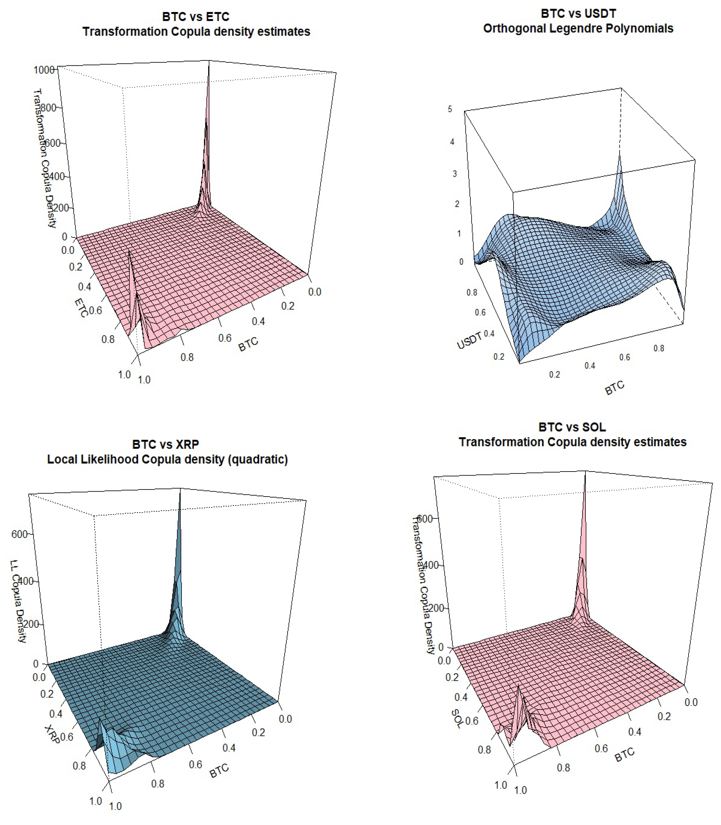
Figure 3. Kernel Copula Densities: BTC vs BNB, USDC, DOGE, ADA.

Figure 3. Kernel Copula Densities: BTC vs BNB, USDC, DOGE, ADA.

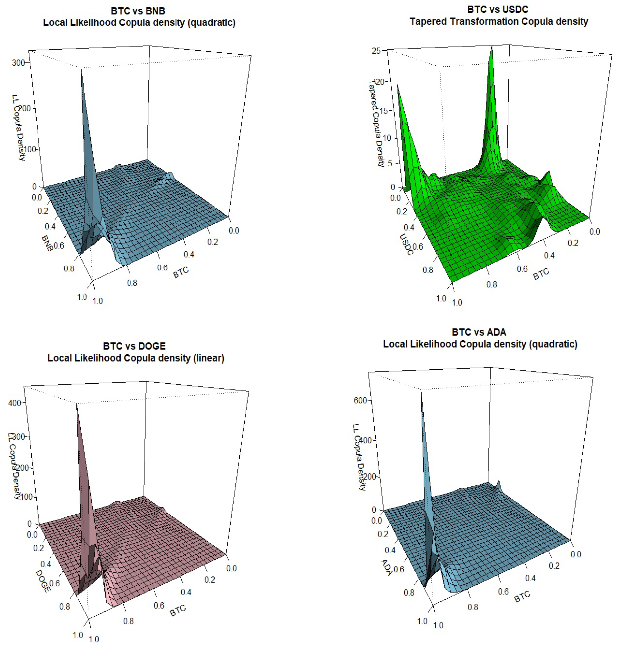
Figure 4. Kernel Copula Densities: ETH vs XRP, SOL, BNB.

Figure 4. Kernel Copula Densities: ETH vs XRP, SOL, BNB.

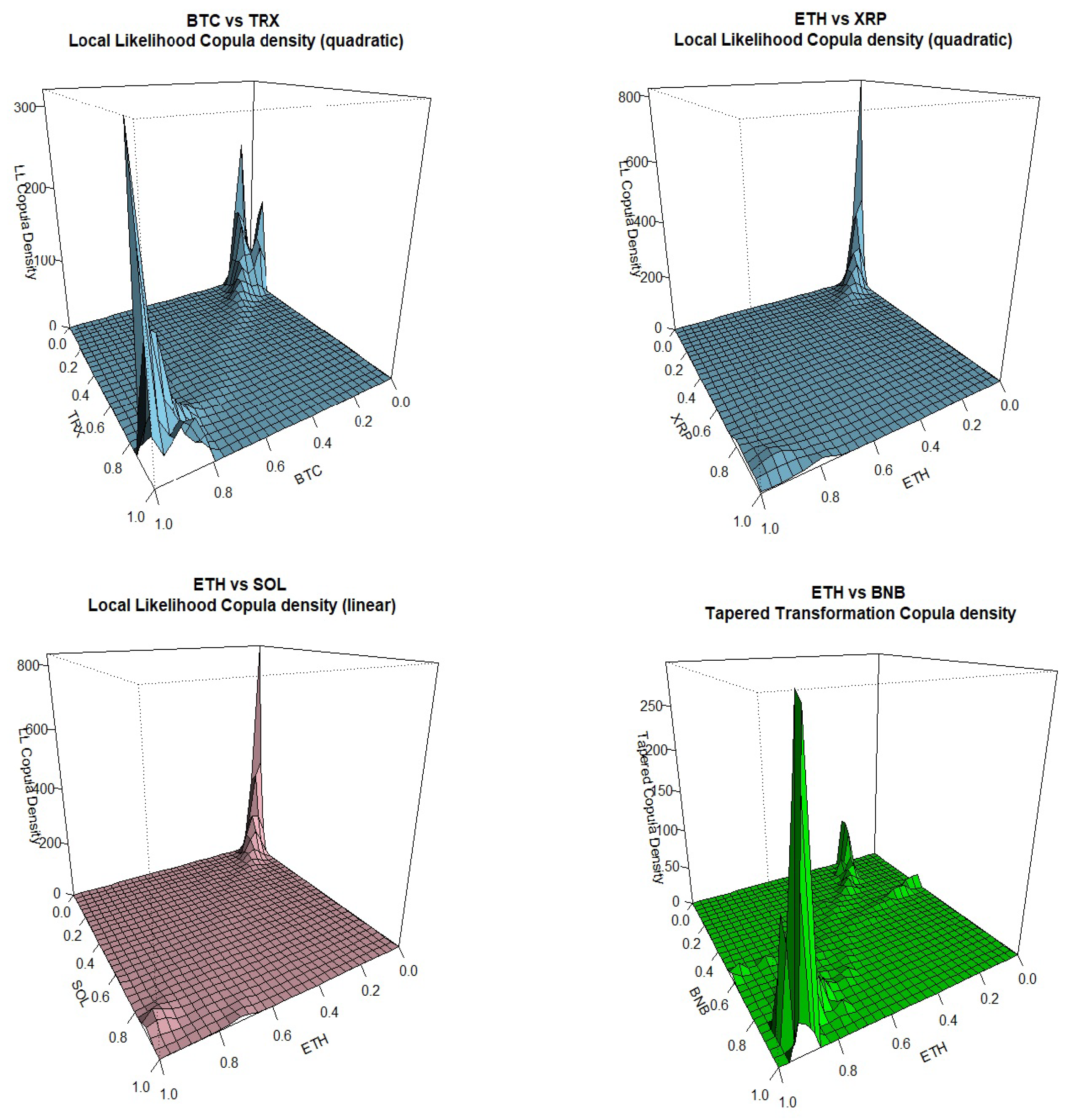
Figure 5. Kernel Copula Densities: ETH vs DOGE, ADA, TRX.

Figure 5. Kernel Copula Densities: ETH vs DOGE, ADA, TRX.

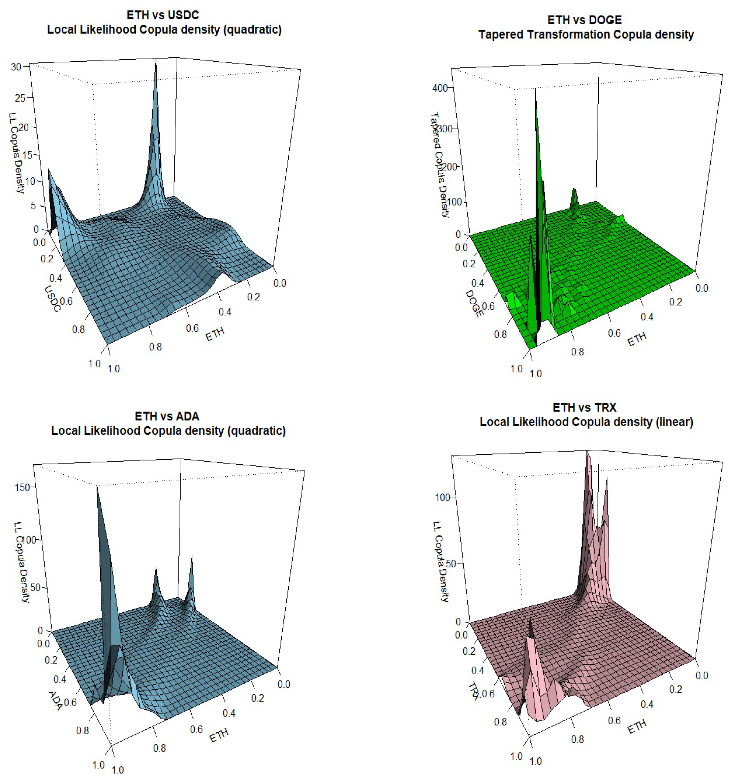
Figure 6. Kernel Copula Densities: Other pairs.

Figure 6. Kernel Copula Densities: Other pairs.

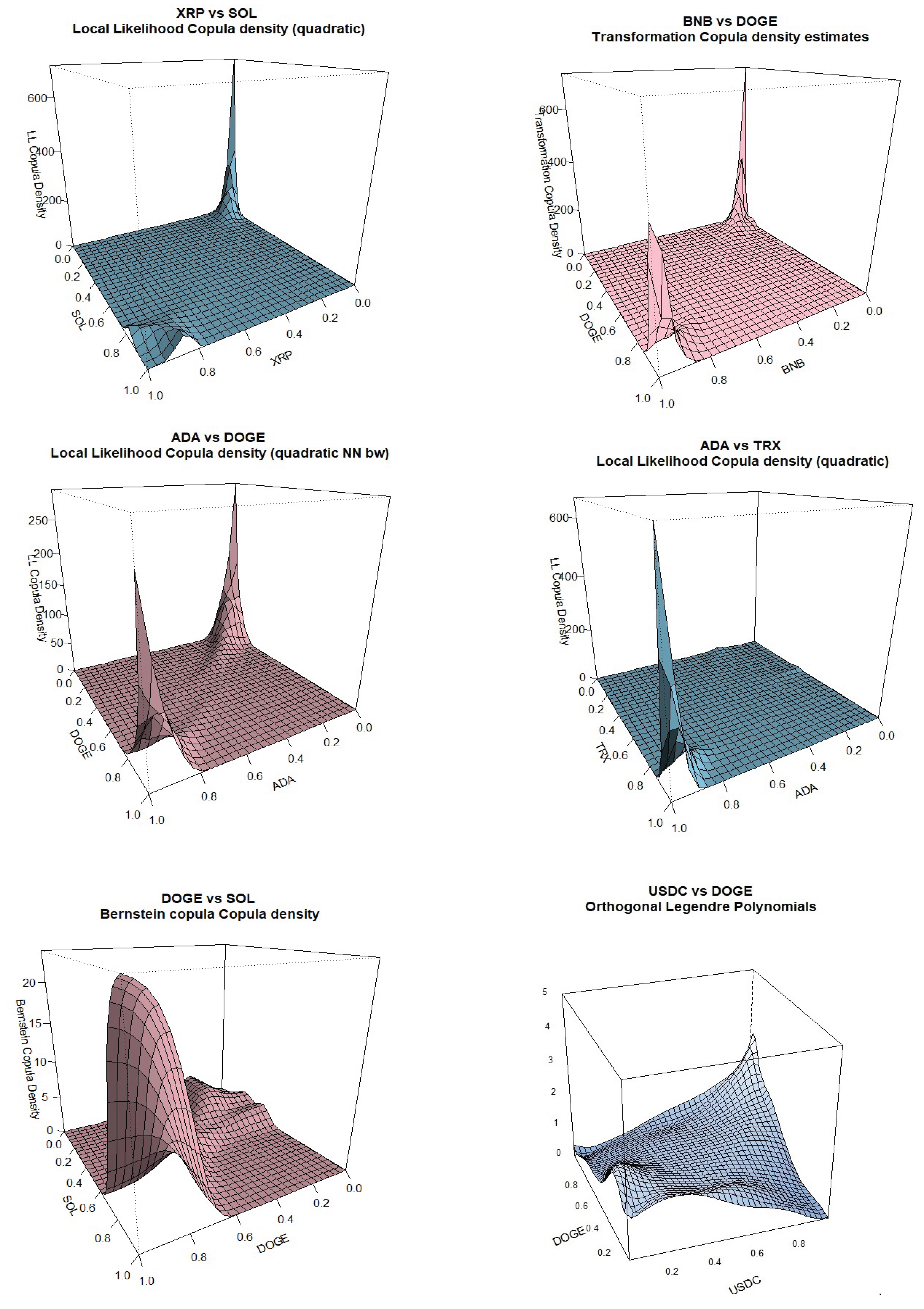
These results are interesting in that they can be used by investors that include cryptocurrencies in their portfolio for diversification purposes. One should avoid having positively dependent cryptocurrencies like BTC with BNB, ADA, DOGE and TRX, avoid ETH paired with BNB, DOGE and ADA and finally also avoid pairs like DOGE-SOL and USDC-DOGE. She better have in her portfolio cryptocurrency BTC together with ETC, XRP and SOL, or ETH together with XRP, SOL, USDC and TRX. For other pairs, XRP-SOL looks like a good idea.

Finally, the bivariate plots can point to the direction on which parametric copula model one can choose in estimating different tail dependence coefficients between cryptocurrency returns pairs, as in the textbook by Joe (2015). In this paper, we insist on using a nonparametric approach to describe tail dependence to avoid issues of misspecification and complicated tests for parametric copula model fit; see Hofert et al.(2018) for a textbook treatment.

6. Conclusion

In this paper, we have employed the latest research in the statistical estimation of nonparametric copula density function to uncover tail dependencies between pairs of cryptocurrency returns. First we have carefully reviewed some important methodologies in this active research area to make them better known to a wider audience in applied finance researchers and then we have used almost 2 years of daily data for the 10 most traded cryptocurrencies as in February 2025, and have plotted the copula densities for 20 pairs, showing asymmetric tail dependence patterns for most of them.

In addition, we have provided theory of different dependence, beyond the often used Pearson’s correlation coefficient which only captures linear dependence, and have shown that the last is inadequate in capturing data dependencies since it usually overestimates true data dependencies. Some of the dependent coefficients we examined, such as the Bergsma-Dassios’ covariance and Chatterjee’s correlation are the state of the art methodologies, robust for outliers, with good statistical properties and relatively easy to compute.

Although using nonparametric methods has the disadvantage of not being easy to interpret, on the other hand, it avoids misspecification problems when doing some parametric copula density estimation while it has the flexibility of applying many different methodologies and choosing the one that shows the most clear results. This approach can also be the first step, in that it can reveal the type of dependence patters between cryptocurrency returns, so that if one wants to further analyze the data by applying some more sophisticated model, can have an idea of the type of model to use. It would be of interest to split the data sample in different regimes based on the volatility or some other measure, like the occurrence of COVID19 event, and examine if the dependence pattern is different within each regime. We hope that by using this methodology, we have shed light to the issues of dependence between cryptocurrencies and other researchers can benefit from using such statistical methods.

References

- Ahn, Y., “Asymmetric tail dependence in cryptocurrency markets: A Model-free approach”, 2022, Finance Research Letters, Vo.47, 102746.
- Bakam, Yves I. Ngounou and D.Pommeret, “Nonparametric estimation of copulas and copula densities by orthogonal projections”, 2023, Econometrics and Statistics, Available online 29 April 2023.
- Bouri, E., M.Das, R.Gupta and R.Roubaud, “Spillovers between Bitcoin and other assets during bear and bull markets”, 2018, Applied Economics, Vol.50, pp.5935-5949.
- Chaim, P. and P.Laurini, “Nonlinear dependence in cryptocurrency markets”, 2019, North American Journal of Economics and Finance, Vol.48., pp.32-47.
- Charpentier, A., G. Geenens and D. Paindaveine, “Probit Transformation for Nonparametric Kernel Estimation of the Copula Density”, 2017, Bernoulli, Vol.23 (3), pp.1848-73.
- Chatterjee, S., “A New Coefficient of Correlation”, 2021, Journal of the American Statistical Association, Vol.116, No.536, pp.2009-22.
- Cherubini, U., E.Luciano and W.Vecchiato, “Copula Methods in Finance”, 2004, John Wiley and Sons.
- Dyhrberg, A.H., “Bitcoin, gold and the dollar - a GARCH volatility analysis”, 2016, Finance Research Letters, Vol.16, pp.85-92.
- Embrechts, P., A.J.McNeil, D.Straumann, “Correlation and Dependency in Risk Management: properties and pitfalls”, 2001, Department of Mathematics, ETHZ, Zurich, Working Paper.
- Engle, R., “Dynamic Conditional Correlation: A Simple Class of Multivariate Generalized Autoregressive Conditional Heteroskedasticity Models”, 2002, Journal of Business & Economic Statistics, Vol.20, No.3, pp.339-50.
- Fermanian, J-D. and O.Scaillet, “Nonparametric Estimation of Copulas for Time Series”, 2007, Journal of Risk, Vol.5, pp.25-54.
- Geenens, G., “Probit Transformation for Kernel Density Estimation on the Unit Interval ”, 2014, Journal of the American Statistical Association, Vol. 109, pp.346-358.
- Hofert, M., I.Kojadinovic, M.Machler and J.Yan, “Elements of Copula Modeling with R”, 2018, Springer.
- Hjort, N.L. and M.C.Jones, “Locally Parametric Nonparametric Density Estimation”, 1996, Annals of Statistics, Vol.24, pp.1619-1647.
- Joe, H., “Dependence Modeling with Copulas”, 2015, Chapman & Hall/CRC, Monographs on Statistics and Applied Probability.
- Li, L. and P.Miu, “Are cryptocurrencies a safe haven for stock investors? A regime-switching approach”, 2023, Journal of Empirical Finance, Vol.70, pp.367-385.
- Liu, Y. and A.Tsyvinski, “Risks and Returns of Cryptocurrency”, 2021, The Review of Financial Studies, Vol.34, pp.2689-2727.
- Liu, Y., A.Tsyvinski and X.Wu, “Common Risk Factors in Cryptocurrency”, 2022, The Journal of Finance, Vol.LXXVII, NO.2 pp.1133-1177.
- Loader, C.R., “Local Likelihood Density Estimation”, 1996, Annals of Statistics, Vol.24, pp.1602-1618.
- Mariana, C.D., I.A.Ekaputra and Z.A.Husodo, “Are Bitcoin and Ethereum safe-havens for stocks during the COVID-19 pandemic?”, 2021, Finance Research Letters, Vol.38, 101798.
- McNeil, A.J., R. Frey and P. Embrechts, “Quantitative Risk Management, concepts, techniques, tools”, 2005, Princeton Series in Finance.
- Myers, S., “Determinants of Corporate Borrowing”, 1977, Journal of Financial Economics, Vol.5, Issue 2, pp.147-175.
- Naeema, M., E.Bourib, G.Boakoc and D.Roubaudd, “Tail dependence in the return-volume of leading cryptocurrencies”, 2020, Finance Research Letters, Vol.36, 101326.
- Nagler, T., “kdecopula: An R Package for the Kernel Estimation of Bivariate Copula Densities”, 2018, Journal of Statistical Software Vol.84, 7, pp.1-22.
- Nelsen, R. B., “An Introduction to Copulas”, Lecture Notes in Statistics, 1999, Springer.
- Sancetta, A. and S.Satchell, “ The Bernstein copula and its applications to modeling and approximations of multivariate distributions”, 2004, Econometric Theory, Vol.20, 03, pp.535-62.
- Schilling, L. and H.Uhlig, “Some simple bitcoin economics”, 2019, Journal of Monetary Economics, Vol.106, pp.16-26.
- Sockin, M. and W.Xiong, “A Model of Cryptocurrencies”, 2023, Management Science, Vol.69, No.11, pp.6684-6707.
- Trivedi, P.K. and D.M.Zimmer, “Copula Modeling: An Introduction for Practitioners”, 2005, Foundations and Trends in Econometrics, Vol. 1, No 1, pp.1-111.
- Weihs, L., M.Drton and D.Leung, “Efficient Computation of the Bergsma-Dassios Sign Covariance”, 2016, Computational Statistics, Vol.31, Issue 1, pp.315-28.
- Wen, K. and X.Wu, “Transformation-Kernel Estimation of Copula Densities”, 2020, Journal of Business and Economic Statistics, Vol. 38,Issue 1, pp.148-164.
- Yen, K.-C., W.-Y.Nie, H.L..Chang and L.-H.Chang, “Cryptocurrency return dependency and economic policy uncertainty”, 2023, Finance Research Letters, Vol.56, 104182.