Submitted:
14 May 2025
Posted:
15 May 2025
You are already at the latest version
Abstract
This paper presents a comprehensive evaluation of the possible implementation of a CO2-enhanced oil recovery (CO2-EOR) strategy within a geologically heterogeneous reservoir, which was discovered in 1996 and initiated production in 2001. The field's geological framework comprises six distinct limestone layers, with data collection spanning seven drilled wells. The project reassesses the geological and simulation models of the field, implements a CO2-EOR screening process utilizing extensive methodologies, develops a detailed field-scale compositional reservoir flow model, and executes a history-matching exercise to refine the model based on actual production data. In addition, EOR development strategies, including waterflooding, continuous CO₂ injection, and water alternating gas (WAG) injection, are presented. In each scheme, multiple cases are run to determine the best operating conditions for field performance optimization. The reservoir simulation model was developed utilizing an integrated dataset comprising geophysical, geological, and engineering information, including three-dimensional surface seismic surveys, well log data, and fluid property analyses. A representative fluid sample extracted from the reservoir was subjected to detailed analysis and employed in the calibration of the equation of state to ensure accurate characterization of the reservoir fluids. The history-matched model was then used in the forecasting process under two main development scenarios, namely, the 3 injectors/3 producers’ custom pattern and the 12 injectors/6 producers’ five-spot inverted pattern. These were further categorized into three main divisions, including waterflooding, continuous CO₂ injection, and WAG. Based on the specific reservoir conditions, the operating parameters of the continuous CO₂ and WAG injections with 1:1 and 1:2 cycles were modified to achieve the highest oil recovery. Furthermore, the five-spot inverted infill drilling method produced more oil than the custom 3/3 method, and our economics show that the five-spot inverted infill drilling is more profitable but cost-intensive as compared to the custom method.
Keywords:
CO2-Enhance Oil Recovery
; Reservoir Simulation
; History Matching
; Water Alternating Gas (WAG)
; Infill Drilling
1. Introduction
As many mature oil fields face declining production and enter the tail-end phase after primary and secondary production, Enhanced Oil Recovery (EOR) methods, such as CO2 injection, have emerged as vital strategies to extract additional oil, extend field lifespans, and boost profitability [1,2]. Employing CO2 as a tertiary recovery method typically following water flooding has shown promising results globally, with potential incremental oil recoveries ranging from 7% to 15% of the original oil in place [2]. The geologically heterogeneous reservoir field suggests a similar recovery potential post-waterflood. Carbon dioxide Enhanced Oil Recovery (CO2-EOR) is a well-established technique that not only increases oil production but also contributes to environmental sustainability [1]. Interestingly, the majority of CO2 utilized in EOR processes is not merely circulated, it remains sequestered within the reservoirs, providing the dual benefit of enhancing oil recovery while mitigating the greenhouse gas emissions from fossil fuels. This aspect of CO2-EOR has gained relevance as concerns over atmospheric greenhouse gases primarily from anthropogenic sources have spurred the development of Carbon Capture Utilization and Sequestration (CCUS) technologies. For many years, waterflooding has been used as a simple and effective EOR technique. This technique involves the injection of water into the reservoir to displace oil toward production wells. As the injected water increases the reservoir pressure, it facilitates the movement of oil toward production wells. Moreover, waterflooding contributes to the maintenance of the reservoir pressure, a crucial factor for crude oil extraction [3]. Various factors, such as reservoir permeability, oil viscosity, and water quality, influence the effectiveness of waterflooding [4]. In reservoirs with low permeability or highly viscous oils, waterflooding may not always achieve optimal results [5]. Nonetheless, due to its simplicity and cost effectiveness, waterflooding remains the most widely employed EOR technique. Choosing the appropriate reservoir for CO2 Enhanced Oil Recovery (CO2-EOR) is essential for the success of the method [6]. The selection process relies on several screening criteria, including the rule of Thumb, the Kinder Morgan scoping model and the CO2-Prophet scoping model [7]. These technical methodologies were used to assess the feasibility of an oilfield for CO2-EOR. In using the rule of Thumb, basic reservoir factors such as the depth of the reservoir, its temperature, the viscosity of the oil, and its permeability reservoir must meet certain criteria [7,8]. Typically, reservoirs that are deeper, have moderate temperatures, and exhibit higher permeability levels are considered more suitable for CO2-EOR applications [9]. The CO2-Prophet model serves as an intermediary tool positioned between basic empirical correlations and advanced numerical simulators, as described in the CO2-Prophet Manual. It uses reservoir data, fluid properties, well patterns and locations to model waterflooding, direct miscible CO2 flooding, miscible CO2 water-alternating-gas (WAG) flooding and immiscible CO2 flooding. These predictions can also assist in estimating the incidental CO2 storage potential linked with future CO2-EOR activities. Additionally, the Kinder Morgan Screening Method-Spreadsheet, developed by a prominent player in CO2-EOR initiatives, utilizes a comprehensive, data-centric method to assess the viability of CO2-EOR for reservoirs [8]. Before a reservoir can be screened for CO2 flooding, a simulation model must be developed to mimic the behavior of the actual field reservoir. History matching refers to the process of refining a reservoir model until it accurately reflects the past behavior of the reservoir. It involves conditioning the geological or static model with the production data. This practice is common in the oil and gas industry to ensure reliable future predictions. Traditionally, it involves trial and error, where reservoir engineers analyze the disparities between simulated and observed values. They then manually adjust one or a few parameters at a time with the aim of improving the model’s alignment with historical data. Typically, reservoir parameters are updated manually, often through two main steps: pressure matching and saturation matching [10,11]. The economic feasibility of a petroleum recovery venture is significantly impacted by the reservoir’s production performance under the present and anticipated operational circumstances. Hence, assessing past and current reservoir performance and forecasting its future are crucial aspects of reservoir management. At this stage, history matching assumes a critical role in model refinement, thereby enhancing the forecast accuracy. Consequently, researchers are actively exploring novel techniques, methodologies, and algorithms to enhance this process [12]. Water alternating gas (WAG) CO2 injection involves the sequential introduction of CO2 and water into the reservoir. This method is more advantageous than continuous CO2 injection or waterflooding alone, especially in reservoirs with high-viscosity oils or low permeability. WAG CO2 injection merges the advantages of waterflooding and CO2 injection: CO2 dissolves in crude oil, reducing its viscosity and enhancing its mobility, while water creates a pressure front, propelling oil toward production wells. This technique can recover up to 60% of the original oil in place (OIIP), rendering it an appealing enhanced oil recovery (EOR) method. By alternating the CO2 and water injections, the amount of CO2 required for the EOR can be minimized while maintaining the same recovery rate, thus lowering the EOR project costs. The efficacy of WAG CO2 injection hinges on reservoir characteristics such as permeability, porosity, and oil composition. A two-phase WAG process in the Cornea Field, Western Australia was implemented and the sensitivity assessment performed indicated that the field achieved optimal oil recovery at a 1:1 WAG ratio, which proved resistant to gas trapping [13]. Additionally, oil productivity improved with a 180-day WAG cycle with the optimum minimum miscibility pressure (MMP). The study recommended water-first WAG injection as the superior scenario for achieving high mobility ratios in reservoirs compared to CO2-first injection. Optimization scenarios for oil recovery in an Iranian formation to refine production strategies revealed that compared to primary production (28.9%), waterflooding (35.5%), and CO2 injection (39.1%), the WAG scenario achieved a higher recovery factor of 46% [14]. The effects of miscible WAG and its WAG ratio in the Sarvak formation was studied utilizing slim-tube tests on sandstone core plugs, demonstrated that the WAG operation achieved the highest oil recovery at 84.3%, surpassing water flooding (37%) and CO2 injection (61.5%) [15]. A laboratory experiment to evaluate oil recovery using WAG injection in Wallace sandstone. While either water or gas injection alone could recover up to 61.2% of the oil, WAG injection yielded an additional 21% recovery of the OIIP [16]. Furthermore, tests indicated that water-first WAG injection resulted in 12% higher oil recovery than gas-first WAG injection. Overall, waterflooding, continuous CO2 injection, and WAG CO2 injection are all effective EOR techniques. Waterflooding is the simplest and least expensive method, whereas continuous CO2 injection is the most costly and energy intensive. WAG CO2 injection stands out as the most efficient approach, combining the benefits of both waterflooding and CO2 injection. This study aims to evaluate and refine existing geological and simulation models, conduct a comprehensive CO₂-EOR screening assessment using rule-of-thumb criteria, the CO₂ Prophet model, and the KM screening method, construct a compositional reservoir simulation model calibrated through history matching, analyze and compare reservoir development strategies including natural depletion, waterflooding, continuous CO₂ injection, and water-alternating-gas (WAG) injection and assess the economic feasibility of the proposed recovery schemes.
1.1. The Geological Heterogeneous Field
The field presents the experimental findings, offering a clear and structured account of the data obtained. Where appropriate, subheadings are employed to organize the results thematically. Each subsection details the outcomes of specific experiments, accompanied by relevant figures and tables to illustrate key observations. The data are interpreted in the context of the study’s objectives, highlighting significant trends and patterns. Conclusions drawn from these results are discussed, providing insights into the implications of the findings and their relevance to the research questions posed. The field was discovered in 1996 and started production in 2001. The field’s geological framework comprises six distinct limestone layers with data collection spanning seven drilled wells. The dataset encompasses a wide array of data types, including detailed well logs that provide insight into stratigraphic and lithological variations. Routine and specialized core analyses offer an in-depth understanding of rock properties such as porosity, permeability, and petrophysical attributes, which are essential for reservoir characterization and fluid flow modeling. Phase behavior data derived from pressure-volume-temperature (PVT) studies conducted at specific wells elucidate the reservoir fluid’s composition, behavior under varying conditions, and phase equilibrium characteristics. Electrical resistivity measurements contribute to understanding the reservoir’s electrical properties, aiding in identifying hydrocarbon-bearing zones and delineating reservoir boundaries. Dynamic fluid and rock interaction data obtained through core flooding and centrifugal methods provide dynamic insights into the fluid transport phenomena, including the relative permeability and capillary pressure behavior. These data inform reservoir simulation models and assist in optimizing production strategies. Horizontal and vertical permeability measurements, extracted from core data, offer a quantitative assessment of reservoir heterogeneity, guiding well placement and completion strategies for optimal hydrocarbon recovery. Additionally, records of field pressures and production rates were available and aided in monitoring reservoir performance and developing effective reservoir management strategies over the production lifecycle. Figure 1 shows the well logs whiles Figure 2 indicate the geological model of our formation.
1.1.1. Reservoir History
The hydrocarbon field under discussion was identified in 1996. Initial reservoir assessments indicated an average connate water saturation of 31.4%. At a reference depth of 7,480 feet subsea, the reservoir exhibited an initial pressure of 3,100 psia and a temperature of 220°F. The original bubble point pressure was recorded at 2,080 psia, with a formation volume factor of 1.504 reservoir barrels per stock tank barrel. Estimates placed the original oil in place at approximately 258 million stock tank barrels. Production commenced in 2001, following the completion of seven wells. The primary drive mechanisms included solution gas expansion and support from an associated aquifer. To enhance recovery, a secondary recovery program involving water injection was implemented from 2011 to 2031, spanning two decades. Anthropogenic carbon dioxide utilized in the project was sourced close to the field for its operation. The petrophysical properties play a vital role in predicting the pressure responses and flow regimes within the reservoir. The most important properties considered here were the porosity and permeability. The petrophysical properties of the reservoirs were evaluated to determine if there were distinct flow units with similar flow properties within the reservoir.
2. Methodology
In this study, we showcase the implementation of a large-scale oilfield development strategy following primary depletion. Multiple development scenarios were assessed, leading to the selection of an optimal strategy based on cumulative oil production. Using a dynamic reservoir simulation model employing a compositional fluid approach, both historical and projected periods were simulated. Through the history matching field production and bottomhole pressure data, a consistent model was established to accurately represent current operations and predict future field behavior. This history matched model was then used to assess different development scenarios during the forecasted period, with each scenario requiring multiple simulations to identify the most effective operational parameters. The overarching objective of this endeavor is to enhance the incremental oil recovery across various development schemes by optimizing the volumetric sweep efficiency. This study systematically evaluates CO₂-EOR implementation in geologically heterogeneous reservoir through an integrated workflow encompassing: comprehensive data collection and preliminary analysis of geophysical, geological, and production data; construction of detailed geological and simulation models based on field data from seven wells across six limestone layers; rigorous CO₂-EOR screening employing multiple methodologies; development of a robust compositional simulation model with equation-of-state tuning using representative fluid samples; and thorough history matching to calibrate the model against actual production performance, establishing a reliable foundation for subsequent development scenario analyses.”
2.1. Data Collection and Preliminary Analysis
In the initial phase of the project, the focus was on comprehensive data collection and review to establish a robust foundation for subsequent analysis and modeling. This entails gathering a wide array of essential data sources pertinent to the reservoir characterization and performance evaluation. The collected data encompasses various aspects crucial for understanding the reservoir’s behavior and properties. This includes well completion data detailing the specifics of each well’s construction and configuration as well as core data providing insights into the reservoir’s porosity and horizontal and vertical permeability. Additionally, measurements of the initial static pressure as a function of depth are crucial for understanding the reservoir’s pressure profile. Well logs from multiple wells offer detailed records of the subsurface formations and lithology. Reports on PVT (Pressure-Volume-Temperature) data from selected wells provide crucial information on fluid properties under reservoir conditions. The electrical resistivity data aids in mapping reservoir boundaries and identifying potential hydrocarbon zones. Special core analysis data, including centrifuge oil-water capillary pressure data, oil-water core flood data, and gas-oil relative permeability and capillary pressure data, offer deeper insights into the fluid behavior within the reservoir. Lastly, field pressures and production history from seven wells provide real-time performance data essential for validating models and assessing reservoir productivity over time. By systematically gathering and reviewing this diverse range of data sources, a comprehensive understanding of the reservoir’s characteristics and behavior was achieved which laid the groundwork for subsequent analysis and decision-making processes in the project.
2.2. Construction of the Geological and Simulation Models
The geological model was constructed using advanced reservoir characterization software capable of integrating 3D seismic data, well logs, and core analysis. The details of the grids used in the construction of the model are stated in Table 1. The static model for the field was built using geophysical, geological, and engineering data. The stratigraphic definition of the reservoir and adjacent units was supported by a 3D seismic survey. To lower the computational cost for dynamic modeling research, Ampomah et al. (2015a) provided a thorough upscaling study that aimed to reduce the number of cells in the geological model. While mathematical volume weighted averaging was used to upscale the porosity and net-to-gross ratio, a flow-based upscaling procedure was employed to upscale the permeability. Table 1 displays an overview of the model’s statistics. The upscale porosity and permeability of the field of the target formation used in this study are displayed in Figure 3 and Figure 4. The porosity of the reservoir ranges between 18% and 20% and the permeability is between 10 to 100mD. There was no identified correlation between porosity and permeability at the time of the geological model construction. The Dykstra-Parsons coefficient of variation computed for the model was 0.70, which confirms the high heterogeneity of this reservoir. The Upscaled model was used to conduct a primary and secondary history match to set the basis for the study of the CO2 flood. Figure 3 and 4 indicate the upscaled model for porosity and permeability distribution of our formation.
2.3. Screening Process
To evaluate the potential for implementing carbon dioxide enhanced oil recovery (CO₂-EOR) in field, a series of technical screening methodologies were applied. These included established approaches such as the rule-of-thumb criteria, the CO₂ Prophet simulation tool, and the Kinder Morgan (KM) scoping model. These tools assess reservoir suitability based on parameters like depth, temperature, oil gravity, viscosity, and heterogeneity. A comprehensive set of reservoir and fluid properties was compiled and compared against standard CO₂-EOR screening benchmarks [8]. Table 2 presents the key parameters considered in this evaluation. To further assess the reservoir’s compatibility with CO₂-EOR processes, pressure-volume-temperature (PVT) analyses were conducted, focusing on Constant Composition Expansion (CCE) and Differential Vaporization tests. These experiments provided insights into the fluid behavior under reservoir conditions, informing the feasibility of achieving miscibility during CO₂ injection. Based on the integrated analysis of screening criteria and PVT data, the reservoir exhibits characteristics favorable for CO₂-EOR implementation.
Many researchers have reported a threshold gravity of 30 deg API above which miscibility conditions are more suitable for the success of CO2-EOR [17]. This reservoir, which has a 34.2° API oil gravity for well 1 and 33.1° API oil gravity for well 2, is a good candidate for CO2 miscible flooding. When reservoir pressure exceeds the minimum miscibility pressure (MMP), carbon dioxide (CO₂) achieves full miscibility with the reservoir oil, leading to the elimination of interfacial tension between the two fluids. This miscible interaction results in the formation of a single-phase fluid, which facilitates the mobilization of oil by reducing its viscosity and causing it to swell. Additionally, the dissolution of CO₂ into the oil enhances the internal energy of the system, contributing to improved displacement efficiency [18]. The initial pressure of the reservoir is 3944 psia, which is above the typical MMP required for a CO2-EOR to be successful. The reservoir can support CO2-EOR because the reservoir pressure is above the theoretical MMP, which means that miscibility between CO2 and the reservoir oil can be achieved with time. High reservoir temperature leads to a decrease in the liquid viscosity, which leads to faster drainage. From the literature, a reservoir temperature of less than 120°F is suitable for CO2-EOR. Although the reservoir has a temperature of 220°F, oil properties such as viscosity and density, which depend on this temperature, are all within suitable ranges for a successful CO2-EOR. Oil viscosity reduction because of CO2 dissolution is one of the main mechanisms affecting the CO2-EOR process. CO2 dissolves in the oil and swells the oil, which reduces its viscosity, thereby helping to improve the efficiency of the displacement process. From the literature, the suitable viscosity for CO2-EOR is less than 10cp. The geologically heterogeneous reservoir field oil has a viscosity between 0.417cp to 1.232cp for well 1 and 0.479cp to 1.2 cp for well 2 which makes it suitable for CO2-EOR. When the residual oil contains a significant amount of lighter or intermediate components, the injected CO2 becomes mutually soluble as the lighter or intermediate components dissolve in the CO2 and CO2 dissolves in the oil to achieve miscibility. The geologically heterogeneous reservoir field oil contains a significant amount of lighter or intermediate components with little number of contaminants, which makes it suitable for miscible flooding
2.3.1. Using the CO2-Prophet
The CO2-Prophet model serves as an intermediary tool positioned between basic empirical correlations and advanced numerical simulators, as described in the CO2-Prophet Manual. This positioning makes it a preferred choice for generating more reliable predictions before initiating comprehensive simulation studies for potential CO2-EOR (Enhanced Oil Recovery) sites. It is also equipped to manage intricate reservoir geometries, various injection patterns, fluctuating injection rates, and diverse fluid properties. The CO2 Prophet is versatile, and many types of recovery processes can be simulated. It can model waterflooding, direct miscible CO2 flooding, miscible CO2 water-alternating-gas (WAG) flooding, and immiscible CO2 flooding. The predictions obtained can also assist in estimating the incidental CO2 storage potential linked with future CO2-EOR activities. Nevertheless, it is crucial to conduct a meticulous calibration, particularly by aligning with the waterflood history, before relying on these predictions. The calibration process required specific reservoir characteristics, such as the Dykstra-Parson coefficient (a statistical indicator of permeability distribution heterogeneity), formation temperature, oil viscosity and density, gas composition, water properties (viscosity and salinity), and baseline pressure conditions. The Dykstra-Parson coefficient, a commonly employed metric for assessing reservoir heterogeneity, was applied to quantify permeability contrasts between stratified layers. Additional parameters required by the model encompassed mean reservoir pressure, volumetric behavior of oil (formation volume factor), and dissolved gas content in the oil phase (gas-oil ratio). All computational processes within the CO2-Prophet model were conducted using the specified average reservoir pressure value. The five-spot injection pattern was used in the simulation. The Dykstra-Parsons coefficient was calculated using the reservoir vertical permeability values obtained from the core data. Oil saturation, relative permeabilities, well locations, boundary conditions and well patterns were also used as data input to run the program. Predictions were made for a complete waterflood, continuous miscible CO2 injection, and 1:1 WAG (water alternating gas) mode.

Table 2.
Input data for the CO2 Prophet.
| Parameter | Value | Units |
| Original Oil in Place | 2.58E+08 | STB |
| Initial formation volume factor | 1.54 | rb/stb |
| Initial Oil Saturation | 0.80 | frac |
| Temperature | 220 | OF |
| MMP | 3700 | psi |
| Oil Viscosity | 1.232 | cp |
| Dykstra Parsons coefficient | 0.7 | unitless |
| Salinity | 10,000 | ppm |
2.3.2. KM CO2 Flood Screening Model
The geologically heterogeneous reservoir field was also evaluated using the KM CO2 flood screening model. The data inputs for this assessment are detailed in Figure 5. Following the generation and analysis of the model’s output, this comprehensive evaluation aided in determining the feasibility of implementing a CO2 flooding strategy in the field.
2.4. Development of A Compositional Simulation Model Fluid Model
The required dataset from the PVT report was extracted and reorganized to enhance ease of inputting into WINPROP, which were but not limited to CCE test, Saturation test, Differential Liberation (DL) test and reservoir fluid composition. From the component selection tab from WINPROP, the component and composition making up the fluid was selected. Figure 6 is a 2- phase plot of pressure and temperature indicating the phase conditions of the reservoir fluid at constant temperature of 220oF indicating an oil reservoir. The Peng-Robinson EOS with base units psia and oF for pressure and temperature respectively and mole for the component feed was used. CCE, DL, and saturation test data were also introduced/input for the next stage of the modeling. To reduce the difficulty at the regression stage and to increase model to experimental data matching, the C5H12- FC6 and C7+ (Four components) fractions were lumped using the lumping function in WINPROP. Table 4 indicates the petroleum component properties from the EOS analysis.
Table 3.
Petroleum component properties from EOS analysis.
| Component | Mol frac % | Mol wt.gm/mol | Crit.Temp (degR) Crit. Pres Psi Acentric Factor |
| N2 CO2 H2S |
0.44 | 28.013 | 227.16 492.31428 0.04 |
| 4.8 | 44.01 | 548.46 1071.3347 0.225 | |
| 2.51 | 34.076 | 672.48 1296.1827 0.1 | |
| C1 C2 |
28.78 | 16.043 | 343.08 667.78391 0.013 |
| 10.53 | 30.07 | 549.774 708.34473 0.0986 | |
| C3 C4 C5H12_FC6 HYPO1_04 |
7.42 | 44.097 | 665.64 615.76025 0.1524 |
| 4.72 | 58.124 | 755.1 543.45619 0.1956 | |
| 7.21 | 86.8 | 996.372 591.02878 0.2118 | |
| 33.59 | 190 | 1270.8 269.81762 0.516 |
2.4.1. Tuning/Regression Analysis
The aim of tuning the Equation of state (EOS) parameter is to align the simulated PVT data to the experimental data. The tuning was executed through the regression functionality in the WINPROP modeling software. The physical properties of components up to C6 or the lighter fractions are expected to closely match the values provided in the software’s database, with deviations being highly improbable. Components with higher concentrations were seen to affect these properties more than lower ones; hence they were more of a concern. Fluid characterization studies have shown that the C7+ fraction plays a pivotal role in achieving a match between the experimental observations and the simulation predictions. Given that the plus fraction usually comprises several hydrocarbons, usually the properties derived through correlations are just as good as the characterization methodology employed. The tuning of the equation of state (EOS) prioritizes adjustments to three key properties of the plus fraction: critical pressure (Pc), critical temperature (Tc), and acentric factor (ω), which are determined through comprehensive fluid characterization studies [19]. These parameters, combined with molecular weight data, formed the basis of the regression analysis. To enhance tuning accuracy, variable weighting strategies were implemented, assigning priority to parameters with greater influence on model outcomes. For some variables, established weighting protocols from Coats and Smart’s methodology were adopted, while others were weighted according to their relative impact on phase behavior predictions [20]. Figure 6 shows the final regression and tuning results for the CCE and DL data for the final model for Well 1 and Well 2. Relative volume for CCE and Specific gravity, viscosity, GOR and relative volumes for DL, all plotted against pressure. The results from the EOS tuning as depicted from the charts yielded a good matching that could be used as the final model for further simulation analysis. Although most gas properties weren’t a perfect fit, they followed the trend of the experimental data with minimal errors.
2.4.2. Equation of the State
Compositional reservoir simulators use equation of state (EOS) models to articulate the phase behavior of the reservoir fluids under varying pressure and temperature conditions. It is recommended to calibrate an EOS meant for compositional modeling using laboratory measurements conducted on representative fluids under representative thermodynamic conditions. The composition of actual reservoir fluids, which may contain hundreds of compounds, is simplified for parameterizing an EOS by being divided into pseudo-components, each of which can represent many components. Reliability of laboratory analyses for EOS calibration of the reservoir fluid composition is not always guaranteed. Maintaining sample integrity throughout the transfer of samples from reservoirs to laboratories can be challenging, and compositional analysis of larger carbon groups might present challenges. When calibrating the EOS and making future fluid thermodynamic behavior predictions, these parameters should be taken into account. To determine the critical features of the carbon groups needed for an EOS, generalized correlations are employed. The industry has not adopted a single, industry-standard tuning procedure, but the procedures are comparable in that the phase behavior model’s input data are modified to reduce the discrepancy between the measured and projected laboratory tests. Table 4 provides a description of the fluid samples that were used to develop EOS. Phase behavior was modeled using the Peng Robinson EOS, whereas the viscosity was modeled using the Lohrenz-Bray-Clark correlation. While larger components were divided according to the Pedersen mixing rule, lighter components were combined in certain cases. Different weights were applied to the experimental data during the tuning procedure based on the parameter’s sensitivity and accuracy and sensitivity of the parameter. While the key parameters of the heavier components were less precisely identified, the saturation pressure was given a larger weight. A mixture of numerous distinct hydrocarbons, the plus-fraction is commonly characterized by correlations based on the combined mole weight and specific gravity of the constituent hydrocarbons. As such, the crucial qualities are only as reliable as the characterization technique used to produce them. This means that they are not well determined, subsequently making those ideal candidates for tuning.
2.5. Improved oil recovery (IOR) method
In this study, the natural reservoir drive mechanisms initially facilitated the primary recovery phase, exploiting the inherent pressure of the reservoir to extract oil. As these natural drive energies began to diminish, indicating a depletion of the reservoir’s intrinsic pressure and productivity, a secondary recovery method was strategically implemented to sustain the reservoir’s output. Note that the initial oil saturation was 0.8 and after water natural depletion, the oil saturation was 0.64. This called for an external energy source to produce incremental oil since the oil saturation was still high after the primary recovery. This called for the initiation of a water flooding technique, aimed at repressurizing the reservoir and maintaining its energy levels to continue producing oil at economically viable rates. Water flooding serves as an effective method for secondary recovery, where water is injected into the reservoir to displace oil, moving it toward the production wells. This technique not only helps in maintaining the reservoir pressure but also significantly enhances the sweep efficiency across the reservoir. By injecting water into strategically chosen injection wells, the water acts as a drive fluid, pushing additional oil toward the production wells, thereby mobilizing oil that would otherwise remain unrecoverable. The decision to implement water flooding came after a thorough evaluation of the reservoir’s geological characteristics and production data, which suggested that the existing permeability and porosity would allow effective fluid flow and oil displacement. This secondary recovery process was carefully monitored and adjusted to optimize the oil recovery rates, ensuring that the injection pressures and rates were adequate to achieve the desired sweep without causing issues such as early water breakthrough or excessive production of water. The waterflooding method lasted for ten years, and after this period, the oil saturation was 0.43. Since there is still a higher amount of oil after the secondary method (waterflood), there is a need for CO2-EOR to be employed in this field for incremental oil recovery. Figure 7 and 8 indicates the relative permeabilities used in our history match.
2.6. Development Scenarios
Following the historical period, a standard reservoir depletion analysis was conducted to predict oil production rates under two development scenarios. For scenario 1, the existing number of wells were retained, three wells were used as producers and the other three as injectors for the secondary and tertiary scenarios while 12 more infill wells were drilled in scenario 2, which has 12 producers and 6 injectors in a five-spot pattern. This normal depletion was conducted over a 30-year period, establishing it as our baseline. Moving forward, the goal was to surpass this baseline production. Different development scenarios were explored, including strategies such as converting particular wells into water injectors and introducing a CO2-enhanced oil recovery (EOR) flood design. The following outlines the various development scenarios tested.
Figure 9.
Workflow of the development scenarios.
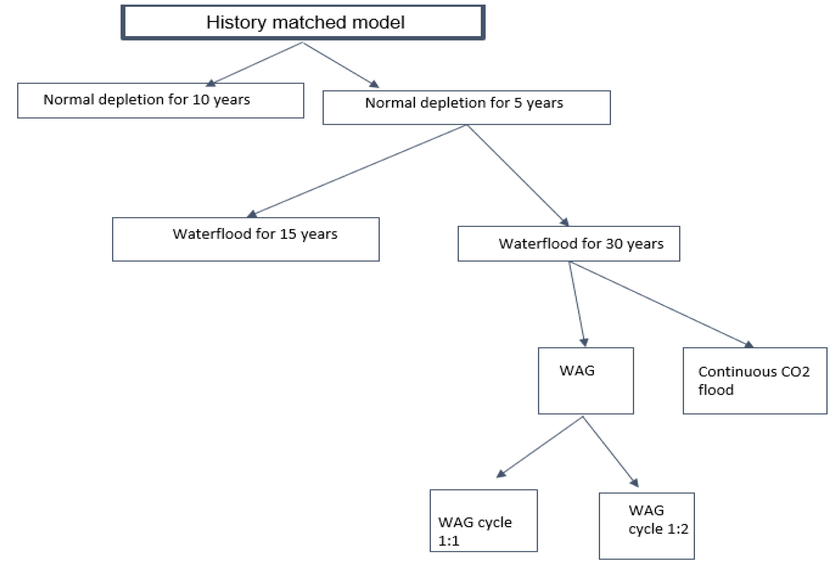
Normal Depletion for 10 years, from the history-matched model, a normal depletion (do nothing) was run for 10 years. The reservoir pressure decline was very significant and the cumulative oil production was not economical. A normal depletion for 5 years was run when the 10 years proved uneconomical with a high-pressure decline. 15-year waterflooding: This scenario was used right after the normal depletion to increase the oil recovery and increases the reservoir pressure. The reservoir pressure increased but it did not exceed the natural reservoir pressure. 30-year waterflooding: This scenario was used to increase the reservoir pressure to prepare the reservoir for CO2 flood. Continuous CO2 injection after 30-year waterflooding: In this scenario, the tertiary recovery strategy used is continuous gas (CO2) injection.
2.7. Economic Analysis
A financial feasibility study evaluated the economic performance of proposed field development plans, with net present value (NPV) serving as the key profitability metric. Production volumes (oil and gas), water injection rates, and CO2 recycling metrics were integrated into an economic forecasting framework to analyze upfront capital investments, recurring operational costs, and long-term maintenance expenditures. The largest cost drivers included ongoing operational expenses and infrastructure investments tied to the development plan’s design parameters. This financial assessment was applied across multiple tertiary recovery strategies to quantify scenario-specific economic outcomes.
2.7.1. Capital Expenditures
The capital expenditure for the CO2 recycling infrastructure encompassed critical subsystems: oil-water separation, dehydration, CO2/hydrocarbon gas separation, compression systems, H2S removal, and reinjection mechanisms for recovered CO2. Cost projections were derived from peak CO2 production rates, calculated at 15 million standard cubic feet per day (MMscf/d)—below the 30 MMscf/d threshold. Capital costs were estimated using a scaling formula tied to processing capacity, factoring in equipment, energy, and operational requirements for these integrated systems.
where CO2 Production Peak rate is represented in MMscf/d.
Capital costs for constructing processing facilities (batteries) to refine extracted oil and gas were evaluated. Facility sizing was determined by total production volumes, with peak daily processing capacity estimated at 12,000 barrels. Expenditures included fluid transport pipelines, gas gathering lines, and metering infrastructure, all incorporated into capital expenditures (CAPEX). While central and satellite battery configurations are common, this project utilized a centralized system. Design specifications required 12 storage units (1,000-barrel capacity each) to meet operational demands. The centralized battery infrastructure was projected to cost 24,000. For 12 production wells distributed across a 6.6−square−mile reservoir zone, pipeline network installation costs approximated 24,000. For 12 production wells distributed across a 6.6−square−mile reservoir zone, pipeline network installation costs approximated 3.6 million.
2.7.2. CO2 Distribution System
A financial assessment was performed to quantify expenses linked to CO2 transportation between production wells, recycling facilities, and injection sites. Project assumptions included $200,000 for manifolds and distribution pipelines. Feeder pipeline expenses—connecting compressors to manifold networks—were calculated based on two variables: injection volume and the distance between CO2 sources and target reservoirs. The total capital expenditure (CAPEX) for CO2 transport infrastructure can be modeled through a formulaic relationship accounting for these variables.
Where is the cost per mile for the selected pipe diameter. With a presumed distance of 95 miles from the CO2 source to the oil field, the selected component for the continuous CO2 flood was set at $360,000, reflecting the injected CO2 volume of 19MMscf/day. In the WAG, where the CO2 injection volume reached 31 MMscf/day, the component was estimated at $540,000. The maximum CO2 injection per day, amounting to 14.4MMscf for four injectors (WAG), maintains the component at $360,000 per mile.
2.7.3. Operating Expenditures
Maintenance costs for surface facilities included a fixed monthly baseline expenditure of 17,000 and a variable rate tied to production output, projected at 17,000 and a variable rate tied to production output, projected at 4 per barrel of oil. Water-related expenses were calculated at 0.14 per barrel and factored into net present value (NPV) assessments, with procurement volumes determined as the difference between water injection and production rates. CO2 treatment costs were modeled at 700 per million standard cubic feet (MMscf) of processed gas, integrated into financial evaluations under the assumption of full procurement of treated CO2. For simplicity, total injected CO2 volumes were equated to purchased quantities. Energy expenditures (HP) were determined through a cost−performance ratio, assuming an electricity rate of (HP) were determined through a cost−performance ratio, assuming an electricity rate of 0.15 per kilowatt-hour (kWh).
, $/HP
The horsepower (HP) required was computed using the relation
Where, CO2 injection volume is given in bbl /month; selecting a three-stage compressor,
s = 3; Safety factor, F = 1.1.
3. Results and Discussion
3.1. Results and Discussion from the CO2-Prophet
In order to optimize the effectiveness of waterflooding in the investigated field, six distinct case studies employing various injection modes were executed to assess different field development scenarios over a 15-year production period, as shown in Table 5 and the accompanying Figure 10. These findings, barring case 6, which exhibited a cumulative oil recovery of 0.1 million stock tank barrels (MSTB) over 15 years, indicate that both waterflooding and CO2 injections exhibit promising recovery potentials. The depicted figure reveals that case 4, utilizing a water-alternating-gas (WAG) injection strategy, demonstrates superior effectiveness in extracting substantial oil reserves from the field, as evidenced by a cumulative oil production of 63.109 million MSTB over 15 years, accompanied by an incremental oil recovery of 26.63%.
3.2. Results from the KM Scoping
The KM CO2 flood screening model field yields a detailed output that forecasts a total injection of 17 billion cubic feet (bcf) of CO2, with 8 bcf requiring purchase, highlighting a significant commitment to CO2 sourcing for enhanced oil recovery (EOR) as shown in Figure 11. The predicted EOR output stands at a notable 1.3 million stock tank barrels (mmstb), demonstrating the field’s capacity for substantial incremental oil production, while the net CO2 utilization efficiency is quantified at 6.1 million cubic feet per stock tank barrel (mcf/stb). The injectivity rates, both nominal and effective, are calculated at 0.074 hydrocarbon pore volume per year (hcpv/yr), indicating a well-calibrated injection strategy. The reservoir’s sizable hydrocarbon pore volume of over 3.96 million reservoir barrels (rb) per pattern, coupled with an original oil in place (OOIP) of approximately 2.57 million stock tank barrels (stb) per pattern, suggest am ple opportunity for oil displacement and production. Water injection needs are also substantial, with 12,880 barrels of water per day (bw/day) required for injection and an additional 2,400 bw/day projected, presumeably to maintain the reservoir pressure and maximize CO2 EOR efficiency. Financial projections are favorable, with an initial investment of 0.7 million dollars (mm$) and further investments in recycling facilities, tallying 0.9 mm$, totaling an overall expenditure of 1.6 mm$. The economic potential of the project is reinforced by a present value of 1.0 mm$ at a 10% discount rate (PV10%), indicating a profitable outlook for the CO2 EOR project in field post-tax.
The graphs provided in Figure 12 depict the production rates and cumulative production over a period of approximately 25 years. The left graph focuses on oil rates, showcasing three scenarios: the base case without CO2 flood (black squares), the case with CO2 flooding (green diamonds), and the cumulative oil produced due to CO2 injection (yellow triangles). The CO2 flood scenario demonstrates a noticeable increase in the oil rate compared to the base case, suggesting that CO2 injection significantly enhances oil recovery. The oil production rate remains relatively stable over the years, water production exhibits a gradual decline, and gas production appears to fluctuate slightly but remains consistent, indicating a stable gas-oil ratio (GOR). These data imply a well-managed field with a successful CO2 EOR project that stabilizes oil production rates while effectively managing water and gas production.
3.3. Simulation Results for the History Match
The precision of the match across all wells signifies a model that not only captures the complexities of the observed data but also mirrors the actual behaviors of the reservoir overtime. This alignment between the modeled and historical data underscores the model’s predictive strength and ensures confidence in its use for forecasting. The figures a synchronization of the simulated and actual data points, pointing to an exceptional match for oil, gas, and water production rates. Such a level of accuracy suggests that the model is fine tuned to the reservoir’s characteristics and dynamics. The ability of the model to reflect the precise production trends are critical for effective forecast planning. It means that the model can be trusted to predict future production scenarios with a high degree of reliability. This match also lays a solids groundwork for optimizing future reservoir exploitation strategies. The detailed match indicates a comprehensive understanding of the reservoir, which is essential for making informed decisions regarding well interventions, the implementation of enhanced oil recovery techniques, and the management of reservoir production over time. The match obtained for the water production rate is good and with such a reliable history match as a starting point, the forecast can accurately predict the timing and impact of water production allowing for the design and execution of preemptive strategies to maintain optimal oil production rates. This sets the stage for confident forecasting and strategic planning, ensuring that reservoir management can continue to maximize hydrocarbon recovery while mitigating risks and navigating the operational and economic complexities inherent in the lifecycle of the reservoir. Figure 13, Figure 14, Figure 15, Figure 16 and Figure 17 indicates the results of the history match.
3.4. Scenario 1. Development Strategy Comparison- 3 injectors/ 3 producers
Figure 18 shows a plot of the reservoir pressure over a period of 51 years. The graph begins with a steep decline in field pressure from 2000 to 2009, which is the primary recovery. This phase corresponds to the primary recovery period where oil extraction occurs naturally without external pressure support, leading to a significant drop in pressure. After the primary recovery, if no action is taken, the pressure in the field remains stable but low, approximately leveling off for 5 years. A waterflood for 15 years’ increases the reservoir pressure but this is not enough to ensure effective mixing of CO2 with the reservoir fluid in the case of the CO2 tertiary recovery. The MMP is 4100 psi therefore additional 15 years waterflood which raises the reservoir pressure to about 4300 psi makes the reservoir suitable for various tertiary mechanisms such as continuous CO2 flood and WAG.
The fracture pressure was considered in running all these scenarios, calculated as 0.9 × 0.78 × 7835, which equals 5500 psi. In Case 1 (Normal Depletion – Do Nothing), the reservoir pressure after 10 years was 1053 psi. For Case 2 (Normal Depletion), after 5 years the pressure was 1783 psi. In Case 3 (Waterflooding), the pressure increased to 2359.8 psi after 15 years, and in Case 4 (Waterflooding over 30 years), it rose further to 4195.4 psi. Case 5 (WAG 1:1) resulted in a pressure of 4887 psi after 10 years, while Case 6 (WAG 1:1 over 6 years) gave a pressure of 4598.7 psi. In Case 7 (WAG 1:2), the reservoir pressure reached 5366 psi after 10 years, approaching the fracture pressure, and in Case 8 (WAG 1:2 over 6 years), it was 4865.5 psi. For Case 9 (Continuous CO₂ Injection), the pressure was 4546 psi after 10 years, and in Case 10 (Continuous CO₂ Injection over 6 years), it was 4306.8 psi. All simulated pressures remained below the fracture pressure of 5500 psi, indicating that the reservoir integrity was maintained under these management scenarios within the given time frames.
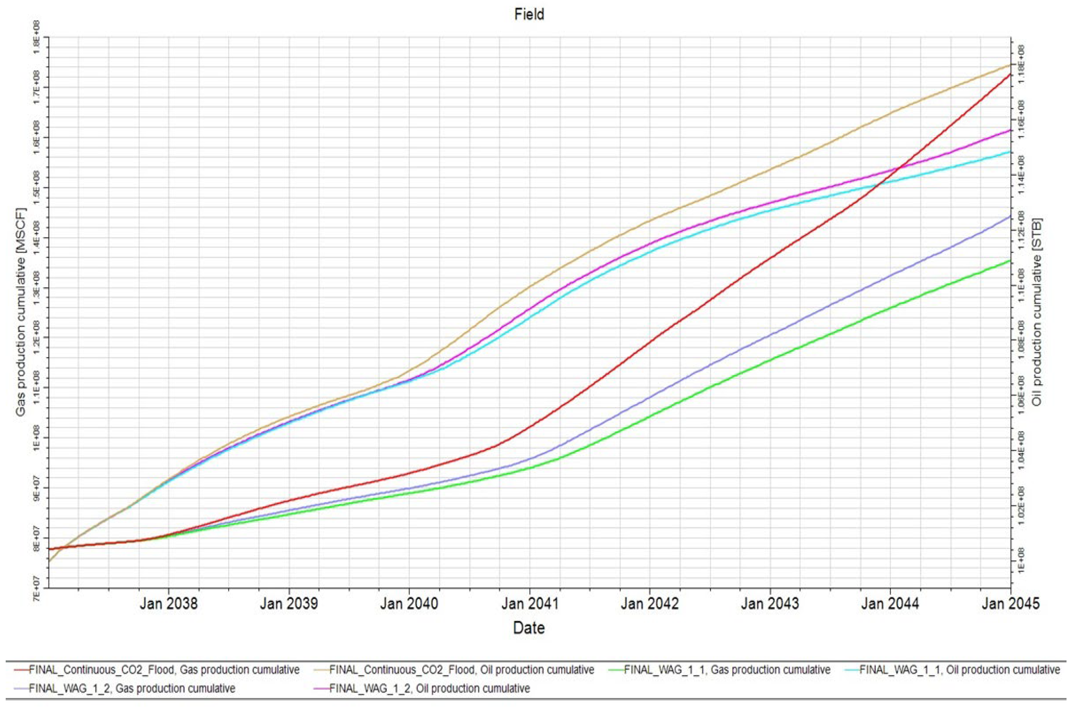
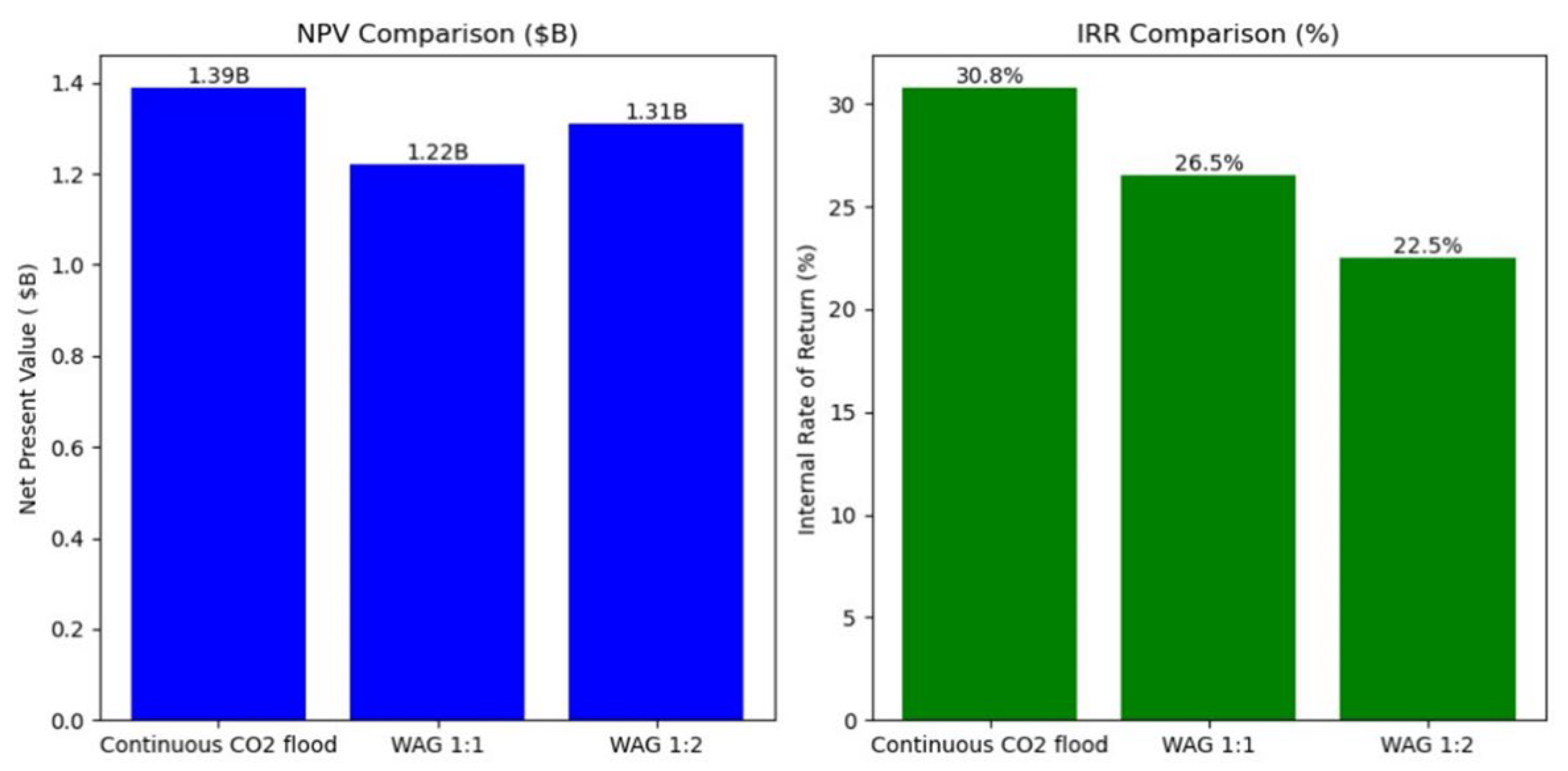
Figure 19 illustrates the trends of reservoir pressure, oil production, and gas production over time during the primary and natural depletion phases. It is observed that both oil and gas production rates, along with reservoir pressures, diminish progressively during these phases. Notably, gas production remains consistently higher throughout the period, although the disparity between the production rates of oil and gas is relatively small. During primary depletion, oil production gradually declined from approximately 7200 STB/d to 2000 STB/d, while gas production decreased from 5510 MSCF/d to 2800 MSCF/d. In the natural depletion phase, the oil production further reduced to 1800 STB/d, and the gas production dropped to 1500 MSCF/d. Figure 20 extends the analysis from Figure 19, displaying a gradual increase in the reservoir pressure following the initiation of water injection, which stabilizes at around 4300 psi after 30 years. Concurrently, there is an initial resurgence in oil production at the start of waterflooding; however, this production peak is transient, and a gradual decline ensues until stabilization at 1200 STB/day. At this juncture, the elevated reservoir pressure facilitates effective CO2 mixing for enhanced oil recovery (EOR) applications. Figure 21 delineates the enhancement in oil production following the implementation of water-alternating gas (WAG) cycles at ratios of 1:1 and 2:2, and continuous CO2 injection strategies. Figure 25 compares cumulative oil and gas production across various development scenarios, highlighting that continuous CO2 injection yields the highest outputs, followed by the WAG cycle at a ratio of 1:2, and subsequently by the WAG cycle at a ratio of 1:1.
Figure 23.
Cumulative oil and gas production for waterflooding.
Figure 24 presents the oil saturation maps following the 30-year period of waterflooding. The observed oil saturation values ranged from 0.5 to 0.8, indicating a significant quantity of recoverable oil remaining within the reservoir.
3.5. Scenario 2. Development Strategy Comparison- Infill Wells (Five-spot inverted)
In this scenario, 12 more wells were drilled using the five-spot inverted pattern. 12 producers and 6 injectors. Figure 26 shows the streamlines describing interconnectivity between the producers and injectors.
Figure 27 illustrates the comparison of the various development cases in this scenario. Similar to scenario 1, pressure and oil production decline for both the primary and normal depletion. Oil Production increases steeply at the start of the water flood but gradually reduces as the pressure keeps increasing for the 30-year period.
Figure 29.
cumulative Oil and Gas production for all tertiary recovery scenarios.
4. Economic Analysis – Scenario 1, 3 Injectors/ 3 Producers
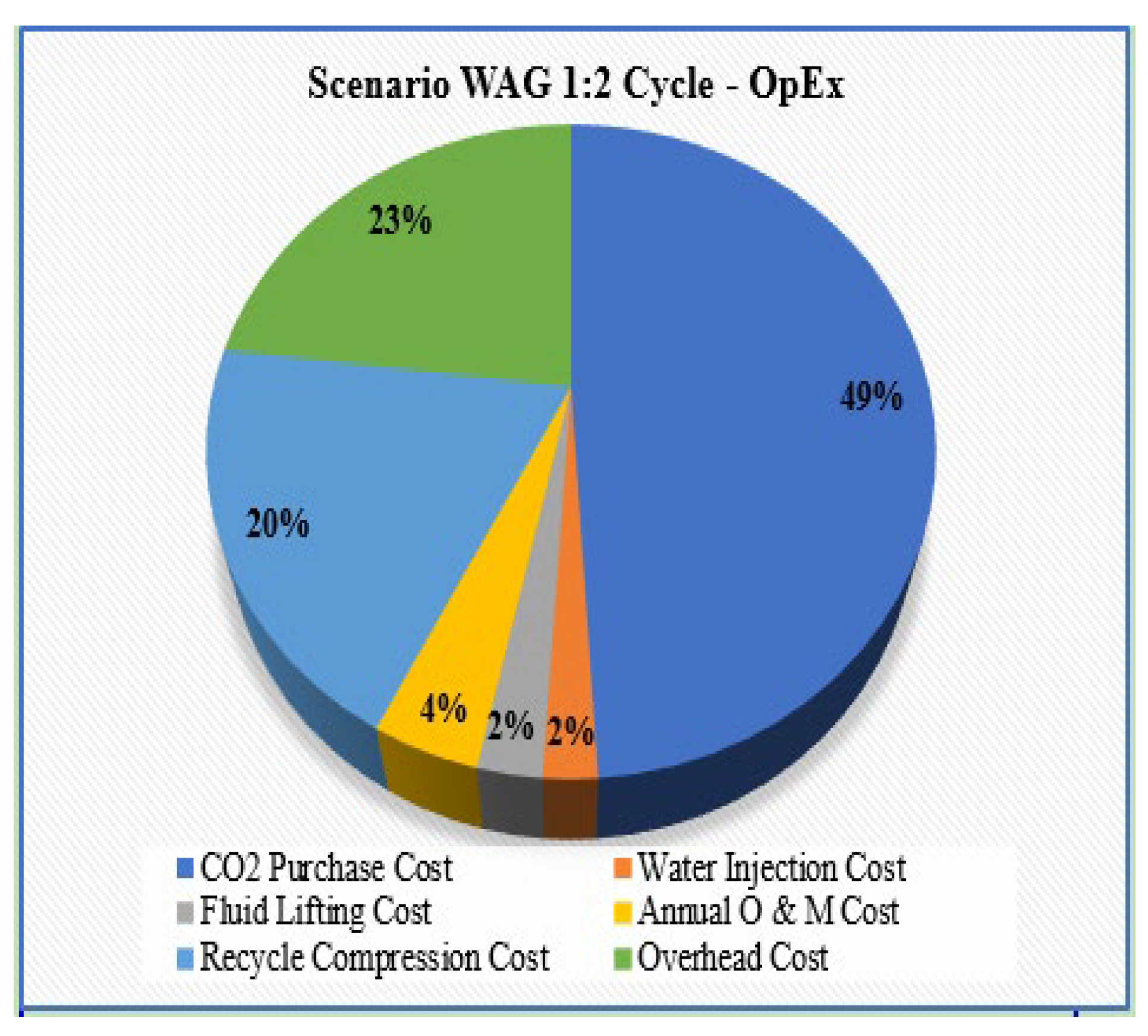
Table 6, Table 8 and Table 10 outlines the capital expenditure (CAPEX) details for the continuous CO2 injection, WAG cycle 1:1 and WAG cycle 1:2 cases in a reservoir management project. Its itemizes the costs associated with the different components essential for the implementation of the CO2 injection. Table 7, Table 9 and Table 11 provides a detailed breakdown of the annual operat ing expenses (OPEX) for the same cases.
Table 4.
Capex for continuous CO2.
|
CAPEX – Continuous CO2 scenario |
|
| Converting to CO2 Wells | $ 1,998,000 |
| C02 Supply and Distribution | $ 60,360,00 |
| Capital Cost for Compressor | $ 8,221,423 |
| Recycle Cost | $ 22,122,900 |
| Total | $ 70,519,323 |
Figure 30.
Capital Expenditure for continuous CO2 flood.
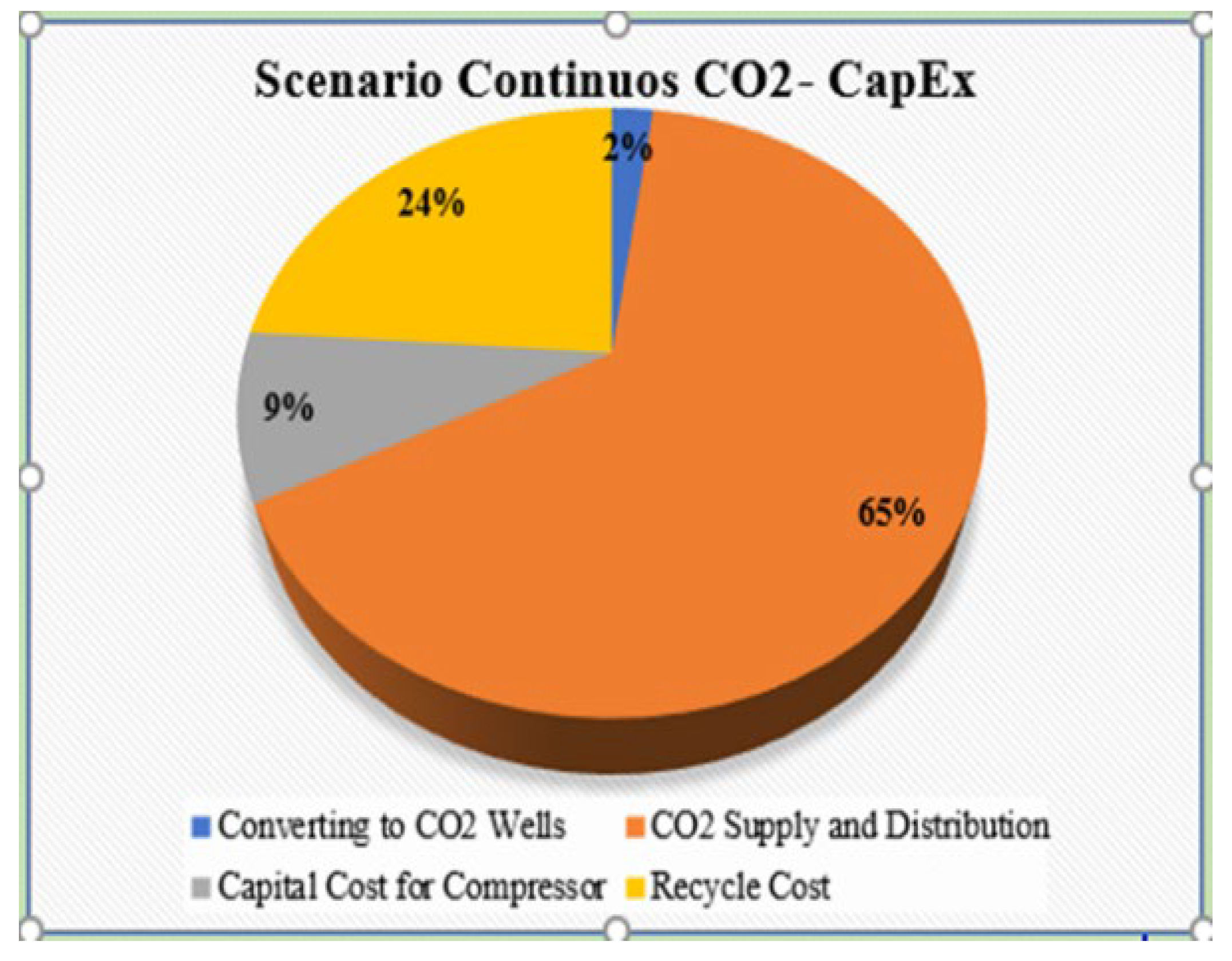
Table 5.
Operating Expenditure for Continuous CO2 flood.
| OPEX Yearly | |
| C02 Purchase Cost | $13,140,000 |
| Fluid Lifting Cost | $509,071 |
| Annual O & M Cost | $949,200 |
| CO2 Compression Cost | $2,832,811 |
| Overhead Cost | $5,229, 427.26 |
| Total | $22,660,853 |
Figure 31.
Operating Expenditure for CO2 flood.
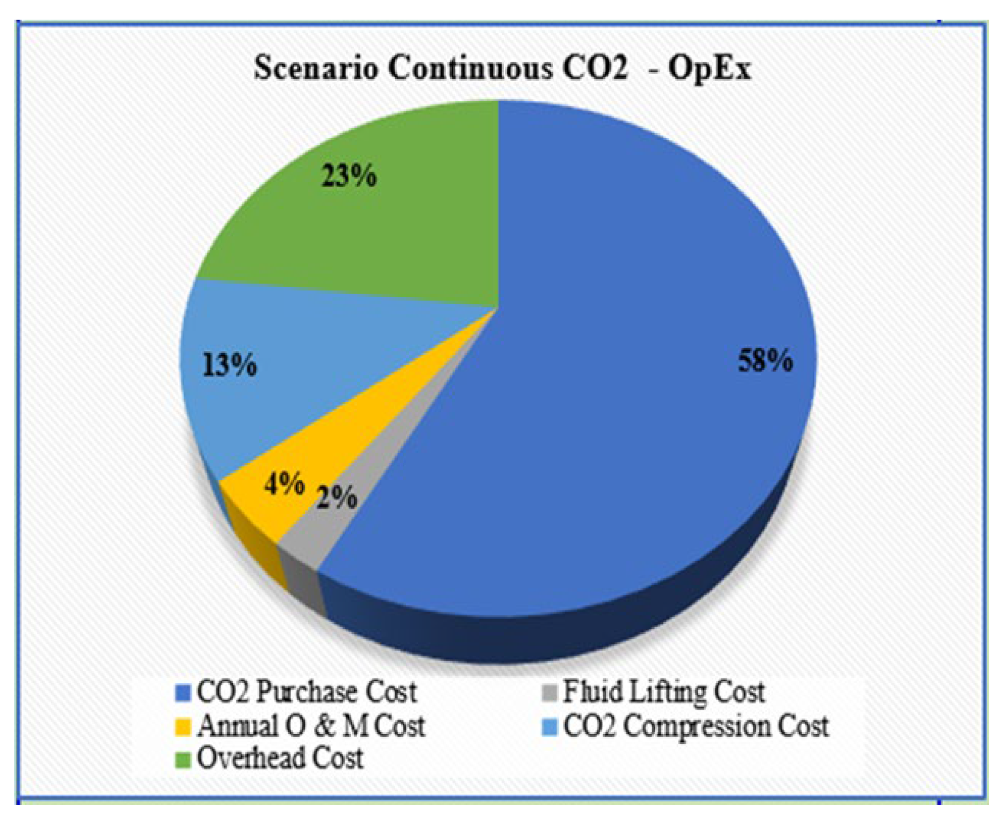
Table 6.
Capital Expenditure for WAG 1:1 Cycle.
| CAPEX Yearly | |
| Converting to C02 wells | $1,998,000.00 |
| CO2 Supply and Distribution | $55,360,000.00 |
| Recycle Cost | $10,529,000.00 |
| CO2 Compression Cost | $8,330,000.00 |
| Water Treatment System | $5,229, 427.26 |
| Total | $68,988,000.00 |
Figure 32.
Capital Cost for WAG 1:1.
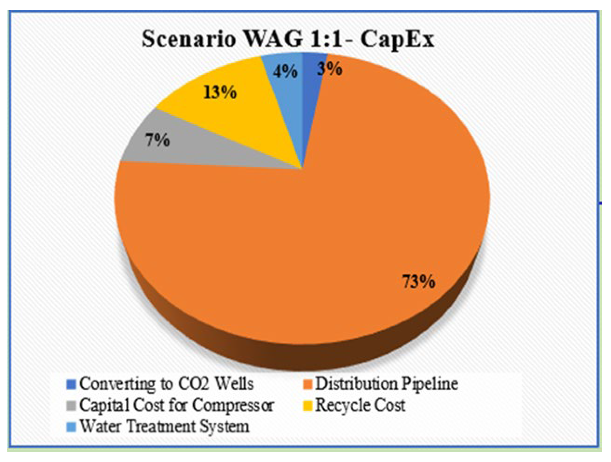
Table 7.
Operating cost for WAG 1:1.
| OPEX Yearly | |
| CO2 Purchase Cost | $8,140,000.00 |
| Water Injection Cost | $395,657.00 |
| Fluid Lifting Cost | $488,698.00 |
| Annual O & M Cost | $949,200.00 |
| Recycle Compression Cost | $4,832,980.00 |
| Overhead Cost | 4,441,960.50 |
| Total | $19,248,496.0 |
Figure 33.
Opex for WAG 1:1.
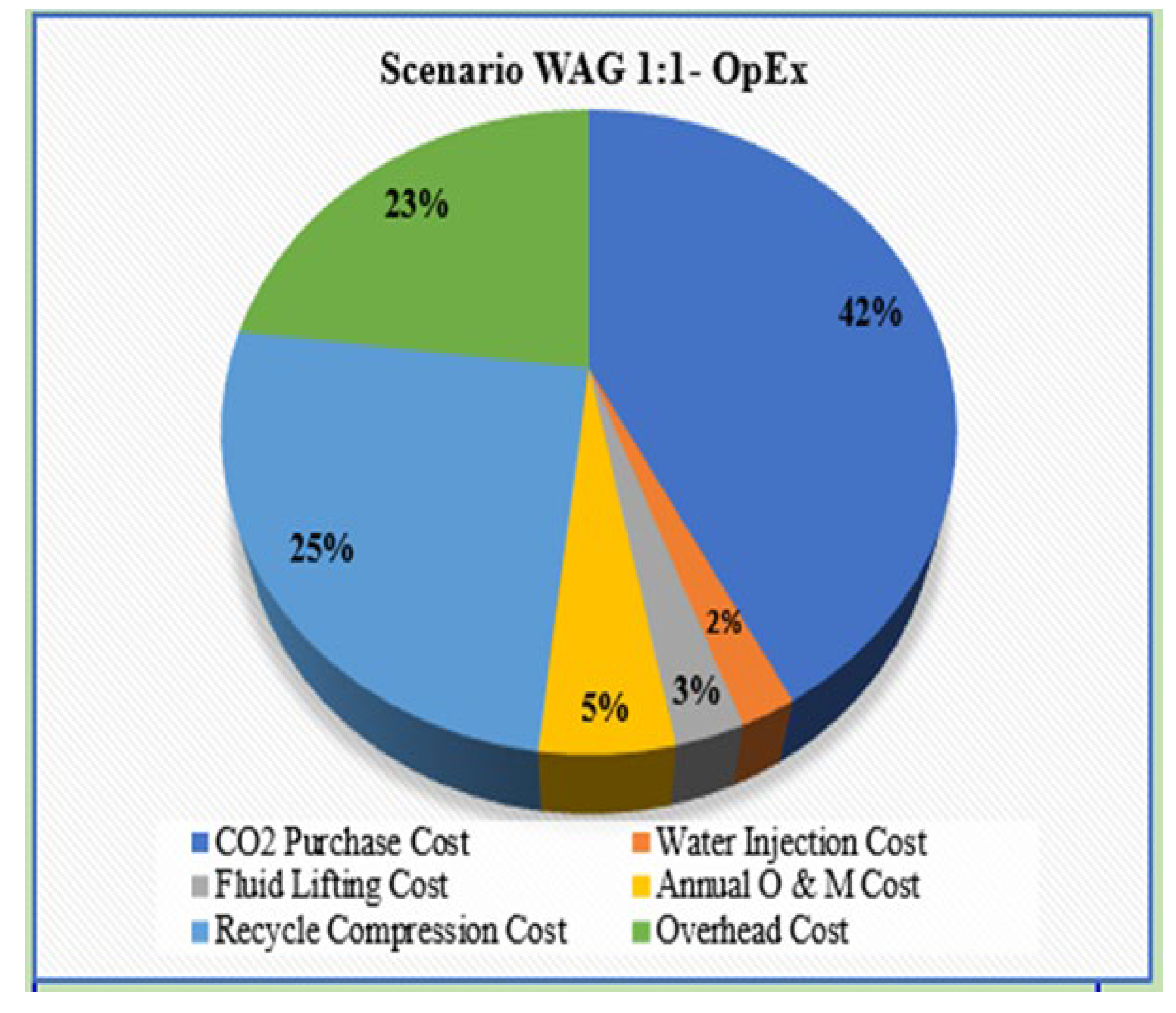
Table 8.
Capex for WAG 1:2.
| CAPEX Yearly | |
| Converting to CO2 Wells | $1,998,000.00 |
| CO2 Supply and Distribution | $55,360,000.00 |
| Capital Cost for Compressor | $8,330,000.00 |
| Recycle Cost | $10,529,000.00 |
| Water Treatment System | $3,300,000.00 |
| Total | $68,988,000.00 |
Figure 34.
Capex for WAG 1:2.
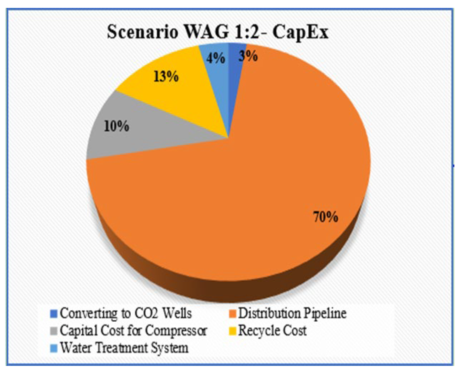
Table 9.
Opex for WAG 1:2.
| OPEX Yearly | |
| CO2 Purchase Cost | $10,140,000.00 |
| Water Injection Cost | $395,657.00 |
| Fluid Lifting Cost | $508,698.00 |
| Annual O & M Cost | $949,200.00 |
| Recycle Compression Cost | $4,832,980.00 |
| Overhead Cost | 5,047,960.50 |
| Total | $21,874,496.00 |
Figure 35.
Opex for WAG 1:2.

Figure 36.
NPV/IRR Comparisons.
4.1. Economic Analysis – Scenario 2, 12 Injectors / 6 Producers
Table 12, Table 14 and Table 16 outlines the capital expenditure (CAPEX) details for the continuous CO2 injection, WAG cycle 1:1 and WAG cycle 1:2 cases in a reservoir management project. It itemizes the costs associated with the different components essential for the implementation of the CO2 injection. Table 13, Table 15 and Table 17 provides a detailed breakdown of the annual operating expenses (OPEX) for the same cases.
Table 10.
Capex for continuous CO2.
| CAPEX – Continuous CO2 | scenario |
| Drilling of Infill Wells | $ 72,000,000.00 |
| C02 Supply and Distribution | $ 60,360,000.00 |
| Capital Cost for Compressor | $ 8,330,000.00 |
| Converting to CO2 wells | $ 4,050,000.00 |
| Recycle Cost | 22,125,000.00 |
| Total | $ 162,815,000.00 |
Figure 37.
Capex for Continuous CO2.
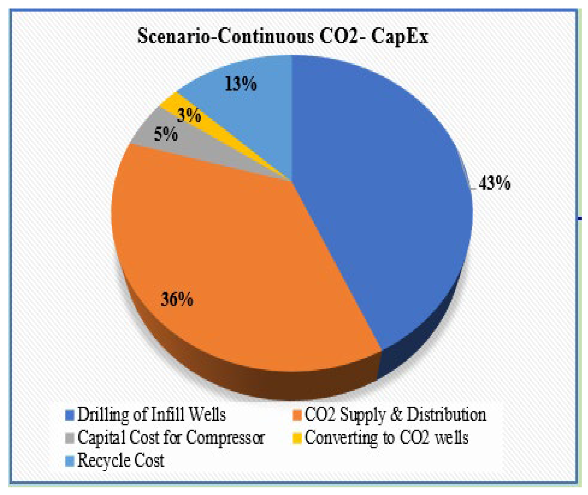
Table 11.
Opex for Continuous CO2.
| OPEX Yearly | |
| CO2 Purchase Cost | $15,140,000.00 |
| Water Injection Cost | $395,657.00 |
| Fluid Lifting Cost | $708,698.00 |
| Annual O & M Cost | $989,200.00 |
| Recycle Compression Cost | $4,832,980.00 |
| Overhead Cost | $6,501,263.40 |
| Total | $28,172,141.00 |
Figure 38.
Opex for continuous CO2.
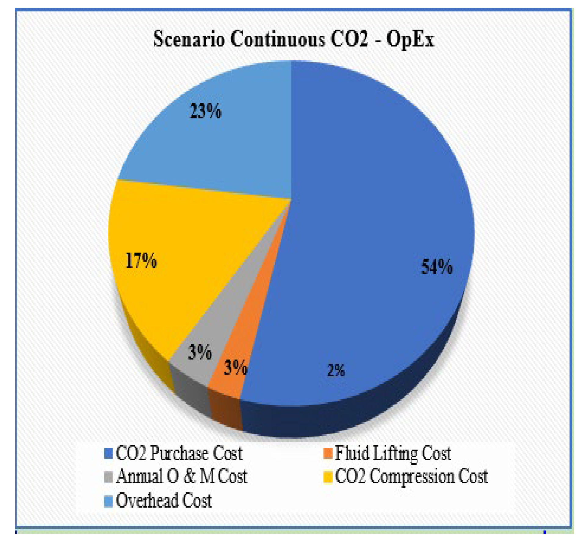
Table 12.
Capex for WAG 1:1.
| CAPEX – WAG | scenario |
| Drilling of Infill Wells | $ 72,000,000.00 |
| C02 Supply and Distribution | $ 55,360,000.00 |
| Capital Cost for Compressor | $ 8,330,000.00 |
| Converting to CO2 wells | $ 4,050,000.00 |
| Recycle Cost | 22,125,000.00 |
| Total | $ 146,219,000.00 |
Figure 39.
Capex for WAG 1:1.
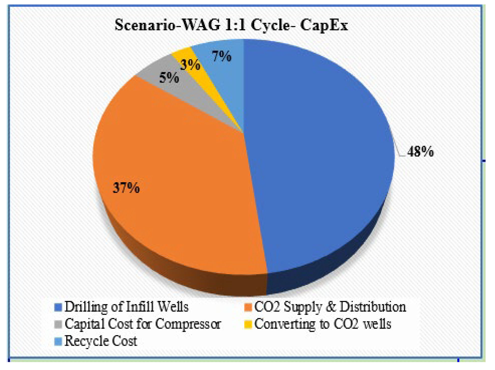
Table 13.
Opex for WAG 1:1.
| OPEX Yearly | |
| CO2 Purchase Cost | $10,140,000.00 |
| Water Injection Cost | $495,657.00 |
| Fluid Lifting Cost | $588,698.00 |
| Annual O & M Cost | $989,200.00 |
| Recycle Compression Cost | $4,832,980.00 |
| Overhead Cost | $5,113,960.50 |
| Total | $22,160,496.00 |
Figure 40.
Opex for WAG 1:1.
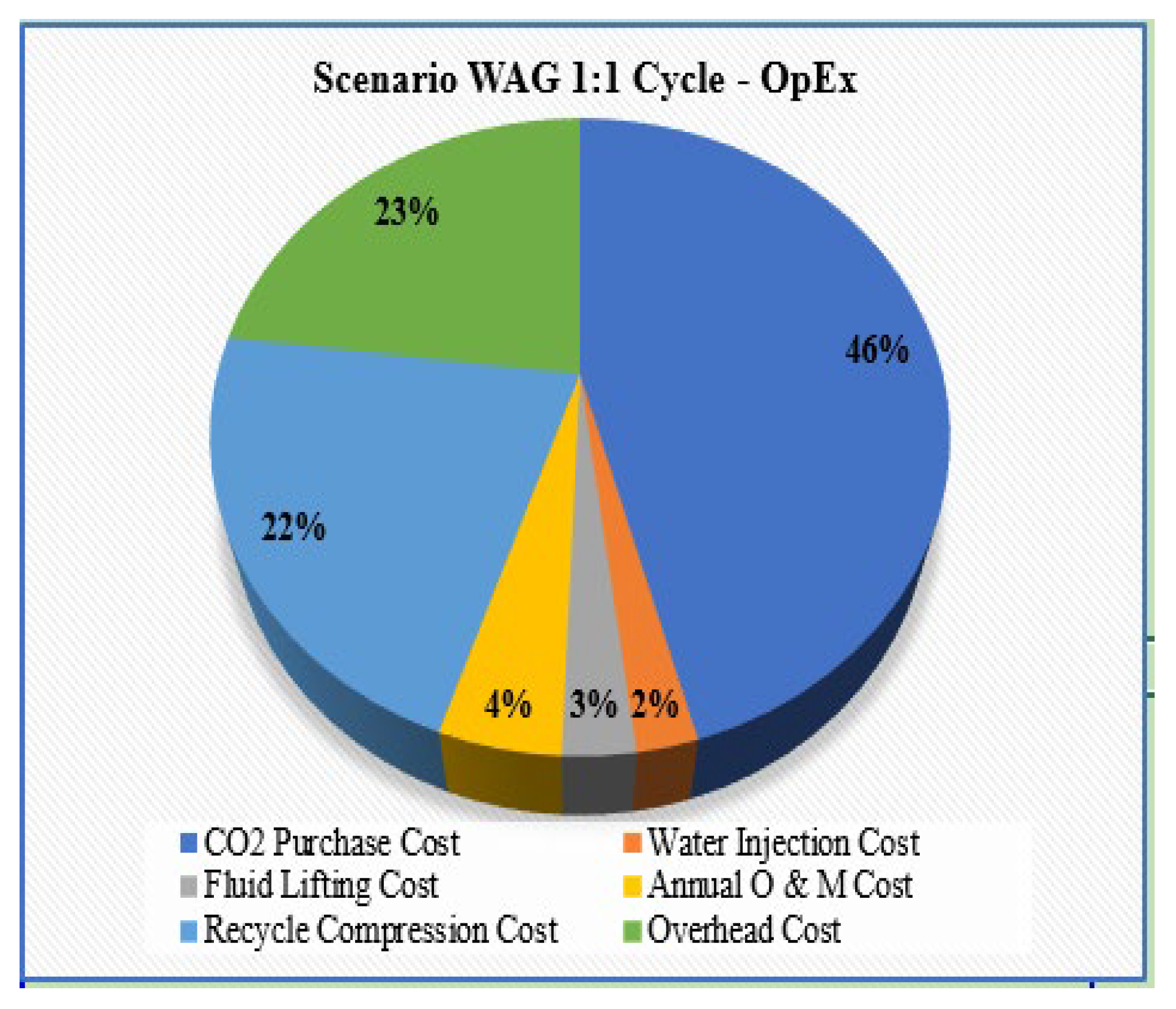
Table 14.
Capex for WAG 1:2.
| CAPEX – WAG | scenario |
| Drilling of Infill Wells | $ 72,000,000.00 |
| C02 Supply and Distribution | $ 55,360,000.00 |
| Capital Cost for Compressor | $ 8,330,000.00 |
| Converting to CO2 wells | $ 4,050,000.00 |
| Water treatment system | $ 3,800,000.00 |
| Recycle Cost | 22,125,000.00 |
| Total | $ 157,815,000.00 |
Figure 41.
Capex for WAG 1:2.
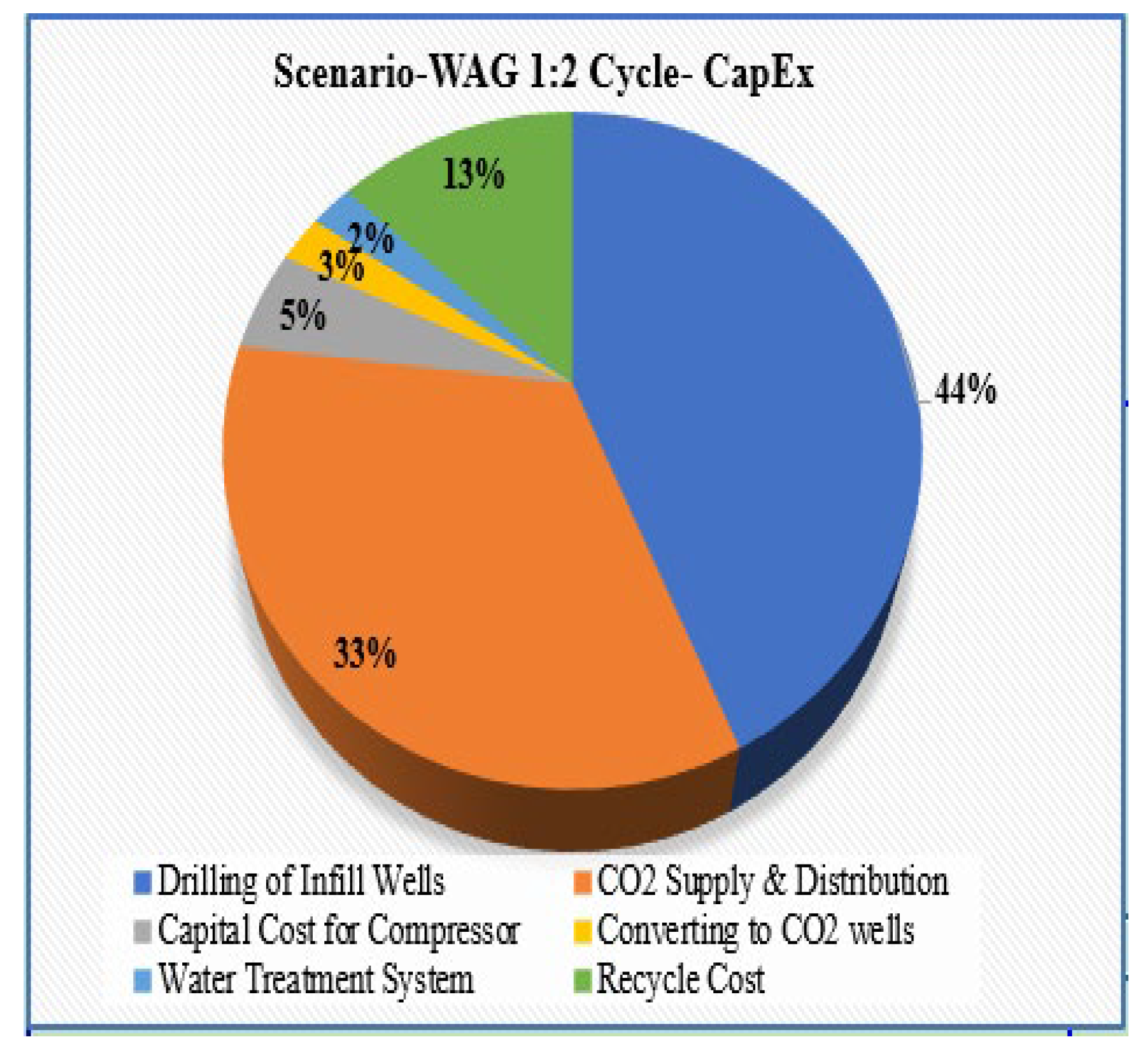
Table 15.
Opex for WAG 1:2.
| OPEX Yearly | |
| CO2 Purchase Cost | $12,140,000.00 |
| Water Injection Cost | $495,657.00 |
| Fluid Lifting Cost | $588,698.00 |
| Annual O & M Cost | $989,200.00 |
| Recycle Compression Cost | $4,832,980.00 |
| Overhead Cost | $5,713,960.50 |
| Total | $24,760,496.00 |
Figure 42.
Opex for WAG 1:2.
5. Conclusions
After employing a comprehensive array of screening techniques, geologically heterogeneous reservoir field was identified as a prime candidate for CO2 Enhanced Oil Recovery (EOR). This assessment is underpinned by the field’s significant potential to elevate the oil recovery rates, using CO2 as a miscible flood agent to improve the sweep efficiency across the reservoir. The strategic use of CO2 not only promises to enhance hydrocarbon recovery but also aims to optimize the overall operational economics of the field, turning it into a more profitable asset. The enhanced oil recovery potential is highlighted by the field’s favorable characteristics for CO2 miscibility, including reservoir pressure and temperature conditions that support efficient CO2 dissolution and displacement of oil. This strategic utilization of CO2 involves careful planning of injection patterns and management of injection rates to maximize contact with the oil-rich zones while minimizing gas override and early breakthrough. From an economic perspective, integrating CO2 EOR into geologically heterogeneous reservoir field development strategy is projected to yield a substantial increase in the ultimate recovery, thereby extending the field’s economic life and improving the return on investment. The cost implications of CO2 sourcing, injection infrastructure, and operational adjustments are offset by the anticipated uplift in oil production and the potential for carbon credits under environmental regulations. The potency of the reservoir model has been thoroughly validated through detailed history matching, demonstrating a superb alignment with actual historical production data for oil, gas, and water, as well as bottomhole pressures. This verification confirms the model’s accuracy in depicting the reservoir behavior under different production scenarios and its efficacy in simulating the CO2 flood dynamics. Consequently, this robust model forms the backbone of the predictive simulations that will guide the implementation of CO2 flooding, ensuring that the project is both technically feasible and economically viable. The integration of the CO2 EOR at geologically heterogeneous reservoir field is supported by solid technical assessments and promising economic forecasts, making it a well-substantiated strategy to maximize reservoir exploitation while adhering to modern energy and environmental standards.
Author Contributions
Conceptualization, K.O.D., N.N.Y, A.A., W.A., and K.B.; methodology, K.O.D., N.N.Y., A.A., W.A., and K.B.; software, K.O.D., N.N.Y., A.A., W.A., and K.B.; validation, K.O.D., N.N.Y., A.A., W.A. and K.B.; formal analysis, K.O.D., N.N.Y., A.A., W.A., and K.B.; investigation, K.O.D., N.N.Y., A.A., W.A., and K.B.; resources, W.A.; data curation, W.A. and K.O.D; writing—original draft preparation, K.O.D, N.N.Y., A.A., W.A., and K.B.; writing—review and editing, K.O.D., N.N.Y., A.A., W.A., and K.B..; visualization, K.O.D., N.N.Y., A.A., W.A., and K.B..; supervision, W.A.; project administration, W.A.; funding acquisition, W.A. All authors have read and agreed to the published version of the manuscript
Data Availability Statement
Data will be made available upon request.
Acknowledgments
We thank the Petroleum Recovery and Research Center, New Mexico Tech, for providing support and resources. We also thank the MDPI editorial team and anonymous reviewers for their helpful comments on this article.
Conflicts of Interest
The authors declare no conflicts of interest.
References
- Perera, M.S.A.; Gamage, R.P.; Rathnaweera, T.D.; Ranathunga, A.S.; Koay, A.; Choi, X. A Review of CO2-Enhanced Oil Recovery with a Simulated Sensitivity Analysis. Energies 2016, 9, 481. [Google Scholar] [CrossRef]
- Kumar, N.; Sampaio, M.A.; Ojha, K.; Hoteit, H.; Mandal, A. Fundamental aspects, mechanisms and emerging possibilities of CO2 miscible flooding in enhanced oil recovery: A review. Fuel 2022, 330. [Google Scholar] [CrossRef]
- Poplygin, V.V.; Poplygina, I.S.; Mordvinov, V.A. Influence of Reservoir Properties on the Velocity of Water Movement from Injection to Production Well. Energies 2022, 15, 7797. [Google Scholar] [CrossRef]
- SPE_39657”.
- Morrow, “Wettability and Its Effect on Oil Recovery,” 1990.
- Yuan, S.; Han, H.; Wang, H.; Luo, J.; Wang, Q.; Lei, Z.; Xi, C.; Li, J. Research progress and potential of new enhanced oil recovery methods in oilfield development. Pet. Explor. Dev. 2024, 51, 963–980. [Google Scholar] [CrossRef]
- S. E. Greenberg, “ILLINOIS BASIN DECATUR PROJECT Final Report An Assessment of Geologic Carbon Sequestration Options in the Illinois Basin: Phase III.
- CMTC-151027-PP NETL CO 2 Injection and Storage Cost Model,” 2012.
- Bikkina, P.; Wan, J.; Kim, Y.; Kneafsey, T.J.; Tokunaga, T.K. Influence of wettability and permeability heterogeneity on miscible CO2 flooding efficiency. Fuel 2016, 166, 219–226. [Google Scholar] [CrossRef]
- Katterbauer, K.; Arango, S.; Sun, S.; Hoteit, I. Multi-data reservoir history matching for enhanced reservoir forecasting and uncertainty quantification. J. Pet. Sci. Eng. 2015, 128, 160–176. [Google Scholar] [CrossRef]
- Zhao, H.; Li, Y.; Cui, S.; Shang, G.; Reynolds, A.C.; Guo, Z.; Li, H.A. History matching and production optimization of water flooding based on a data-driven interwell numerical simulation model. J. Nat. Gas Sci. Eng. 2016, 31, 48–66. [Google Scholar] [CrossRef]
- Rwechungura, R.W.; Dadashpour, M.; Kleppe, J. Advanced History Matching Techniques Reviewed. SPE Middle East Oil and Gas Show and Conference. LOCATION OF CONFERENCE, BahrainDATE OF CONFERENCE;
- Abdullah, N.; Hasan, N. The implementation of Water Alternating (WAG) injection to obtain optimum recovery in Cornea Field, Australia. J. Pet. Explor. Prod. Technol. 2021, 11, 1475–1485. [Google Scholar] [CrossRef]
- Sadeghnejad, S.; Manteghian, M.; Ruzsaz, H. Simulation Optimization of Water Alternating Gas (WAG) Process under Operational Constraints: A Case Study in the Persian Gulf. Sci. Iran. 2019, 26, 3431–3446. [Google Scholar] [CrossRef]
- Rahimi, V.; Bidarigh, M.; Bahrami, P. Experimental Study and Performance Investigation of Miscible Water-Alternating-CO2Flooding for Enhancing Oil Recovery in the Sarvak Formation. Oil Gas Sci. Technol. – Rev. d’IFP Energies Nouv. 2017, 72, 35. [Google Scholar] [CrossRef]
- Bui, D.; Nguyen, S.; Ampomah, W.; Acheampong, S.A.; Hama, A.; Amosu, A.; Koray, A.-M.; Kubi, E.A. A Comparison of Water Flooding and CO2-EOR Strategies for the Optimization of Oil Recovery: A Case Study of a Highly Heterogeneous Sandstone Formation. Gases 2024, 5, 1. [Google Scholar] [CrossRef]
- J. A. Mou, “A PROJECT PROPOSAL On ‘“Simulation on oil production from steam flooding process in heavy oil-sand reservoirs.
- Wang, L.; Tian, Y.; Yu, X.; Wang, C.; Yao, B.; Wang, S.; Winterfeld, P.H.; Wang, X.; Yang, Z.; Wang, Y.; et al. Advances in improved/enhanced oil recovery technologies for tight and shale reservoirs. Fuel 2017, 210, 425–445. [Google Scholar] [CrossRef]
- A Almehaideb, R.; Al-Khanbashi, A.S.; Abdulkarim, M.; A Ali, M. EOS tuning to model full field crude oil properties using multiple well fluid PVT analysis. J. Pet. Sci. Eng. 2000, 26, 291–300. [Google Scholar] [CrossRef]
- Gunda, D.; Ampomah, W.; Grigg, R.; Balch, R. Reservoir Fluid Characterization for Miscible Enhanced Oil Recovery. Carbon Management Technology Conference. LOCATION OF CONFERENCE, United StatesDATE OF CONFERENCE;
Figure 1.
Well logs showing the reservoir geology.
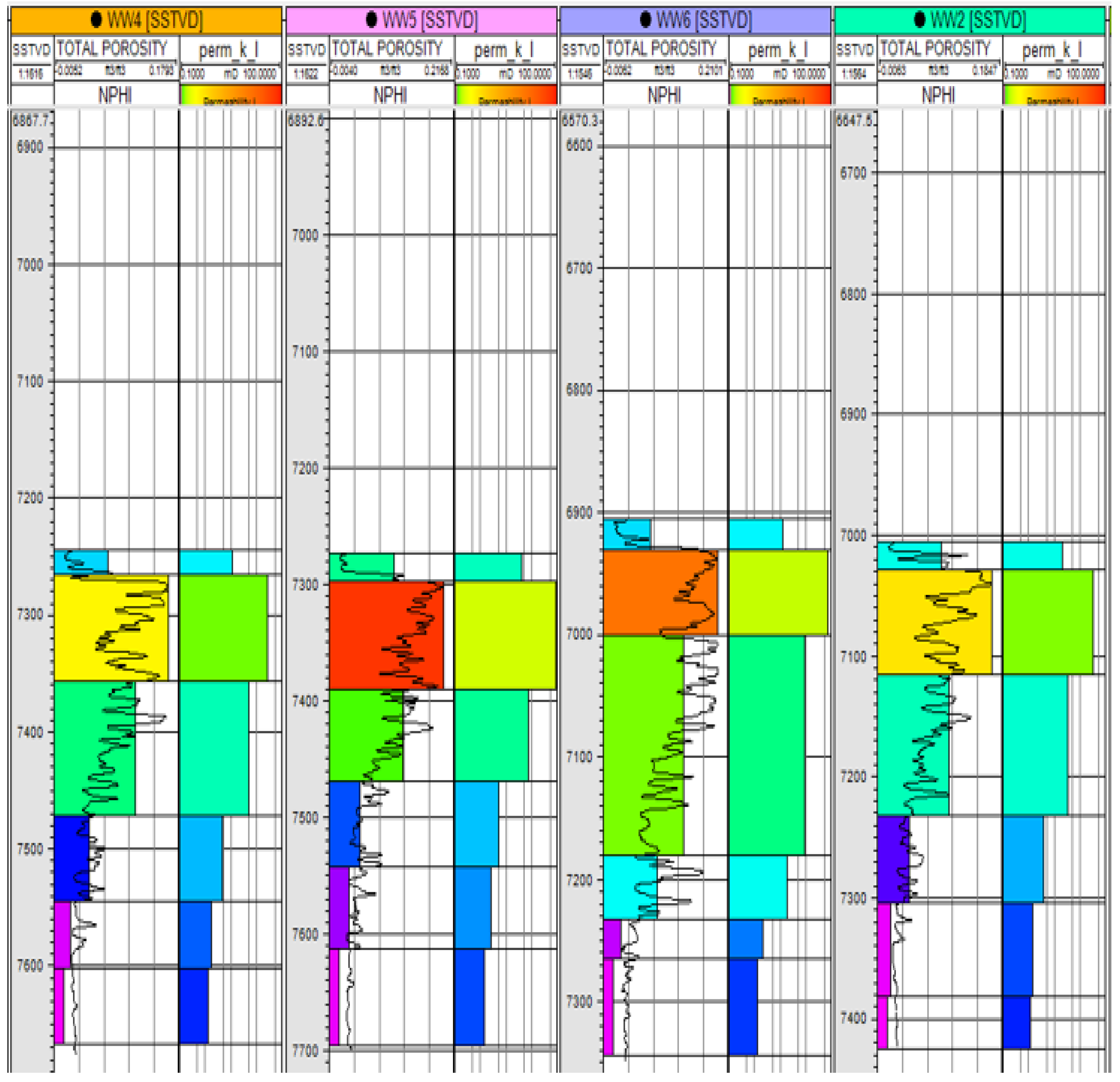
Figure 2.
Image of the Geological Model.
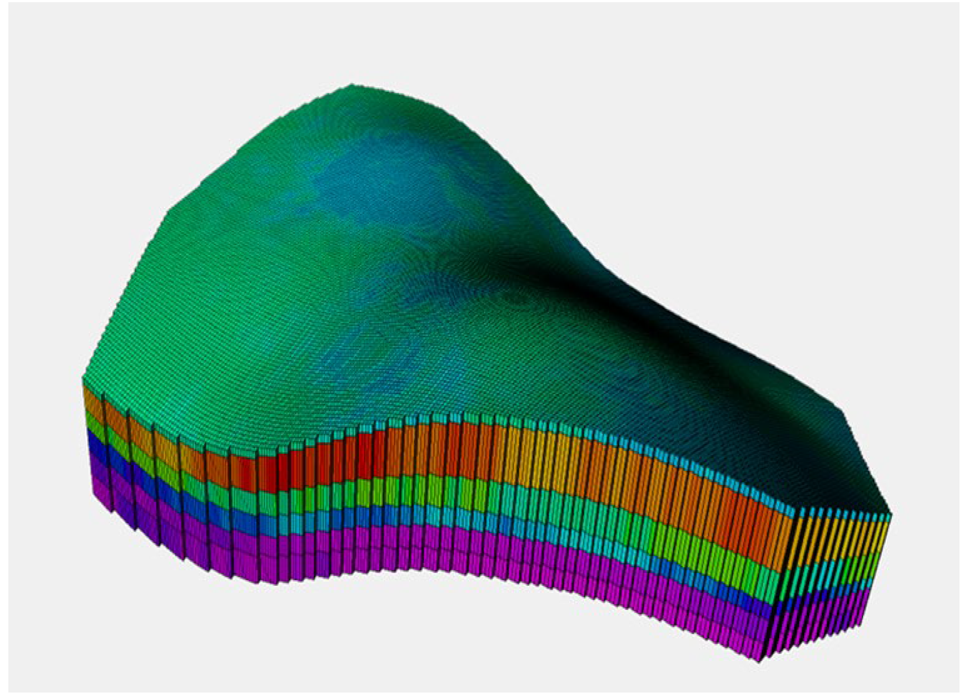
Figure 3.
3D porosity distribution of the Field for the Upscaled model.
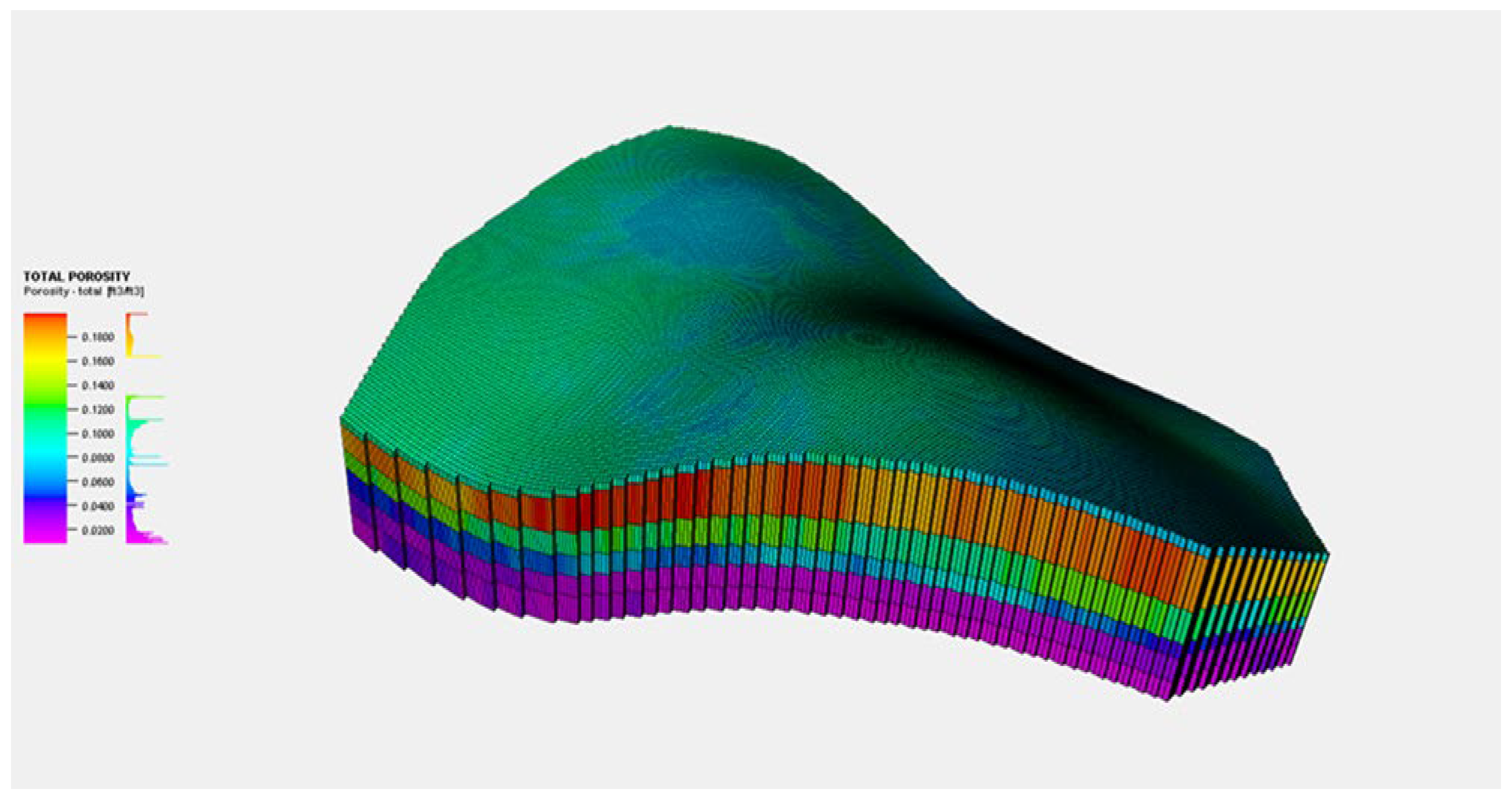
Figure 4.
3D permeability distribution of the field for Upscaled model.
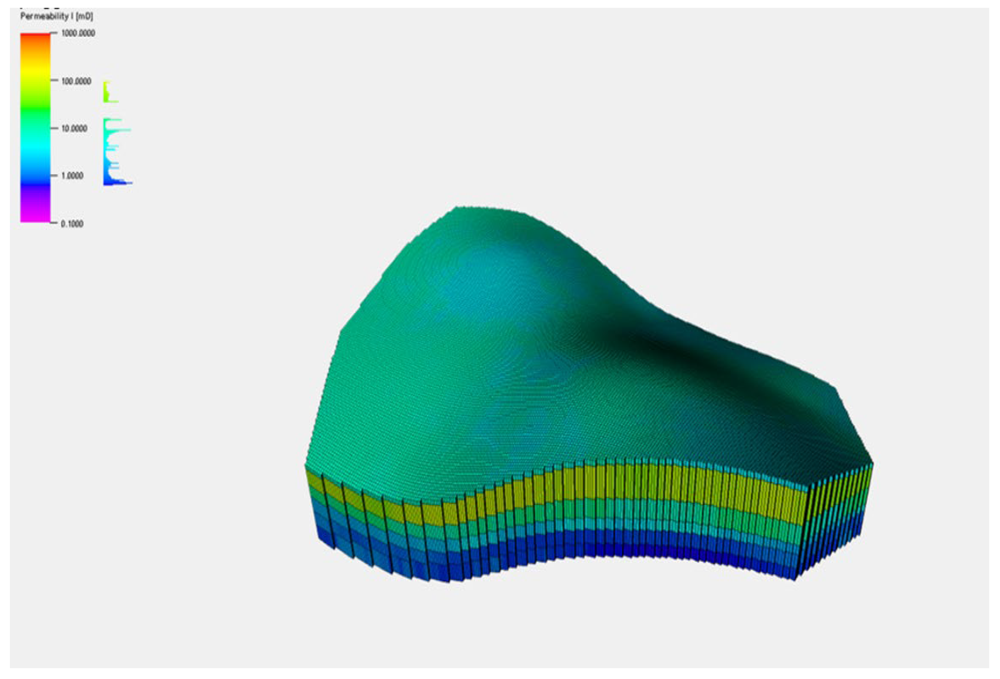
Figure 5.
Input data for the KM scoping model.
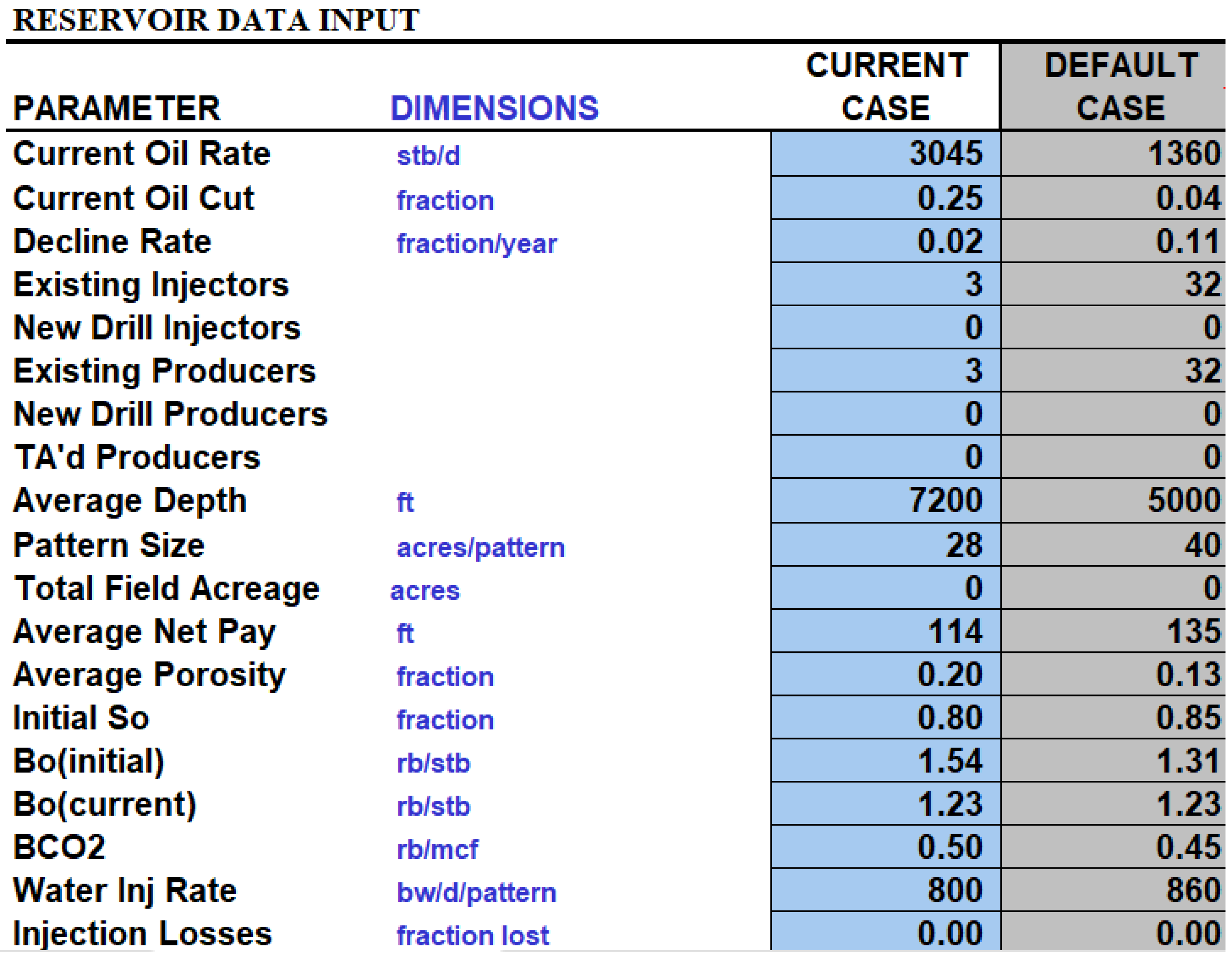
Figure 6.
Phase envelope for the fluid Model at reservoir condition 220oF.
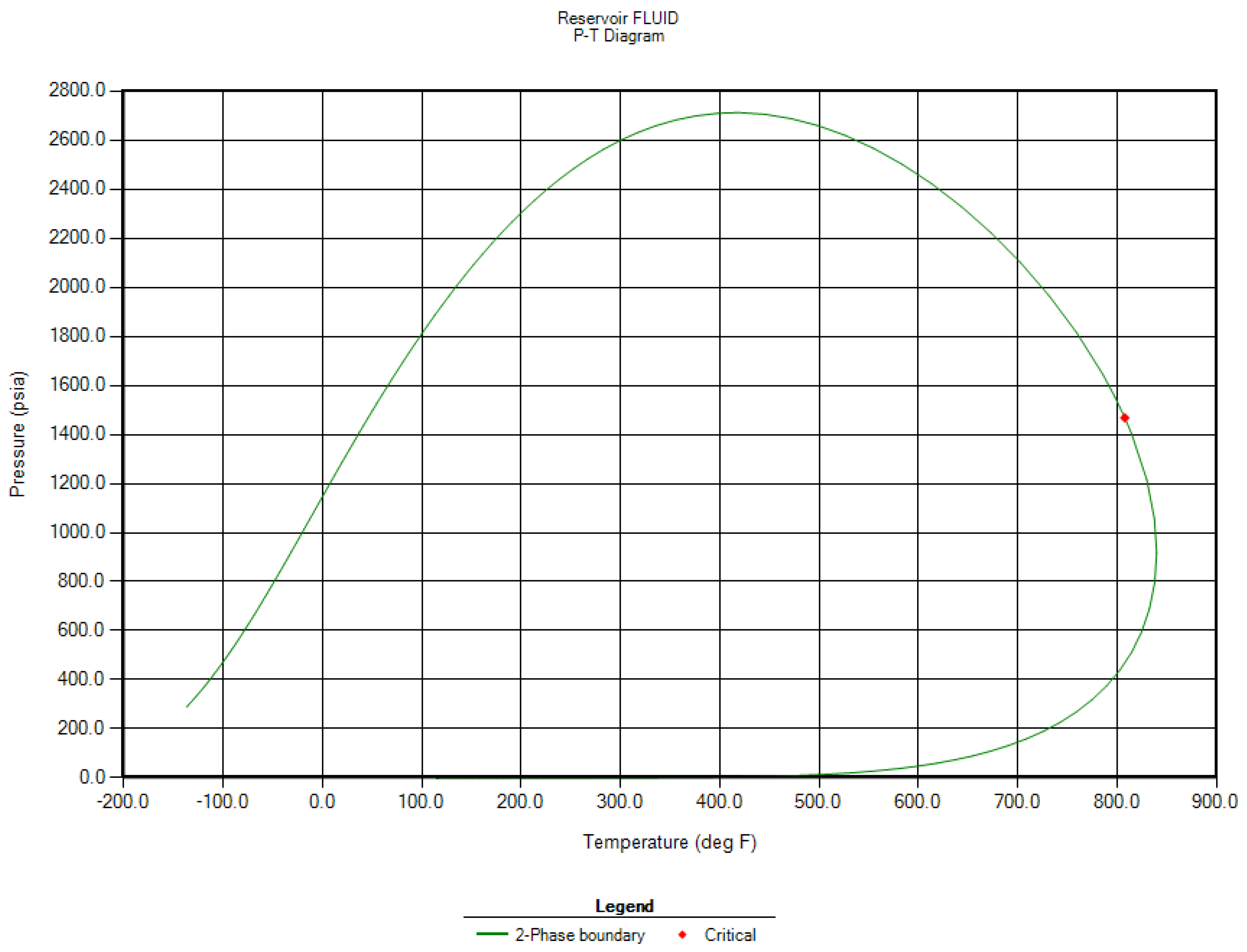
Figure 7.
Water –oil relative permeability curves used in history match.
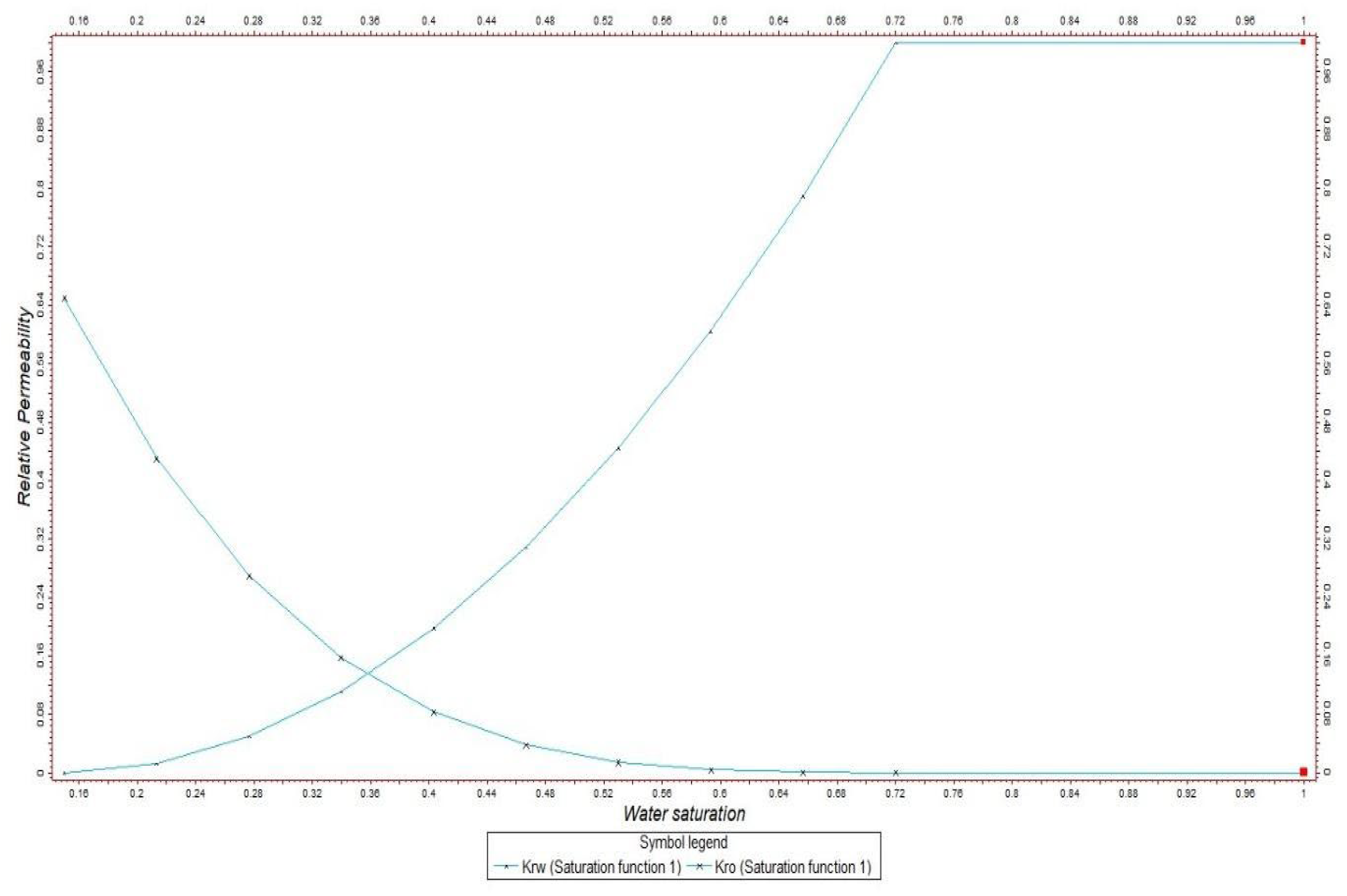
Figure 8.
Oil-gas relative permeability curves used in history match.
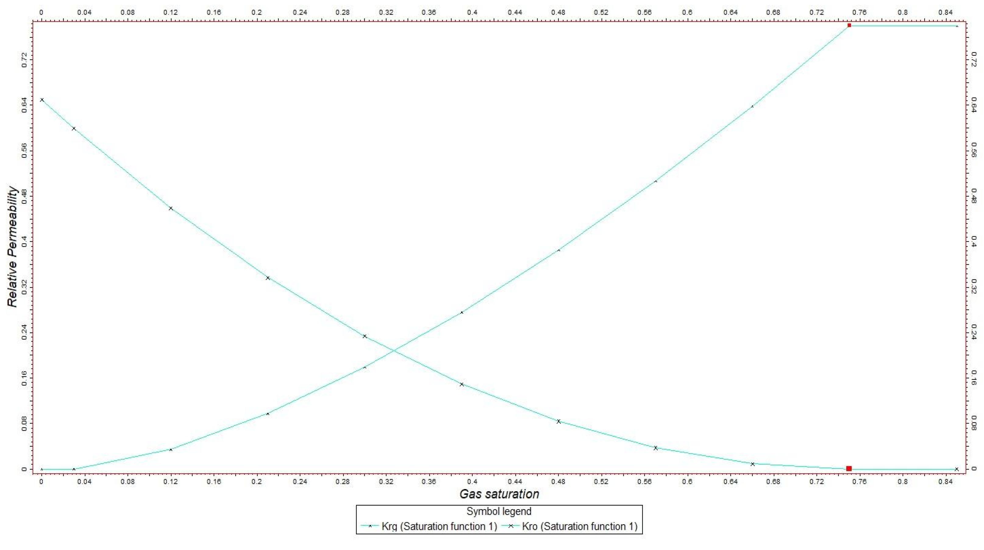
Figure 10.
Cumulative oil production for all cases.
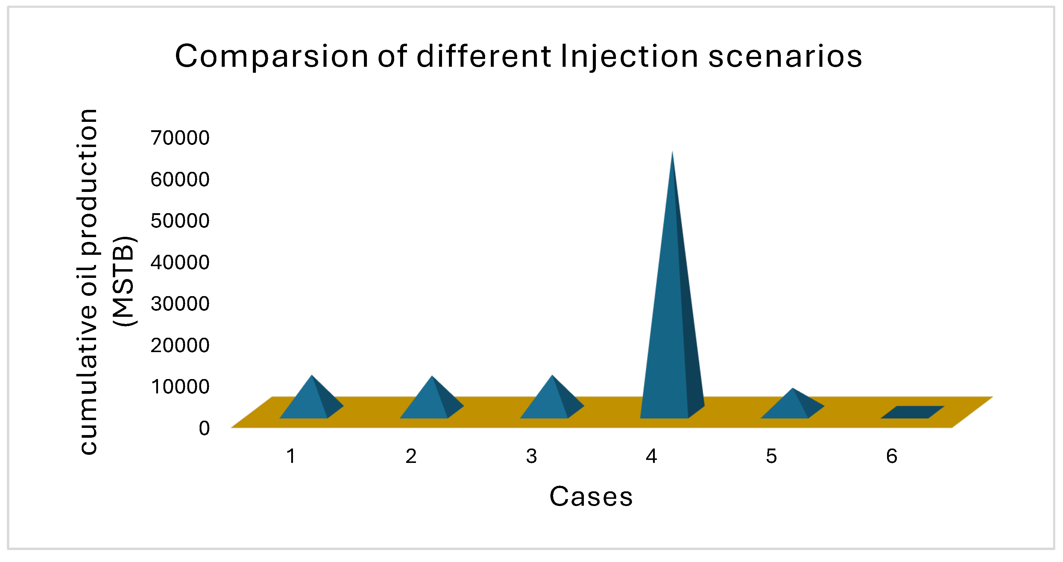
Figure 11.
Output results from the KM scoping simulation.
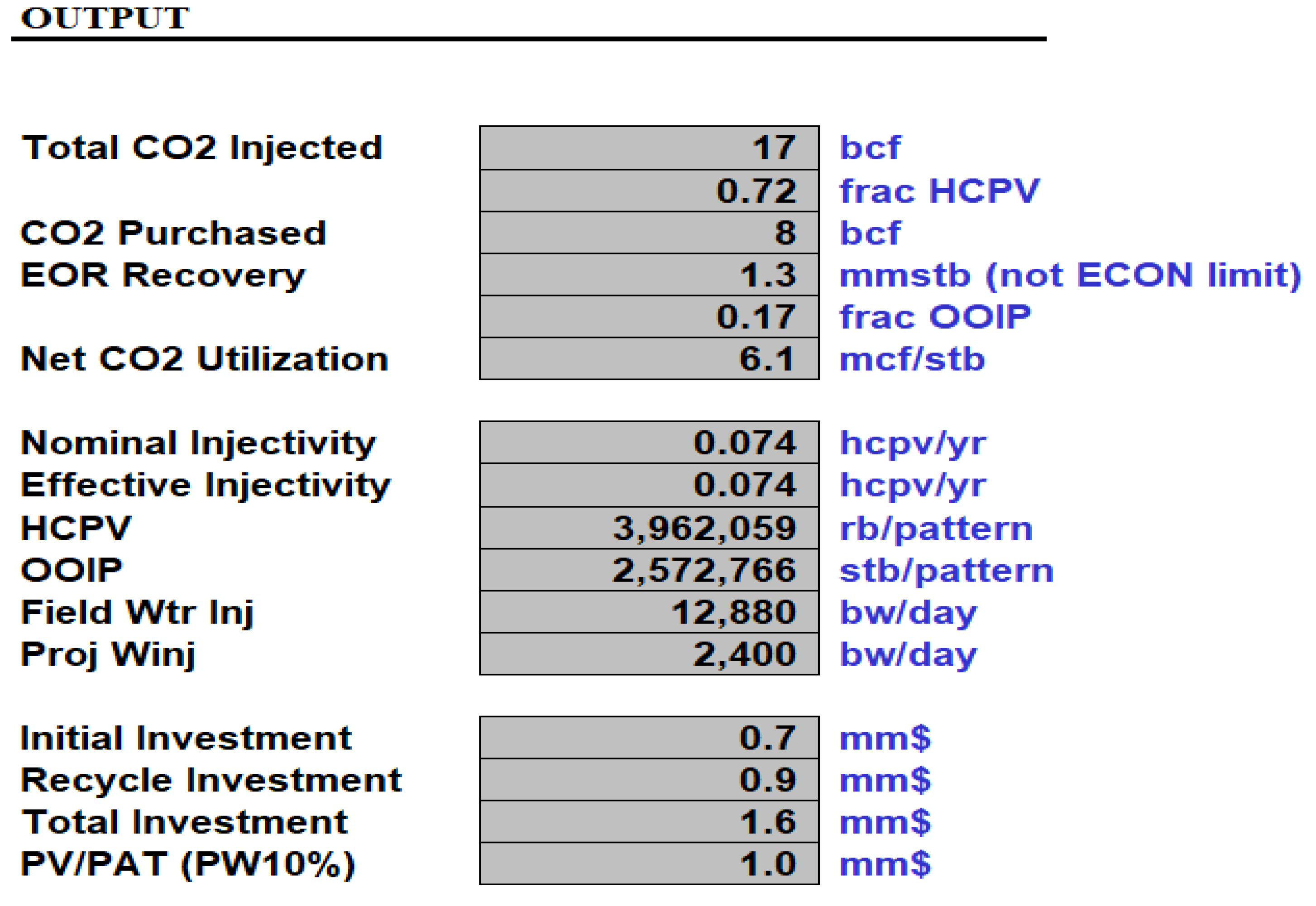
Figure 12.
Cumulative oil production against production years.
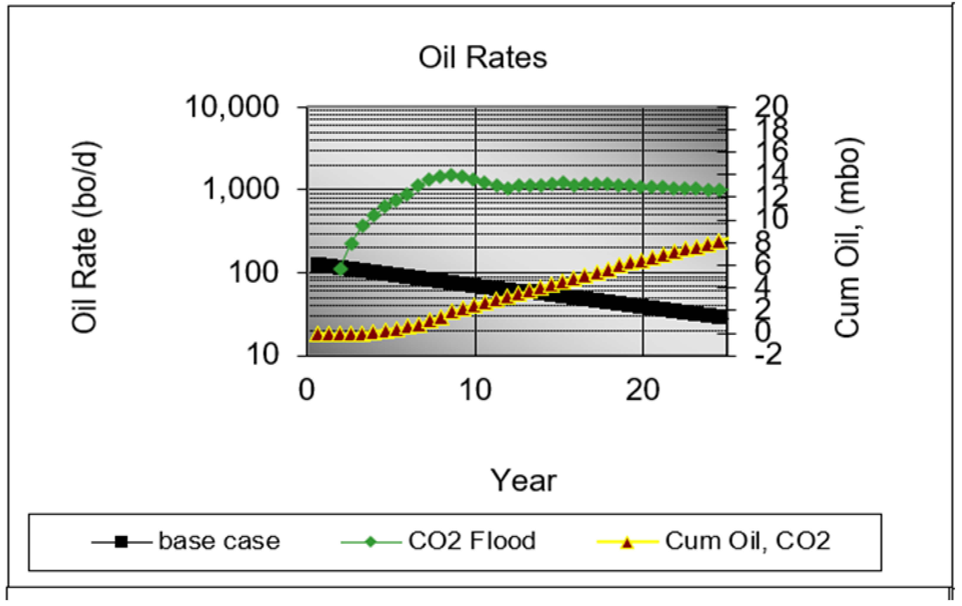
Figure 13.
History match results.
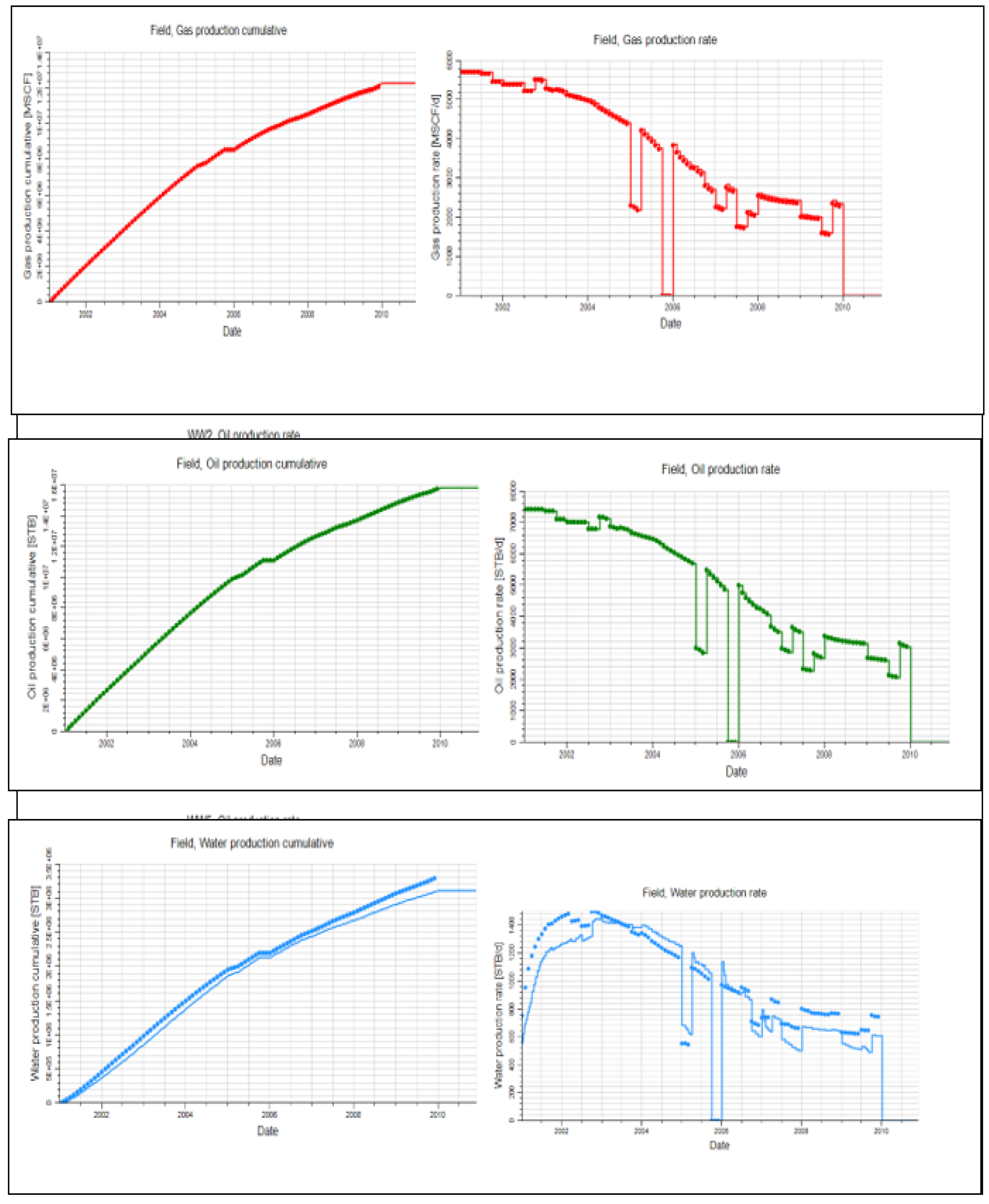
Figure 14.
History Match for the oil production rate for each well.
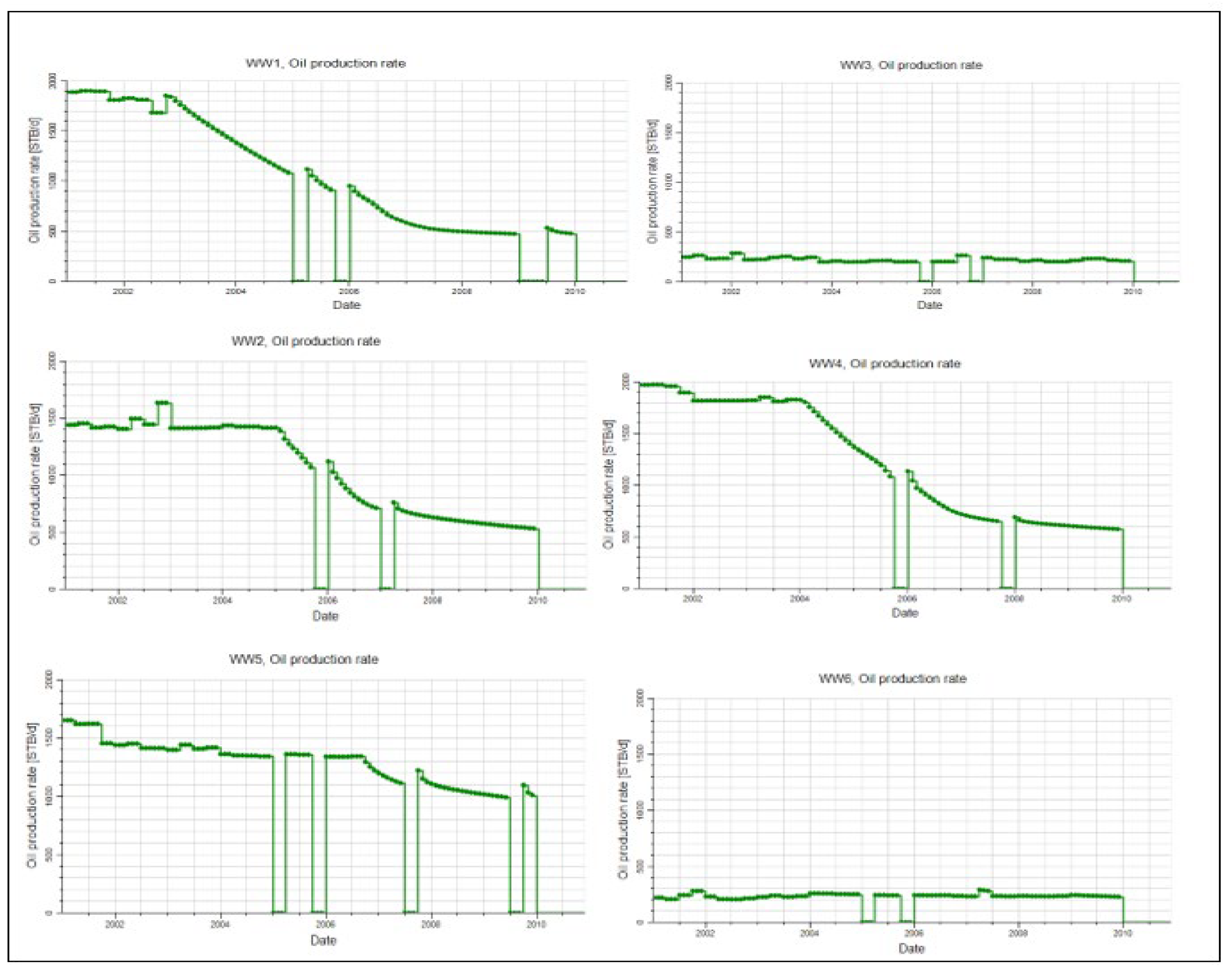
Figure 15.
History Match for the Gas production rate for each well.
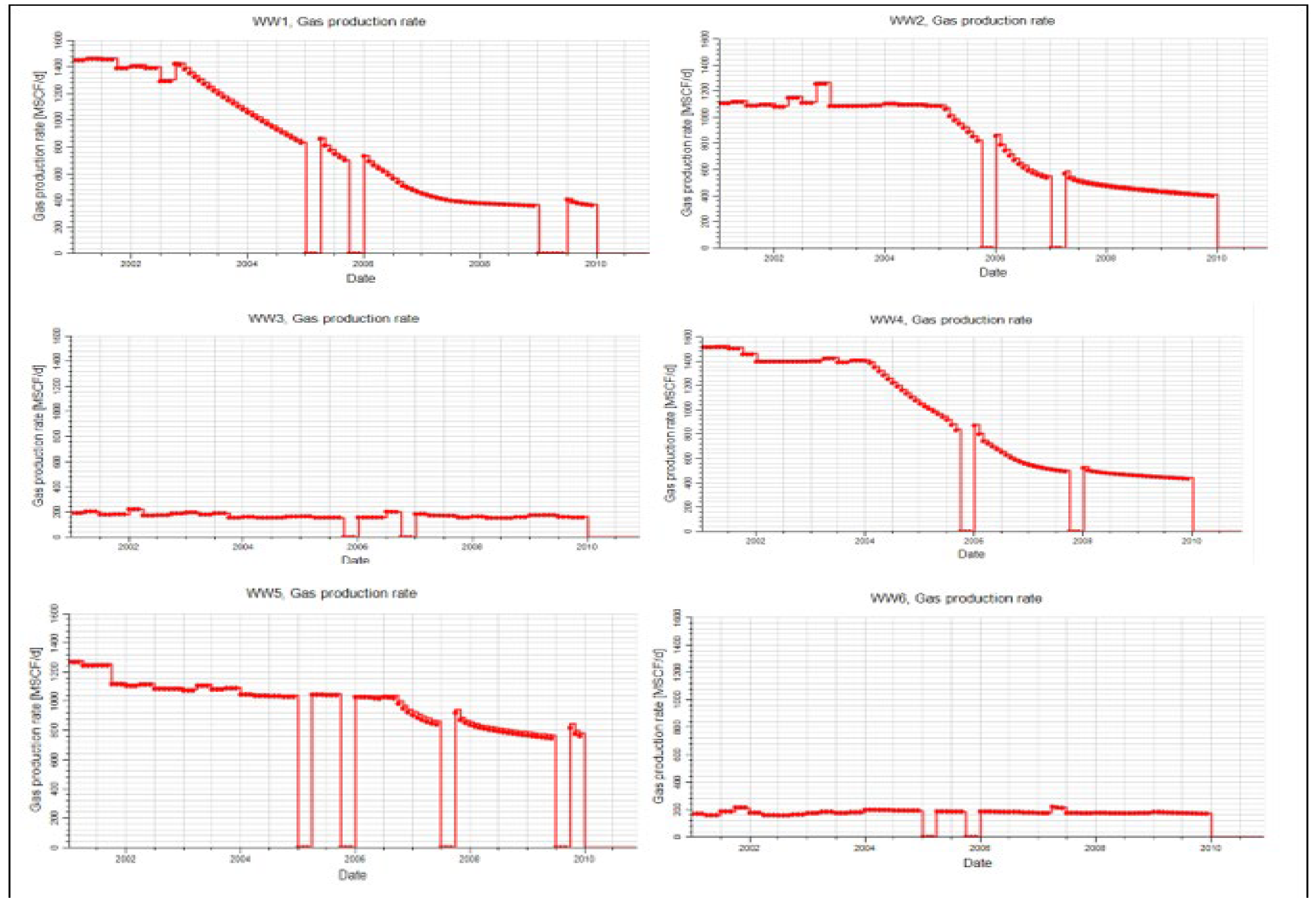
Figure 16.
History Match for the water production rate for each well.
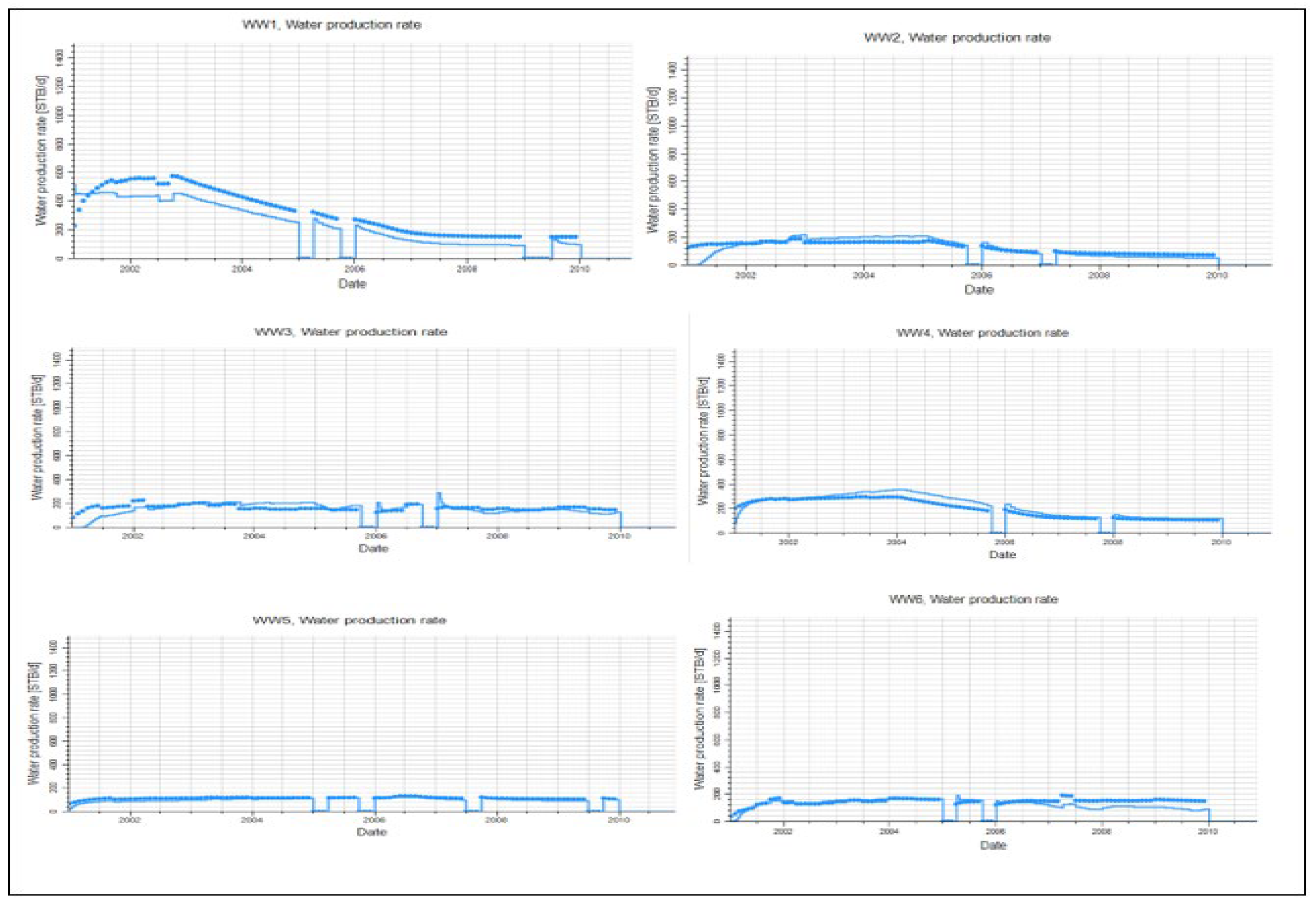
Figure 17.
History Match for the Bottom Hole pressure for each well.
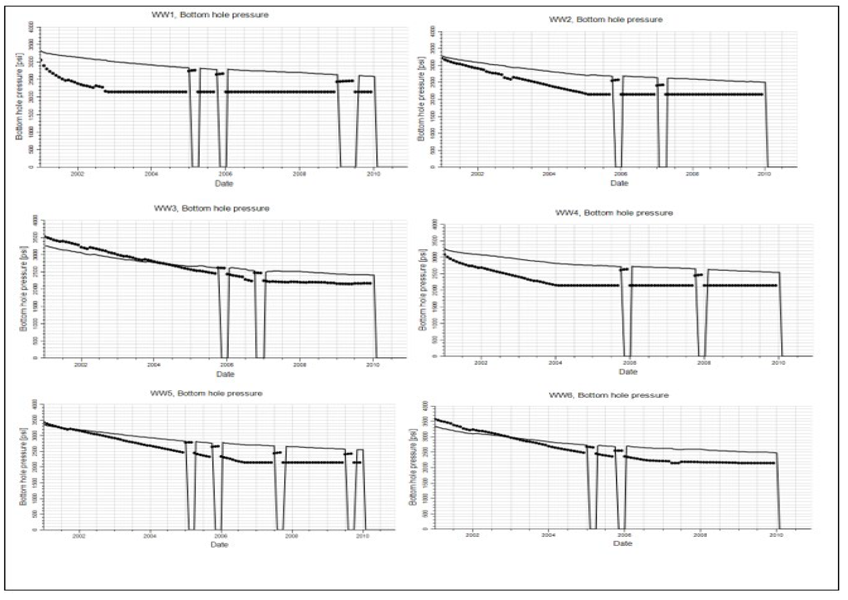
Figure 18.
Graph of pressure versus years of production showing various development scenarios.
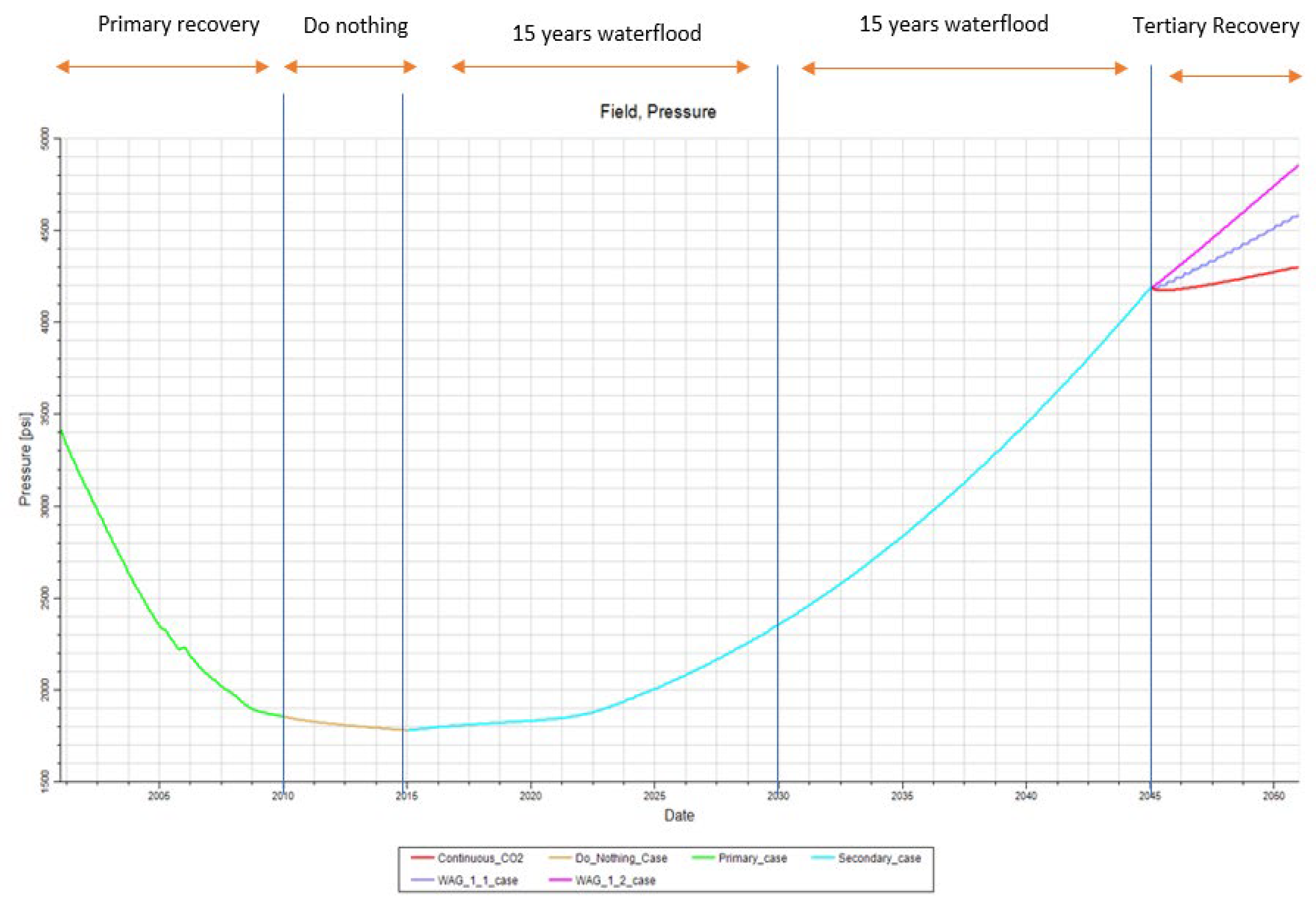
Figure 19.
pressure and cumulative oil production versus production years for primary and normal depletion.
Figure 19.
pressure and cumulative oil production versus production years for primary and normal depletion.
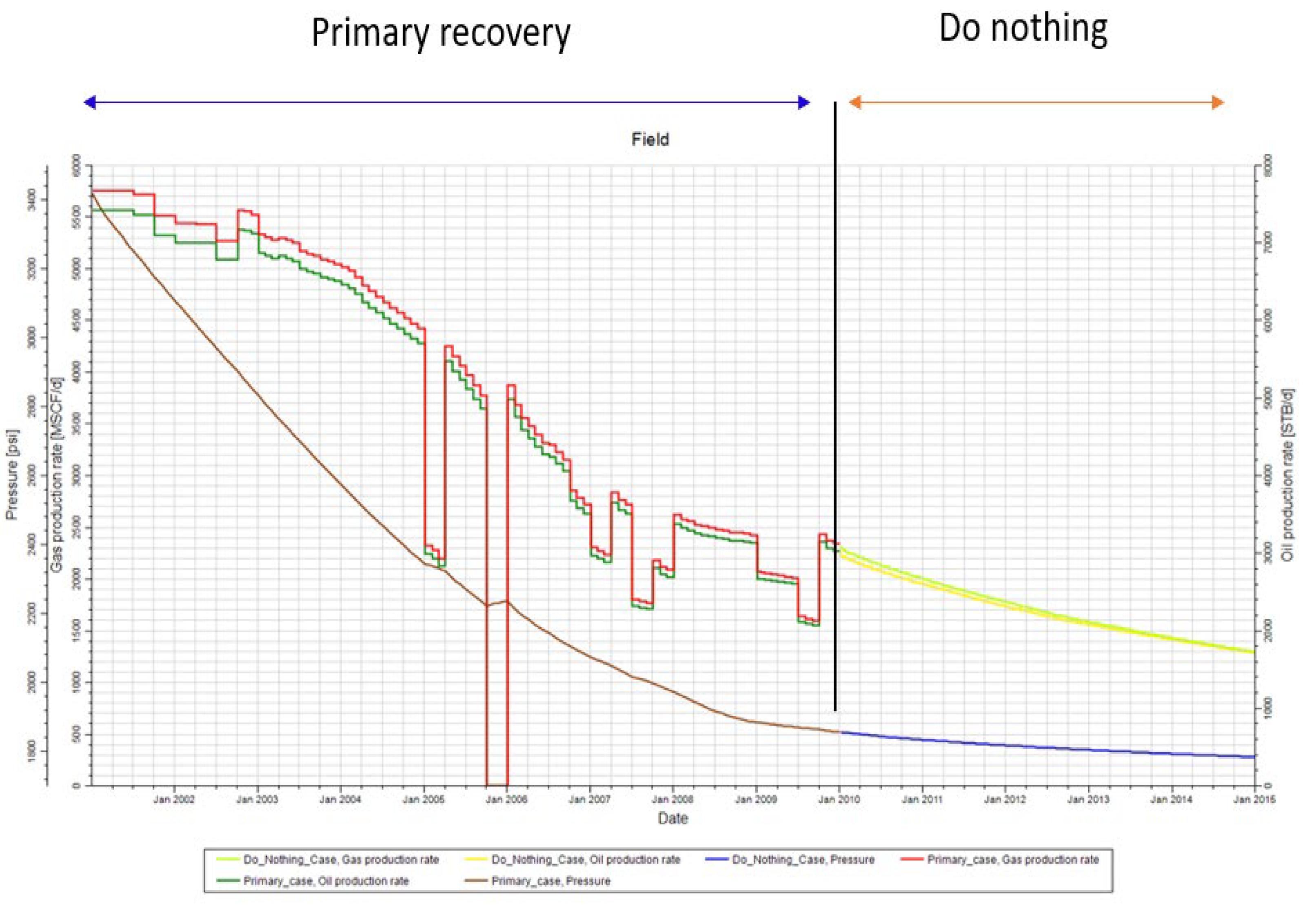
Figure 20.
Pressure and cumulative oil production versus production years for primary depletion, normal depletion and waterflooding.
Figure 20.
Pressure and cumulative oil production versus production years for primary depletion, normal depletion and waterflooding.
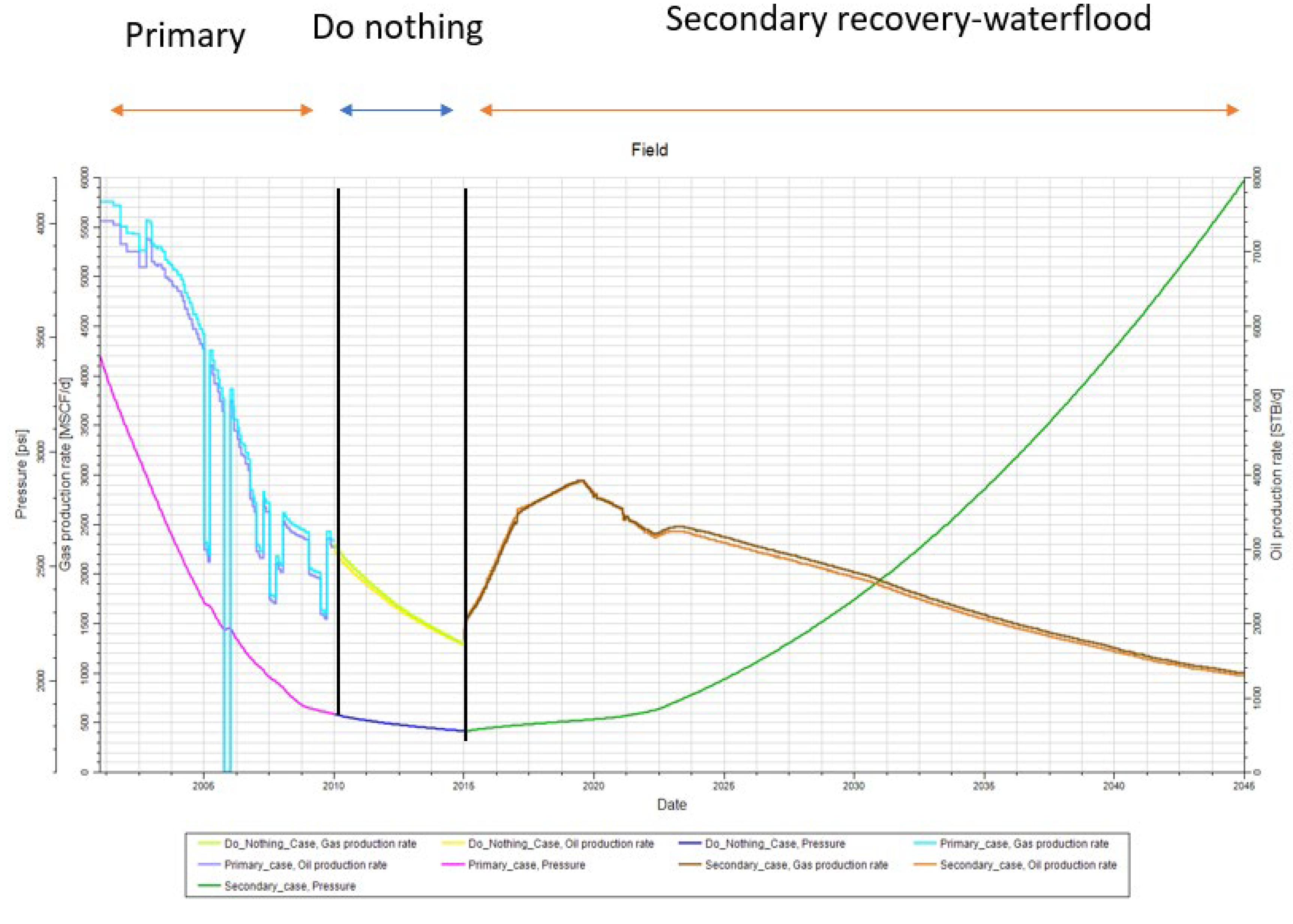
Figure 21.
Pressure and cumulative oil production versus production years for waterflooding and tertiary recovery.
Figure 21.
Pressure and cumulative oil production versus production years for waterflooding and tertiary recovery.
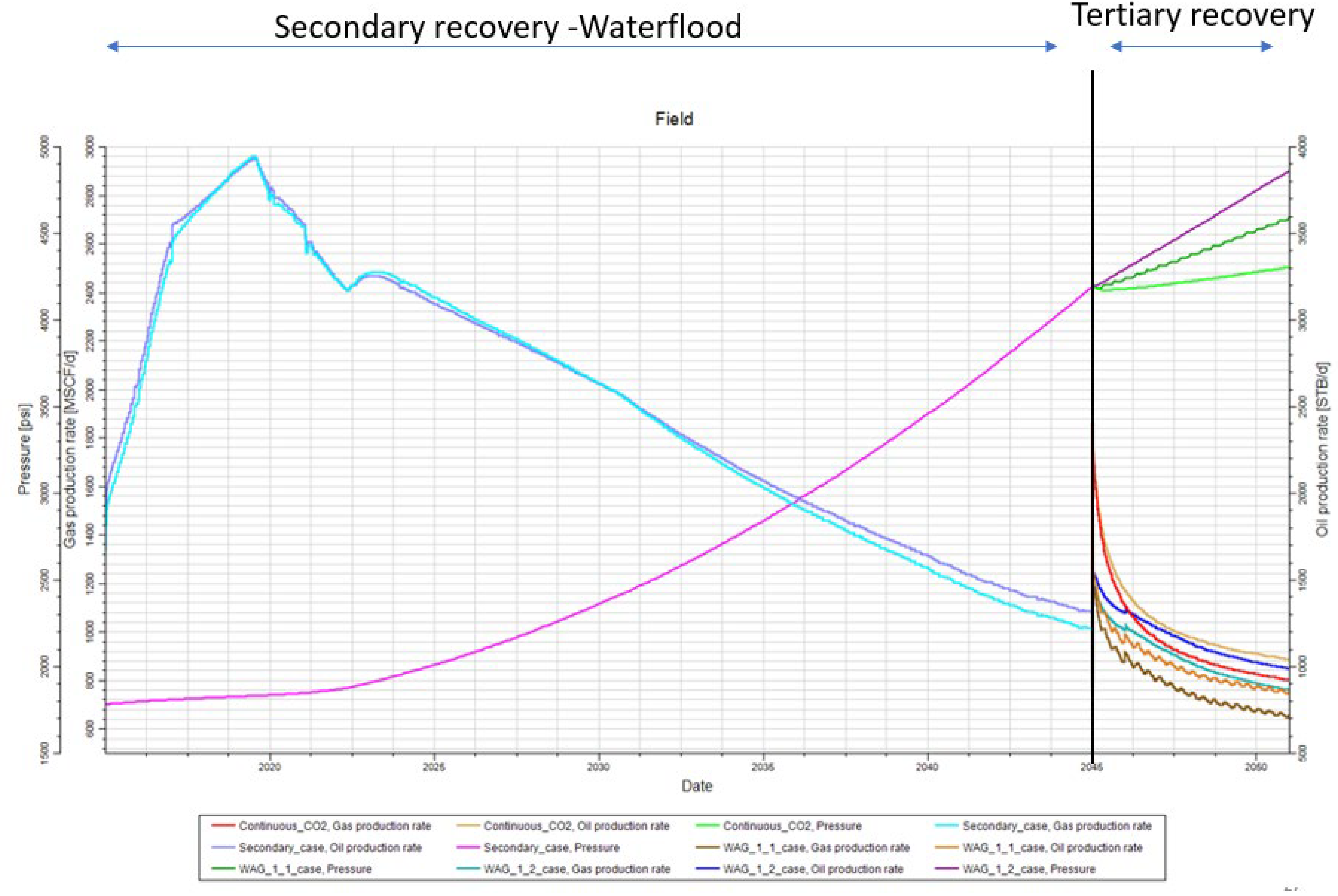
Figure 22.
cumulative oil and gas production for normal depletion.
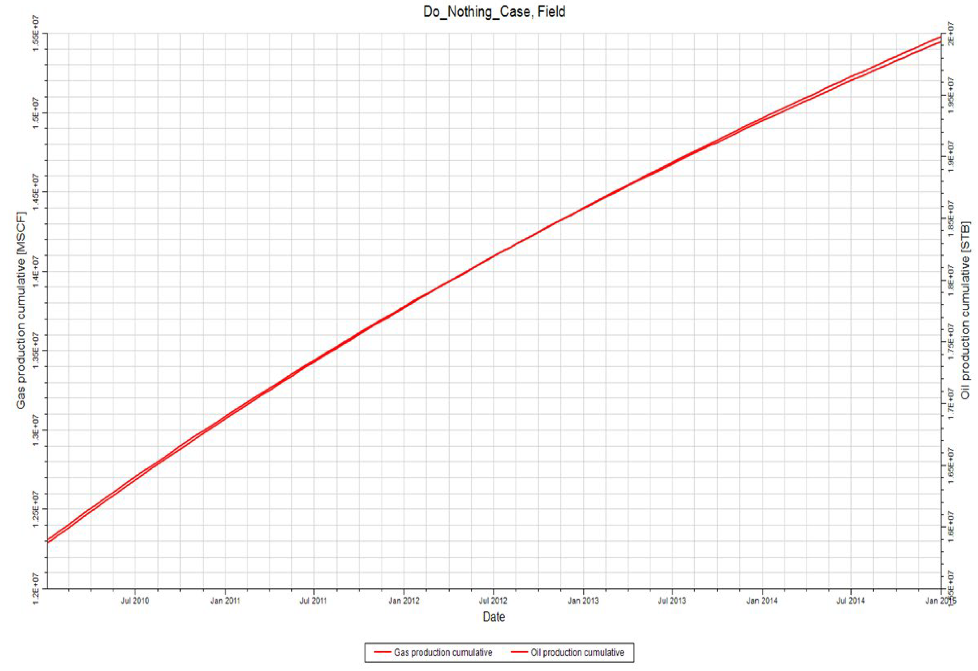
Figure 24.
Saturation maps after waterflooding.
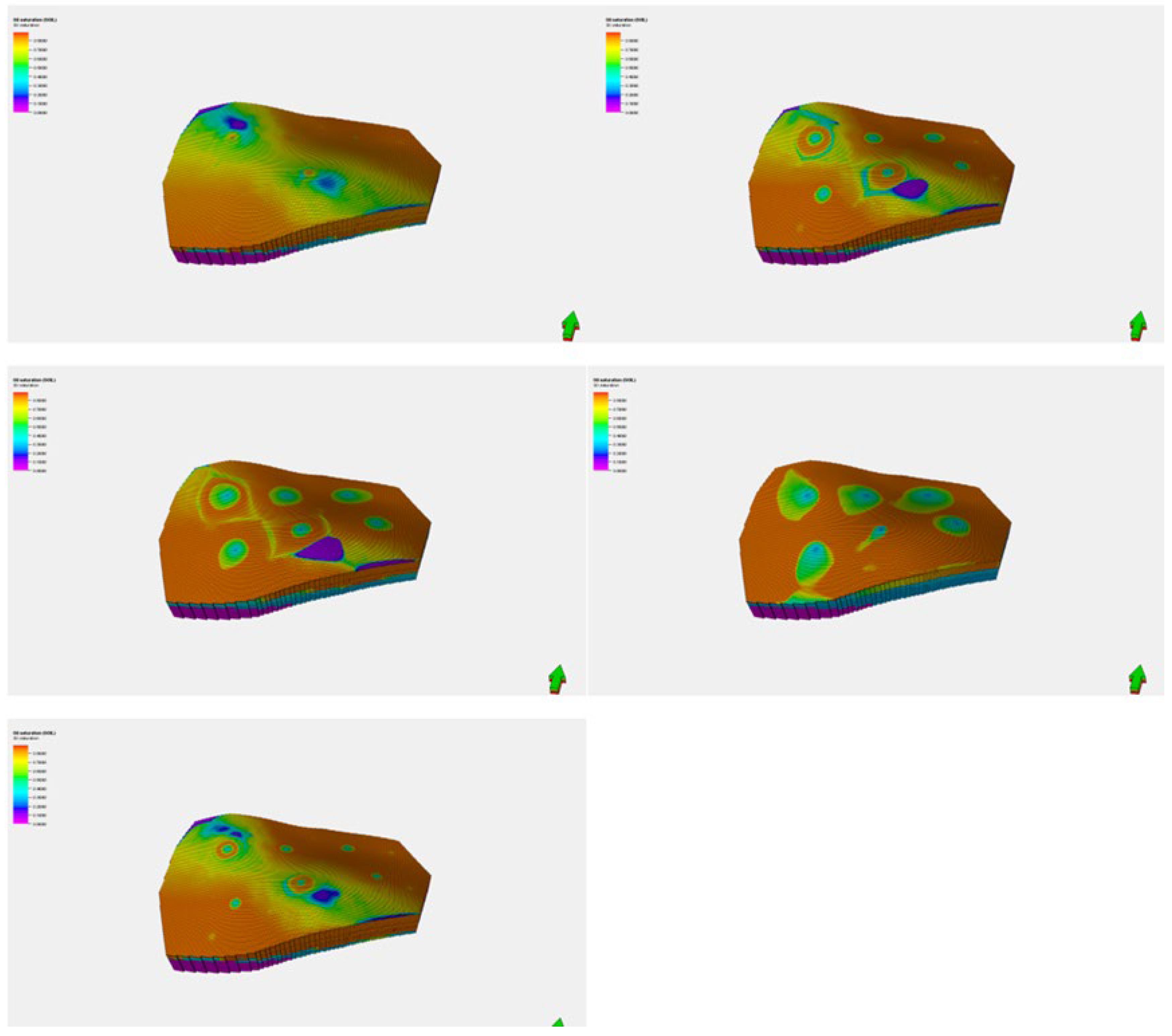
Figure 25.
cumulative Oil and Gas production for all tertiary recovery scenarios.
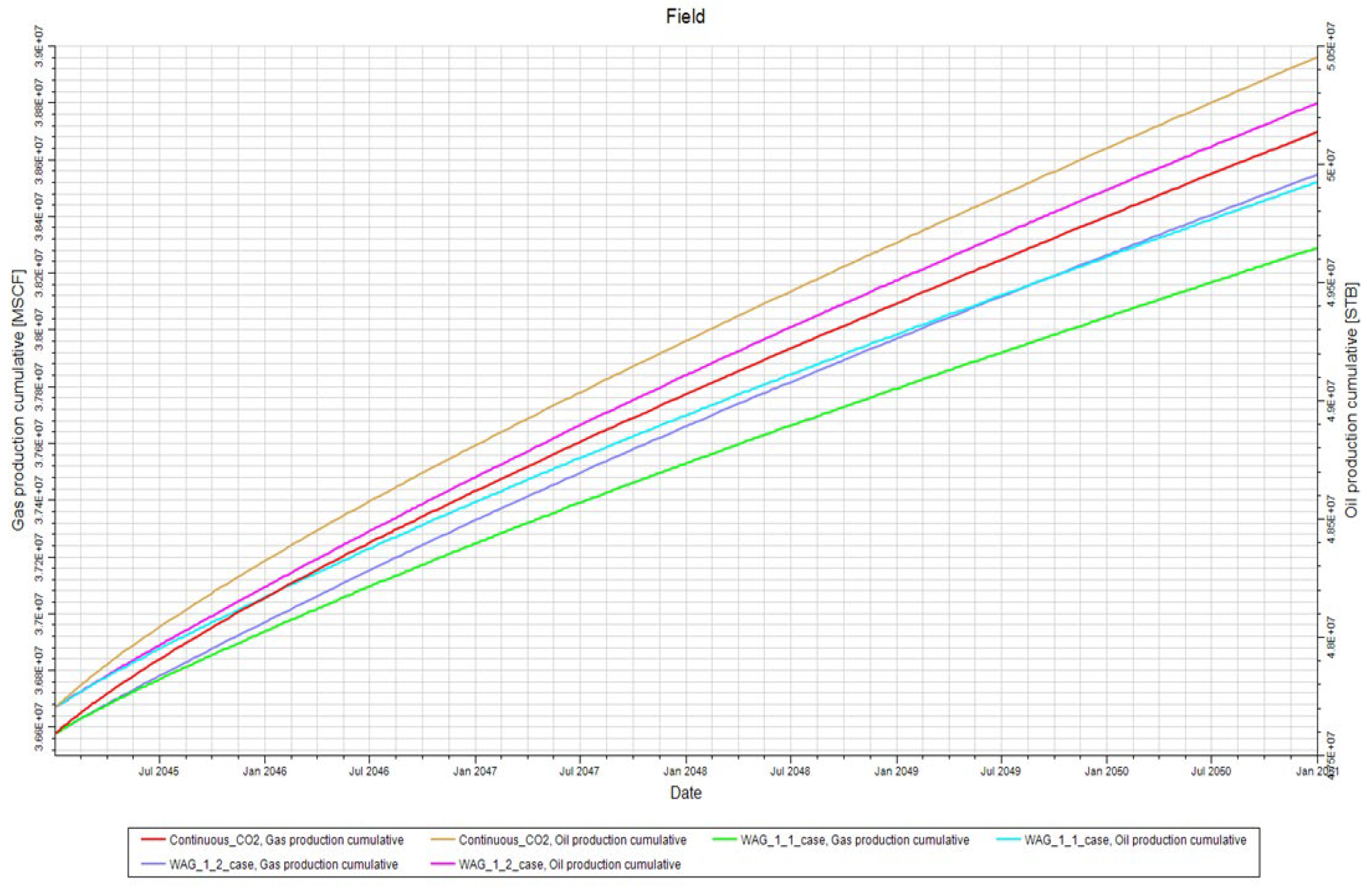
Figure 26.
streamlines after waterflooding.
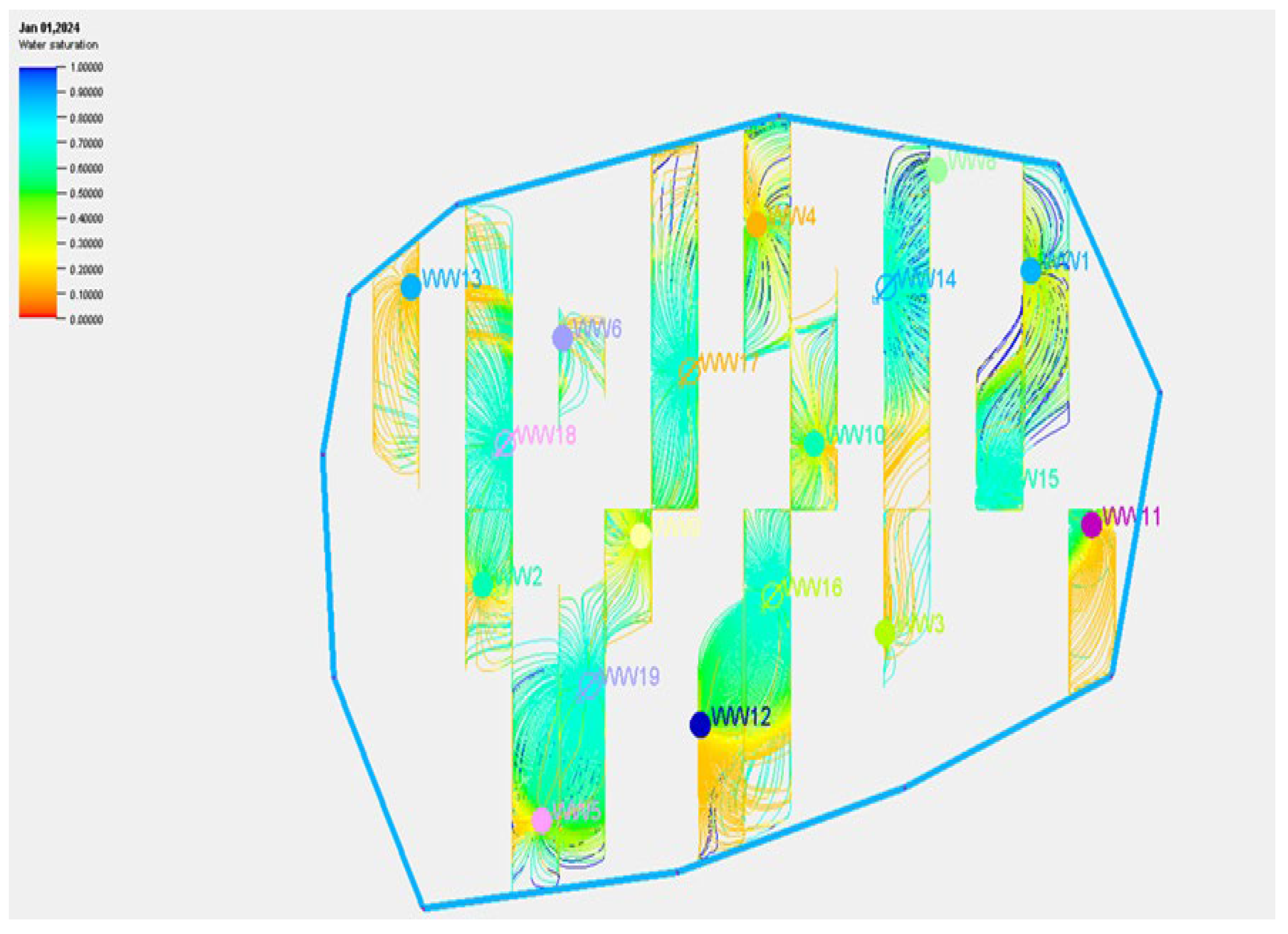
Figure 27.
Graph of pressure and oil production versus for different development scenarios.
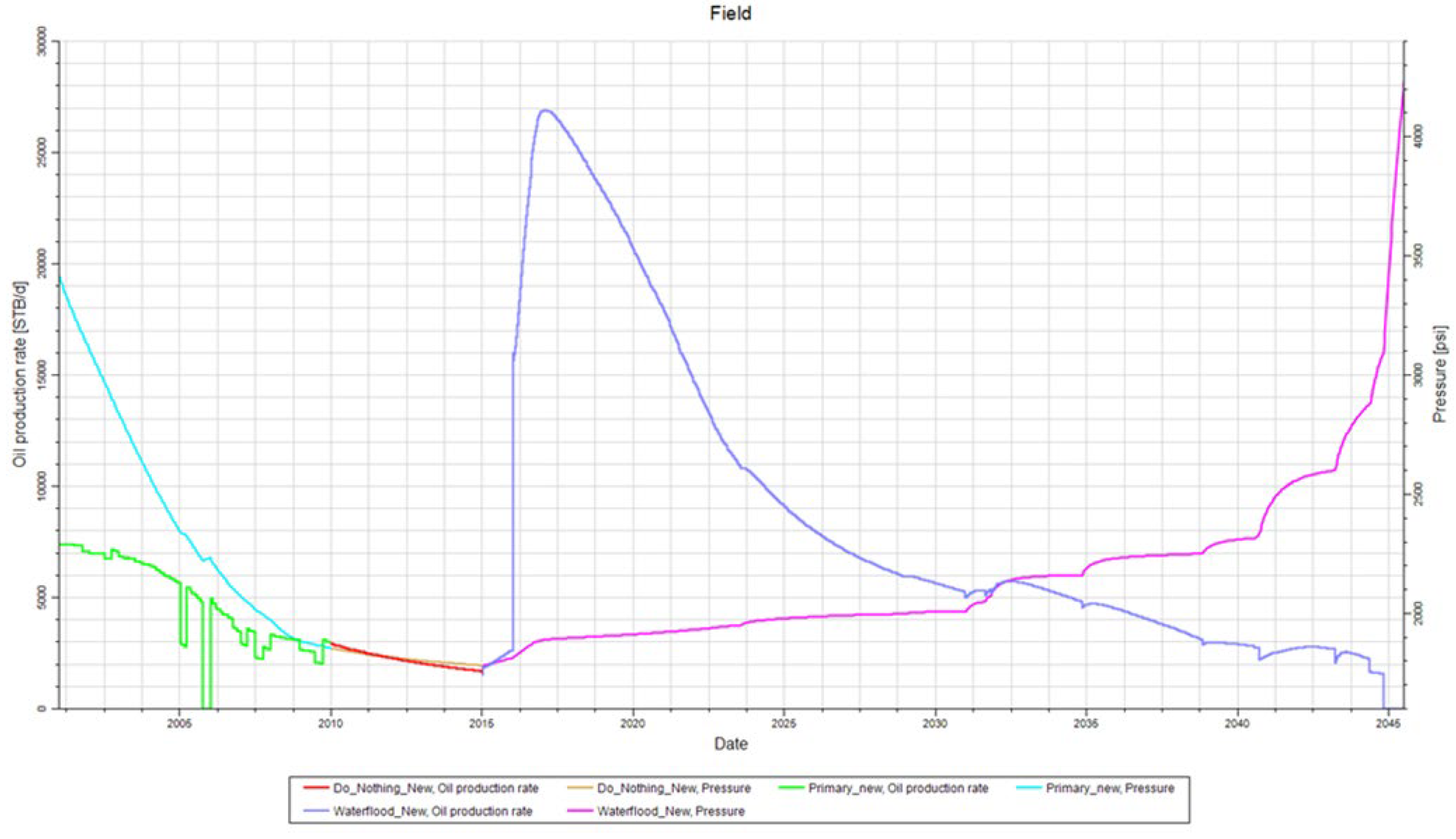
Figure 28.
cumulative oil and gas production for waterflooding.
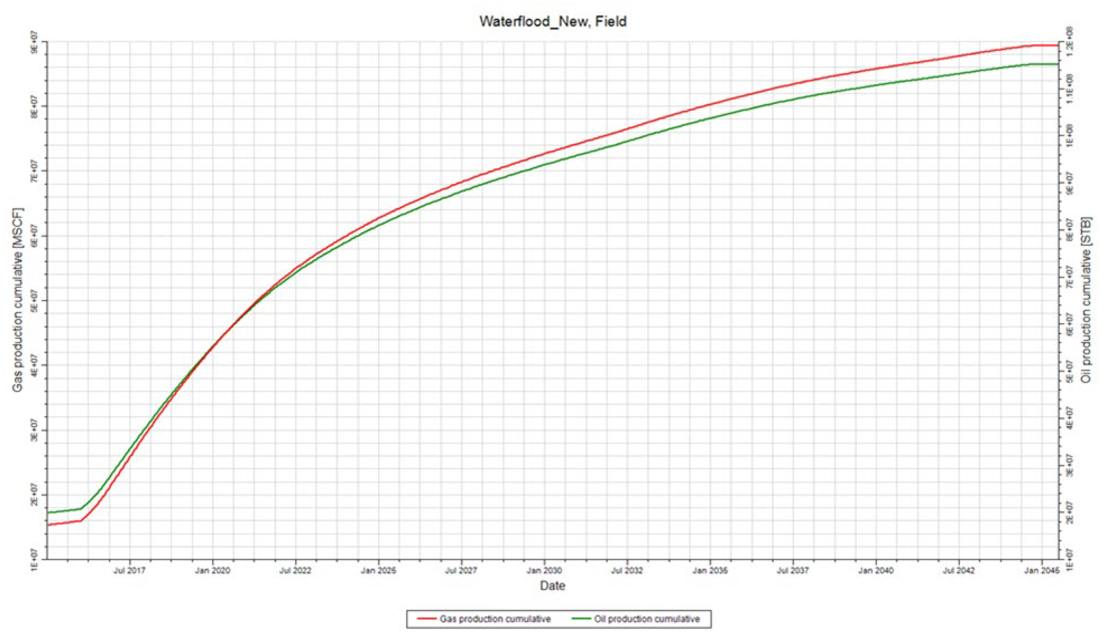
Table 1.
Summary of the simulation grid statistics.
| Model | Dimension, ft nI | nJ nK Total Cells |
| I J | ||
| Upscaled Model | 100 100 216 | 162 172 207690 |
Table 1.
Screening criteria.
| Criteria | Optimum Condition |
| Depth, ft | 2500 - 3000 |
| Reservoir Temperature, 0F | < 120 |
| Reservoir pressure, psi | > 3000 |
| Total dissolved Solids (TDS) | < 10000mg/L |
| Oil gravity | Medium to light (27- 390 API |
| Oil viscosity, cp | < 10 |
| Reservoir Type | Carbonate reservoir preferred than sandstone |
| Minimum Miscibility Pressure, psi | 1300 -2500 |
| Oil saturation | >20% |
| Net Pay Thickness, ft | 75-137 |
| Porosity | >7% |
| Permeability | >10mD |
Criteria for screening reservoirs for CO2 EOR suitability [8].
Table 5.
Various scenarios for the CO2 Prophet.
| Case 1 | Case 2 | Case 3 Case 4 Case 5 Case 6 | |
| Number of Injectors Cumulative Production (MSTB) Incremental Oil Recovery (%) Injection Mode |
3 | 3 | 3 2 2 2 |
| 9043.8 3.82 WAG |
8852 3.73 Continuous Miscible CO2 |
9043.8 63109.4 5907.4 0.1 3.82 26.63 2.49 0 Waterflood WAG Continuous Waterflood Miscible CO2 |
Disclaimer/Publisher’s Note: The statements, opinions and data contained in all publications are solely those of the individual author(s) and contributor(s) and not of MDPI and/or the editor(s). MDPI and/or the editor(s) disclaim responsibility for any injury to people or property resulting from any ideas, methods, instructions or products referred to in the content. |
© 2025 by the authors. Licensee MDPI, Basel, Switzerland. This article is an open access article distributed under the terms and conditions of the Creative Commons Attribution (CC BY) license (http://creativecommons.org/licenses/by/4.0/).
Copyright: This open access article is published under a Creative Commons CC BY 4.0 license, which permit the free download, distribution, and reuse, provided that the author and preprint are cited in any reuse.


