
Submitted:
14 May 2025
Posted:
15 May 2025
You are already at the latest version
Abstract
Managing groundwater flow in crystalline basement aquifers (CBAs) remains challenging due to their dependence on secondary permeability fields characterized by high spatial variability. This study combines pumping and tracer tests to estimate the hydraulic properties and connectivity in four bedrock wells within a CBA in southwestern Nigeria. The pumping tests caused drawdowns up to 4.13 m and 12.6 m in observation and pumping wells, with significant drawdowns only in three of four wells revealing poor connection with the fourth well. The time-drawdown plots confirm double porosity effects suggesting fracture and matrix flow and release of water from a fractured dyke. Fracture and matrix hydraulic conductivities exceeded 7.9 × 10⁻⁷ m/s and 1.0 × 10⁻¹⁰ m/s, while the aquifer yield ranged from 0.08 to 0.34%. Groundwater flow velocity and dispersivity of 5.8 × 10⁻⁴ m/s and 2.6 m were estimated from the tracer test, while a Peclet number of 3.25 suggests dominant advective flow. Calculated sustainable yield shows that each well could provide water for up to 1,600 people under controlled low pumping at 0.5 l/s with higher rates possible using larger diameter wells. These results confirm high variability in groundwater flow within CBAs, justifying the need to characterize them effectively.
Keywords:
Pumping test
; tracer test
; crystalline basement aquifer
; hydraulic conductivity
; southwestern Nigeria
1. Introduction
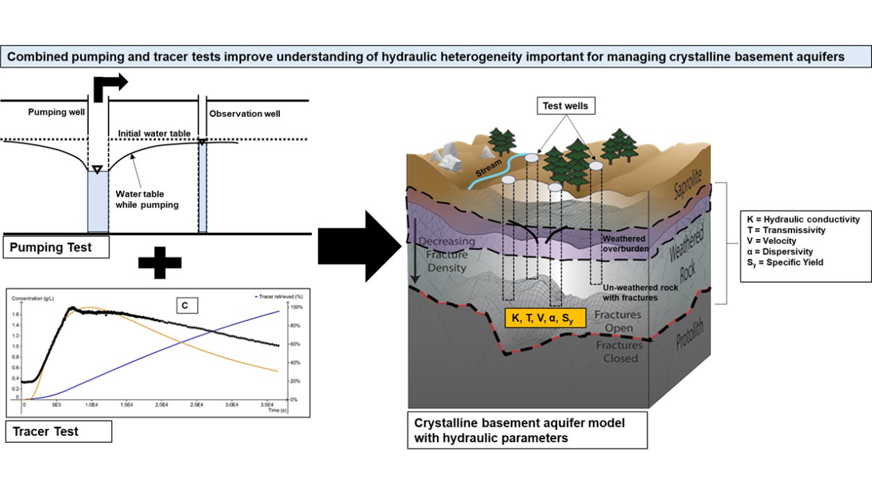
Crystalline basement aquifers (CBAs) are significant sources of drinking water in most parts of sub-Saharan Africa, including Southwestern Nigeria [1] despite being characterized by low hydraulic conductivity and specific yield [2,3]. Sustainable management of these critical water resources requires understanding the aquifer yield and the distribution of their hydraulic properties and connectivity [4,5]. The hydraulic properties, including transmissivity, hydraulic conductivity, storativity, flow velocity, and dispersivity, are essential for informing groundwater models used to predict flow and transport within these aquifers [6,7]. Limited studies have, however, investigated the hydraulic properties distribution and connectivity within CBAs in southwestern Nigeria, which are inherently heterogeneous [8]. This study presents a field assessment of hydraulic properties variation, connectivity and sustainable yield of a CBA at the Ibadan Hydrogeophysics Research Site in southwestern Nigeria using multiple pumping and tracer tests.
CBAs are formed by intense weathering and fracturing of impermeable igneous and metamorphic rocks such as granite and gneiss, creating regolith of varying thickness, which overlies crystalline rocks with discontinuities such as fractures, joints, and faults [9,10,11]. Generally, the geometry of CBAs consists of a topsoil layer, a weathered overburden termed saprolite, a weathered and fractured crystalline rock termed saprock, and a fresh crystalline rock serving as an aquitard [2]. CBAs exhibit complex groundwater flow characteristics due to their low primary porosity and dependence on secondary porosity created by fractures, joints, faults, and weathering [12].
The intensity and connectivity of fractures determine the hydraulic properties such as hydraulic conductivity controlling flow and transport within these aquifers [13,14]. In intensely fractured zones, groundwater flow is enhanced due to increased hydraulic conductivity, whereas in areas with sparse or poorly connected fractures, groundwater flow is significantly restricted [15,16]. Also, groundwater storage and transmission within CBAs are strongly affected by the degree of weathering within the crystalline basement rocks [17]. The weathered zone or regolith consisting of weathered crystalline rock and clay-rich material stores considerable amounts of water [11,18]. However, the high clay content reduces its hydraulic conductivity, restricting groundwater movement [2]. The transition zone between the weathered layer and the fractured bedrock allows water storage which recharges the fracture basement [19,20,21]. The complex geology, weathering, and fracture distribution within CBAs make their flow and transport properties vary over several orders of magnitude [14].
The high variability in hydraulic conductivity and other flow and transport parameters poses significant challenges in groundwater assessment and management within crystalline basements [2,22]. Unlike sedimentary aquifers, where flow properties are relatively less variable, CBAs exhibit localized high-permeability pathways interspersed within low-permeability rocks [14,23]. This heterogeneity complicates the prediction of groundwater flow and contaminant transport, requiring advanced hydrogeological investigations and modeling approaches. Quantifying these variations necessitates the use of geophysical surveys [24,25], hydraulic testing, and numerical modeling techniques, all of which are constrained by inherent uncertainty [4,6,26,27].
Hydraulic testing, including pumping and tracer tests, has been widely used to estimate the variation in aquifer flow and transport properties [28,29,30,31]. Pumping tests are used to estimate aquifer transmissivity, hydraulic conductivity, and storativity by analyzing the drawdown response to pumping in wells over time [32,33,34]. These tests typically involve withdrawing water at a constant or stepwise varying rate from a well while monitoring the resulting water level changes in both the pumping and observation wells [31]. The interpretation of pumping test data relies on analytical and numerical models that assume aquifer homogeneity, isotropy, and confined or unconfined flow regimes [35,36,37]. For fractured crystalline basement aquifers, drawdown curves often deviate from the idealized Theis-type response, reflecting the dual-porosity nature of these systems, where groundwater flow occurs both within the fracture network and the surrounding rock matrix [38,39]. The presence of fractures can lead to early rapid drawdown followed by a delayed response due to matrix diffusion and storage effects [40,41]. Additionally, time-drawdown analysis can reveal whether the aquifer behaves as a single or double porosity system, with fracture-dominated flow exhibiting a characteristic non-linear decline in drawdown over time [42,43].
Besides the classical constant-rate pumping tests, step-drawdown tests, in which the pumping rate is increased in discrete steps, are also used to assess the well efficiency and to identify turbulent flow effects near the wellbore [44,45]. The interpretation of step-drawdown data allows for distinguishing between laminar and turbulent flow components, which is crucial for understanding the impact of well losses on measured hydraulic properties [46]. After a pumping test is completed, the recovery of the well can also be monitored with time by recording the rate at which the water level recovers to its original static level. Recovery data provide an alternative means of estimating transmissivity and storativity while minimizing potential errors associated with well losses and boundary effects [47]. The interpretation of recovery tests is typically based on the Theis recovery method, which assumes that drawdown and recovery curves mirror each other when plotted semi-logarithmically [34,47]. However, in fractured aquifers, recovery trends may deviate from conventional porous media behavior due to delayed water release from fractures and the surrounding matrix [39,40,48,49]. Recovery tests are particularly useful in cases where drawdown data are ambiguous or affected by external influences such as recharge or interference from nearby wells [49].
Tracer tests also provide complementary information on groundwater flow velocity, dispersivity, and connectivity between wells. These tests involve the injection of a tracer (e.g., sodium chloride, or fluorescein) into an injection well and monitoring its breakthrough at downstream observation or extraction wells [1,50]. The time taken for the tracer to appear, its peak concentration, and its tailing behavior provide valuable insights into the dominant transport mechanisms within the aquifer. The interpretation of tracer test results depends on the nature of groundwater flow within the aquifer. In porous media, solute transport is typically governed by advection and hydrodynamic dispersion [51]. However, in fractured crystalline aquifers, solute movement is often dominated by advection through high-permeability fractures and diffusion into the surrounding low-permeability matrix [52,53]. The Peclet number (Pe), which describes the relative importance of advection versus dispersion, helps characterize the transport regime within the aquifer. A high Pe value suggests that advection dominates, whereas a low Pe value indicates significant diffusive mixing [54]. Tracer breakthrough curves (BTCs) can exhibit pronounced tailing due to matrix diffusion, where solutes temporarily migrate into low-permeability zones before re-entering the main flow path [55,56,57]. The shape of BTCs also reveals the degree of fracture connectivity; well-connected fractures produce sharp breakthrough peaks, while poorly connected systems exhibit delayed and dispersed arrival times [58].
Despite the established importance of pumping and tracer tests in groundwater characterization, few studies have applied both techniques to systematically evaluate the variation in hydraulic properties and connectivity of crystalline basement aquifers in southwestern Nigeria. This study aims to estimate key hydraulic parameters (e.g., hydraulic conductivity and storativity) using constant-rate and step-drawdown pumping tests. Fracture connectivity and groundwater flow velocity are assessed using pumping and a salt tracer test. The transport behavior of solutes within the crystalline basement aquifer is evaluated using the tracer breakthrough curves. The hydraulic test results are then compared with existing conceptual models of fractured basement aquifer flow to improve the understanding of groundwater behavior in similar geological settings. By integrating pumping and tracer test data, this study provides an assessment of groundwater flow and transport processes in a crystalline basement aquifer, which is essential for sustainable water resource management. Results of this study will inform hydrogeological modeling and support decision-making for groundwater development in fractured rock environments.
2. Study Site
This study was conducted at the Ibadan Hydrogeophysics Research Site (IHRS) located within the University of Ibadan campus in Oyo State, Nigeria. The site serves as a field research laboratory for advancing the understanding of hydrological processes within crystalline basement aquifers in parts of the country with similar architecture and as a guide for studies in regions where the crystalline basement aquifer has a significantly different architecture, e.g., a thicker weathered zone and a deeper active fractured zone. The study area is part of Southwestern Nigeria’s Precambrian basement complex which is dominated by augen gneiss, granite gneiss, banded gneiss, quartzites, and migmatites with the intrusion of pegmatite and dolerite dyke, covered by weathered superficial sediments [59,60,61,62]. Major faults trending northwest and southeast have been mapped in the area [63], with multiple fractures oriented northeast and southwest serving as major sources of groundwater supply [64]. The study area covers approximately 15,000 m2 in size, within coordinates 7˚ 28ʹ 24ʺ to 7˚ 28ʹ 26ʺ Easting and 3˚ 53ʹ 52ʺ to 3˚ 53ʹ 54ʺ Northing and elevation ranging from 205 m to 212 m above mean sea level (Figure 1). The site is bounded to the north by a perennial stream that flows NW-SE, to the east by a road, and to the south and west by a cultivated farmland [4,65].
The site was established in 2019 with four bedrock groundwater wells drilled down to 30 m. Lithology logs, prior geological observations, and electrical resistivity tomography profiles of the site indicate that the hydrogeological units consist of an overburden made up of clayey sand and clay, as shown in the lithological section of the wells in Figure 2. The clay-rich top layer is underlain by the weathered basement rocks, the fractured rocks, and lastly, the fresh basement rocks [65,66].
3. Materials and Methods
3.1. Constant-Rate Pumping Test
Constant rate pumping tests have been conducted in several aquifer characterization projects that give a step-by-step guide to conducting such tests [67,68,69,70]. For this study, we conducted constant-rate pumping tests at all four wells at the site by first pumping at well A (Figure 1) at a constant rate of 0.9 l/s while simultaneously monitoring groundwater level changes (drawdown) in the pumping well (well A) and the other wells which served as observation wells (wells B, C and D). We then repeated the test by pumping wells B, C, and D, respectively, while measuring drawdown in the pumping and observation wells in each case. A submersible pump installed at a depth of ~25 m was used for pumping, while the observation and pumping wells were equipped with automated CTD Diver data loggers (VanEssen Instruments, Tucker, GA, USA) to take temperature, electrical conductivity, and water level measurements every 30 seconds. A flow meter was installed to monitor the extraction rate every 10 minutes, and the mean flow rate of 0.9 l/s was used for data processing. Manual water level measurement was also performed using a battery-powered water level meter, beginning with a thirty-second interval for the first hour and progressing to a one-minute interval for the next hour, two minutes for the next hour, and finally, every five minutes until the exercise was completed. Two cycles of pumping tests were conducted for all four wells, with the first lasting for 9 hours and the second lasting for 12 hours, giving a total of 8 constant rate pumping tests. During each test, the extracted water was discharged far away from the research site via a network of pipes to avoid reabsorption into the pumped aquifer. To ensure that the aquifer had fully recovered before carrying out successive tests, we allowed a break of at least 72 hours before successive pumping exercise. Two days before conducting the pumping test, all four wells were also developed to ensure a good connection to the aquifer.
Time series of hydraulic head measurements during each pumping test were pressure-compensated to account for the effects of changing atmospheric pressure during the test using barometric pressure measured simultaneously for the same period using a Van Essen CTD Diver baro-logger. Changes in the hydraulic head with respect to the starting hydraulic head were used to estimate drawdown. Linear, semi-log, and log-log plots of drawdown with time were used to assess the aquifer’s water level response to pumping. Analyzing the pumping test drawdown versus time data required fitting an appropriate analytical solution to the data to estimate the aquifer hydraulic properties. To choose an appropriate model for the data, we first compared the measured drawdown data to established hydrogeologic signatures represented in the site [33,70]. We also plotted a logarithmic derivative of drawdown as a function of time and compared that with standard derivative plots (van Tonder et al., 2001) to assess the hydrogeological and boundary conditions at the site. Drawdowns in the pumping and monitoring wells were matched with type curves of analytical models while derivate analysis techniques developed by Bourdet et al. [71] were used to identify characteristic patterns representing different flow regimes in the aquifer which help to identify the aquifer flow regime needed for constructing a hydrodynamic conceptual model. Analysis of the derivative and diagnostic plots were used to identify boundary conditions and flow regimes such as the well-bore storage effect, fracture dewatering effect, double-porosity, and radial flow diagnosis [70].
We fitted semi-log and log-log plots of drawdown versus time with an analytical solution by Baker [40] for a generalized radial flow (GRF) in fractured aquifer [40] implemented in the AQTESOLV software (Hydrosolve, Inc, Virginia, USA). The model’s best fit was used to estimate the fracture and matrix hydraulic conductivities, the fracture and matrix specific storage and the effective dimension number (n-dimension) of the fractured aquifer [70]. With the aquifer conceptualized as an unconfined aquifer, we expect the specific yield to be much greater than the specific storage. Hence, we calculated the specific yield following Remson and Lang’s [72] approach by comparing the volume of dewatered material in the cone of depression with the total volume of water discharged during the pumping exercise. The specific yield is given as:
where
T is transmissivity (product of hydraulic conductivity, K, and the aquifer thickness, b), r is the horizontal distance from the axis of the pumped well to a point on the cone of depression, s is the drawdown at distance r, Q is discharge and V is volume of dewatered material.
Based on the groundwater discharge during the pumping tests in each of the wells, we computed the sustainable yield using the flow characteristics method (FC-Method) presented by van Tonder et al [70]. The sustainable yield describes the discharge rate that will not cause the water level in the borehole to drop below a prescribed limit (usually the position of a major water strike), to avoid the borehole drying up [73,74].
3.2. Step Drawdown Tests
During this study, we also conducted two step-drawdown tests in wells C and D (Figure 1) to assess the well performance, including well loss, well efficiency, well bore skin factor, and effective well radius in the fractured aquifer system. Pumping at each well started with an extraction rate of 0.35 L/s for the first three hours, which increased to 0.65 L/s between 3 to 6 hours of extraction, and lastly to 0.88 L/s for the final six hours following recommendations by Kruseman and De Ridder [33]. A gauge valve was installed at the extraction well to control the flow rate, which was monitored using a flow meter. Data loggers in the pumping and monitoring wells with similar settings as used for the constant rate pumping tests were used for the step drawdown tests.
Similar compensation and processing steps were followed as that of the constant-rate pumping data processing. The data was further analyzed using the Hantush and Jacob [75] model implemented in the AQTESOLV software. Hantush and Jacob [75] constructed a rigorous mathematical model of the transient flow of water at different constant pumping rates in a well in an infinitely large homogeneous, isotropic, and leaky-constrained aquifer.
3.3. Recovery Tests
The aquifer's recovery (i.e., the increase in water level) after pumping has stopped was monitored for all the pumping test scenarios. Since the recovery data is less noisy than pumping data due to fewer external perturbations during data acquisition, it helps to better understand aquifer connectivity and transport rate, both of which are critical in understanding aquifer sustainability [68]. Following each pumping test, the aquifer's recovery was monitored for 2 to 14 days using the data loggers used for the pumping tests. Our goal was to achieve full recovery and ensure that the aquifer returned to its stable ambient condition before successive pumping tests. The hydraulic head recovery (termed residual drawdown) versus time data were plotted to show the water return relationship in all the wells. The recovery data was corrected for barometric influence and analyzed using the Agawal method, which is a modified Theis method implemented in the AQTESOLV software [76].
3.4. Tracer Test
We conducted a convergent forced gradient flow field tracer test with continuous water extraction at well A and tracer injection at well C (Figure 1) to assess the connection between the wells and determine the groundwater flow velocity, average porosity and dispersivity. The tracer solution was prepared in an inflatable pool by mixing 40 kg of table salt (NaCl) with 3,240 litres (3.24 m3) of water with an ambient electrical conductivity of 0.52 mS/cm. After mixing, the electrical conductivity of the tracer was 28 mS/cm. Prior to the tracer injection, we extracted water from well A (extraction well) at 0.9 l/s for two hours using a submersible pump to create a quasi-steady state flow condition. The tracer was then injected into well C at a rate of 0.5 L/s over two hours while continuing pumping at the extraction well to maintain an undisturbed flow field. A 0.5 inches diameter hose was used to lower the tracer at a depth of 15 m while a submersible pump was installed in the injection well at a depth of 25 m to pump water from the lower section of the injection well and was re-injected at the top (at 5 m) to ensure continuous mixing of the saline tracer in the injected well. After the tracer injection, we continued pumping water at the same rate from the extraction well for 8 hours, 25 minutes to maintain the flow field. The total duration of the tracer test (pre-injection, injection, and post-injection phases) was 12 hours and 25 minutes.
Automated loggers were installed in all four wells at the site to monitor water level, temperature, and electrical conductivity. To monitor the tracer breakthrough, we used a Hannahn HI9811-51 conductivity meter (Hanna® Instrument Woonsocket, RI, USA) to measure continuously the electrical conductivity of water discharged from the extraction well. The time-series tracer data were analyzed to obtain the tracer’s first and peak arrival times, estimate the recovered tracer mass, and assess the shape of the tracer breakthrough curve. The tracer test data were further analyzed with the BRGM (French Geological Survey)’s TRAC software using the radial convergent transport model to estimate the flow velocity and dispersivity [77]. An analytical solution of the classical advection-dispersion equation was fitted to the normalized concentration – time curve to estimate the tracer transport properties.
4. Results
4.1. Constant Rate Pumping Tests
Pumping from the CBA at the study site at 0.9 l/s for 9 and 12 hours resulted in drawdowns ranging from 4.94 to 12.47 m and 5.43 to 12.58 m (Table 1) in the pumping wells with the minimum drawdown observed while pumping from well A and the maximum observed while pumping from well B. Corresponding drawdowns in the observation wells ranged from 1.63 to 3.63 m during the 9 hours pumping test and 2.03 to 4.13 m during the 12 hours pumping test (Table 1). The minimum drawdown in the observation wells was observed in well D while pumping at well A, while the maximum drawdown was observed in well C while pumping in well A. Linear, semi-log, and log-log plots of drawdowns with time for the 12-hour pumping tests (Figure 3, Row 1) show a sharp increase in drawdown in wells A, B, and C while pumping in well A. In contrast, well D showed a gently rising drawdown curve. At late times, the drawdown curve of wells A, B, and C tends towards a steady state while well D shows a slight continual increase visible on the linear and the log-log drawdown-time plots (Figure 3). This behavior is consistent during pumping in wells B and C as well. However, pumping in well D produced the smallest drawdowns (2.19 to 2.34 m) with the drawdown similar in all the observation wells (A, B, and C) and all the observation showing a gradual continuous decrease in drawdown with no steady state achieved.
The log-log and semi-log plots of drawdown versus time were compared with type curves for different hydrogeological structures presented by Kruseman and De Ridder [33]. The log-log plot of drawdown versus time for observation well A while pumping at D, for example, showed a slope of 0.5 at the early stage and ~ 0.25 at the late stage (Figure 4), similar to parts C in Figure 4 presented by Kruseman and De Ridder [33]. Similarly, the semi-log plot showed a gentle slope at early pumping time and a steep slope at a late pumping time. This corresponds to drawdown response while pumping from a permeable dyke in an otherwise impermeable aquifer (Figure 4).
We also compared the log-log plot of the derivative of drawdown with time for wells B and D (Figure 5) with the analytical type-curve provided by van Tonder et al [70]. The derivative plot of well B at early times follows a steep slope typical of well bore storage effects, while that of well D showed no well bore storage effect. However, the derivative drawdown plot of well D at about 400 seconds after the start of pumping showed a depression that corresponded to a double porosity effect. At late pumping times (i.e., ~6,000 to 12,000 seconds after the start of pumping), well B showed successive depressions in the derivative of drawdown, which corresponds to a fracture dewatering effect in the analytical type-curve presented by van Tonder et al [70].
Lastly, the fitted analytical solution by Baker (Barker, 1988) for fractured aquifer to the log-log and semi-log plots of drawdown and its derivative with time produced a good fit for all pumping test data with slight deviations, mostly at the early times within the first 400 seconds of pumping (Figure 6). The fracture and matrix hydraulic conductivity estimated from the model’s best fit varied over two orders of magnitude and ranged from 1.45 x 10⁻⁵ to 7.85 x 10⁻⁷ m/s and 1.00 to 7.69 x 10⁻¹⁰ m/s (Table 2). The average value of fracture hydraulic conductivity for wells A, B, C, and D are 3.76, 4.71, 4.63, and 3.12 (x 10-6) m/s, while their average matrix hydraulic conductivity is 1.37 x 10⁻⁷, 5.31 x 10⁻³, 7.68 x 10⁻³, and 1.75 x 10⁻¹ m/s (Table 2).
The Baker model (Baker 1988) used to estimate the hydraulic conductivity was also used to estimate the specific storage of both the fractures and matrix (Table 2). The specific storage of the fractures was not surprisingly small with values ranging from 2.14 × 10⁻⁷ to 2.46 × 10⁻³ m-1 while those of the matrix range from 1.0 × 10⁻¹⁰ to 9.31 × 10⁻⁴ m-1 (Table 2). We also obtained the effective dimension number of the fractured aquifer (n-dimension) with n ranging from 0.9 to 2.6 with most of the pumping tests giving values around 2 (Table 2). The aquifer specific yields (Table 3) were highly variable as typical of fractured aquifers with values ranging from 0.03 to 0.34 [-] while the sustainable yields (Table 4) ranged from 415 m3 when pumping at 0.00016 m3/s to 1.166 m3 when pumping at 0.00045 m3/s.
4.2. Step-Drawdown Pumping Test
The step drawdown test while pumping at well A produced drawdowns ranging from 0.4 to 2.3 m with pumping at a rate of 0.35 l/s, 0.9 to 5.1 m at the second-rate step of 0. 65 l/s and 1.8 to 8.05 m at the last pumping rate of 0.9 l/s (Figure 7). Large drawdowns (> 2.8 m) were observed in the pumping well (well A) and observation wells B and C. Well D, however, showed very low drawdown (< 1.8 m) with near linearly increasing drawdown that hardly reflect the three steps changes in the pumping rate. In contrast, the step drawdown test at well D only showed large drawdowns in the pumping well (~ 1.2 to 6.05 m) reflecting the stepwise changes in the pumping rate while low drawdown (<2.1 m) with approximately linearly increasing drawdown that hardly reflect the step changes in pumping rates were observed in wells A, B and C (Figure 7).
The semi-log and log-log plots of the step drawdown test with pumping at well C fitted with the Hantush-Jacob analytical solution [75] show a good fit with mismatch at the earlier pumping time (Figure 8). Transmissivity and storage coefficients estimated from the model fit ranges from 7.05 × 10⁻⁵ to 1.17 × 10⁻⁴ m/s and 0.0095 to 0.12 [-] respectively while the non-linear well efficiency factor ranged from 1.5 to 2 consistent with the range of 1.5 to 3.5 suggested by Rorabaugh [78]. The well efficiency exceeded 92%.
4.3. Recovery Test
Recovery into the aquifer began at the end of the extraction phase, albeit the duration varies across each well, indicating the effect of heterogeneity in the aquifer system. As with the pumping data, the residual drawdowns (recovery) for the wells are shown in linear, semi-log, and log-log forms during the twelve hour pumping exercises for pumping at wells A and D (Figure 9). The hydraulic head recovery pattern is comparable to the pumping induced drawdown, with an initial high rate of recovery that peaks early and then declines with recovery length. During the first 600 seconds of recovery, there was a constant recovery rate, followed by a rapid decline until recovery stopped.
4.4. Tracer Test
The tracer test result shows a first arrival time after 27 minutes at the extraction well (well A) 8.3 m away from the injection well (Well C) with the electrical conductivity changing from the background value of 0.55 mS/cm to 0.58 mS/cm at an extraction rate of 0.9 l/s (Figure 10). The tracer concentration continued to increase until peak arrival time after 123 minutes with electrical conductivity at peak concentration at 2.66 mS/m. The measured concentration at the observation well decreased thereafter with continued decline in measured electrical conductivity showing a tailing behavior. We stopped monitoring after 610 minutes (at 7:00 PM West African Time) with the EC dropping to 1.58 mS/cm.
A fit of the tracer concentration versus time plot with an analytical solution of the advection-dispersion equation produced a good fit for the early to peak tracer breakthrough times but showed deviation at late times when tailing was observed (Figure 10). Mean flow velocity, longitudinal dispersivity and porosity were estimated at 5.8 × 10⁻⁴ m/s, 2.6 m and 0.01 respectively. About 95% of the injected salt tracer mass was recovered during the monitoring duration.
5. Discussion
5.1. Aquifer Hydraulic Properties
The hydraulic properties of CBAs are primarily controlled by the presence of secondary porosity and permeability, which arises from fracturing and weathering processes [79]. Unlike sedimentary aquifers which may show well to poorly sorted pore spaces, basement aquifers exhibit significant heterogeneity due to the variability in fracture density, aperture, and connectivity. This makes high variation in estimated hydraulic conductivity in CBAs highly typical. The estimated hydraulic conductivity values (Table 2) from this study indicate a highly variable permeability structure, with higher values (~1.45 x 10⁻⁵ m/s) likely associated with well-developed fracture networks and lower values (~7.85 x 10⁻⁷ m/s) corresponding to less fractured zones. These findings align with theoretical models that suggest fluid flow in crystalline aquifers is predominantly fracture-controlled, with primary porosity playing a negligible role [14,80].
Comparing these results with previous studies, the observed hydraulic conductivity variations further emphasize the dependence of groundwater movement on the spatial distribution of interconnected fractures, similar to findings by Taylor and Howard [81] in crystalline basement aquifers in south Africa. However, this study contradicts reports by Acheampong and Hess [82] that suggested relatively uniform hydraulic conductivity in some weathered basement terrains. The storativity values observed in this study also suggest a relatively limited storage capacity, reinforcing the need for careful water balance assessments to ensure sustainable groundwater use.
5.2. Aquifer Connectivity
The extent of hydraulic connectivity within crystalline basement aquifers is largely governed by the degree of fracture interconnectivity and the presence of weathered zones [14]. The hydraulic gradient analysis at the studied site suggests differential groundwater movement, likely influenced by variations in fracture permeability and structural controls such as faults and joint sets. The results indicate that some areas (e.g., around wells A, B and C) exhibit high hydraulic connectivity, facilitating relatively rapid groundwater movement, whereas others (e.g., around well D) show restricted flow due to isolated or poorly connected fractures. These findings are consistent with conceptual models that describe basement aquifers as compartmentalized systems where water movement is constrained by discontinuities in the fracture network [4,14].
The results of the tracer test provided additional insights into the connectivity within the aquifers at IHRS. The sodium chloride (NaCl) tracer injected at well C (40 kg total mass) was observed at Well A (8.3 m from the injection well) with first tracer arrival time recorded in about 27 minutes after injection, and the groundwater electrical conductivity (a proxy for salinity) increasing from an initial 0.55 mS/cm to a peak of 2.66 mS/cm at 2 hours post-injection before steadily declining. This rapid tracer breakthrough confirms a well-connected flow path between wells C and A. The retrieved mass of 38 kg (95% recovery) highlights minimal loss to matrix diffusion or dead-end fractures. Calculated parameters such as flow velocity, longitudinal dispersivity, and kinematic porosity of 5.8 × 10⁻⁴ m/s, 2.6 m and 0.01 further support these observations, while the Peclet number (Pe) of 3.25 indicates an advective flow with mechanical dispersion dominating molecular diffusion, reinforcing the fracture-dominated flow regime [83,84].
These findings align with previous studies, such as Lapworth et al [85], which documented preferential flow pathways in crystalline basement aquifers but contrast with results from Wright [11], who suggested more homogeneous fracture connectivity in similar settings. The implications of these findings are critical for groundwater management, as localized high connectivity zones may allow for efficient water extraction, while poorly connected regions may require alternative strategies, such as clustering groundwater extraction wells or artificial recharge interventions.
5.3. Well Yield and Sustainable Aquifer Use
Well yield in crystalline basement aquifers is primarily a function of fracture aperture, density, and interconnectivity, making it highly variable across different locations. The results of well yield estimates demonstrate that high-yielding wells are situated in zones with enhanced fracture permeability, while lower-yielding wells correspond to sparsely fractured or unfractured bedrock. These findings align with the work of Lachassagne et al. [2]; and Neuman [14], which identified high productivity wells in regions of dense fracture networks. This study reveals pronounced spatial variability in well yield, highlighting the importance of localized hydrogeological assessments.
Over-extraction from productive fracture zones can lead to rapid drawdowns and localized dewatering, emphasizing the need for a controlled pumping strategy. Given the relatively low storage capacity of basement aquifers, excessive withdrawal without adequate recharge can cause long-term declines in groundwater levels, leading to potential aquifer depletion. Results of calculated sustainable yield in this study (Table 4) shows that wells within the crystalline basement aquifers in southwestern Nigeria where this study was conducted could sustainably provide water for up to 1,550 people but with controlled low pumping rates of 0.45 l/s. The pumping rate could be increased by drilling larger diameter wells.
Results of this study show that crystalline basement aquifers have low to medium yield. This makes them susceptible to drying up particularly with over pumping or during extended dry periods when recharge is limited. To manage these aquifers sustainably, a managed aquifer recharge program, including the utilization of surface water infiltration and artificial recharge techniques, is recommended. Furthermore, future climate variability could impact recharge dynamics by altering precipitation patterns and surface water-groundwater interactions, necessitating adaptive management strategies [8,81]. The findings highlight the critical role of hydrogeological characterization in optimizing well placement and ensuring the long-term viability of groundwater resources in crystalline basement settings.
6. Conclusions
This study provided a detailed characterization of the hydraulic properties, connectivity, and sustainable use of a crystalline basement aquifer in southwestern Nigeria, offering valuable insights for groundwater resource management for the over 55 million people in the region who depend on it. The results confirmed that groundwater flow in the crystalline basement aquifers is fracture-dominated, with permeability and storativity strongly influenced by the distribution and connectivity of fractures. While mapping the individual fracture is challenging, the use of geophysical methods including electrical resistivity tomography and ground penetrating radar could elucidate areas with high fracture intensity and corresponding increased groundwater storage and flow. The variability in hydraulic conductivity and transmissivity highlights the inherent heterogeneity of crystalline basement aquifers, which directly impacts water well productivity and groundwater availability.
The aquifer connectivity analysis using measured drawdown during pumping tests and solute breakthrough during the tracer test revealed a complex interplay of structural controls that influence groundwater movement, with some areas exhibiting well-integrated flow networks while others remain hydraulically isolated. This study confirms previous findings on the importance of structural influences in basement aquifers while highlighting the need for improved characterization techniques to resolve aquifer complexity. Sustainable aquifer uses in crystalline basement settings such as in southwestern Nigeria would require a balanced approach that incorporates groundwater recharge, controlled extraction, and continuous monitoring to prevent resource depletion.
The implications of these findings extend to regional water resource management particularly in southwestern Nigeria, where better-informed drilling practices and sustainable groundwater abstraction strategies can be implemented. Future research should focus on integrating long-term hydrogeological data with numerical modeling to improve predictions of groundwater behavior under changing climatic and anthropogenic influences. The results of this study serve as a foundation for developing targeted management strategies that can enhance the resilience and sustainable use of crystalline basement aquifer as sources of water supply particularly in southwestern Nigeria.
Author Contributions
Conceptualization, K.O.D. and M.A.O.; methodology, K.O.D., P.O., M.A. and M.A.O.; software, K.O.D., P.O., and M.A.; validation, K.O.D., P.O., M.A. and M.A.O.; formal analysis, K.O.D., P.O., and M.A.; investigation, K.O.D., P.O., M.A. and M.A.O.; resources, K.O.D. and M.A.O.; data curation, K.O.D., P.O., and M.A.; writing—original draft preparation, K.O.D. and P.O.; writing—review and editing, K.O.D., P.O., M.A.. and M.A.O.; visualization, K.O.D., P.O., and M.A.; supervision, K.O.D. and M.A.O.; project administration, K.O.D. and M.A.O.; funding acquisition, K.O.D. All authors have read and agreed to the published version of the manuscript.
Funding
This research was funded by the Society of Exploration Geophysicists (SEG) through the SEG/TGS field camp grant, and the American Geophysical Union (AGU) Centennial grants.
Data Availability Statement
The data used to support the findings of this study are available from the corresponding author upon request.
Acknowledgments
The authors would like to thank students and participants in the 2019 SEG Field Camp and Field Workshop as part of the Save-My-Water project, which was held at the research site. We thank Solomon Jekayinfa, Afolabi Adefehinti, Prof. Aizebeokhai and Prof. Ehinola for their support during the field exercises.
Conflicts of Interest
The authors declare no conflicts of interest.
References
- Abbott, B.W; Baranov, V.; Mendoza-Lera, C.; Nikolakopoulou, M.; Harjung, A.; Kolbe, T.; Balasubramanian, M.N.; Vaessen, T.N.; Ciocca, F.; Campeau, A.; Wallin, M.B.; Romeijn, P.; Antonelli, M.; Gonçalves, J.; Datry, T.; Laverman, A.M.; de Dreuzy, J.R.; Hannah, D.M.; Krause, S.; Oldham, C.; Pinay, G. Using multi-tracer inference to move beyond single-catchment ecohydrology. Earth-Science Reviews 2016, 160, 19-42.
- Lachassagne, P.; Dewandel, B.; Wyns, R. Review: Hydrogeology of weathered crystalline/hard-rock aquifers—guidelines for the operational survey and management of their groundwater resources. Hydrogeology Journal 2021, 29,(8), 2561-2594. [CrossRef]
- Muchingami, I.; Chuma, C.; Gumbo, M.; Hlatywayo, D.; Mashingaidze, R. Review: Approaches to groundwater exploration and resource evaluation in the crystalline basement aquifers of Zimbabwe. Hydrogeology Journal 2019, 27(3), 915-928. [CrossRef]
- Doro, K.O.; Adegboyega, C.O.; Aizebeokhai, A.P.; Oladunjoye, M.A. The Ibadan Hydrogeophysics Research Site (IHRS)—An Observatory for Studying Hydrological Heterogeneities in A Crystalline Basement Aquifer in Southwestern Nigeria. Water 2023, 15(3), 433. [CrossRef]
- Neuman, S.P.; Blattstein, A.; Riva, M.; Tartakovsky, D.M.; Guadagnini, A.; Ptak, T. Type curve interpretation of late-time pumping test data in randomly heterogeneous aquifers. Water Resources Research 2007, 43(10).
- Akurugu, B.A.; Chegbeleh, L.P.; Yidana, S.M. Characterisation of groundwater flow and recharge in crystalline basement rocks in the Talensi District, Northern Ghana. Journal of African Earth Sciences 2020, 161, 103665. [CrossRef]
- Yidana, S.M.; Alfa, B.; Banoeng-Yakubo, B.; Obeng Addai, M. Simulation of groundwater flow in a crystalline rock aquifer system in Southern Ghana – An evaluation of the effects of increased groundwater abstraction on the aquifers using a transient groundwater flow model. Hydrological Processes 2014, 28(3), 1084-1094. [CrossRef]
- Doro, K.O.; Ehosioke, S.; Aizebeokhai, A.P. Sustainable Soil and Water Resources Management in Nigeria: The Need for a Data-Driven Policy Approach. Sustainability 2020, 12(10), 4204. [CrossRef]
- Lachassagne, P.; Wyns, R.; Dewandel, B. The fracture permeability of hard rock aquifers is due neither to tectonics, nor to unloading, but to weathering processes. Terra Nova 2011, 23(3), 145-161. [CrossRef]
- Ofterdinger, U.; MacDonald, A.M.; Comte, J.-C.; Young, M.E. Groundwater in fractured bedrock environments: managing catchment and subsurface resources–an introduction. Geol. Soc 2019, 479, 1–9. [CrossRef]
- Wright, E.P. The hydrogeology of crystalline basement aquifers in Africa. Geological Society, London, Special Publications 1992, 66(1), 1-27.
- Maréchal, J.-C.; Dewandel, B.; Subrahmanyam, K. Use of hydraulic tests at different scales to characterize fracture network properties in the weathered-fractured layer of a hard rock aquifer. Water Resources Research 2004, 40(11).
- Berkowitz, B. Characterizing flow and transport in fractured geological media: A review. Advances in Water Resources 2002, 25(8-12), 861-884.
- Neuman, S.P.Trends, prospects and challenges in quantifying flow and transport through fractured rocks. Hydrogeology Journal 2005, 13, 124-147. [CrossRef]
- Maréchal, J.-C.; Vouillamoz, J.-M.; Kumar, M.M.; Dewandel, B. Estimating aquifer thickness using multiple pumping tests. Hydrogeology journal 2010, 18(8), 1787-1796. [CrossRef]
- Stober, I.; Bucher, K. Hydraulic properties of the crystalline basement. Hydrogeology Journal 2007, 15(2), 213-224. [CrossRef]
- Pradhan, R.M.; Singh, A.; Ojha, A.K.; Biswal, T.K. Structural controls on bedrock weathering in crystalline basement terranes and its implications on groundwater resources. Scientific Reports 2022, 12(1), 11815. [CrossRef]
- Mézquita González, J.A.; Comte, J.-C.; Legchenko, A.; Ofterdinger, U.; Healy, D. Quantification of groundwater storage heterogeneity in weathered/fractured basement rock aquifers using electrical resistivity tomography: Sensitivity and uncertainty associated with petrophysical modelling. Journal of Hydrology 2021, 593, 125637. [CrossRef]
- Chapman, M. Conceptualization and characterization of fractured-bedrock ground-water systems. Current research [abs.] 2001, p. 2.
- Harned, D.; Daniel III, C. The transition zone between bedrock and regolith: conduit for contamination. In Ground water in the Piedmont, Proceedings of a Conference on Ground Water in the Piedmont of the Eastern United States, Charlotte, NC, Oct 1992, 16, No. 18, p. 1989.
- National Academies of Sciences, E., & Medicine. Characterization, modeling, monitoring, and remediation of fractured rock, National Academies Press Washington, DC 2020. [CrossRef]
- Nicolas, M. Impact of heterogeneity on natural and managed aquiferrecharge in weathered fractured crystalline rock aquifers. Doctoral Thesis, Université de Rennes, Rennes, March 2019.
- Maréchal, J.-C.; Selles, A.; Dewandel, B.; Boisson, A.; Perrin, J.; Ahmed, S. An Observatory of Groundwater in Crystalline Rock Aquifers Exposed to a Changing Environment: Hyderabad, India. Vadose Zone Journal 2018, 17(1), 180076. [CrossRef]
- Aizebeokhai, A.P.; Ogungbade, O.; Oyeyemi, K.D.; Application of geoelectrical resistivity for delineating crystalline basement aquifers in Basiri, Ado-Ekiti, Southwestern Nigeria. Arabian Journal of Geosciences 2021, 14(1), 51. [CrossRef]
- Doro, K.O.; Leven, C.; Cirpka, O.A. Delineating subsurface heterogeneity at a loop of River Steinlach using geophysical and hydrogeological methods. Environmental Earth Sciences 2013, 69(2), 335-348. [CrossRef]
- Burbey, T.J.; Hisz, D.; Murdoch, L.C.; Zhang, M. Quantifying fractured crystalline-rock properties using well tests, earth tides and barometric effects. Journal of Hydrology 2012, 414-415, 317-328.
- Cirpka, O.A.; Leven, C.; Schwede, R.; Doro, K.; Bastian, P.; Ippisch, O.; Klein, O.; Patzelt, A. Tomography of the Earth’s Crust: From Geophysical Sounding to Real-Time Monitoring: In Geotechnologien Science Report No. 21. Weber, M. and Münch, U. Eds; Springer International Publishing, Cham. Germany, 2014, pp. 157-176.
- Butler Jr., J.J.; Zhan, X. Hydraulic tests in highly permeable aquifers. Water Resources Research 2004, 40(12).
- Doro, K.O.; Cirpka, O.A.; Leven, C. Tracer Tomography: Design Concepts and Field Experiments Using Heat as a Tracer. Groundwater 2015, 53(S1), 139-148. [CrossRef]
- Leven, C.; Dietrich, P. What information can we get from pumping tests?-comparing pumping test configurations using sensitivity coefficients. Journal of Hydrology 2006, 319(1), 199-215. [CrossRef]
- Maliva, R.G. Aquifer characterization techniques: Schlumberger Methods in Water Resources Evaluation Series No. 4. Springer International Publishing, Switzerland, 2016, pp 617.
- Dashti, Z.; Nakhaei, M.; Vadiati, M.; Karami, G.H.; Kisi, O. A literature review on pumping test analysis (2000–2022). Environmental Science and Pollution Research 2023, 30(4), 9184-9206. [CrossRef]
- Kruseman, G.P.; De Ridder, N.A. Analysis and evaluation of pumping test data, International institute for land reclamation and improvement, ageningen, The Netherlands, 2000, pp 372.
- Theis, C.V. The relation between the lowering of the Piezometric surface and the rate and duration of discharge of a well using ground-water storage. Eos, Transactions American Geophysical Union 1935, 16(2), 519-524.
- Chang, S.W.; Memari, S.S.; Clement, T.P. PyTheis—A Python Tool for Analyzing Pump Test Data. Water 2021, 13(16), 2180. [CrossRef]
- Cooper Jr, H.; Jacob, C.E. A generalized graphical method for evaluating formation constants and summarizing well-field history. Eos, Transactions American Geophysical Union 1946, 27(4), 526-534.
- Neuman, S.P. Effect of partial penetration on flow in unconfined aquifers considering delayed gravity response. Water Resources Research 1974, 10(2), 303-312. [CrossRef]
- Hammond, P.A.; Field, M.S. A reinterpretation of historic aquifer tests of two hydraulically fractured wells by application of inverse analysis, derivative analysis, and diagnostic plots. Journal of Water Resource and Protection 2014, 6(5) 45306.
- Moench, A.F. Double-porosity models for a fissured groundwater reservoir with fracture skin. Water Resources Research 1984, 20(7), 831-846. [CrossRef]
- Barker, J. A generalized radial flow model for hydraulic tests in fractured rock. Water Resources Research 1988, 24(10), 1796-1804. [CrossRef]
- Wu, Y.-S.; Ye, M.; Sudicky, E.A. Fracture-Flow-Enhanced Matrix Diffusion in Solute Transport Through Fractured Porous Media. Transport in Porous Media 2010, 81(1), 21-34. [CrossRef]
- Lin, Y.C.; Yeh, H.D. A lagging model for describing drawdown induced by a constant-rate pumping in a leaky confined aquifer. Water Resources Research 2017, 53(10), 8500-8511. [CrossRef]
- Tamayo-Mas, E.; Bianchi, M.; Mansour, M. Impact of model complexity and multi-scale data integration on the estimation of hydrogeological parameters in a dual-porosity aquifer. Hydrogeology Journal 2018, 26(6), 1917-1933. [CrossRef]
- Chen, C.; Tao, Q.; Wen, Z.; Wörman, A.; Jakada, H. Step-drawdown test for identifying aquifer and well loss parameters in a partially penetrating well with irregular (non-linear increasing) pumping rates. Journal of Hydrology 2022, 614, 128652. [CrossRef]
- Shekhar, S. An approach to interpretation of step drawdown tests. Hydrogeology Journal 2006, 14, 1018-1027. [CrossRef]
- An, H.; Ha, K.; Lee, E. Transient analysis of a step-drawdown test using a time-varying well-loss equation. Hydrogeology Journal 2022, 30(1), 303-314. [CrossRef]
- Randall, A.D.; Mills, A.C. Transmissivity estimated from brief aquifer tests of domestic wells and compared with bedrock lithofacies and position on hillsides in the Appalachian Plateau of New York, US Geological Survey Scientific Investigations Report 2020-5087. 2020, 21 p. [CrossRef]
- Viswanathan, H.S.; Ajo-Franklin, J.; Birkholzer, J.T.; Carey, J.W.; Guglielmi, Y.; Hyman, J.D.; Karra, S.; Pyrak-Nolte, L.J.; Rajaram, H.; Srinivasan, G.; Tartakovsky, D.M. From Fluid Flow to Coupled Processes in Fractured Rock: Recent Advances and New Frontiers. Reviews of Geophysics 2022, 60(1), e2021RG000744. [CrossRef]
- Wang, Y.; Zhan, H.; Huang, K.; He, L.; Wan, J. Identification of non-Darcian flow effect in double-porosity fractured aquifer based on multi-well pumping test. Journal of Hydrology 2021, 600, 126541. [CrossRef]
- Flury, M.; Wai, N.N. Dyes as tracers for vadose zone hydrology. Reviews of Geophysics 2003, 41(1).
- Bear, J.; Buchlin, J.-M. Modelling and applications of transport phenomena in porous media, Springer, Netherland, 1991, pp 381.
- Cook, P.G. A guide to regional groundwater flow in fractured rock aquifers, CSIRO Land and Water, Australia, 2003.
- Pettenati, M.; Perrin, J.; Pauwels, H.; Ahmed, S. Simulating fluoride evolution in groundwater using a reactive multicomponent transient transport model: application to a crystalline aquifer of Southern India. Applied geochemistry 2013, 29, 102-116. [CrossRef]
- Huysmans, M.; Dassargues, A. Review of the use of Péclet numbers to determine the relative importance of advection and diffusion in low permeability environments. Hydrogeology Journal 2005, 13, 895-904. [CrossRef]
- Becker, M.W.; Shapiro, A.M. Interpreting tracer breakthrough tailing from different forced-gradient tracer experiment configurations in fractured bedrock. Water Resources Research 2003, 39(1).
- Haggerty, R.; Gorelick, S.M. Multiple-rate mass transfer for modeling diffusion and surface reactions in media with pore-scale heterogeneity. Water Resources Research 1995, 31(10), 2383-2400.
- Wang, L.; Yoon, S.; Zheng, L.; Wang, T.; Chen, X.; Kang, P.K. Flux exchange between fracture and matrix dictates late-time tracer tailing. Journal of Hydrology 2023, 627, 130480. [CrossRef]
- Wu, H.; Wei, Y.; Zhang, K. Quantifying matrix diffusion effect on solute transport in subsurface fractured media. EGUsphere 2025, 2025,1-23.
- Elueze, A. Geology of the precambrian schist belt in Ilesha area southwestern Nigeria. Geological surv. Nig 1988, 77-82.
- Jayeoba, A.; Oladunjoye, M.A. 2-D electrical resistivity tomography for groundwater exploration in hard rock terrain. International Journal of Science and Technology 2015, 4(4), 156-163.
- Olaojo, A.A.; Oladunjoye, M.A.; Sanuade, O.A. Geoelectrical assessment of polluted zone by sewage effluent in University of Ibadan campus southwestern Nigeria. Environmental monitoring and assessment 2018, 190, 1-12. [CrossRef]
- Rahaman, M. Recent advances in the study of the basement complex of Nigeria. Pre Cambrian geology of Nigeria, 11-41. 1988.
- Dasho, O.A.; Ariyibi, E.A.; Adebayo, A.S.; Falade, S.C. Seismotectonic lineament mapping over parts of Togo-Benin-Nigeria shield. NRIAG Journal of Astronomy and Geophysics 2020, 9(1), 539-547. [CrossRef]
- Oladejo, O.; Adagunodo, T.; Sunmonu, L.; Adabanija, M.; Omeje, M.; Babarimisa, I.; Bility, H. Structural analysis of subsurface stability using aeromagnetic data: a case of Ibadan, southwestern Nigeria, p. 012083, IOP Publishing.2019.
- Doro, K.O.; Adegboyega, C.O.; Aizebeokhai, A.P.; Oladunjoye, M.A. Hydrological Variability in Crystalline Basement Aquifers – Insight from a First Hydrogeophysics Research Site in Nigeria. Water 2020, 1, 1-5.
- Oladunjoye, M.; Korode, I.; Adefehinti, A. Geoelectrical exploration for groundwater in crystalline basement rocks of Gbongudu community, Ibadan, southwestern Nigeria. Global Journal of Geological Sciences 2019, 17, 25-43. [CrossRef]
- Balasubramanian, A. Procedure for conducting pumping tests. Indian Soc. Sci. Congr.-Trends Earth Sci. Res. 2017. https://doi. org/10.13140/RG 2(18948), 32641.32641.
- Dross, P. Technical Review: Practical guidelines for test pumping in water wells, International Committee of the Red Cross. 2011.
- Gross, E.L. Manual pumping test method for characterizing the productivity of drilled wells equipped with rope pumps, Michigan Technological University, Houghton, Michigan 2008.
- van Tonder, G.J.; Botha, J.F.; Chiang, W.H.; Kunstmann, H.; Xu, Y. Estimation of the sustainable yields of boreholes in fractured rock formations. Journal of Hydrology 2001, 241(1), 70-90. [CrossRef]
- Bourdet, D.; Ayoub, J.A.; Kniazeff, V.; Pirard, Y.M.; Whittle, T.M. Interpreting well tests in fractured reservoirs. World Oil; (United States) 197:5, Medium: X; Size: Pages: 77-78, 1983.
- Remson, I.; Lang, S. A pumping-test method for the determination of specific yield. Eos, Transactions American Geophysical Union 1955, 36(2), 321-325.
- Gomo, M. On the Flow Characteristics (FC) method for estimating sustainable borehole yield. Water SA 2024, 50(1), 131-136. [CrossRef]
- van Tonder, G.; Kunstmann, H.; Xu, Y.; Fourie, F. Estimation of the sustainable yield of a borehole including boundary information, drawdown derivatives and uncertainty propagation. In Calibration and Reliability in Groundwater Modelling. Proceedings of the ModelCARE 99 Conference, held at Zurich, Switzerland, September 1999). IAHS Publ. no. 265, 2000 .IAHS publication, 2000, 367-376.
- Hantush, M.S.; Jacob, C.E. Non-steady radial flow in an infinite leaky aquifer. Eos, Transactions American Geophysical Union 1955, 36(1), 95-100.
- Agarwal, R.G. 1980 A new method to account for producing time effects when drawdown type curves are used to analyze pressure buildup and other test data, pp. SPE-9289-MS, SPE.
- Gutierrez, A., Klinka, T., Thiéry, D., Buscarlet, E., Binet, S., Jozja, N., Défarge, C., Leclerc, B., Fécamp, C., Ahumada, Y. and Elsass, J. 2013. TRAC, a collaborative computer tool for tracer-test interpretation. EPJ Web of Conferences 50, 03002.
- Rorabaugh, M.I. Graphical and theoretical analysis of step-drawdown test of artesian well, pp. 1-23, ASCE. 1953.
- Singhal, B.B.S.; Gupta, R.P. Applied hydrogeology of fractured rocks, Springer Science & Business Media, 2010.
- Chilton, P.J.; Foster, S.S. Hydrogeological characterisation and water-supply potential of basement aquifers in tropical Africa. Hydrogeology journal 1995, 3, 36-49. [CrossRef]
- Taylor, R.; Howard, K. A tectono-geomorphic model of the hydrogeology of deeply weathered crystalline rock: evidence from Uganda. Hydrogeology Journal 2000, 8, 279-294. [CrossRef]
- Acheampong, S.Y.; Hess, J.W. Hydrogeologic and hydrochemical framework of the shallow groundwater system in the southern Voltaian Sedimentary Basin, Ghana. Hydrogeology Journal 1998, 6, 527-537. [CrossRef]
- Blessent, D.; Therrien, R.; Gable, C.W. Large-scale numerical simulation of groundwater flow and solute transport in discretely-fractured crystalline bedrock. Advances in Water Resources 2011, 34(12), 1539-1552. [CrossRef]
- Zhang, Y.; Green, C.T.; Tick, G.R. Peclet number as affected by molecular diffusion controls transient anomalous transport in alluvial aquifer–aquitard complexes. Journal of Contaminant Hydrology 2015, 177-178, 220-238.
- Lapworth, D.; MacDonald, A.; Tijani, M.; Darling, W.; Gooddy, D.; Bonsor, H.; Araguás-Araguás, L. Residence times of shallow groundwater in West Africa: implications for hydrogeology and resilience to future changes in climate. Hydrogeology Journal 2013, 21(3), 673-686. [CrossRef]
Figure 1.
(a) Base map of the study area (left) with a map of Nigeria showing the site in the southwestern region, and a layout of the area showing a road and river close to the site, farmland and vegetation (right), and (b) a layout showing wells A, B, C and D with the distance between wells A and B, B and C, C and D and D and A given as 11.4 m, 8.9 m, 9.2 m and 8.5 m.
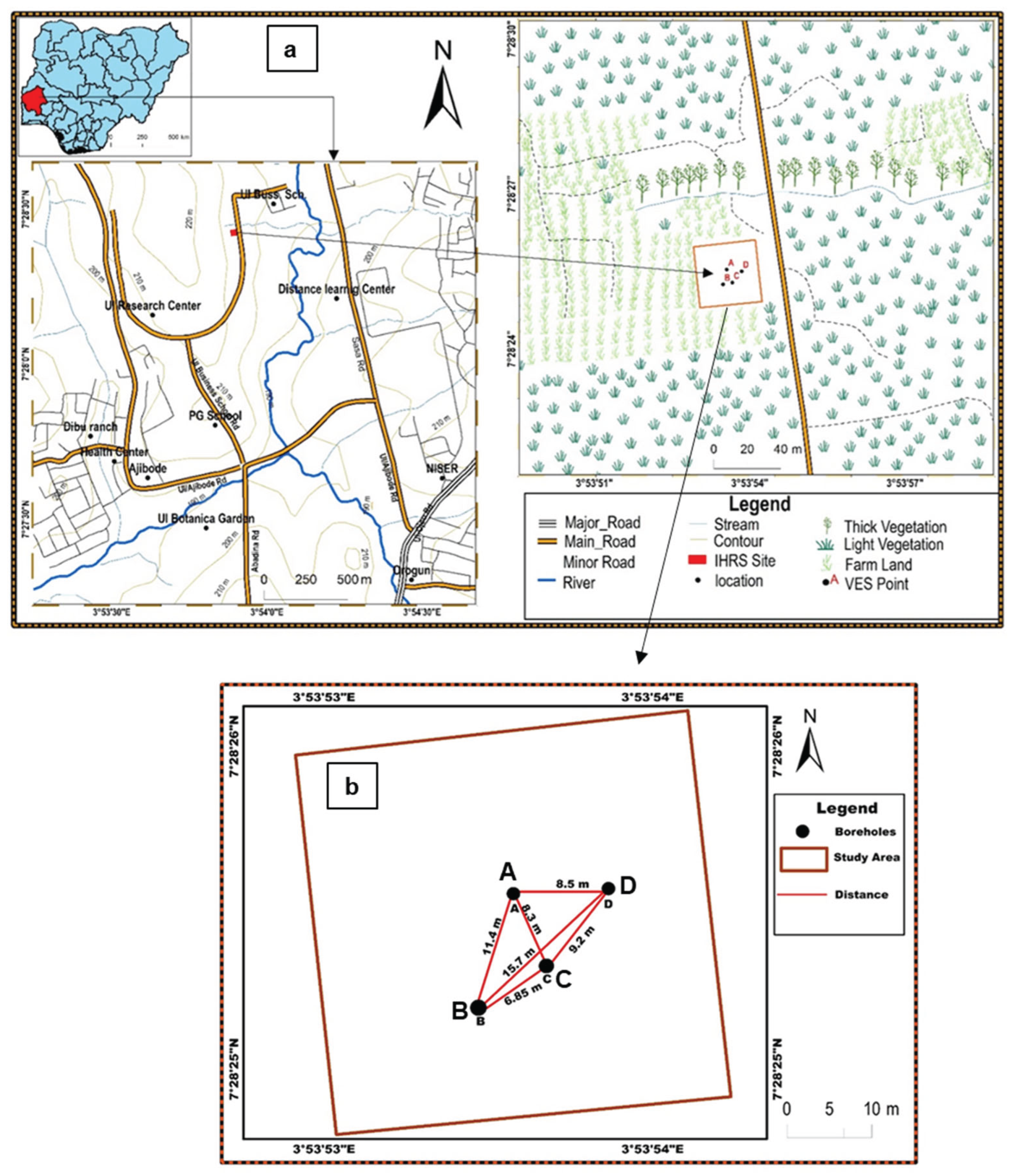
Figure 2.
Lithologic Description of the study area at Well A, B And C And D respectively. The lithologic profiles are segmented into three zones. Zone A is the top soil/sediments, zone B is the weathered zone while zone C is the fractured zone.
Figure 2.
Lithologic Description of the study area at Well A, B And C And D respectively. The lithologic profiles are segmented into three zones. Zone A is the top soil/sediments, zone B is the weathered zone while zone C is the fractured zone.
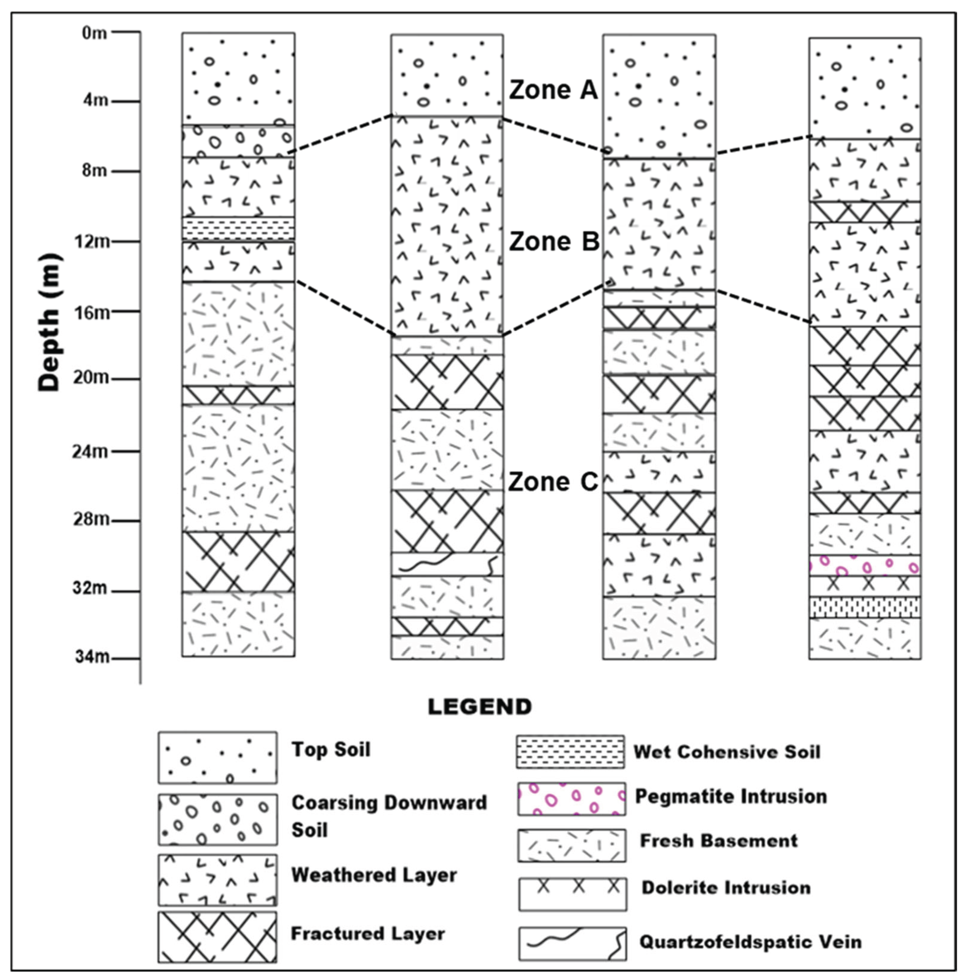
Figure 3.
Linear (column 1), semi-log (column 2) and log-log (column 3) plots of Drawdown wih time while pumping from wells A (Row 1), B (Row 2), C (Row 3) and D (Row 4). Pumping lasted for 12 hours at a constant rate of 0.9 l/s. Well drawdown-time data are presented in different colors, with blue for well A, red for well B, green for well C, and black for well D.
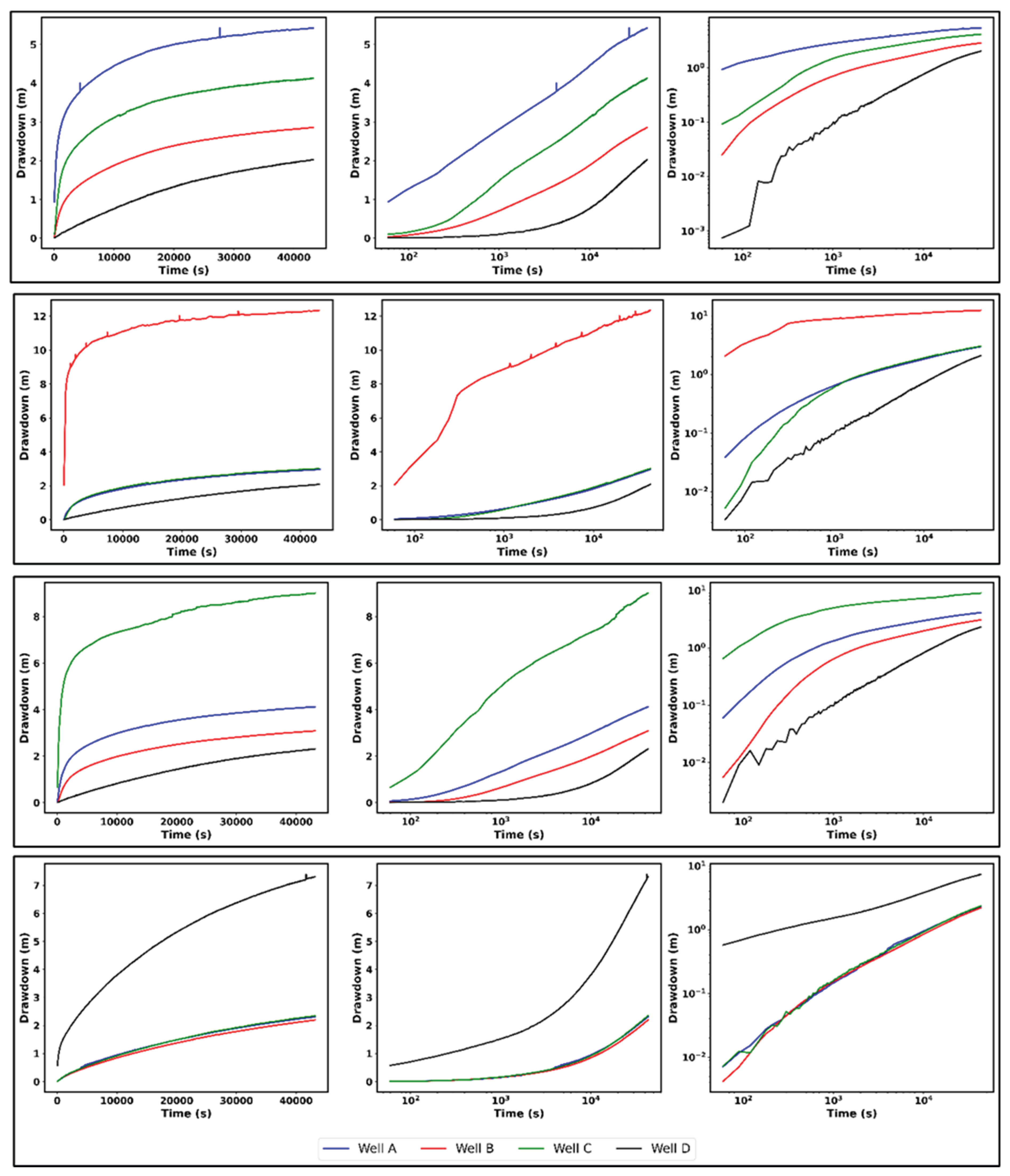
Figure 4.
Drawdown against time plot of well A while pumping at well D on a log-log scale (a) and on a semi-log scale (b) representative of a permeable fractured aquifer with a permeable medium as represented by Kruseman & de Ridder [33].
Figure 4.
Drawdown against time plot of well A while pumping at well D on a log-log scale (a) and on a semi-log scale (b) representative of a permeable fractured aquifer with a permeable medium as represented by Kruseman & de Ridder [33].
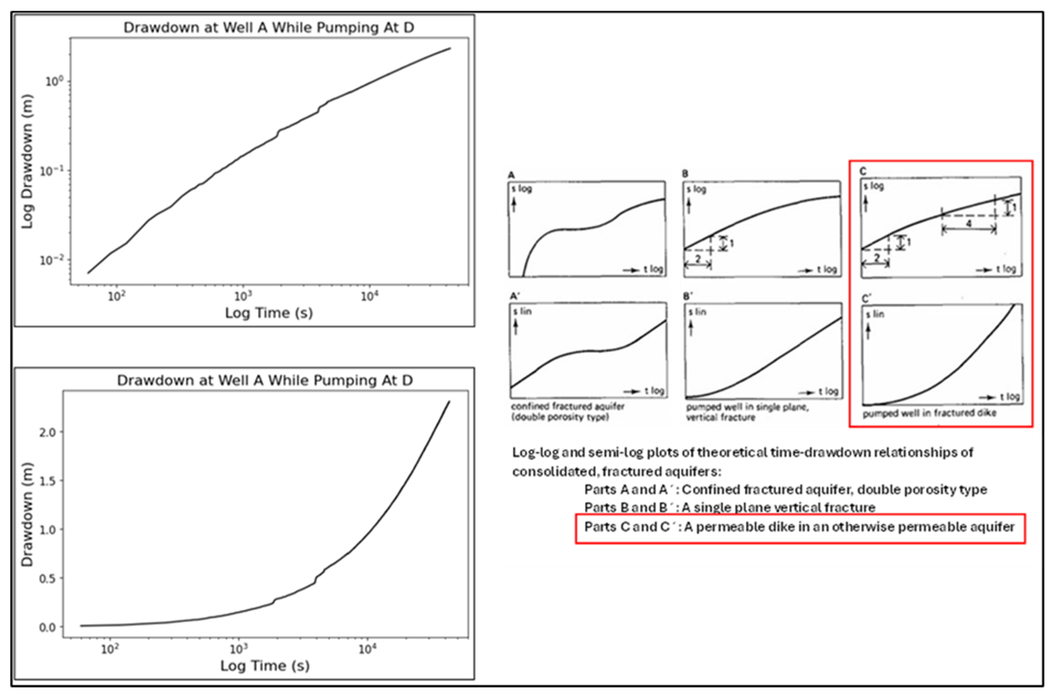
Figure 5.
Well bore storage on a log-log scale derivative plot of well B (a) and double porosity signature on a log-log scale derivative plot of well D (b) in relation to a typical derivative plot by Tonder 2001 (c) on the right.
Figure 5.
Well bore storage on a log-log scale derivative plot of well B (a) and double porosity signature on a log-log scale derivative plot of well D (b) in relation to a typical derivative plot by Tonder 2001 (c) on the right.
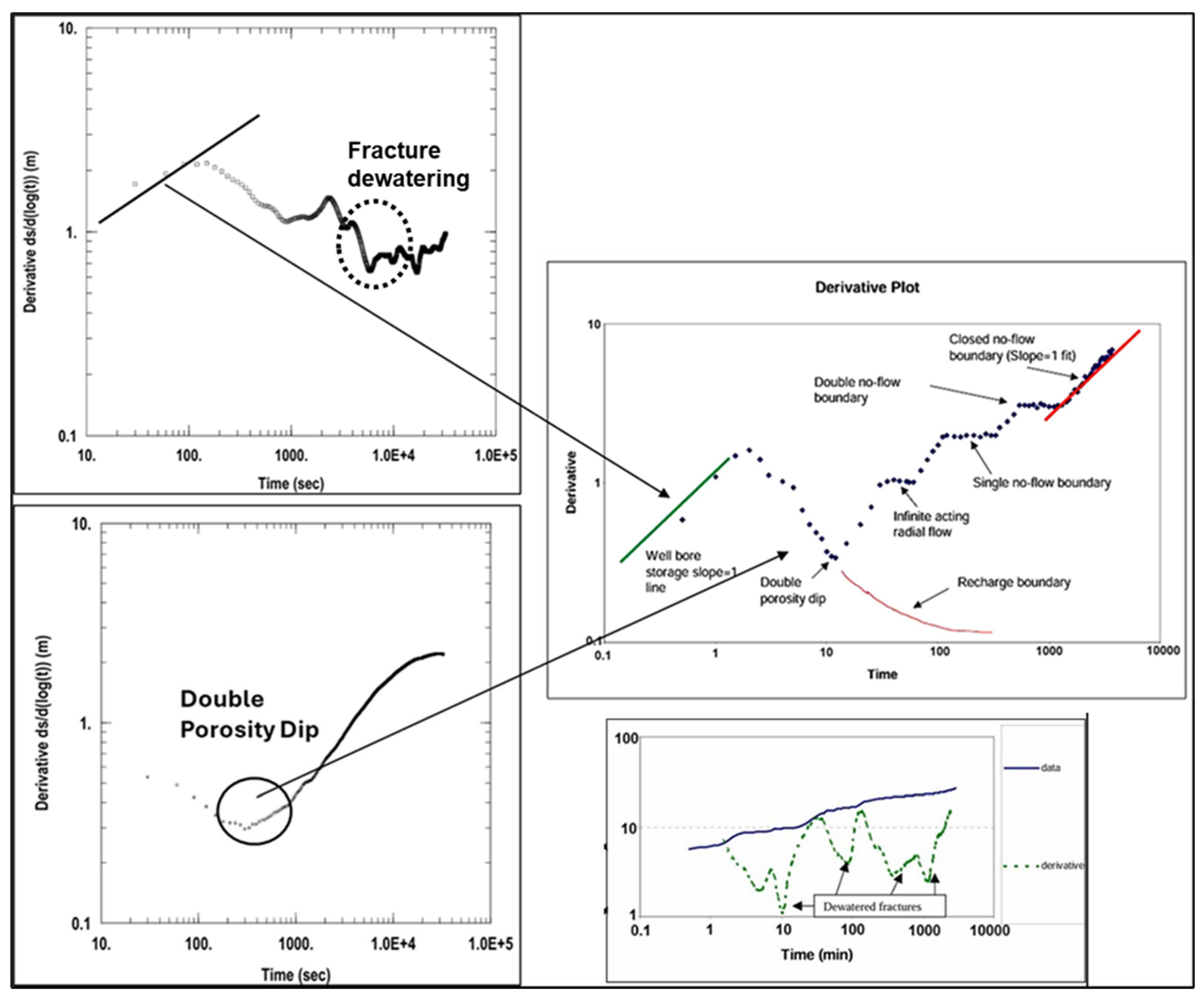
Figure 6.
Drawdown displacement and derivative curve of well C while pumping at well A fitted with the Bakers analytical solution on a semi-log scale (a) and the drawdown displacement and derivative curve of well C (pumping well) fitted with the Bakers analytical solution on a log-log scale.
Figure 6.
Drawdown displacement and derivative curve of well C while pumping at well A fitted with the Bakers analytical solution on a semi-log scale (a) and the drawdown displacement and derivative curve of well C (pumping well) fitted with the Bakers analytical solution on a log-log scale.
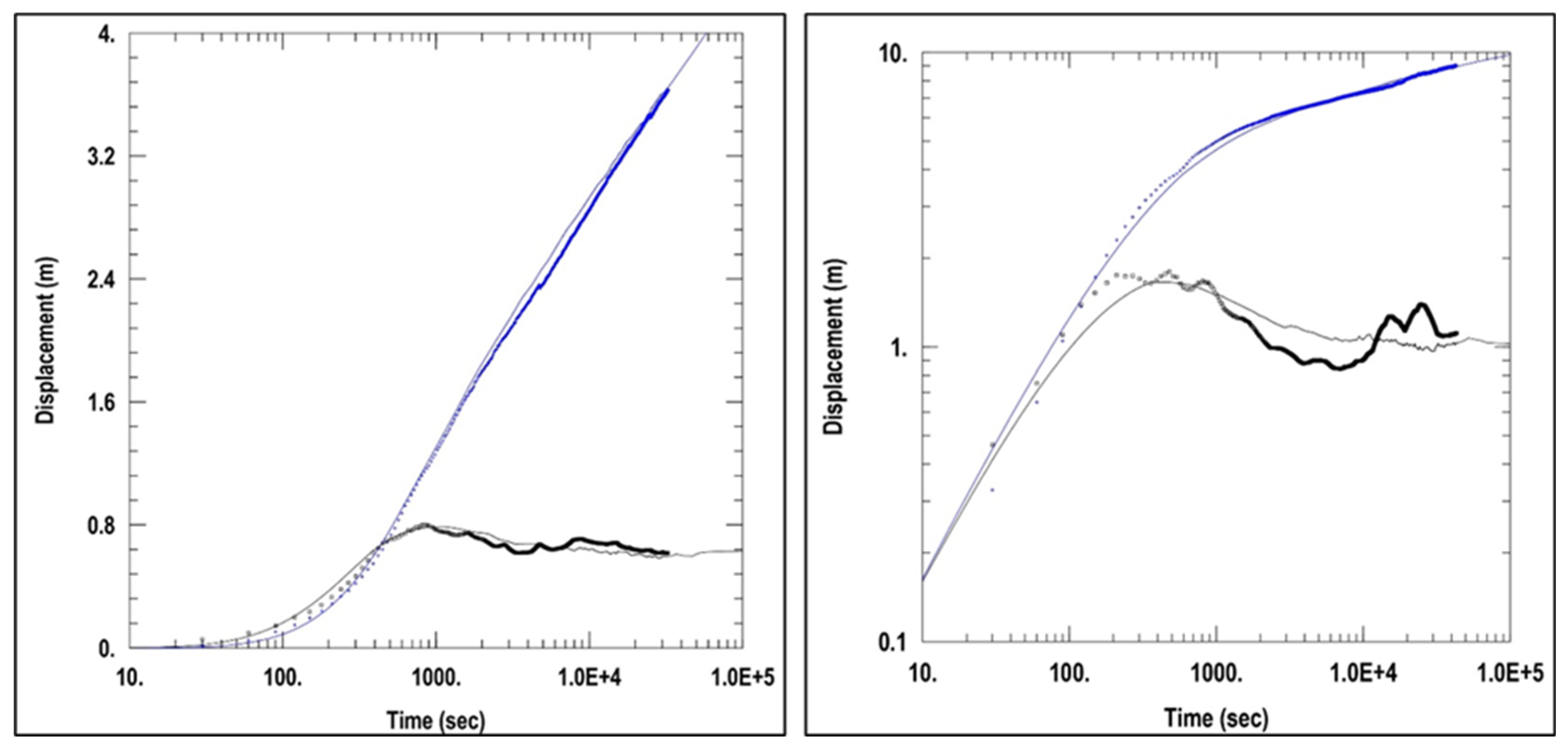
Figure 7.
Drawdown against time on a linear, semi-log, and log-log scale for wells A, B, C, and D while pumping at well C (a) and while pumping at well D (b) during the 12 hours step drawdown test.
Figure 7.
Drawdown against time on a linear, semi-log, and log-log scale for wells A, B, C, and D while pumping at well C (a) and while pumping at well D (b) during the 12 hours step drawdown test.
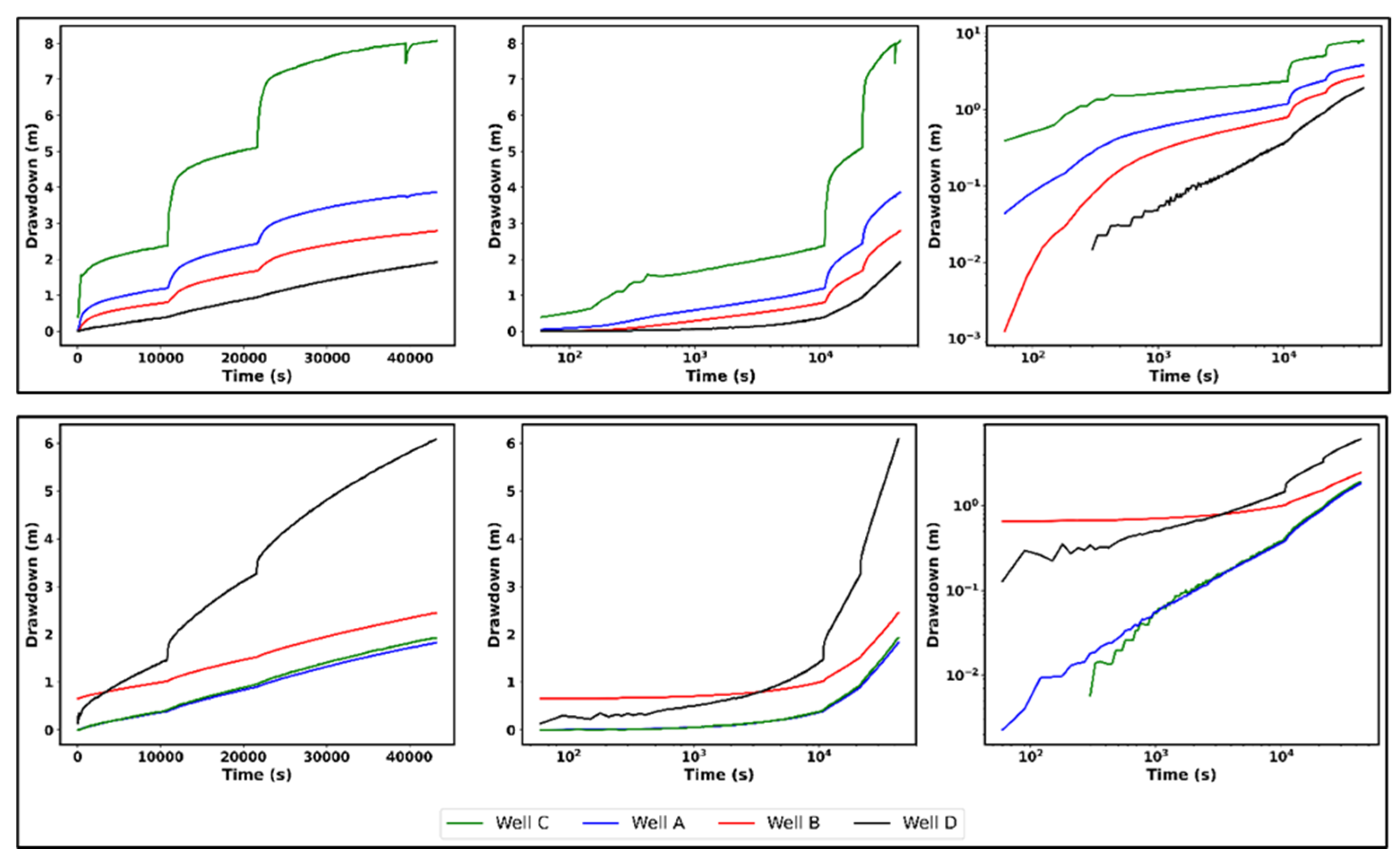
Figure 8.
Showing step drawdown displacement curve of well A while pumping at well D fitted with the Bakers analytical solution on a semi-log scale (a) and the step drawdown displacement of well D (pumping well) fitted with the Bakers analytical solution on a log-log scale.
Figure 8.
Showing step drawdown displacement curve of well A while pumping at well D fitted with the Bakers analytical solution on a semi-log scale (a) and the step drawdown displacement of well D (pumping well) fitted with the Bakers analytical solution on a log-log scale.
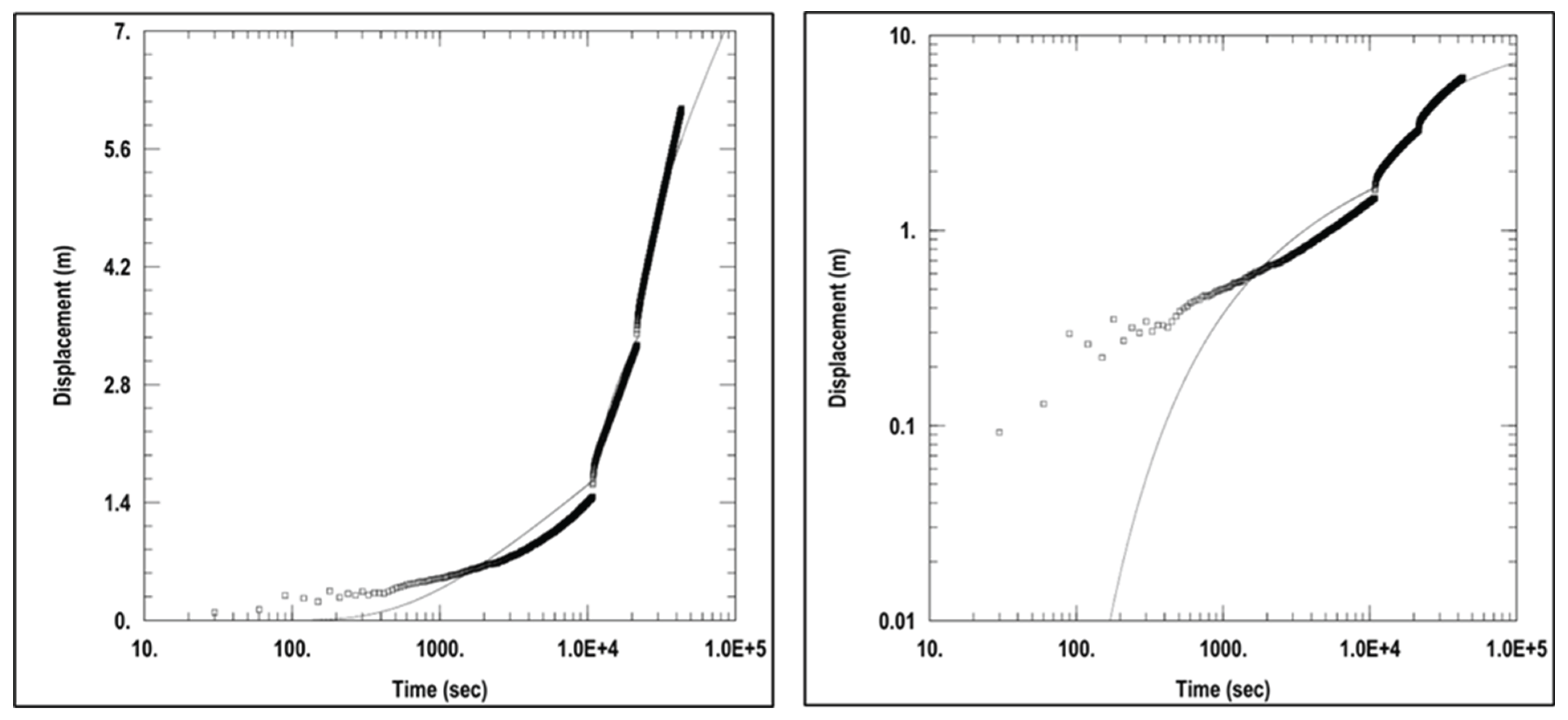
Figure 9.
Recovery in well A,B,C and D after pumping from well A (a) and after pumping from well D (b).
Figure 9.
Recovery in well A,B,C and D after pumping from well A (a) and after pumping from well D (b).
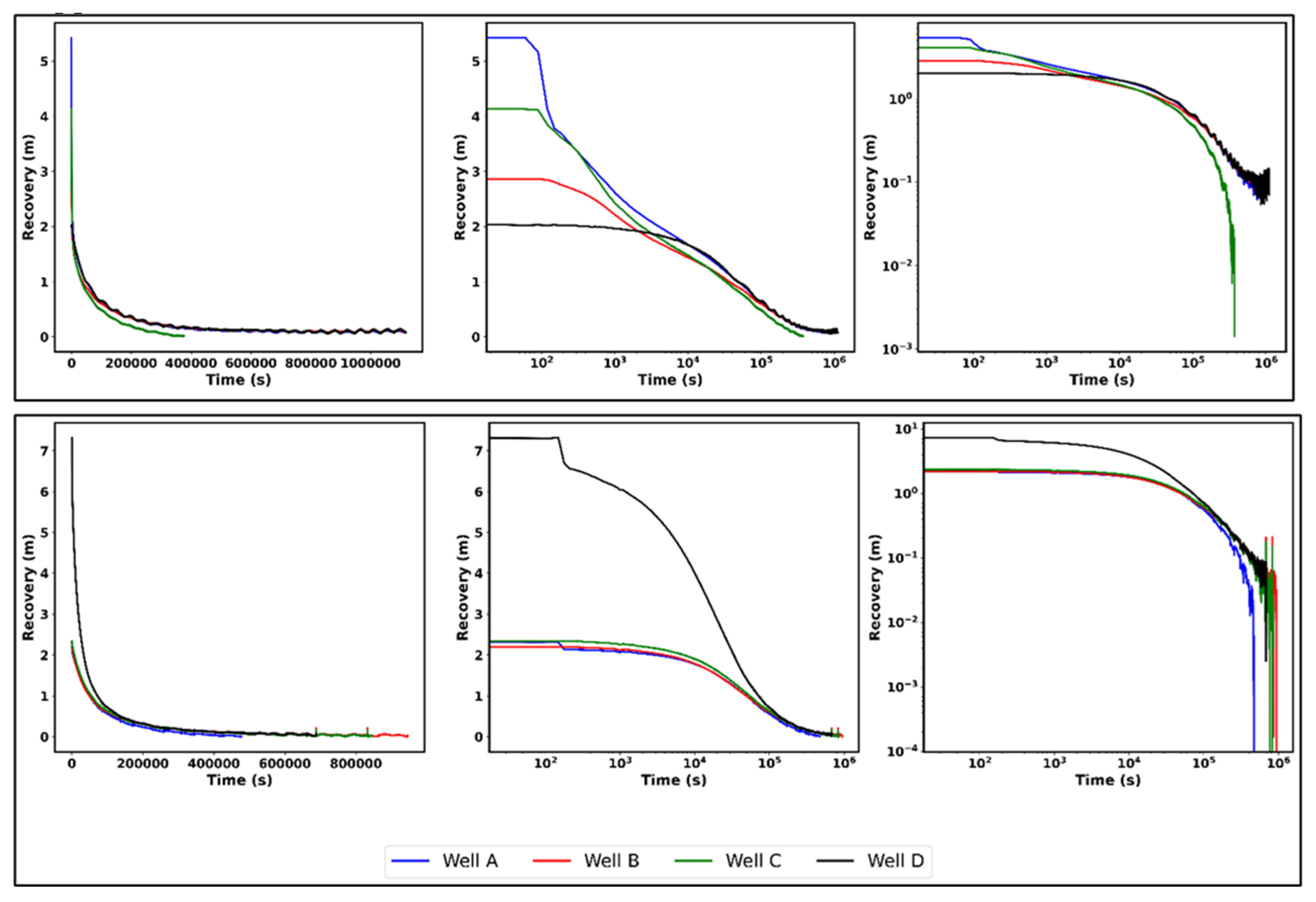
Figure 10.
Linear plots of electrical conductivity (mS/cm) against time measured at (A) the injection well and (B) the extraction well. In (C) the black line shows the estimated tracer concentration in g/L over time in the extraction well A while the orange line shows the best model fit. The blue line shows the percentage of recovered tracer. Conversion from water electrical conductivity in mS/cm to salinity in g/L relied on a linear relationship between electrical conductivity and salinity.
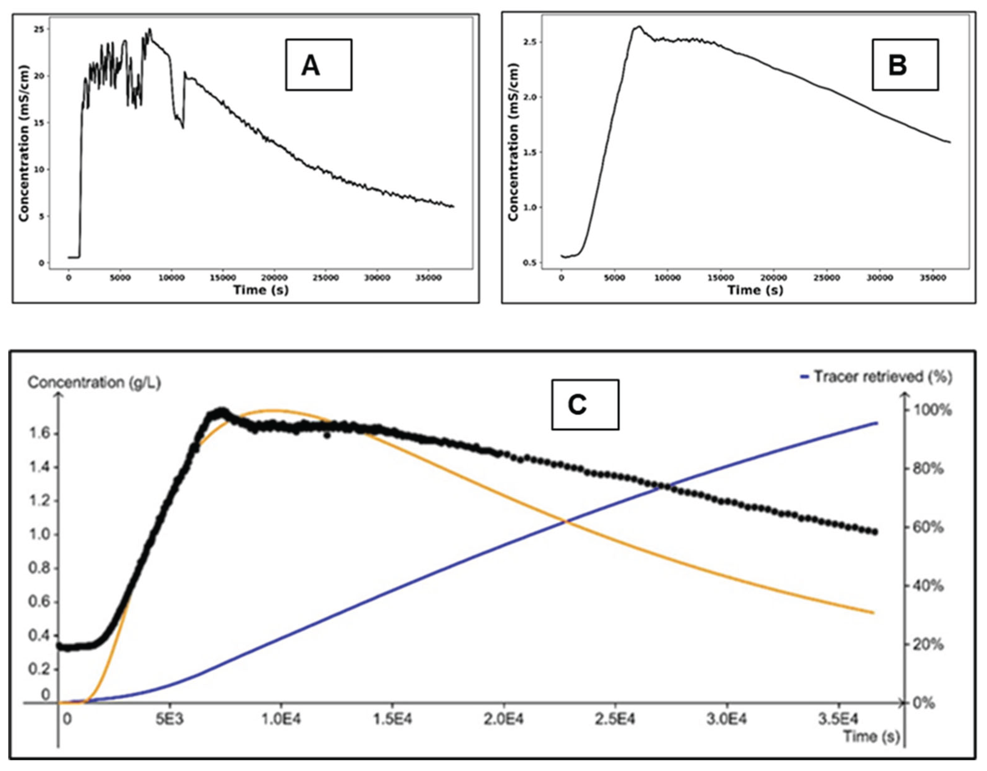

Table 1.
Drawdown observation across all wells during the 9-hour and 12-hour pumping tests.
| Well Name | Status | Distance from Pumped Well (m) | 9hrs Drawdown (m) | 12hrs Drawdown (m) |
|---|---|---|---|---|
| A | Pumping | 0 | 4.94 | 5.43 |
| B | Observation | 11.4 | 2.48 | 2.86 |
| C | Observation | 8.3 | 3.63 | 4.13 |
| D | Observation | 8.5 | 1.63 | 2.03 |
| A | Observation | 11.4 | 2.73 | 2.96 |
| B | Pumping | 0 | 12.47 | 12.58 |
| C | Observation | 6.85 | 2.68 | 3.01 |
| D | Observation | 15.7 | 1.73 | 2.08 |
| A | Pumping | 8.3 | 3.52 | 4.12 |
| B | Pumping | 6.85 | 2.55 | 3.08 |
| C | Observation | 0 | 7.22 | 9.00 |
| D | Observation | 9.2 | 1.28 | 2.31 |
| A | Observation | 8.5 | 1.77 | 2.31 |
| B | Observation | 15.7 | 1.74 | 2.19 |
| C | Observation | 9.2 | 1.86 | 2.34 |
| D | Observation | 0 | 6.18 | 7.3 |
Table 2.
Estimated Aquifer Parameters in both 9 and 12 hours Pumping Test.
| WELLS | HYDRAULIC PARAMETERS | Pumping At Well A (9 Hrs) | Pumping At Well D (9 Hrs) | Pumping At Well C (9 Hrs) | Pumping At Well B (9 Hrs) | Pumping At Well B (12 Hrs) | Pumping At Well C (12 Hrs) | Pumping At Well D (12 Hrs) | Pumping At Well A (12 Hrs) |
|---|---|---|---|---|---|---|---|---|---|
| WELL A | Fracture Hydraulic Conductivity (m/s) | 6.57E-06 | 1.23E-06 | 2.43E-06 | 2.97E-06 | 2.99E-06 | 3.22E-06 | 6.41E-07 | 1.00E-05 |
| Matrix Hydraulic Conductivity (m/s) | 1.09E-06 | 1.92E-09 | 2.43E-10 | 3.54E-10 | 3.40E-10 | 2.61E-10 | 1.00E-10 | 1.00E-10 | |
| Fracture Specific Storage (m-1) | 2.46E-04 | 2.30E-06 | 2.77E-07 | 3.03E-07 | 3.15E-07 | 2.14E-07 | 1.96E-06 | 1.08E-04 | |
| Matrix Specific Storage (m-1) | 5.48E-02 | 9.75E-04 | 7.33E-05 | 6.88E-05 | 6.53E-05 | 2.42E-05 | 4.85E-03 | 7.02E-05 | |
| Transmissivity (m²/s) | 1.01E-04 | 1.89E-05 | 3.71E-05 | 4.54E-05 | 4.56E-05 | 4.92E-05 | 9.79E-06 | 1.54E-04 | |
| Flow Dimension (n) | 2.055 | 2.22 | 1.972 | 2 | 2 | 2 | 2 | 1.776 | |
| WELL B | Fracture Hydraulic Conductivity (m/s) | 3.82E-06 | 3.64E-06 | 2.64E-06 | 3.53E-06 | 3.54E-06 | 3.17E-06 | 7.85E-07 | 1.66E-05 |
| Matrix Hydraulic Conductivity (m/s) | 9.19E-10 | 4.29E-08 | 6.95E-10 | 7.69E-10 | 1.00E-10 | 7.63E-10 | 1.00E-10 | 4.25E-02 | |
| Fracture-Specific Storage | 5.78E-07 | 5.07E-05 | 2.06E-05 | 4.60E-06 | 1.09E-06 | 1.89E-05 | 6.35E-07 | 4.51E-05 | |
| Matrix Specific Storage | 9.19E-05 | 1.16E-04 | 2.23E-04 | 1.00E-10 | 1.00E-10 | 1.20E-04 | 5.40E-04 | 1.16E-10 | |
| Transmissivity (m²/s) | 1.06E-04 | 1.01E-04 | 7.30E-05 | 9.75E-05 | 9.77E-05 | 8.70E-05 | 2.17E-05 | 2.53E-04 | |
| Flow Dimension (n) | 2.352 | 1.996 | 2 | 2 | 2 | 2 | 2 | 1.712 | |
| WELL C | Fracture Hydraulic Conductivity (m/s) | 7.19E-06 | 1.91E-06 | 2.76E-06 | 3.71E-06 | 1.82E-06 | 2.49E-06 | 1.45E-05 | 2.66E-06 |
| Matrix Hydraulic Conductivity (m/s) | 1.87E-10 | 8.06E-09 | 7.67E-09 | 1.43E-09 | 1.45E-10 | 1.00E-10 | 6.14E-02 | 1.00E-10 | |
| Fracture-Specific Storage | 1.16E-05 | 1.29E-05 | 1.90E-03 | 2.24E-05 | 1.70E-05 | 2.46E-03 | 1.95E-04 | 3.02E-06 | |
| Matrix Specific Storage | 1.30E-05 | 4.94E-04 | 9.31E-04 | 7.84E-05 | 5.65E-04 | 1.00E-10 | 1.00E-10 | 1.43E-04 | |
| Transmissivity (m²/s) | 1.99E-04 | 5.30E-05 | 7.66E-05 | 1.03E-04 | 5.05E-05 | 6.91E-05 | 4.03E-04 | 4.06E-05 | |
| Flow Dimension (n) | 2 | 2 | 2 | 2.05 | 2 | 2 | 0.9255 | ||
| WELL D | Fracture Hydraulic Conductivity (m/s) | 2.63E-07 | 5.11E-07 | 5.59E-08 | 5.50E-06 | 1.36E-06 | 4.36E-07 | 4.80E-07 | 1.64E-05 |
| Matrix Hydraulic Conductivity (m/s) | 3.52E-10 | 1.00E+00 | 1.71E-10 | 6.70E-05 | 1.00E-10 | 1.13E-10 | 4.04E-01 | 1.42E-05 | |
| Fracture-Specific Storage | 1.27E-05 | 1.25E+00 | 1.90E-06 | 1.00E-03 | 1.12E-06 | 1.86E-06 | 1.10E+00 | 2.40E-03 | |
| Matrix Specific Storage | 1.02E-02 | 1.00E+00 | 3.34E-03 | 1.00E-03 | 5.44E-04 | 2.48E-03 | 9.54E-01 | 2.83E-08 | |
| Transmissivity (m²/s) | 7.28E-06 | 1.41E-05 | 1.54E-06 | 1.52E-04 | 3.75E-05 | 1.21E-05 | 1.33E-05 | 1.64E-05 | |
| Flow Dimension (n) | 2.676 | 2 | 2 | 2 | 2 | 2 | 2 |
Table 3.
Specific yield at various distances of the monitoring well to the extraction during the 12 hours pumping exercise.
Table 3.
Specific yield at various distances of the monitoring well to the extraction during the 12 hours pumping exercise.
| Pumping Well | Extraction Well | A | B | C | D |
| A | Specific Yield (%) | 0.16% | 0.22% | 0.34% | |
| Distance from pumping well | 11.4 m | 8.3 m | 8.5 m | ||
| Volume of material dewatered (m³) | 3426.8 m³ | 2427.6 m³ | 1575.9 m³ | ||
| Volume of water drained (Liters) | 38.84 L | 53.41 L | 53.58 L | ||
| B | Specific Yield (%) | 0.03% | 0.08% | 0.05% | |
| Distance from pumping well | 11.4 m | 6.85 m | 15.7 m | ||
| Volume of material dewatered (m³) | 16358.75 m³ | 6295.01 m³ | 9494.89 m³ | ||
| Volume of water drained (Liters) | 50.71 L | 50.36 L | 47.48 L | ||
| C | Specific Yield (%) | 0.04% | 0.17% | 0.20% | |
| Distance from pumping well | 8.3 m | 6.85 m | 9.2 m | ||
| Volume of material dewatered (m³) | 12448.4 m³ | 3075.7 m³ | 2595.83 m³ | ||
| Volume of water drained (Liters) | 49.794 L | 52.29 L | 51.926 L | ||
| D | Specific Yield (%) | 0.28% | 0.08% | 0.24% | |
| Distance from pumping well | 8.5 m | 15.7 m | 9.2 m | ||
| Volume of material dewatered (m³) | 1906.7 m³ | 6372.93 m³ | 2247.88 m³ | ||
| Volume of water drained (Liters) | 53.38 L | 50.98 L | 53.94 L |
Table 4.
Estimated Sustainable Yield of Each Well using FC-Method.
| Well | Sustainable Yield | Number of Persons That can be supplied |
| A | 1166.4 m³ at 0.45 L/s | 1555 People |
| B | 414.72 m³ at 0.16 L/s | 553 People |
| C | 803.52 m³ at 0.31 L/s | 1071 People |
| D | 984.96 m³ at 0.38 L/s | 1313 People |
Disclaimer/Publisher’s Note: The statements, opinions and data contained in all publications are solely those of the individual author(s) and contributor(s) and not of MDPI and/or the editor(s). MDPI and/or the editor(s) disclaim responsibility for any injury to people or property resulting from any ideas, methods, instructions or products referred to in the content. |
© 2025 by the authors. Licensee MDPI, Basel, Switzerland. This article is an open access article distributed under the terms and conditions of the Creative Commons Attribution (CC BY) license (http://creativecommons.org/licenses/by/4.0/).
Copyright: This open access article is published under a Creative Commons CC BY 4.0 license, which permit the free download, distribution, and reuse, provided that the author and preprint are cited in any reuse.


