Submitted:
13 May 2025
Posted:
14 May 2025
You are already at the latest version
Abstract
The increasing deployment of complex machine learning models in high-stakes financial applications, such as asset pricing, credit risk assessment, and fraud detection, has heightened the demand for model explainability. Feature attribution methods are commonly employed to provide insights into model decisions by assigning importance scores to input features. However, these attributions are often misconstrued as indicators of true causal influence, a leap that can be particularly perilous in finance where spurious correlations and confounding variables are prevalent. This paper investigates the causal faithfulness of various feature attribution methods using finance-motivated synthetic data-generating processes with known causal ground truths for asset pricing, credit risk, and fraud detection. We train Multilayer Perceptrons, LSTMs, and XGBoost models and evaluate the ability of attribution methods (including SHAP, Integrated Gradients, and XGBoost's built-in importance) to identify causal features. Our experiments show that XGBoost's built-in feature importance provides the most causally faithful explanations overall, and XGBoost models generally yield more causally accurate attributions across scenarios. Asset pricing was the best-performing scenario for causal feature identification based on overall faithfulness scores with top methods. However, fraud detection presents unique challenges, where indirect indicators (consequences of fraud) often receive substantial attribution weight despite not being causal drivers. Significant variability in performance across methods suggests using multiple techniques for robust understanding. These findings underscore the critical need for practitioners to exercise caution when interpreting feature attributions as causal explanations, emphasizing the necessity of domain expertise and proper validation.
Keywords:
xgboost
; finance
; xai
1. Introduction
The financial industry has witnessed a rapid adoption of sophisticated machine learning (ML) models, particularly “black-box” algorithms like deep neural networks and gradient boosting machines. These models are increasingly utilized for critical tasks such as algorithmic trading, asset pricing, credit scoring, risk management, and fraud detection [1]. While their predictive power can be substantial, their inherent complexity often obscures the reasoning behind their decisions, leading to a “black-box” problem.
1.1. Problem Statement
This lack of transparency poses significant challenges. Regulatory bodies worldwide are progressively demanding greater explainability and accountability for automated financial systems (e.g., GDPR’s “right to explanation,” SR 11-7 in the US). Beyond compliance, financial institutions themselves require a deeper understanding of model behavior to manage risks, ensure fairness, build trust, and refine strategies. Feature attribution methods have emerged as a popular approach to peer inside these black boxes by assigning importance scores to input features based on their contribution to a model’s output.
However, a critical gap exists: feature attributions are often implicitly or explicitly interpreted as indicators of causal relationships. Stakeholders may assume that a highly attributed feature is a “driver” or “cause” of the predicted outcome. This leap from attributional importance to causal importance is not inherently guaranteed and can be misleading, especially in finance. Financial systems are characterized by complex interdependencies, strong confounding effects (e.g., market-wide sentiment), prevalent spurious correlations, and the use of proxy variables that may inadvertently capture sensitive information.
1.2. Research Objectives
This paper aims to rigorously evaluate the faithfulness of commonly used feature attribution methods as causal explanations, specifically within simulated financial contexts. Our primary objectives are:
- 1)
- To assess how well different attribution techniques (e.g., gradient-based, SHAP, XGBoost built-in) identify the true causal features versus non-causal (spurious or confounded) features in financial ML models.
- 2)
- To design and implement synthetic data-generating processes that mirror plausible causal structures found in three key financial scenarios: asset pricing, credit risk assessment, and fraud detection.
- 3)
- To identify specific scenarios and causal structures where current attribution methods are most likely to provide misleading or causally unfaithful explanations.
- 4)
- To provide insights and potential guidelines for financial practitioners on the cautious interpretation of feature attributions and the importance of considering underlying causal assumptions.
1.3. Significance in Financial Domain
The implications of causally unfaithful explanations in finance are profound:
- Investment Strategies: Misattributing market movements to spurious indicators rather than true economic drivers can lead to flawed investment strategies and capital misallocation.
- Credit Risk and Fairness: If a credit scoring model attributes risk to a feature that is merely a proxy for a protected attribute (e.g., race or gender) due to socioeconomic confounding, it can perpetuate and amplify biases, leading to unfair lending decisions.
- Fraud Detection: Mistaking consequences of fraud for its causes can lead to reactive rather than proactive fraud prevention measures, and potentially misdirect investigative efforts.
- Regulatory Compliance and Model Auditing: Regulators require transparent and fair models. If the explanations provided are not causally sound, institutions may fail to meet these requirements or, worse, mask problematic model behavior.
- Systemic Risk: A widespread reliance on models whose explanations are causally flawed could, in aggregate, contribute to systemic misjudgments of risk or market dynamics.
By systematically investigating these “causal pitfalls,” this research seeks to foster a more nuanced understanding of the capabilities and limitations of feature attribution methods in finance, contributing to the development of more robust and truly explainable AI systems for this critical domain.
2. Literature Review
The pursuit of interpretable machine learning, often termed Explainable AI (XAI), has gained significant traction, particularly in high-stakes domains like finance. This section reviews relevant literature in three key areas: feature attribution methods, causal inference in ML, and the application of XAI in finance.
2.1. Feature Attribution Methods
Feature attribution methods aim to quantify the contribution of each input feature to a model’s prediction for a specific instance or globally. These methods can be broadly categorized:
- Gradient-based approaches: These methods utilize the gradients of the model’s output with respect to its inputs. A simple example is Saliency Maps [2], which use the absolute value of the gradient. Extensions include Gradient×Input [3], which multiplies the gradient by the input feature value, and Integrated Gradients (IG) [4], which satisfies axioms like sensitivity and implementation invariance by integrating gradients along a path from a baseline input to the actual input.
- Perturbation-based methods: These methods assess feature importance by observing the change in model output when features are perturbed, masked, or removed. LIME (Local Interpretable Model-agnostic Explanations) [5] is a prominent example, which learns a simple, interpretable local linear model around the prediction to be explained.
- Model-specific techniques: Some methods are tailored to particular model architectures. For tree-based ensembles like XGBoost, feature importances can be derived from metrics like “gain” (total reduction in loss due to splits on a feature), “weight” (number of times a feature is used to split), or “cover” (average number of samples affected by splits on a feature). SHAP (SHapley Additive exPlanations) [6] provides a unified framework based on game-theoretic Shapley values, offering both model-specific (e.g., TreeSHAP for tree ensembles) and model-agnostic (e.g., KernelSHAP) versions. Attention mechanisms in Transformer models can also be interpreted as a form of feature attribution, though their direct interpretation as importance scores is debated [7].
- Decomposition-based methods: Layer-Wise Relevance Propagation (LRP) [8] decomposes the prediction score backwards through the network layers to assign relevance scores to inputs.
While these methods offer valuable insights into what features a model is using, they do not inherently explain why those features are causally relevant to the underlying real-world phenomenon the model is trying to capture.
2.2. Causal Inference in Machine Learning
Causal inference [9] aims to move beyond correlation to understand cause-and-effect relationships. Key concepts include:
- Directed Acyclic Graphs (DAGs): DAGs are used to represent causal assumptions among variables, where nodes are variables and directed edges represent causal influences. The absence of an edge implies no direct causal effect.
- Confounding Variables: A confounder is a variable that causally influences both the “treatment” (or feature of interest) and the “outcome” (or target variable), potentially creating a spurious correlation between them if not accounted for.
- Interventional vs. Observational Data: Observational data, common in finance, only allows us to see correlations (). Causal claims often require understanding interventional distributions (), i.e., the effect of actively changing X. ML models trained on observational data learn correlational patterns.
There’s a growing body of research at the intersection of causality and ML, focusing on areas like causal discovery, learning representations that are invariant to certain interventions [10], and evaluating explanations from a causal perspective [11]. The challenge lies in the fact that standard ML models, including those for which attributions are computed, are typically trained to optimize predictive accuracy on observational data, not to uncover causal structures.
2.3. Explainable AI in Finance
The financial sector has unique drivers for XAI:
- Regulatory Scrutiny: Regulations like the Equal Credit Opportunity Act (ECOA) in the U.S. (requiring explanations for adverse credit decisions) and GDPR in Europe necessitate model transparency.
- Risk Management: Understanding model vulnerabilities, potential biases, and behavior under stress is crucial for internal risk control.
- Stakeholder Trust: Explanations can help build trust with clients, investors, and internal users.
- Model Debugging and Improvement: Interpretability aids in identifying model flaws and improving performance.
Current applications of XAI in finance involve using methods like SHAP and LIME to explain predictions from models used in credit scoring, fraud detection, algorithmic trading, and customer analytics [1]. However, the focus is often on “model-true” explanations (what the model learned) rather than “data-true” or “world-true” explanations (how the real-world system behaves causally). This paper specifically addresses the gap by evaluating if model-true attributions align with world-true causal relationships in financial settings. The inherent noise, non-stationarity, and complex feedback loops in financial data make this a particularly challenging but critical area of inquiry.
3. Theoretical Framework
The core premise of this paper is that feature attributions derived from machine learning models, while indicative of feature importance for the model’s prediction, may not align with the true causal influence of those features on the real-world outcome. This discrepancy is particularly acute in finance due to the inherent characteristics of financial data and systems.
3.1. Causal Structures in Financial Data
Financial systems are complex, dynamic, and rife with structures that can mislead purely correlational learning algorithms and, consequently, their attribution-based explanations.
-
Confounding Variables: These are ubiquitous in finance.
- Market-wide factors: Broad market sentiment, macroeconomic announcements (e.g., interest rate changes, inflation reports), geopolitical events, or even unobserved liquidity shocks can influence both individual asset prices (or other financial outcomes) and various observable features used by models. For example, strong positive market sentiment (Z) might simultaneously boost a stock’s price (Y) and increase trading volume () for that stock. A model might attribute predictive power to for Y, even if volume itself isn’t a direct cause, because both are driven by Z.
- Sector-specific effects: News or trends affecting an entire industry can act as confounders for individual company performance and related features.
- Socioeconomic factors in credit/fraud: In credit risk, variables like local unemployment rates or economic downturns (Z) can affect both an individual’s financial behavior (e.g., payment history, ) and their likelihood of default (Y), while also correlating with proxy variables like zip code ().
-
Proxy Variables and Indirect Indicators:
- Proxy Bias: Features that are not directly causal but are correlated with protected attributes (like race, gender) and also with the outcome (e.g., default risk) due to systemic biases or socioeconomic confounding. Attribution methods might highlight these proxies, leading to interpretations that mask discrimination or misattribute risk.
- Indirect Indicators (Consequences vs. Causes): In fraud detection, some features might be strong predictors because they are consequences of fraud, not its root causes. For instance, a sudden flurry of small transactions () might occur after an account is compromised (). While is predictive, attributing fraud to it mistakes an effect for a cause.
- Spurious Correlations due to Non-Stationarity and Noise: Financial time series are often non-stationary, and the sheer volume of available data can lead to coincidental correlations that hold over certain periods but lack any underlying causal link. Models can easily overfit to such patterns, and attribution methods would then highlight these spurious features.
- Temporal Dependencies and Feedback Loops: Past outcomes can influence future features and outcomes, creating complex feedback loops that are hard to disentangle causally from purely observational data.
3.2. Attribution Methods’ Limitations in a Causal Context
Attribution methods, by their design, explain the model’s behavior, not necessarily the data-generating process of the real world.
- Correlation vs. Causation: Standard ML models are optimized to find correlational patterns that maximize predictive accuracy. If a non-causal feature is highly correlated with the target Y (perhaps due to a confounder Z), the model will likely learn to use . Attribution methods will then correctly report that is important to the model, but this can be easily misinterpreted as being causally important for Y in the real world.
- Sensitivity to Model Specification: The attributions are model-dependent. Different models, even if trained on the same data and achieving similar predictive accuracy, can learn different internal representations and thus yield different feature attributions. This makes it hard to claim a universal “causal” interpretation from model-based attributions alone.
- Local vs. Global Explanations: Methods like LIME provide local explanations. While useful for understanding a single prediction, these local attributions might not generalize to global causal statements, especially if the model’s decision boundaries are highly non-linear. Even global methods like SHAP average local effects, which might obscure context-specific causal relationships.
- Ignoring Unobserved Confounders: Attribution methods operate on the features provided to the model. If a critical unobserved confounder influences both an observed feature and the target, the observed feature might receive high attribution, masking the true causal role of the unobserved variable.
- Baseline Choice (for methods like Integrated Gradients): The choice of baseline for path-based attribution methods can significantly affect the resulting scores, and defining a causally meaningful baseline is non-trivial, especially for complex, high-dimensional financial data.
This theoretical framework suggests that while feature attributions are valuable tools for model debugging and understanding learned patterns, their direct use as causal explanations in finance is fraught with peril. This study empirically tests these limitations using synthetic data where the causal ground truth is known.
4. Methodology
To empirically evaluate the causal faithfulness of feature attribution methods in financial contexts, we adopt a methodology centered around synthetic data generation with known causal ground truths, diverse model training, and the application of various attribution techniques.
4.1. Synthetic Data Generation
We designed three distinct financial scenarios, each represented by a Directed Acyclic Graph (DAG) that defines the causal relationships between latent confounders (Z), causal features (), non-causal/spurious features (), and the target variable (Y). The number of causal features was typically 2, with 2-3 non-causal features (spurious or indirect) and 2 confounding variables.
4.1.1. Asset Pricing Scenario
- Objective: Predict future stock returns (regression task).
- Features: Causal features (e.g., fundamental_0, fundamental_1) represent true economic drivers. Spurious features (e.g., spurious_0, spurious_1, spurious_2) are correlated with returns via common confounders (e.g., market sentiment) but are not direct causes.
4.1.2. Credit Risk Scenario
- Objective: Predict loan default probability (binary classification task).
- Features: Causal features (e.g., behavioral_0, behavioral_1) represent true behavioral risk factors. Proxy features (e.g., proxy_0, proxy_1) are non-causal but may be correlated with default through socioeconomic confounders, potentially capturing biases.
4.1.3. Fraud Detection Scenario
- Objective: Identify fraudulent transactions (imbalanced binary classification task).
- Features: Causal features (e.g., anomaly_0, anomaly_1) represent true indicators of fraudulent activity. Indirect indicators (e.g., indirect_0, indirect_1) are consequences of fraud (e.g., subsequent account lock) and are thus highly predictive but not causal drivers.
For each scenario, feature data and target data were generated, along with information identifying the true causal features.
4.2. Model Architectures
We employed a range of models commonly used in financial applications:
- Multilayer Perceptrons (MLPs): Standard feedforward neural networks.
- Long Short-Term Memory Networks (LSTMs): Intended for sequential data but applied to tabular data by treating samples as sequences.
- Gradient Boosting Machines (XGBoost): Utilizing the XGBoost library, known for strong performance on tabular data.
All models were trained for each scenario using appropriate loss functions.
4.3. Attribution Methods to Evaluate
We evaluated several feature attribution methods:
- Saliency Maps: Gradient-based.
- Gradient × Input: Modified gradient-based.
- Integrated Gradients (IG): Path-integral based gradient method.
- SHAP (SHapley Additive exPlanations): Game-theoretic approach, using TreeSHAP for XGBoost models.
- XGBoost Built-in Feature Importance (denoted ’xgboost’ in results): Native feature importance scores from XGBoost models (based on ’gain’).
This paper provides a comprehensive analysis of these methods, with particular attention to the performance of XGBoost’s built-in importance and SHAP due to their prominence and the study’s findings.
5. Experimental Design
Our experimental design focuses on systematically training models on the synthetic datasets, applying various attribution methods, and then evaluating the causal faithfulness of these attributions using predefined metrics.
5.1. Evaluation Metrics for Causal Faithfulness
We assess whether attribution methods assign higher importance to true causal features compared to non-causal ones.
-
Attribution Ranking Metrics:
- Top-K Accuracy: Proportion of the top k attributed features (where k is the true number of causal features) that are indeed causal. Higher is better.
-
Attribution Magnitude Metrics:
- Attribution Ratio: Ratio of mean absolute attribution of causal features to non-causal features. Higher values indicate better discrimination.
- Overall Faithfulness Score: A composite score combining several normalized key metrics. Less negative values (closer to zero) are better.
5.2. Benchmark Scenarios and Experimental Protocol
The protocol involved:
- Generating datasets for the three financial scenarios.
- Training MLP, LSTM, and XGBoost models on each scenario.
- Computing feature attributions using Saliency, Gradient×Input, Integrated Gradients, SHAP, and XGBoost built-in importance for the trained models (primarily XGBoost models in detailed analysis).
- Evaluating causal faithfulness using the metrics defined above and generating visualizations.
Experiments varied the financial scenario, model type, and attribution method. A fixed random seed (42) was used for reproducibility.
6. Results and Analysis
This section presents key results, focusing on XGBoost models due to their strong predictive performance and the clear patterns observed in their attributions.
6.1. Model Performance
Table 1 summarizes the predictive performance. XGBoost models generally exhibited the strongest performance across scenarios, particularly in classification tasks, achieving high F1 scores and accuracy. For instance, in asset pricing, XGBoost achieved an R² of 0.9543, and in fraud detection, an F1 score of 0.9561.
6.2. Faithfulness Evaluation: Attribution Method Comparison
Table 2 shows a summary of performance for different attribution methods applied to XGBoost models, averaged across the three scenarios. XGBoost’s built-in feature importance (denoted ’xgboost’) demonstrated the highest Overall Faithfulness Score (-29.6574) and perfect Top-K Accuracy (1.0000). SHAP also performed strongly, with an Overall Score of -29.6700 and Top-K Accuracy of 0.9837. Gradient-based methods (Saliency, Gradient×Input, Integrated Gradients) showed considerably lower performance on these metrics, with Top-K Accuracies around 0.4710.
Figure 1 visualizes the overall faithfulness scores for XGBoost models across attribution methods and scenarios. Asset pricing consistently shows better (less negative) scores, especially for the ’xgboost’ and ’shap’ attribution methods. Figure 2 and Figure 3 provide bar chart comparisons, illustrating the superior performance of ’xgboost’ and ’shap’ methods in terms of overall score and Top-K accuracy, respectively, across all scenarios compared to gradient-based methods.
6.3. Scenario-Specific Analysis (XGBoost Model)
We detail performance for the XGBoost model, highlighting its built-in ’xgboost’ attribution method and SHAP.
6.3.1. Asset Pricing
The best overall performance combination was the XGBoost model with its ’xgboost’ attribution method in the Asset Pricing scenario.
-
XGBoost model, ’xgboost’ method:
- –
- Overall Faithfulness Score: -24.0987
- –
- Top-K Accuracy: 1.0000
- –
- Attribution Ratio (Causal/Non-Causal): 7.4218
Figure 4 shows that XGBoost’s built-in importance correctly assigns much higher mean absolute importance to causal fundamental_ features than to spurious ones. SHAP also performed well (Overall Score: -24.1192, Top-K: 0.979, Ratio: 4.0034), as seen in Figure 5. The heatmap for SHAP visually confirms consistent higher attribution for causal features.
6.3.2. Credit Risk
-
XGBoost model, ’xgboost’ method:
- –
- Overall Faithfulness Score: -32.4329
- –
- Top-K Accuracy: 1.0000
- –
- Attribution Ratio (Causal/Non-Causal): 5.0847
6.3.3. Fraud Detection
-
XGBoost model, ’xgboost’ method:
- –
- Overall Faithfulness Score: -32.4407
- –
- Top-K Accuracy: 1.0000
- –
- Attribution Ratio (Causal/Non-Causal): 3.9188
Fraud detection (Figure 8) highlights challenges. XGBoost’s built-in method prioritizes causal anomaly_ features, but the attribution ratio is lower, indicating less clear separation from highly predictive indirect_ indicators. SHAP results (Overall Score: -32.4509, Top-K: 0.984, Ratio: 3.1891) are shown in Figure 9, also illustrating this challenge.
6.4. Model-Specific Analysis
XGBoost models consistently facilitated attributions that better aligned with the true causal structure. The overall faithfulness score for the XGBOOST model type, averaged across all tested attribution methods and scenarios, was -29.7641, indicating its general suitability for generating more causally faithful explanations in these contexts.
7. Discussion
The experimental results offer valuable insights into the causal faithfulness of feature attribution methods in simulated financial contexts.
7.1. Key Findings and Implications
Our analysis, based on the provided key_findings.md and report.md, leads to several key findings:
- Xgboost (built-in importance) performs best: Our experiments show that XGBoost’s native feature importance (referred to as the ’xgboost’ attribution method in results) provides the most causally faithful explanations on average across the financial scenarios when used with XGBoost models (Overall Score: -29.6574, Top-K Accuracy: 1.0000). SHAP is a strong second-best performer (Overall Score: -29.6700, Top-K Accuracy: 0.9837). Other gradient-based methods performed significantly worse.
- XGBOOST models yield more causally accurate attributions: XGBOOST models consistently demonstrated a superior ability to generate attributions that align with the true causal structure in our synthetic datasets, particularly when paired with robust attribution methods like its own built-in importance or SHAP.
- Fraud detection presents unique challenges: The fraud detection scenario highlighted a critical pitfall. Indirect indicators (which are consequences of fraud, not causes) often receive substantial attribution weight. This is because they are highly correlated with the fraudulent event, making them predictively useful for the model, but causally misleading if interpreted as drivers of fraud. This emphasizes the difficulty of distinguishing causes from effects using standard attribution methods, even with top-performing techniques.
- Multiple attribution methods recommended: The significant variability in performance across methods suggests that relying on a single technique, especially if it’s a simpler gradient-based one, might be insufficient. Using multiple, robust techniques can provide a more comprehensive understanding.
- Caution needed when interpreting attributions as causal: Our findings strongly underscore that feature attributions should not be naively interpreted as causal explanations without substantial domain expertise and proper validation. Even the best-performing methods can be misleading in complex scenarios.
The Asset Pricing scenario was found to be the best-performing scenario overall when considering the top combination of XGBoost model and its ’xgboost’ attribution method (Overall Faithfulness Score: -24.0987).
7.2. Misinterpretation Risks in Financial Contexts
- Investment Strategy: Over-reliance on spuriously correlated features in asset pricing can lead to flawed strategies if explanations are not causally sound.
- Lending Decisions: Attributing credit risk to proxies confounded with protected attributes can perpetuate bias, even if the model is predictively accurate.
- Fraud Prevention: Mistaking consequences for causes in fraud detection can lead to ineffective, reactive measures rather than addressing root causes.
7.3. Model Auditing and Regulatory Implications
The study reinforces the need for rigorous model validation that goes beyond predictive accuracy to assess the causal plausibility of explanations. Regulators and internal auditors should be aware of the limitations highlighted, particularly the difficulty in disentangling correlation from causation and effects from causes. Documentation should clearly state that attributions reflect model learning and feature utility for prediction, not necessarily real-world causality.
7.4. Practical Guidelines for Financial Practitioners
Based on these findings and the experiment’s report:
- Favor XGBoost Models and Robust Attributions: When causal understanding is crucial for tabular financial data, XGBoost models paired with their built-in feature importance or SHAP provide the most reliable feature attributions among those tested.
- Exercise Caution, Especially with Indirect Effects and Confounding: Be critically aware of the data generating process. In scenarios like fraud detection (indirect effects) or credit risk (potential proxies), domain expertise is vital to critically assess attributions.
- Verify Attributions with Multiple Methods and Domain Knowledge: Given the variability, using multiple robust techniques alongside deep domain understanding can provide a more holistic view of feature importance.
- Contextualize Interpretations and Validate: While asset pricing showed the best overall scores with top methods, no method is universally perfect. Always validate interpretations against known facts and be particularly skeptical in scenarios prone to complex causal mimicry.
8. Conclusions
This study investigated the causal faithfulness of feature attribution methods within three synthetic financial scenarios: asset pricing, credit risk, and fraud detection. Our aim was to understand how well these explanations align with known causal ground truths and to highlight potential pitfalls in their interpretation.
8.1. Summary of Key Findings
XGBoost’s built-in feature importance and SHAP, when applied to XGBoost models, demonstrated the strongest performance in identifying designated causal features. XGBoost models themselves facilitated more causally aligned attributions. The asset pricing scenario yielded the best overall faithfulness with these top combinations. However, the fraud detection scenario highlighted significant challenges: indirect indicators (consequences of fraud) were often highly attributed due to their predictive power, underscoring a fundamental limitation in distinguishing these from true causes using standard attribution methods. The variability in performance across different methods reinforces that feature attributions must be interpreted with extreme caution and should not be naively equated with causal influence without thorough validation and domain expertise.
8.2. Limitations
This study relied on synthetic data, which, while allowing for ground truth, simplifies real-world complexities. The range of models and attribution methods, though representative, was not exhaustive. Real financial systems are dynamic, non-stationary, and involve far more intricate causal webs than can be perfectly captured in synthetic settings.
8.3. Future Research Directions
Future work should aim to validate these findings on real-world financial data, develop attribution methods more robust to financial data complexities (like non-stationarity and feedback loops), and explore methods to integrate domain-specific causal knowledge directly into explanation frameworks. Developing standardized benchmarks and evaluation protocols for causal faithfulness in finance would also be beneficial.
In conclusion, while feature attribution methods offer valuable transparency into complex financial ML models, their interpretation as direct causal explanations is fraught with pitfalls. This research underscores the critical need for a nuanced, causally-informed approach to model explainability in finance to ensure responsible and reliable AI deployment.
Funding
The author received no funding for this research.
Data Availability Statement
The data for this paper was generated through the code at: https://github.com/brandonyee-cs/Financial-Casual-Attributions.
Appendix A. Detailed DAG Specifications
(Conceptual DAGs as described in Section 4.1 would be detailed here.)
Appendix A.1. Asset Pricing Scenario
Causal features (fundamental_i) and market confounders () affect returns (). Spurious features (spurious_k) are correlated with returns via .
Appendix A.2. Credit Risk Scenario
Causal behavioral features (behavioral_i) and socioeconomic confounders () affect default (). Proxy features (proxy_k) are correlated with default via .
Appendix A.3. Fraud Detection Scenario
Causal anomaly features (anomaly_i) and contextual confounders () affect fraud (). Indirect indicators (indirect_k) are consequences of .
Appendix B. Synthetic Data Generation Code
(A brief description of the Python scripts and classes used would be here.) Data was generated using Python scripts creating inter-dependent features based on the DAGs, with controllable noise and feature counts. Typically, 2 causal, 2-3 non-causal, and 2 confounder features were used per scenario.
Appendix C. Model Architectures and Hyperparameters
(Summary of MLP, LSTM, XGBoost architectures and default hyperparameters as used.)
- MLP: Hidden Layers [64, 32], ReLU, Adam optimizer.
- LSTM: 2 LSTM layers, hidden dim 64, Adam optimizer.
- XGBoost: 100 estimators, max depth 6, learning rate 0.1.
StandardScaler was used for preprocessing MLP and LSTM inputs.
Appendix D. Supplementary Experimental Results
The following tables provide detailed faithfulness metrics for the XGBoost model type across different attribution methods and scenarios, based on data from tables/table1_overall_score.csv, tables/table2_topk_accuracy.csv, and tables/table3_attribution_ratio.csv.

Table A1.
Overall Faithfulness Score (XGBoost Model). Source: tables/table1_overall_score.csv
| Scenario | Model Type | Gradient Input | Integrated Gradients | Saliency | SHAP | XGBoost |
| asset_pricing | xgboost | -24.292 | -24.292 | -24.292 | -24.119 | -24.099 |
| credit_risk | xgboost | -32.601 | -32.601 | -32.601 | -32.440 | -32.433 |
| fraud_detection | xgboost | -32.601 | -32.601 | -32.601 | -32.451 | -32.441 |
Table A2.
Top-K Accuracy (XGBoost Model). Source: tables/table2_topk_accuracy.csv
| Scenario | Model Type | Gradient Input | Integrated Gradients | Saliency | SHAP | XGBoost |
| asset_pricing | xgboost | 0.410 | 0.410 | 0.410 | 0.979 | 1.000 |
| credit_risk | xgboost | 0.501 | 0.501 | 0.501 | 0.988 | 1.000 |
| fraud_detection | xgboost | 0.501 | 0.501 | 0.501 | 0.984 | 1.000 |
Table A3.
Attribution Ratio (Causal/Non-Causal) (XGBoost Model). Source: tables/table3_attribution_ratio.csv
Table A3.
Attribution Ratio (Causal/Non-Causal) (XGBoost Model). Source: tables/table3_attribution_ratio.csv
| Scenario | Model Type | Gradient Input | Integrated Gradients | Saliency | SHAP | XGBoost |
| asset_pricing | xgboost | 1.030 | 1.030 | 1.030 | 4.003 | 7.422 |
| credit_risk | xgboost | 0.979 | 0.979 | 0.979 | 4.355 | 5.085 |
| fraud_detection | xgboost | 0.979 | 0.979 | 0.979 | 3.189 | 3.919 |
References
- Doshi-Velez, F.; Kim, B. Towards a rigorous science of interpretable machine learning. arXiv preprint arXiv:1702.08608 2017. [CrossRef]
- Simonyan, K.; Vedaldi, A.; Zisserman, A. Deep inside convolutional networks: Visualising image classification models and saliency maps. In Proceedings of the Workshop at International Conference on Learning Representations, 2013.
- Shrikumar, A.; Greenside, P.; Kundaje, A. Learning important features through propagating activation differences. In Proceedings of the International Conference on Machine Learning. PMLR, 2017, pp. 3145–3153.
- Sundararajan, M.; Taly, A.; Yan, Q. Axiomatic attribution for deep networks. In Proceedings of the International Conference on Machine Learning. PMLR, 2017, pp. 3319–3328.
- Ribeiro, M.T.; Singh, S.; Guestrin, C. Why should I trust you?: Explaining the predictions of any classifier. In Proceedings of the Proceedings of the 22nd ACM SIGKDD International Conference on Knowledge Discovery and Data Mining, 2016, pp. 1135–1144.
- Lundberg, S.M.; Lee, S.I. A unified approach to interpreting model predictions. Advances in Neural Information Processing Systems 2017, 30.
- Jacovi, A.; Goldberg, Y. Towards faithful explanations of attention-based models. In Proceedings of the Proceedings of the AAAI Conference on Artificial Intelligence, 2020, Vol. 34, pp. 13076–13083.
- Bach, S.; Binder, A.; Montavon, G.; Klauschen, F.; Müller, K.R.; Samek, W. On pixel-wise explanations for non-linear classifier decisions by layer-wise relevance propagation. In Proceedings of the PloS one, 2015, Vol. 10.
- Pearl, J. Causality: Models, reasoning and inference; Cambridge University Press, 2009.
- Arjovsky, M.; Bottou, L.; Gulrajani, I.; Lopez-Paz, D. Invariant risk minimization. arXiv preprint arXiv:1907.02893 2019. [CrossRef]
- Chen, J.; Kallus, N.; Mao, X.; Svacha, G.; Udell, M. True to the model or true to the data? In Proceedings of the Proceedings of the AAAI/ACM Conference on AI, Ethics, and Society, 2020, pp. 245–251.
Figure 1.
Overall Faithfulness Score Heatmap for XGBoost Models. (Y-axis shows scenario-model_type (fixed to xgboost model); X-axis shows attribution_method. Data from tables/table1_overall_score.csv).
Figure 1.
Overall Faithfulness Score Heatmap for XGBoost Models. (Y-axis shows scenario-model_type (fixed to xgboost model); X-axis shows attribution_method. Data from tables/table1_overall_score.csv).
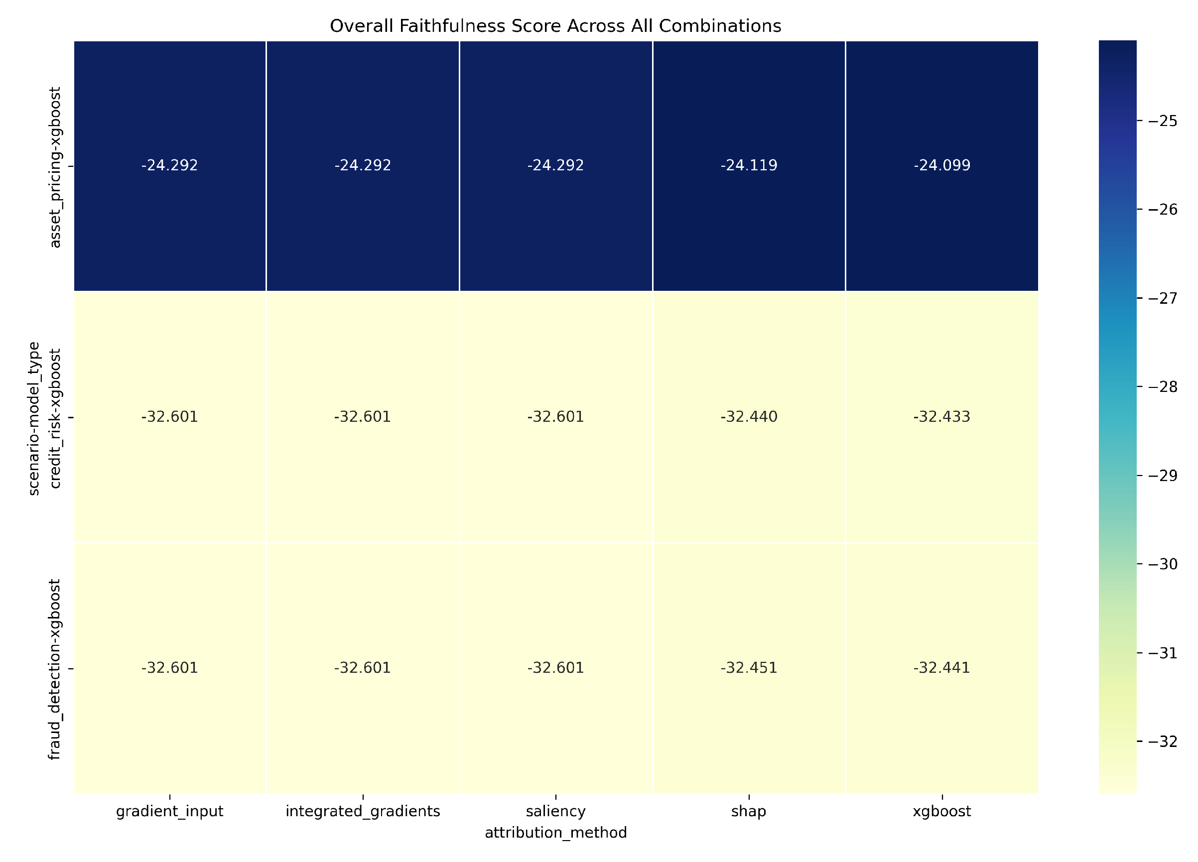
Figure 2.
Overall Faithfulness Score by Attribution Method and Scenario (for XGBoost Models).
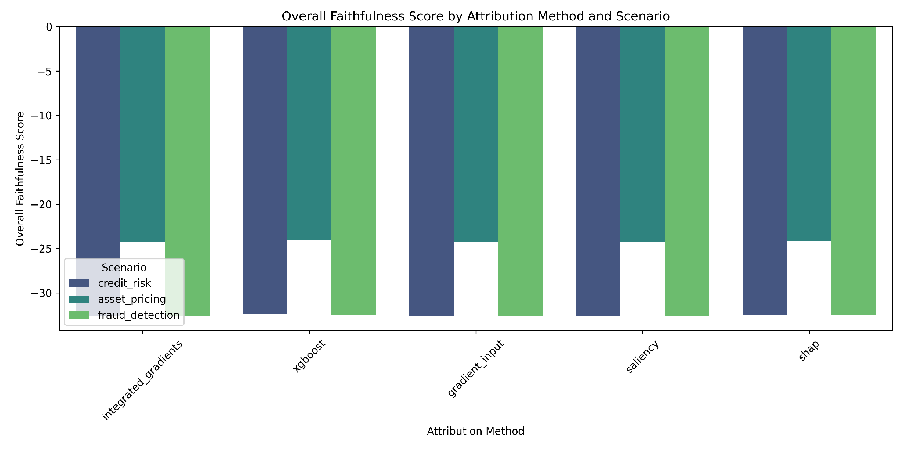
Figure 3.
Top-K Accuracy by Attribution Method and Scenario (for XGBoost Models).
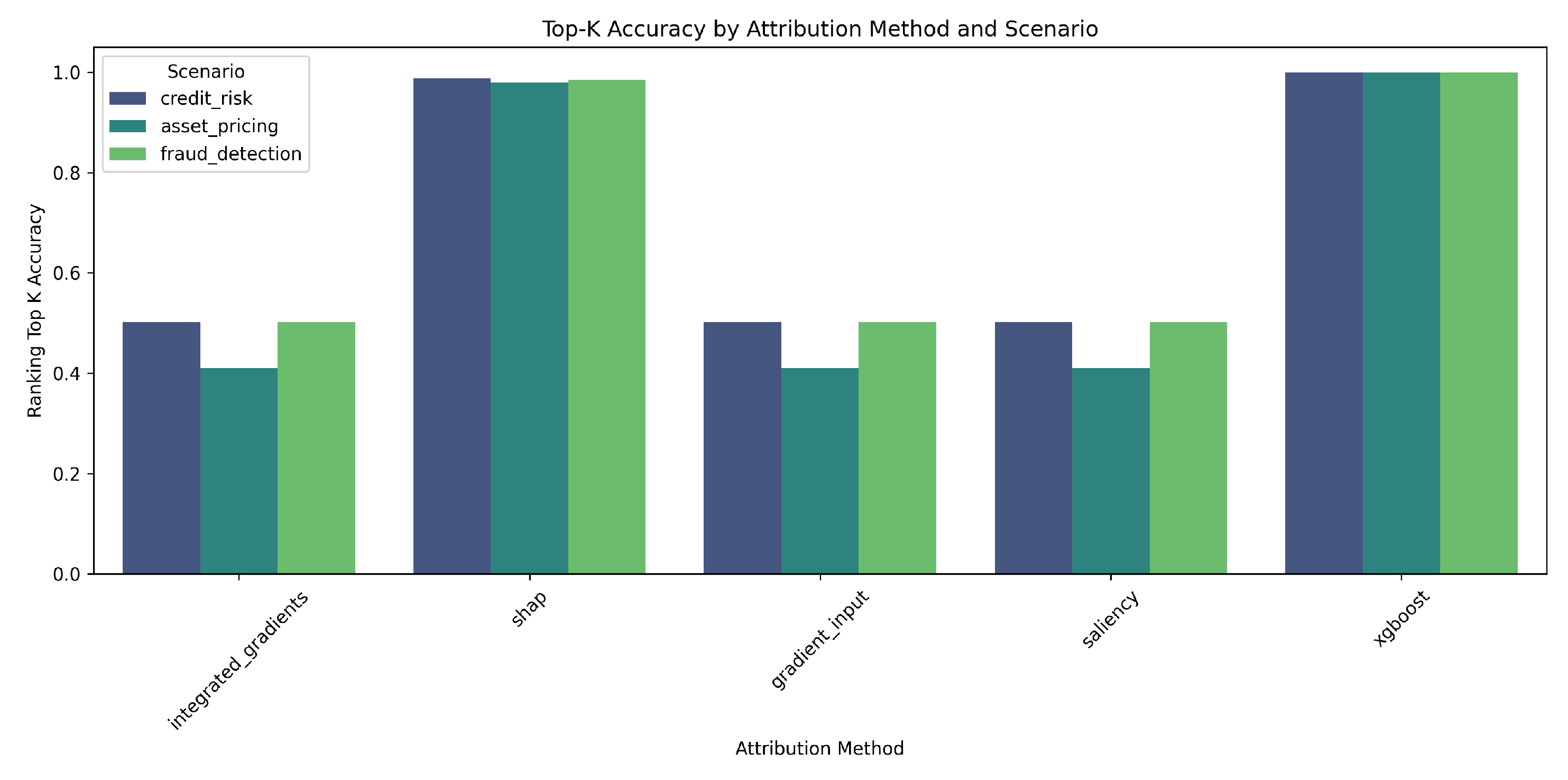
Figure 4.
Mean XGBoost Built-in Attribution Magnitude - XGBoost Model (Asset Pricing). Causal features (fundamental_) are blue; non-causal (spurious_) are red.
Figure 4.
Mean XGBoost Built-in Attribution Magnitude - XGBoost Model (Asset Pricing). Causal features (fundamental_) are blue; non-causal (spurious_) are red.
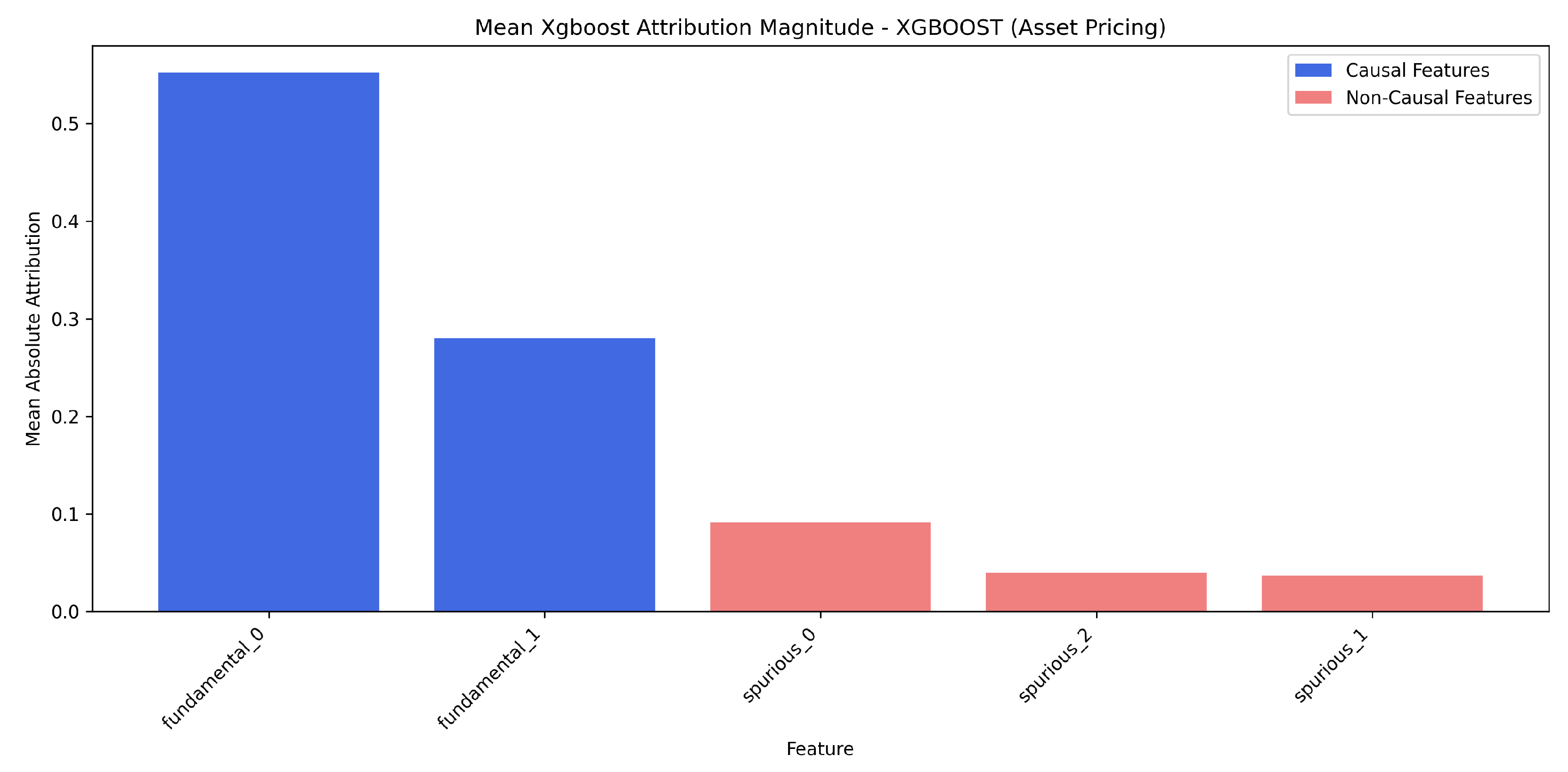
Figure 5.
SHAP Attributions for XGBoost Model (Asset Pricing).
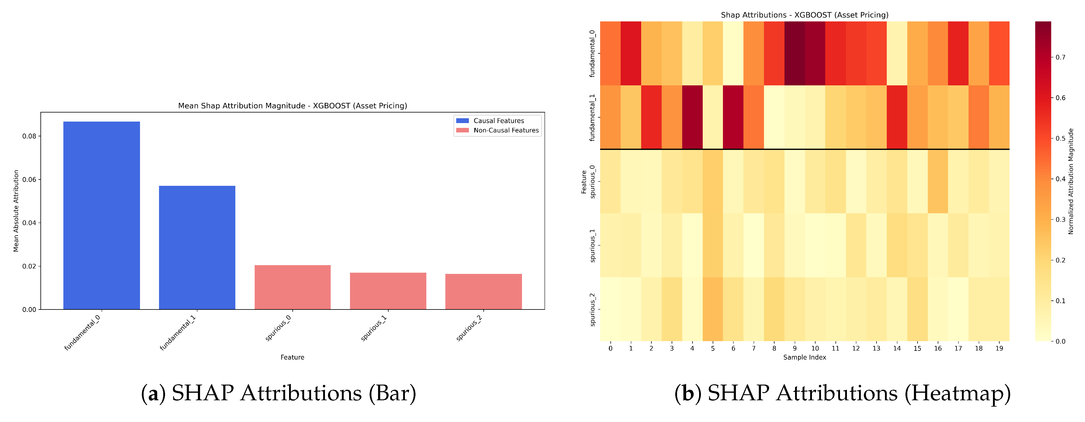
Figure 6.
Mean XGBoost Built-in Attribution Magnitude - XGBoost Model (Credit Risk). Causal features (behavioral_) are blue; non-causal (proxy_) are red.
Figure 6.
Mean XGBoost Built-in Attribution Magnitude - XGBoost Model (Credit Risk). Causal features (behavioral_) are blue; non-causal (proxy_) are red.
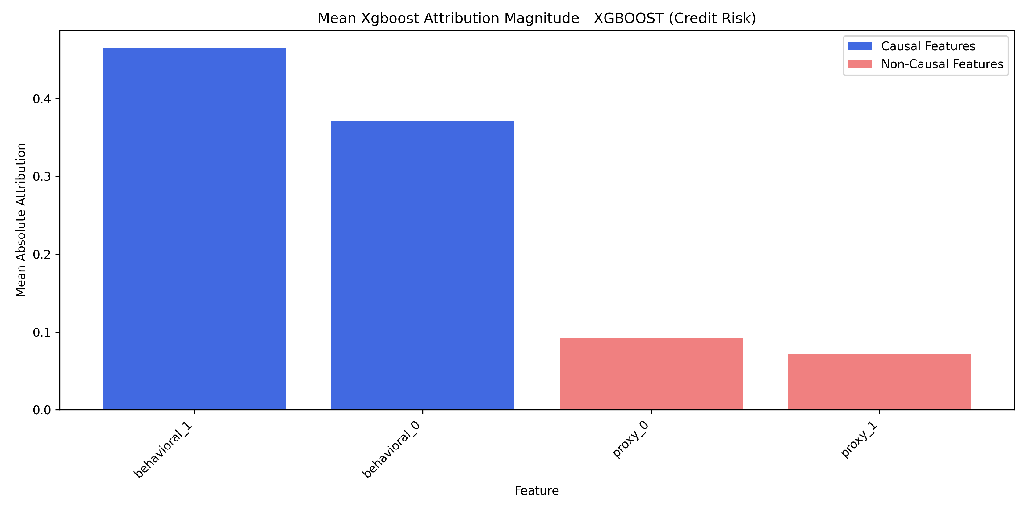
Figure 7.
SHAP Attributions for XGBoost Model (Credit Risk).

Figure 8.
Mean XGBoost Built-in Attribution Magnitude - XGBoost Model (Fraud Detection). Causal features (anomaly_) are blue; non-causal (indirect_) are red.
Figure 8.
Mean XGBoost Built-in Attribution Magnitude - XGBoost Model (Fraud Detection). Causal features (anomaly_) are blue; non-causal (indirect_) are red.
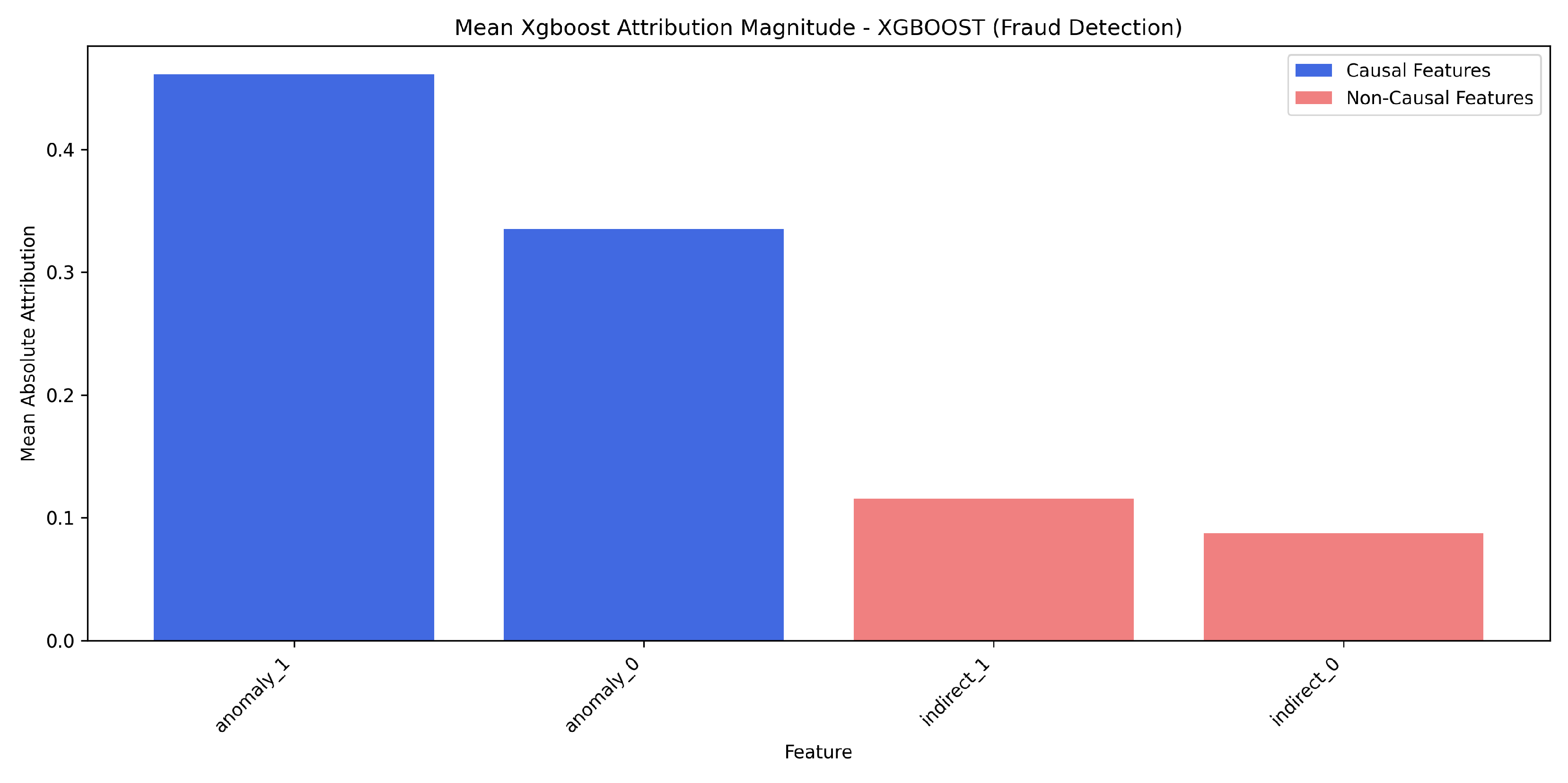
Figure 9.
SHAP Attributions for XGBoost Model (Fraud Detection).

Table 1.
Overall Model Performance. Data from model_performance.csv.
| Scenario | Model Type | Accuracy | F1 Score | MSE | R² |
| asset_pricing | mlp | N/A | N/A | 0.2362 | 0.9402 |
| asset_pricing | lstm | N/A | N/A | 1.5332 | 0.6116 |
| asset_pricing | xgboost | N/A | N/A | 0.1806 | 0.9543 |
| credit_risk | mlp | 0.9444 | 0.9448 | N/A | N/A |
| credit_risk | lstm | 0.8998 | 0.9005 | N/A | N/A |
| credit_risk | xgboost | 0.9650 | 0.9653 | N/A | N/A |
| fraud_detection | mlp | 0.9890 | 0.8898 | N/A | N/A |
| fraud_detection | lstm | 0.9821 | 0.8212 | N/A | N/A |
| fraud_detection | xgboost | 0.9957 | 0.9561 | N/A | N/A |
Table 2.
Summary of Attribution Method Performance (on XGBoost Models, Averaged Across Scenarios). Data from report.md / all_faithfulness_metrics.csv.
Table 2.
Summary of Attribution Method Performance (on XGBoost Models, Averaged Across Scenarios). Data from report.md / all_faithfulness_metrics.csv.
| Attribution Method | Overall Score | Top-K Accuracy | Attribution Ratio |
| xgboost | -29.6574 | 1.0000 | 5.4751 |
| shap | -29.6700 | 0.9837 | 3.8490 |
| saliency | -29.8310 | 0.4710 | 0.9961 |
| gradient_input | -29.8310 | 0.4710 | 0.9961 |
| integrated_gradients | -29.8310 | 0.4710 | 0.9961 |
Disclaimer/Publisher’s Note: The statements, opinions and data contained in all publications are solely those of the individual author(s) and contributor(s) and not of MDPI and/or the editor(s). MDPI and/or the editor(s) disclaim responsibility for any injury to people or property resulting from any ideas, methods, instructions or products referred to in the content. |
© 2025 by the authors. Licensee MDPI, Basel, Switzerland. This article is an open access article distributed under the terms and conditions of the Creative Commons Attribution (CC BY) license (http://creativecommons.org/licenses/by/4.0/).
Copyright: This open access article is published under a Creative Commons CC BY 4.0 license, which permit the free download, distribution, and reuse, provided that the author and preprint are cited in any reuse.


