
Submitted:
10 May 2025
Posted:
13 May 2025
You are already at the latest version
Abstract
The article presents a new method for evaluating investment projects in uncertain conditions, assuming that uncertainty may have been two origins: aleatory (related to randomness) and epistemic (due to incomplete knowledge). Epistemic uncertainty is rarely considered in investment analysis which can result in undervaluing the future opportunities and risks. Our approach utilizes the Datar-Mathews Method (DM Method) to gather relevant information regarding the potential value of real option. By combining probabilistic and possibilistic approaches, proposed valuation model incorporates hybrid Monte Carlo simulation and a random-fuzzy Geometric Brownian Motion, considering the interdependence between parameters. The result of the hybrid simulation is a pair of upper and lower cumulative probability distributions, known as a p-box, which represents the uncertainty range of the Net Present Value (NPV). We propose three transformations of the p-box into a subjective probability distribution, which allow decision-makers to incorporate their subjective beliefs and risk preferences when performing real option valuation. Thus, our approach allows the combination of objective available information about valuation of investment with the decision-maker's attitude in front of partial ignorance. To demonstrate the effectiveness of our approach in practical scenarios, we provide a numerical illustration that clearly showcases how our approach delivers a more precise valuation of real options.
Keywords:
Real options
; Datar-Mathews Method
; possibility theory
; investment decision
; hybrid Monte Carlo simulation
1. Introduction
The Datar-Mathews Method (DM Method) is a particularly interesting but still relatively underexplored area in simulation-based real option valuation (ROV). The method proposed by Datar and Mathews in 2004 provides an easy way to determine the real option value of a project by using the average of positive outcomes [1,2]. It uses Monte Carlo simulation to propagate uncertainty and to create payoff distribution of an investment alternative. The resulting payoff distribution is flexible, allowing for any compounding interval and free selection of discount rates [3]. Additionally, the results of the DM Method converge with the Black & Scholes result when the Monte Carlo simulation is run enough times. In this article, we propose a method for performing DM Method in a hybrid environment, which refers to a scenario where the parameters utilized for evaluating the investment cannot be precisely determined.
In real option valuation the accuracy of input parameters greatly influences the financial terms, such as cash flow and profit. Analysts frequently estimate parameters using past data and simultaneously make subjective guesses about future economic changes [4,5,6]. It results in the additional type of uncertainty in describing parameters, which, apart from random uncertainty, arises from a lack of knowledge or inherent vagueness [7]. The exclusive reliance on probability theory in these situations can result in a false sense of precision and an incorrect assumption that outcomes are inherently predictable and repeating in nature [8]. There is therefore a natural need to distinguish between different types of uncertainty in ROV.
Entrepreneurial activities encompass different levels of informational reliability, giving rise to situations where risks are linked to the probabilities of expected outcomes, while uncertainty arises when these probabilities cannot be precisely determined. It follows from the fact that valuing investment projects usually involves both types of uncertainty - aleatoric and epistemic. Aleatoric uncertainty is observed variability while epistemic uncertainty arises from incomplete knowledge. To effectively capture non-probabilistic uncertainty, it becomes crucial to incorporate to the model both probabilistic and possibilistic approaches [9]. Experts’ opinions or imprecise estimates may be introduced to the model in the form of possibilistic distribution as they better express vagueness, imprecision, or ambiguity [10]. In the field of ROV, the probabilistic Black-Scholes (B-S) model provides robust framework to model aleatoric uncertainty of many variables such as market size or product prices [5,6,11,12,13]. Therefore, a combination of both probabilistic and possibilistic approaches is necessary for accurately modelling and evaluating the uncertainties that exist in ROV.
Several factors led us to writing of this article. The first is that pure probabilistic approach is difficult to use in valuing investment projects using DM Method due to inherent vagueness that investors encounter. The second factor is the significant reliance on expert estimates in the metallurgical industry, where investment lifecycles typically span 10-12 years. Moreover, the relevance of historical data diminishes rapidly after 2-3 years, making it impractical to assert any predictive value of time series beyond 5 years [14]. The final reason is the interdependency among different products' demands. This connection creates a challenge when trying to forecast the demand for a single product in isolation, as it depends on the demand for other products within the same product line [15].
This study introduces a novel method for valuing investment projects that accounts for both imprecise and random uncertainties, while explicitly modeling the interdependencies among parameters within the Brownian Motion framework. Conventional ROV models tend to overlook the relationships between parameters, which can result in inaccurate forecasts and less precise valuation [4,7,15,16]. While some research has examined the correlation between parameters when using a probabilistic approach [5], current methods have limitations in fully addressing the complexities of aleatory and epistemic uncertainty. By incorporating these correlations in the DM, the proposed approach can provide a more realistic and precise evaluation of investment projects, while also accounting for the vagueness and randomness of the decision-making context.
The structure of the article is as follows: Firstly, we conducted a comprehensive review of real option in a hybrid environment. Next, we introduced the method of propagating uncertainty in such an environment using Monte Carlo simulation. Subsequently, we explored strategies for selecting subjective probability distributions that consider the decision-maker's perspective when faced with incomplete knowledge. To illustrate the effectiveness of our approach, we provided a clear example demonstrating how it enhances the precision of real options valuation.
2. Fuzzy Sets in Real Options Pricing
Fuzzy set theory has emerged as a prominent tool for addressing uncertainty in real option valuation, particularly when precise probabilistic data is unavailable. Many papers explore the possibility of using fuzzy sets or possibility theory to real options valuations. Carlsson et al. [17] developed a methodology for valuing options on R&D projects, in which future cash flows were estimated by trapezoidal fuzzy numbers. They presented a fuzzy mixed integer programming model for the R&D optimal portfolio selection problem. Carlsson and Fuller [8] use possibility theory to study fuzzy real option valuation. The present values of expected cash flows and expected costs are estimated by authors also by trapezoidal fuzzy numbers. They determined the optimal exercise time by the help of possibilistic mean value and variance of fuzzy numbers. Garcia [18] used the fuzzy real options valuation model in a real investment project from the energy sector. In Garcia's study, the theoretical framework proposed by Carlsson and Fullér [8] is applied to analyze the timing and selection of power plants from among various investment alternatives. Further, the study conducted by Allenotor and Thulasiram [19] employs a fuzzy trinomial real options model for the valuation of grid resources, substantiating the model's applicability through empirical analysis. Additionally, Tao [20] formulated an extensive methodology that integrates fuzzy risk assessment with a real options strategy, specifically for the evaluation of information technology investments in nuclear power stations. Zeng et al. [21] compared the application of traditional net present value method with real options in investment evaluations, analysed the uncertainty of power grid investment project, and discussed how to make the investment decision when investment cost and cash flow are both fuzzy numbers. Kahraman and Ucal [22] used the certainty equivalent approach for real options valuation in an oil investment with fuzzified data. Ho and Liao [23] propose a fuzzy approach for investment project valuation in uncertain environments from the aspect of real options. Lee et al. [12] utilized the principles of fuzzy decision theory combined with Bayes' theorem to assess fuzziness in option analysis practices.
However, it should be emphasized that none of the above-mentioned studies consider the problem defined in the first part of this article. In systematic review of the interactions between fuzzy set theory and option pricing conducted in [9], the fuzzy-random approach to option pricing was represented in approximately 35% of 240 reviewed papers. However, fuzzy real option was only represented by 13 papers. To the knowledge of the authors, there are few approaches to the analysis of real options in a hybrid environment. In [24] valuation of portfolio of real option under both type of uncertainty is presented. In [25] the generalised fuzzy-stochastic multi-mode real options model is developed. The [26] introduces a fuzzy-random extension of the Ho–Lee term structure model by incorporating fuzzy volatility into a binomial lattice framework, enhancing the pricing of interest rate derivatives like caplets under uncertainty.
The equivalent of the DM Method in a fuzzy environment is the "fuzzy pay-off" method proposed by Collan (a good summary can be found in [27]) (FROV). Collan in [28] compares the use of the Datar-Mathews method and the fuzzy pay-off method, in the analysis of investment cases with different levels of complexity. The results of the two methods are compared through numerical illustrations, showing that FROV is sufficient for problems with low complexity, but the DM Method is better suited for more complex ones. In [29] Borges states that there are situations in which the original “fuzzy pay-off” calculates the real option value to be negative, what is theoretically incorrect. He proposed the centre of gravity approach to real option valuation (PROBROV). Stoklasa in [30,31] presents possibilistic method for real ROV and compares aforementioned methods and fully possibilistic fuzzy ROV (POSROV).
Many prevailing theories in judgment and decision-making treat uncertainty as a singular concept. However, in our approach, we differentiate between two distinct types of uncertainty: epistemic (events that are potentially knowable) and aleatory (inherently random events). It's crucial to emphasize that, within our framework, this differentiation leans more towards a philosophical perspective rather than a purely pragmatic one. This approach gaining again popularity [32,33].
3. Materials And Methods
3.1. Modelling Uncertainty by Correlated Random-Fuzzy Geometric Brownian Motion (GBM)
The standard method for evaluating real options assumes that the value of the parameter will fluctuate according to a Geometric Brownian Motion (GBM) over a defined period. The parameter q follows GBM, if it satisfies the diffusion equation [4,34,35,36]:
where , and μ and σ are drift and volatility. Applying Ito’s Lemma and Euler discretization over interval , we can write the formulas for the prediction qt [4,34,35,36]
where Z is independent, normal random variate. Frequently, the available statistical data are inadequate or unsuitable for estimating parameters such as and . In scenarios where statistical data are insufficient, these parameters are estimated or refined by subject matter experts. Consequently, and become imprecise variables, aptly represented using fuzzy numbers. In our approach, when confronted with insufficient statistical data, we address the uncertainty in drift and volatility by representing them as possibilistic parameters: , described by fuzzy numbers. Consequently, Equation (2) can be rewritten as
where is random-fuzzy variable.
This method allows for the differentiation between uncertainties stemming from aleatory and epistemic sources to provide more realistic representation of GBM. It is noteworthy that when predicting the fluctuation of q, the literature typically assumes that all values in triple are represented by fuzzy numbers, resulting in a fuzzy variable as the outcome of the process. However, in our scenario, we encounter a combination of possibilistic and probabilistic .
To better understand what is meant by a possibilistic distribution, it is helpful to consider its roots in possibility theory. As described by Dubois and Prade [37], a possibility distribution—also known as a fuzzy number or a nested interval—represents an alternative to probability for encoding expert opinions. It maps intervals of parameter values to degrees of possibility (μ), which indicate how plausible each value is. These intervals, called α-cuts, provide bounds that reflect varying levels of confidence. For instance, the support of the distribution includes all possible values (μ = 0), while the core identifies the most plausible value (μ = 1). This allows a flexible and intuitive way to express epistemic uncertainty when precise probabilities are difficult to assign.
The versatility of Equation (3) causes that it can effectively represent various parameters such as unit prices, raw materials prices, or market volumes. These parameters are often correlated that deeply impact the final valuation outcome. Therefore, incorporating these interdependencies in the model is crucial for achieving precise and reliable results. To incorporate this correlation, we use the method describe in [38]. Let's suppose that we analyse I parameters. Additionally, it is assumed that there may be defined subsets of correlated parameters . Each Ik includes subset of correlated parameters. Therefore, Eq. (3) can be expressed as the following forecasting model for parameter qi
Here, it is assumed that and are possibilistic parameters, is correlated random normal variate and is random-fuzzy variable. To define , the Cholesky decomposition may be utilized to decompose the correlation matrix (as described in [39]).
Possibilistic distribution may be viewed as a nested set of intervals (called α-cut)
Interdependence between and , can be modelled by interval regression [40]. Below, we present the equations that define the relationships between these variables, using the notation of α-levels [38]
where , represent the coefficients of the interval regression equations, which are pivotal in establishing the dependencies between parameters and . These coefficients and can be ascertained using the method proposed by Hladik and Černy (crisp input-crisp output variant) [40,41].
3.2. Uncertainty Propagation
The uncertainty propagation is achieved through hybrid simulation, which combines the Monte Carlo technique with the extension principle of fuzzy set theory. The method has been applied across various fields, such as LCA [42], human health risk assessment [43], construction [44] or environmental science [45]. It’s based on assumptions of IRS (Independent Random Set) simulation proposed by Baudrit [46].
Let represents incremental cashflow of investment in year (T being the economic life-cycle of project). To perform hybrid simulation, all fuzzy variables are partitioned into into α-cuts with step .
Using the α-levels notation, the constraints on the possibilistic parameters and can be defined as follows:
Consequently, Eq. (8) and (9) constitute additional constraints in ICF calculation. The realization of is sampled from the probability distributions with Cholesky decomposition [47]. Formally, the hybrid simulation is presented in Algorithm 1. The prediction of future parameter values in the simulation loop is based on Equation (4), which captures the hybrid uncertainty propagation through random-fuzzy Geometric Brownian Motion with parameter interdependencies.
| Algorithm 1 Calculation of payoff distribution in hybrid environment |
|
Require: J, , T begin Set j=0 while while calculate sup() and inf() of (,,0) (Eq.4) subject to α-level constraints (Eq 8,9) interdependence between (Eq.6,7) for t = 0 to T-1 Generate vector of (MC Sampling with Cholesky decomposition) Forecast vector of (Eq. 4) Solve subject to financial constraints Solve subject to financial constraints Compute j = j + 1 end |
The output of hybrid simulation is set of random intervals . To obtain a payoff distribution from these results, the Dempster-Shafer theory is applied [48]. Let be a non-empty set called a Frame of Discernment, that describes all possible interval values of the NPV (Net Present Value) of the evaluated investment. The simulation results yield a collection of premises (called focal elements)
Let m be a function assigning a mass probability to each , such as , where A is the number of -levels used in the simulation. The belief regarding the occurrence of a given NPV value can be described by a pair of probabilities (belief):
and (plausibility)
This pair defines an interval commonly interpreted as the upper and lower probability bounds of .
Let be non-decreasing functions such as, . An interval
is called probability box (p-box), and functions i are called upper and lower cumulative payoff distribution. The exact form of the cumulative distribution function is unknown, but it is known to lie between these bounds. It can be shown [46] that if the , then . Thus, the set of premises can be transformed into a p-box representing the upper and lower bounds of the cumulative distribution for NPV outcomes.
The p-box can be interpreted in two ways: as bounds on the cumulative probability associated with a specific npv value, or as the tightest possible bounds on the distribution function given the available information. It is important to note that the p-boxes obtained from hybrid simulation are non-parametric—they are constructed without any assumptions about the shape of the underlying distribution of the variable of interest.
Ellsberg's experiments [49] show that choices in risky situations may differ from those in situations where information about chances are imprecise. Ellsberg introduced the concept of ambiguity, which is a state between complete ignorance and full knowledge of probability. Ambiguity arises from low information reliability or information inconsistencies [50]. Mathematically, ambiguity is reflected in situations where a decision maker deals with risk described using upper and lower distribution functions [51]. The decision maker aims to reduce ambiguity by finding a transformation that allows to convert the p-box into a subjective cumulative payoff distribution function . The construction of a subjective probability distribution is, in a sense, imposed on the decision-maker, who, upon encountering the ambiguity of simulation outcomes, is compelled to express their belief in the form of a probability distribution, even if his or her actual knowledge may not sufficiently justify the selection of one distribution over another.
3.3. Transformation of p-Box into Subjective Payoff Distribution
Different strategies can be applied to choose the subjective cumulative distribution function depending on the decision-maker's preferences and the decision context.
The pignistic transformation approach was proposed by Smets [52,53], is grounded in Laplace's principle of insufficient reason. It is identical to the so-called Shapley value used in cooperative game theory as a fairness principle for sharing benefits across members of coalitions. It treats each focal element from p-box result set as a set of payoffs with a unit mass probability . The expected value of each interval is derived by assuming a uniform distribution across the interval . The value of is calculated as [52]
This distribution reflects a neutral attitude, where the decision-maker "bets" equally on all possible outcomes within the specified intervals. It serves as the least biased representation of the decision maker's state of knowledge, aligning with the observed outcome of simulation [52]. In this transformation, the decision maker does not introduce any additional information into the model.
The Hurwicz criterion provides a way to interpolate between the best-case (upper bound) and worst-case (lower bound) scenarios represented by the p-box [54]. By using this criterion, Jeffrey introduced the concept of ambiguity, which represents a state between complete ignorance and perfect knowledge of probability. The ambiguity distribution may be defined as follows:
where takes values from 0 to 1 and is called the indicator of the pessimism (optimism) of a decision maker. Optimism index may be treated as a simple measure of belief in expert’s opinion.
The third approach is a generalization of the credibility theory proposed by Liu [55]. Dubois [54] extends the measure proposed by Liu with the coefficient of risk aversion β
For β=0.5, is equal to the Liu’s credibility distribution. Credibility distribution may be treated as decision maker attitude in the face of uncertainty. Polarization and vagueness represent systematic biases in decision-making when confronted with uncertainty. Polarization occurs when probabilities significantly deviate from the average, reflecting overconfidence, while vagueness involves adjusting probabilities closer to the average, often as an overcorrection to polarization or due to manipulation for favourable average outcomes. The Hurwitz criterion and Liu's Credibility distribution are complementary to each other, but they should be used in different scenarios. This approach is similar to those propose in [27,29,56].
The choice of strategy to transform the p-box into a cumulative distribution function depends on the analyst and scenario. Each of the strategies is valuable in different situations (which will be discussed in the case study). It is usually necessary to compare all strategies simultaneously.
After choosing a strategy, the cumulative distribution function is transformed into a probability density function j or payoff distribution This allows for the specification of a payoff distribution that enables the determination of the ROV.
3.4. Datar-Mathews Method in Random-Fuzzy Environment
In its classical form, the DM method relies on Monte Carlo simulation to model the uncertainty associated with investment project. The analysis begins by identifying the parameters that drive profitability and describing their uncertainty in terms of costs and revenues. A Monte Carlo run then generates the probability distribution of the project’s net present value (NPV). In the case of complex computational models, it may be necessary to implement parallel computing to speed up the Monte Carlo simulation [57]. The project is subsequently interpreted as a call option: negative NPVs are set to zero, reflecting the real-world practice of abandoning unprofitable ventures.
The ROV is calculated as
where Ur is probability that the investment will be profitable (success ratio) and denotes the expected value of the positive part of the NPV distribution. Figure 1 illustrates how the Datar–Mathews method can be applied in a hybrid (probabilistic–possibilistic) environment.
3.5. Comparison with Existing Approaches
Before we proceed to the analysis of the numerical case, we wanted to describe the similarities and differences between our approach and the fuzzy-pay off method for real option valuation (FROV) [27]. Both approaches are based on the Datar-Matthews method but differ in their assumptions. Although, both approaches have their roots in possibility theory [54], we employ a fuzzy-random approach, whereas FPOV utilizes pure fuzzy.
In both approaches, the value of real option is calculated by multiplying the “centroid” of the positive side of the NPV distribution by the proportion of the area of the NPV distribution that represents positive outcomes. The distinction lies in the fact that in our approach, we determine this value based on the subjective probability distribution of NPV derived from the p-box, while FROV utilizes fuzzy NPV for this purpose. Additionally, we use the expected value as the centroid, while variants of FPOV utilize possibilistic mean, center of gravity, or other interpretations. In essence, we have control over the shape of the NPV distribution, whereas FPOV interprets its expected value based on the distribution.
It should be emphasized that using the method proposed by us, ROV is possible with both methods - ours and Collan's. This is made possible by relying on hybrid simulation, which yields a p-box. It can be demonstrated that this structure can be transformed into both a probability distribution and a fuzzy random variable, thereby resulting in a fuzzy NPV [58,59]. Further research is needed to determine the relationship between our approach and the approach proposed in Collan's work.
4. Results
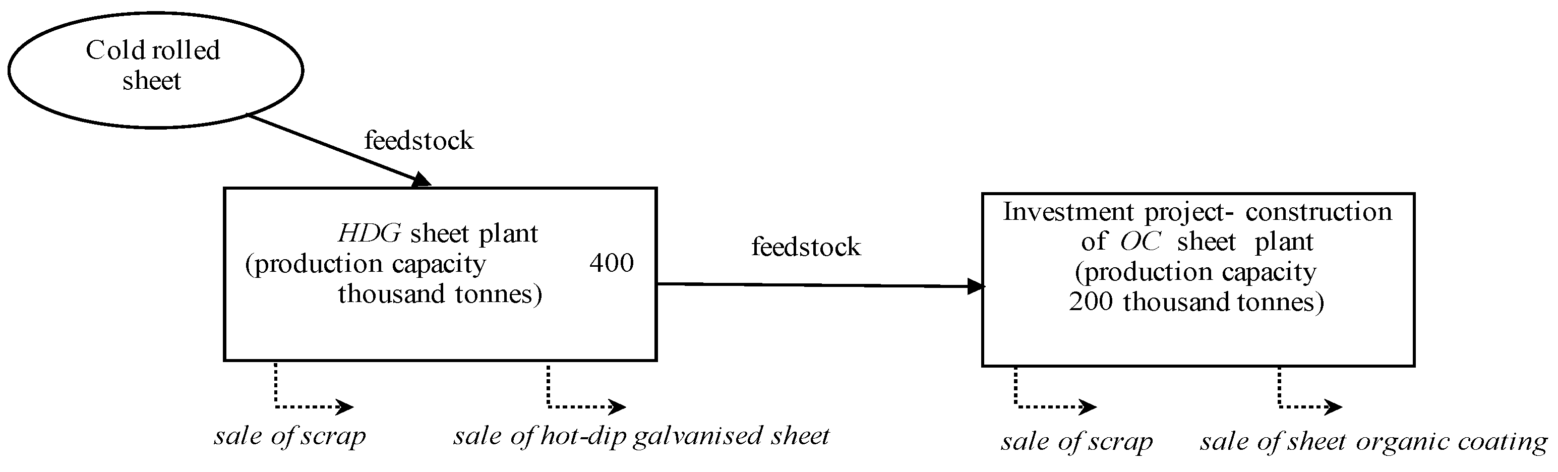
This example considers a steel manufacturer that is weighing the construction of a new production line for organic-coated sheets. The firm currently produces conventional sheets but now has an opportunity to adopt organic-coating technology. Management must determine whether building the new facility is economically justified. Before construction can begin, the company must prepare project documentation and complete environmental assessments to obtain the required permits; we assume these preparatory activities will cost USD 20,000.
To assist in the decision-making process, the company conducts net present value (NPV) and real option analyses. These analyses involve assessing the future cash flows with the help of experts. The key question is whether the company should invest the funds to obtain a return on investment.
Model for Estimating the Value of Project in Hybrid Environment
In this section we introduce the NPV model that underpins the real-option valuation of a hypothetical production system (see Fig. 2). The model extends the framework described in [58].
The project under consideration is the construction of a new plant for manufacturing organic-coated (OC) steel sheet. OC sheet is produced from hot-dip-galvanised (HDG) sheet and enjoys both a broader range of applications and a higher unit value. The main input to the process is cold-rolled (CR) sheet, which is first converted to HDG sheet; part of that output is sold directly, while the rest is further processed into OC sheet and sold. Both the HDG and OC stages generate steel-scrap by-products that are likewise sold.
Figure 2.
Description of the analysed production setup.
To apply the Datar–Mathews (DM) method we must derive φ (npv), the NPV density obtained from a Monte-Carlo simulation of the new OC plant. This calls for incremental cash-flow modelling: cash flows in the investment scenario (which includes the OC facility) are compared with those in the baseline scenario (status quo without the new plant). The project NPV can then be computed with Equations (18)–(32).
The notation used in model are presented in Table 1.
The net present value of the proposed OC-sheet line is obtained with Eq. (18), in which the incremental cash-flows are defined by Eq. (19) and decomposed by Eqs. (20)–(29) into operating profit after tax, depreciation, variable input costs and fixed overheads. The annual variation in net working capital is captured by Eq. (30), while the stock of working capital itself is evaluated with the revised Eq. (31), which relates cash, inventories, receivables and payables to four turnover ratios (CTR, ITO, DTR and DTP). At the end of the planning horizon the model releases tied-up capital according to the Wilcox convention [47] implemented in the revised Eq. (32), i.e. it recovers 100% of cash, 70% of the book value of inventories and receivables, and the full 100% of outstanding payables
Prices and apparent consumption for the analyzed products are inter-related rather than independent, displaying complex patterns of correlation and mutual dependence. Two relationship types can be distinguished: correlations and reciprocal dependencies. The pair-wise price correlations are summarized in Table 2, and the correlation coefficient between the apparent consumption of HDG sheet and OC sheet is 0.532.
Interval-regression coefficients that characterize the interdependencies among the drift parameters (μᵢ) of the individual price series are provided in Table 3; the corresponding coefficients for apparent consumption appear in Table 4.
For a steel plant operating with the leverage typical of the industry, we assume a real weighted-average cost of capital (WACC) of 10% p.a. and a real risk-free rate of 5% p.a. [4].
Historical data for 1996–2022 show that, in real terms, OC-sheet prices increased at an average annual rate of 0.89%. Over the same period, average annual growth rates were 1.46% for HDG sheet, 1.73% for CR sheet, and 1.63% for scrap. To generalize these trends we represent the common drift term across all products by the trapezoidal fuzzy number (0.85%, 1.10%, 1.30%, 1.50%), reflecting the structural shifts observed in the market—particularly during the 2006–2007 economic boom.
A review of apparent-consumption data for 1996 – 2022 shows that demand for HDG sheet and OC sheet grew on average by 7.55% and 8.65% per year, respectively. To generalise these dynamics, we adopt a common drift term for all products, expressed as the trapezoidal fuzzy number (6.0%, 6.5%, 7.0%, 7.5%), which captures the structural changes the sector underwent—particularly in the boom years of 2006 – 2007.
Volatility is estimated as the standard deviation of log-returns over 2000 – 2022. For prices the resulting annual volatilities are 15.02% (scrap), 19.04% (CR sheet), 18.67% (HDG sheet) and 12.86% (OC sheet); for apparent consumption they are 10.43% for HDG sheet and 15.03% for OC sheet. Consistent with the treatment of drift, we represent each volatility by a trapezoidal fuzzy number:
- Prices
- Scrap: (13.0%, 14.0%, 15.0%, 16.0%)
- CR sheet and HDG sheet: (15.0%, 17.0%, 18.0%, 20.0%)
- OC sheet: (10.0%, 11.0%, 12.0%, 13.0%)
- Apparent consumption
- HDG sheet: (8.0%, 9.0%, 10.0%, 11.0%)
- OC sheet: (12.0%, 13.0%, 14.0%, 15.0%)
Other cost assumptions are as follows. Variable production costs (energy, labour, maintenance) amount to roughly 116 USD per ton for HDG sheet and 182 USD per ton for OC sheet. Fixed operating costs are estimated at 31.28 million USD per year for the existing HDG line and an incremental 13.44 million USD per year for the proposed OC line. The OC-line capital outlay is about 42 million USD. Market-share targets are 30% for HDG sheet and 25% for OC sheet, reflecting their expected competitive positions.
Under these assumptions, the NPV of building OC-sheet plant was built. Figure 3 reports the resulting probability box, , for two cases: (a) when interdependencies among input parameters are included and (b) when they are ignored. P-boxes let us disentangle the effects of the two main kinds of uncertainty. Relaxing the dependency assumptions (case b) widens the gap between the lower and upper cumulative curves, signalling greater epistemic uncertainty. The vertical distance between these curves therefore measures epistemic uncertainty, whereas the shape of each curve captures the aleatory—or purely random—component. Recognising the difference helps decision-makers see whether risk stems mainly from limited knowledge and expert-judgement bias (epistemic) or from intrinsic variability in historical data (aleatory).
5. Discussion
Figure 3 shows the simulation results in the form of a p-box, accompanied by three cumulative distributions payoffs: pignistic, ambiguity (λ=0.5), and credibility (β=0.5). The corresponding results represented as a density function can be seen in Figure 4 and cumulative distribution function in Figure 5. Utilizing these transformations, the option's value was calculated using Eq (16). The NPV and ROV values can be found in Table 5.
The results presented in Table 5 provide a comprehensive comparison of the various approaches considered. Utilizing the data from Table 5 allows for conducting valuation analyses using both the Net Present Value (NPV) and Real Option Valuation (ROV) methods. The classical NPV analysis, irrespective of the transformation employed, indicates a negative decision regarding the initiation of the investment. Essentially, initiating a project that does not add value to the company would not be rational. Although the standard deviation remains consistent across scenarios, the substantial percentage difference between the optimistic and pessimistic probability bounds highlights the critical importance of considering the option value in investment decisions.
Conversely, adopting a real option analysis perspective provides an alternative viewpoint. Real option valuation offers insights into the project's potential upside value. If the potential benefits from the project exceed the cost of obtaining the real option, which enables capturing upside potential in response to changes, then acquiring the option becomes a sensible investment. In this analysis, three distinct outcomes are derived due to the application of three different ROV methodologies.
Using pure results from the hybrid simulation, the probability of success exhibits a broad range from 8% to 80%, and the corresponding ROV spans from 2 to over 26 thousands USD. The considerable disparity between the optimistic and pessimistic bounds emphasizes the importance of distinguishing between data accuracy and expert estimations in the valuation process. Decision-makers must evaluate whether to rely on this information for investment decisions. If they find the range excessively broad, they may opt for additional research to reduce subjective uncertainty represented by fuzzy numbers for GBM parameters. However, further analysis may not always be feasible due to various constraints. In such instances, decision-makers might opt for one of the available transformations.
The pignistic probability transformation can serve as a baseline reference. The unit mass probability represents the subjective probability for each interval . Here, "subjective" implies that is proportional to its appearance in simulation outcomes. This interpretation suggests the probability of epistemic states represented by . When each state within intervals is equally probable, the pignistic transformation aligns closely with pure Monte Carlo simulation. In our example, closely mirrors (with a success probability of 15%). Thus, the probability of success is influenced by the decision-maker's stance toward uncertainty and expert assessments.
The selection of other transformations depends on the perceived nature of epistemic uncertainty. The ambiguity transformation, as illustrated in this study using a weighting of 0.5, is particularly suitable for sensitivity analyses. This measure reflects the decision-maker’s confidence level in expert opinions, influencing the weighting of optimistic versus pessimistic probability bounds.
Finally, the third transformation reflects the decision-maker’s attitude towards uncertainty, indicating their preference for optimism or pessimism. This approach resembles the possibilistic fuzzy pay-off method for real option valuation described in [56]. It should be emphasized, however, that this transformation does not take into account investors' risk aversion. This transformation represents the investor's mental attitude towards the success of the investment or his epistemic knowledge about the effects of the investment.
Based on the pignistic transformation, the real option’s value is lower than the acquisition cost, implying a negative investment decision. However, when the ROVamb and ROVcred transformations are considered, the real option value exceeds the acquisition cost. Therefore, these transformations support the initiation of preparatory steps for building the organic coating plant, as this would create an opportunity to capitalize on future investments in the production of the replacement product.
6. Conclusions
This study introduces a novel hybrid approach to real option valuation that integrates probabilistic and possibilistic frameworks within the Datar-Mathews Method (DMM). To the best of our knowledge, this is the first adaptation of the DMM to explicitly accommodate both aleatory and epistemic uncertainties throughout the entire valuation process. By combining random and fuzzy representations of uncertainty, the proposed method provides a more comprehensive and realistic assessment of investment projects operating under deep uncertainty and limited data availability.
One of the key strengths of the presented hybrid DMM approach lies in its ability to differentiate between uncertainty arising from inherent randomness (aleatory) and that caused by incomplete knowledge (epistemic). This distinction enables decision-makers not only to model variability in market conditions and input parameters more accurately but also to explicitly recognize the role of subjective expert judgment in scenarios where historical data are scarce or unreliable. By avoiding the premature aggregation of these two types of uncertainty during simulation, the method allows for a transparent and traceable propagation of uncertainty throughout the valuation process.
In contrast to traditional real option valuation models, which often rely solely on probabilistic assumptions, the hybrid DMM introduces an additional analytical layer that reflects the decision-maker’s attitude toward uncertainty. Through the application of three different strategies for transforming p-box results into subjective probability distributions—pignistic, ambiguity-based, and credibility-based transformations—the method provides flexibility in capturing diverse decision-maker preferences, including optimism, pessimism, and varying degrees of confidence in expert assessments. This feature empowers practitioners to adjust the valuation according to their individual risk tolerance, epistemic beliefs, and strategic posture.
One of the key advantages of this hybrid DMM is its ability to effectively separate aleatoric and epistemic uncertainties in the decision-making process. As research shows [32], understanding the nature of uncertainty can help in designing interventions to improve judgment accuracy. Investors who see market uncertainty as stemming from a lack of knowledge or skill tend to seek expert guidance and react swiftly to new information, while those who view market uncertainty as driven by random processes are more inclined to diversify their portfolios to mitigate risk [33]. Unlike other methods, such as Fuzzy Real Options Valuation (FROV), this approach avoids aggregating these uncertainties during propagation through simulation. Additionally, it introduces an additional layer that explicitly requires decision-makers to address simulation results by considering potential issues like experts' over-optimism, reliance on heuristics, or other cognitive biases. Consequently, the proposed approach allows decision-makers to assess the influence of such factors on the final decision, while also providing quantitative descriptions of their approach to uncertainty.
Overall, this paper introduces a comprehensive and robust hybrid DMM that accounts for various sources of uncertainty and provides valuable insights for decision-makers grappling with real options under high uncertainty. By incorporating both aleatoric and epistemic uncertainties, the method enables a thorough analysis of investment projects and facilitates the integration of expert knowledge, ultimately bridging the gap between real-world decision-making and real option valuation.
Author Contributions
Conceptualization, B.G. and B.R.; methodology, B.G and B.R.; software, B.G.; validation, B.G. and A.P.; formal analysis, B.G. and A.P.; writing—original draft preparation, B.G.; writing—review and editing, A.P. All authors have read and agreed to the published version of the manuscript.
Funding
The APC was funded under subvention funds for the Faculty of Management and by- program “Excellence Initiative—Research University” for the AGH University of Krakow.
Institutional Review Board Statement
Not applicable.
Informed Consent Statement
Not applicable.
Data Availability Statement
The original contributions presented in this study are included in the article.
Conflicts of Interest
The authors declare no conflicts of interest.
References
- Datar, V.T.; Mathews, S.H. European Real Options: An Intuitive Algorithm for the Black-Scholes Formula 2005.
- Mathews, S.; Datar, V.; Johnson, B. A Practical Method for Valuing Real Options: The Boeing Approach. Journal of Applied Corporate Finance 2007, 19, 95–104. [Google Scholar] [CrossRef]
- Collan, M. Thoughts about Selected Models for the Valuation of Real Options. Acta Universitatis Palackianae Olomucensis. Facultas Rerum Naturalium. Mathematica 2011, 50, 5–12. [Google Scholar]
- Ozorio, L. de M.; Bastian-Pinto, C. de L.; Baidya, T.K.N.; Brandão, L.E.T. Investment Decision in Integrated Steel Plants under Uncertainty. International Review of Financial Analysis 2013, 27, 55–64. [Google Scholar] [CrossRef]
- Rębiasz, B.; Gaweł, B.; Skalna, I. Valuing Managerial Flexibility: An Application of Real-Option Theory to Steel Industry Investments. Operations Research and Decisions 2017, 27, 91–111. [Google Scholar] [CrossRef]
- Wu, H.-C. Using Fuzzy Sets Theory and Black–Scholes Formula to Generate Pricing Boundaries of European Options. Applied Mathematics and Computation 2007, 185, 136–146. [Google Scholar] [CrossRef]
- Zmeškal, Z. Generalised Soft Binomial American Real Option Pricing Model (Fuzzy–Stochastic Approach). European Journal of Operational Research 2010, 207, 1096–1103. [Google Scholar] [CrossRef]
- Carlsson, C.; Fullér, R. A Fuzzy Approach to Real Option Valuation. Fuzzy Sets and Systems 2003, 139, 297–312. [Google Scholar] [CrossRef]
- de Andrés-Sánchez, J. A Systematic Review of the Interactions of Fuzzy Set Theory and Option Pricing. Expert Systems with Applications 2023, 223, 119868. [Google Scholar] [CrossRef]
- Guerra, M.L.; Magni, C.A.; Stefanini, L. Value Creation and Investment Projects: An Application of Fuzzy Sensitivity Analysis To Project Financing Transactions 2022.
- Wu, H.-C. Pricing European Options Based on the Fuzzy Pattern of Black–Scholes Formula. Computers & Operations Research 2004, 31, 1069–1081. [Google Scholar] [CrossRef]
- Lee, C.-F.; Tzeng, G.-H.; Wang, S.-Y. A New Application of Fuzzy Set Theory to the Black–Scholes Option Pricing Model. Expert Systems with Applications 2005, 29, 330–342. [Google Scholar] [CrossRef]
- Gaweł, B.; Paliński, A. Long-Term Natural Gas Consumption Forecasting Based on Analog Method and Fuzzy Decision Tree. Energies 2021, 14, 4905. [Google Scholar] [CrossRef]
- Collan, M.; Fuller, R.; Mezei, J. A Fuzzy Pay-Off Method for Real Option Valuation. In Proceedings of the 2009 International Conference on Business Intelligence and Financial Engineering; July 2009; pp. 165–169. [Google Scholar]
- Huang, M.-G. Real Options Approach-Based Demand Forecasting Method for a Range of Products with Highly Volatile and Correlated Demand. European Journal of Operational Research 2009, 198, 867–877. [Google Scholar] [CrossRef]
- Xu, W.; Wu, C.; Xu, W.; Li, H. A Jump-Diffusion Model for Option Pricing under Fuzzy Environments. Insurance: Mathematics and Economics 2009, 44, 337–344. [Google Scholar] [CrossRef]
- Carlsson, C.; Fullér, R.; Heikkilä, M.; Majlender, P. A Fuzzy Approach to R&D Project Portfolio Selection. International Journal of Approximate Reasoning 2007, 44, 93–105. [Google Scholar] [CrossRef]
- Augusto Alcaraz Garcia, F. Fuzzy Real Option Valuation in a Power Station Reengineering Project. In Proceedings of the Proceedings World Automation Congress 2004, June 2004; 17, pp. 281–288. [Google Scholar]
- Allenotor, D.; Thulasiram, R.K. A Grid Resources Valuation Model Using Fuzzy Real Option. In Proceedings of the Parallel and Distributed Processing and Applications; Stojmenovic, I., Thulasiram, R.K., Yang, L.T., Jia, W., Guo, M., de Mello, R.F., Eds.; Springer: Berlin, Heidelberg, 2007; pp. 622–632. [Google Scholar]
- Tao, C.; Jinlong, Z.; Shan, L.; Benhai, Y. Fuzzy Real Option Analysis for IT Investment in Nuclear Power Station. In Proceedings of the Computational Science – ICCS 2007; Shi, Y., van Albada, G.D., Dongarra, J., Sloot, P.M.A., Eds.; Springer: Berlin, Heidelberg, 2007; pp. 953–959. [Google Scholar]
- Zeng, M.; Wang, H.; Zhang, T.; Li, B.; Huang, S. Research and Application of Power Network Investment Decision-Making Model Based on Fuzzy Real Options. In Proceedings of the 2007 International Conference on Service Systems and Service Management; June 2007; pp. 1–5. [Google Scholar]
- Uçal, İ.; Kahraman, C. Fuzzy Real Options Valuation for Oil Investments. Ukio Technologinis ir Ekonominis Vystymas 2009, 15, 646–669. [Google Scholar] [CrossRef]
- Ho, S.-H.; Liao, S.-H. A Fuzzy Real Option Approach for Investment Project Valuation. Expert Systems with Applications 2011, 38, 15296–15302. [Google Scholar] [CrossRef]
- Zmeškal, Z.; Dluhošová, D.; Gurný, P.; Kresta, A. Generalised Soft Multi-Mode Real Options Model (Fuzzy-Stochastic Approach). Expert Systems with Applications 2022, 192, 116388. [Google Scholar] [CrossRef]
- Maier, S.; Pflug, G.C.; Polak, J.W. Valuing Portfolios of Interdependent Real Options under Exogenous and Endogenous Uncertainties. European Journal of Operational Research 2020, 285, 133–147. [Google Scholar] [CrossRef]
- Andrés-Sánchez, J. de A Systematic Overview of Fuzzy-Random Option Pricing in Discrete Time and Fuzzy-Random Binomial Extension Sensitive Interest Rate Pricing. Axioms 2025, 14, 52. [Google Scholar] [CrossRef]
- Collan, M.; Fuller, R.; Mezei, J. A Fuzzy Pay-Off Method for Real Option Valuation. In Proceedings of the 2009 International Conference on Business Intelligence and Financial Engineering; July 2009; pp. 165–169. [Google Scholar]
- Kozlova, M.; Collan, M.; Luukka, P. Comparison of the Datar-Mathews Method and the Fuzzy Pay-Off Method through Numerical Results. Advances in Decision Sciences 2016, 2016, 1–7. [Google Scholar] [CrossRef]
- Borges, R.E.P.; Dias, M.A.G.; Dória Neto, A.D.; Meier, A. Fuzzy Pay-off Method for Real Options: The Center of Gravity Approach with Application in Oilfield Abandonment. Fuzzy Sets and Systems 2018, 353, 111–123. [Google Scholar] [CrossRef]
- Stoklasa, J.; Collan, M.; Luukka, P. Practical Possibilistic Fuzzy Pay-off Method for Real Option Valuation. Fuzzy Sets and Systems 2024, 492, 109072. [Google Scholar] [CrossRef]
- Stoklasa, J.; Luukka, P.; Collan, M. Possibilistic Fuzzy Pay-off Method for Real Option Valuation with Application to Research and Development Investment Analysis. Fuzzy Sets and Systems 2021, 409, 153–169. [Google Scholar] [CrossRef]
- Tannenbaum, D.; Fox, C.R.; Ülkümen, G. Judgment Extremity and Accuracy Under Epistemic vs. Aleatory Uncertainty. Management Science 2017, 63, 497–518. [Google Scholar] [CrossRef]
- Walters, D.J.; Ülkümen, G.; Tannenbaum, D.; Erner, C.; Fox, C.R. Investor Behavior Under Epistemic vs. Aleatory Uncertainty. Management Science 2023, 69, 2761–2777. [Google Scholar] [CrossRef]
- Wattanarat, V.; Phimphavong, P.; Matsumaru, M. Demand and Price Forecasting Models for Strategic and Planning Decisions in a Supply Chain. 2009.
- Bastian-Pinto, C.; Brandão, L.; Hahn, W.J. Flexibility as a Source of Value in the Production of Alternative Fuels: The Ethanol Case. Energy Economics 2009, 31, 411–422. [Google Scholar] [CrossRef]
- Marathe, R.R.; Ryan, S.M. On The Validity of The Geometric Brownian Motion Assumption. The Engineering Economist 2005, 50, 159–192. [Google Scholar] [CrossRef]
- Dubois, D.; Prade, H. Practical Methods for Constructing Possibility Distributions. International Journal of Intelligent Systems 2016, 31, 215–239. [Google Scholar] [CrossRef]
- Rebiasz, B. New Methods of Probabilistic and Possibilistic Interactive Data Processing. Journal of Intelligent & Fuzzy Systems 2016, 30, 2639–2656. [Google Scholar]
- Yang, I.-T. Simulation-Based Estimation for Correlated Cost Elements. International Journal of Project Management 2005, 23, 275–282. [Google Scholar] [CrossRef]
- Hladík, M.; Černý, M. Interval Regression by Tolerance Analysis Approach. Fuzzy Sets and Systems 2012, 193, 85–107. [Google Scholar] [CrossRef]
- Skalna, I.; Rebiasz, B.; Gawel, B.; Basiura, B.; Duda, J.; Opila, J.; Pelech-Pilichowski, T. Advances in Fuzzy Decision Making. Studies in Fuzziness and Soft Computing 2015, 333. [Google Scholar]
- Clavreul, J.; Guyonnet, D.; Tonini, D.; Christensen, T.H. Stochastic and Epistemic Uncertainty Propagation in LCA. Int J Life Cycle Assess 2013, 18, 1393–1403. [Google Scholar] [CrossRef]
- Guyonnet, D.; Coftier, A.; Bataillard, P.; Destercke, S. Risk-Based Imprecise Post-Remediation Soil Quality Objectives. Science of The Total Environment 2024, 923, 171445. [Google Scholar] [CrossRef]
- Islam, M.S.; Nepal, M.P.; Skitmore, M.; Attarzadeh, M. Current Research Trends and Application Areas of Fuzzy and Hybrid Methods to the Risk Assessment of Construction Projects. Advanced Engineering Informatics 2017, 33, 112–131. [Google Scholar] [CrossRef]
- Guyonnet, D.; Coftier, A.; Bataillard, P.; Destercke, S. Risk-Based Imprecise Post-Remediation Soil Quality Objectives. Science of The Total Environment 2024, 923, 171445. [Google Scholar] [CrossRef]
- Baudrit, C.; Dubois, D.; Guyonnet, D. Joint Propagation and Exploitation of Probabilistic and Possibilistic Information in Risk Assessment. IEEE Transactions on Fuzzy Systems 2006, 14, 593–608. [Google Scholar] [CrossRef]
- Rȩbiasz, B.; Gaweł, B.; Skalna, I. Hybrid Framework for Investment Project Portfolio Selection. In Advances in Business ICT: New Ideas from Ongoing Research; Pełech-Pilichowski, T., Mach-Król, M., Olszak, C.M., Eds.; Studies in Computational Intelligence; Springer International Publishing: Cham, 2017; pp. 87–104. ISBN 978-3-319-47208-9. [Google Scholar]
- Gaweł, B.; Rębiasz, B.; Skalna, I. Teoria Prawdopodobieństwa i Teoria Możliwości w Podejmowaniu Decyzji Inwestycyjnych. Studia Ekonomiczne 2015, 62–79. [Google Scholar]
- Wakker, P.P. Prospect Theory: For Risk and Ambiguity; Cambridge University Press, 2010; ISBN 978-1-139-48910-2. [Google Scholar]
- Schröder, D. Real Options, Ambiguity, and Dynamic Consistency — A Technical Note. International Journal of Production Economics 2020, 229, 107772. [Google Scholar] [CrossRef]
- Dubois, D.; Prade, H. Possibility Theory and Its Applications: Where Do We Stand. In Springer Handbook of Computational Intelligence; Kacprzyk, J., Pedrycz, W., Eds.; Springer Handbooks; Springer: Berlin, Heidelberg, 2015; pp. 31–60. ISBN 978-3-662-43505-2. [Google Scholar]
- Dubois, D.; Prade, H.; Smets, P. A Definition of Subjective Possibility. International Journal of Approximate Reasoning 2008, 48, 352–364. [Google Scholar] [CrossRef]
- Smets, P. Decision Making in the TBM: The Necessity of the Pignistic Transformation. International Journal of Approximate Reasoning 2005, 38, 133–147. [Google Scholar] [CrossRef]
- Dubois, D.; Guyonnet, D. Risk-Informed Decision-Making in the Presence of Epistemic Uncertainty. International Journal of General Systems 2011, 40, 145–167. [Google Scholar] [CrossRef]
- Liu, B. Uncertainty Theory. In Uncertainty Theory. In Uncertainty Theory: A Branch of Mathematics for Modeling Human Uncertainty; Liu, B., Ed.; Studies in Computational Intelligence; Springer: Berlin, Heidelberg, 2010; pp. 1–79. ISBN 978-3-642-13959-8. [Google Scholar]
- Stoklasa, J.; Luukka, P.; Collan, M. Possibilistic Fuzzy Pay-off Method for Real Option Valuation with Application to Research and Development Investment Analysis. Fuzzy Sets and Systems 2021, 409, 153–169. [Google Scholar] [CrossRef]
- Yang, X.; Li, C.; Li, X.; Lu, Z. A Parallel Monte Carlo Algorithm for the Life Cycle Asset Allocation Problem. Applied Sciences 2024, 14, 10372. [Google Scholar] [CrossRef]
- Ferson, S.; Kreinovick, V.; Ginzburg, L.; Sentz, F. Constructing Probability Boxes and Dempster-Shafer Structures; 2003; pp. SAND2002-4015, 809606. [Google Scholar]
- Dubois, D.; Prade, H. A Fresh Look at Z -Numbers – Relationships with Belief Functions and p-Boxes. Fuzzy Information and Engineering 2018, 10, 5–18. [Google Scholar] [CrossRef]
Figure 1.
Calculation of Datar-Mathews method in hybrid environment.
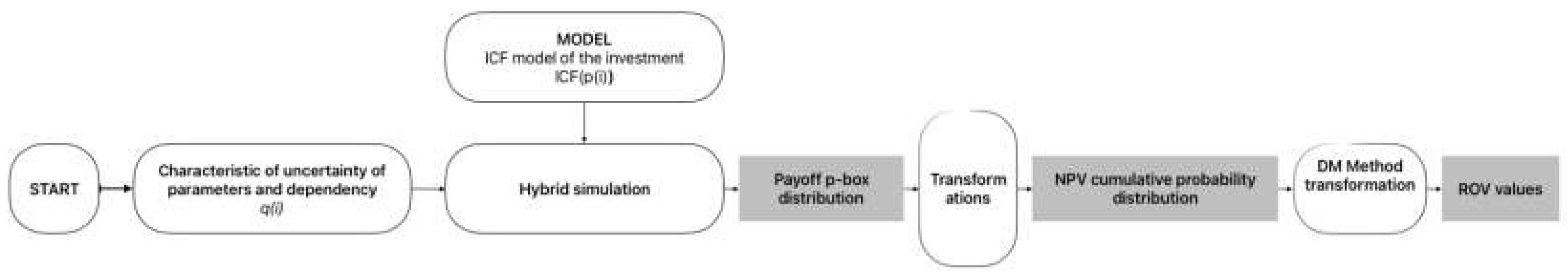
Figure 3.
Net Present Value (NPV) p-box of the investment project for the construction of a new organic-coated sheet plant: (a) considering interdependencies between parameters; (b) assuming independence between parameters.
Figure 3.
Net Present Value (NPV) p-box of the investment project for the construction of a new organic-coated sheet plant: (a) considering interdependencies between parameters; (b) assuming independence between parameters.
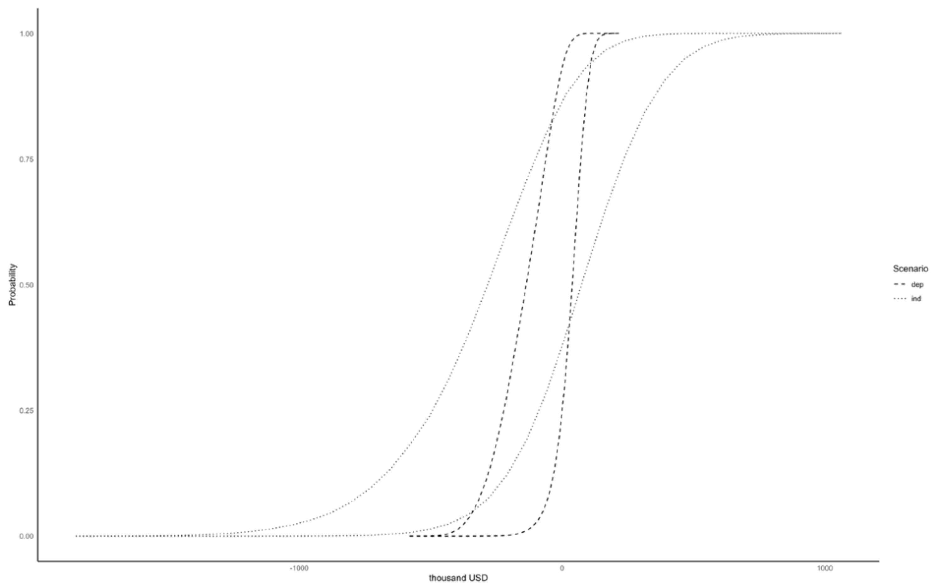
Figure 4.
Comparison of NPV pay-off functions for credibility, ambiguity and pignistic transformations.
Figure 4.
Comparison of NPV pay-off functions for credibility, ambiguity and pignistic transformations.
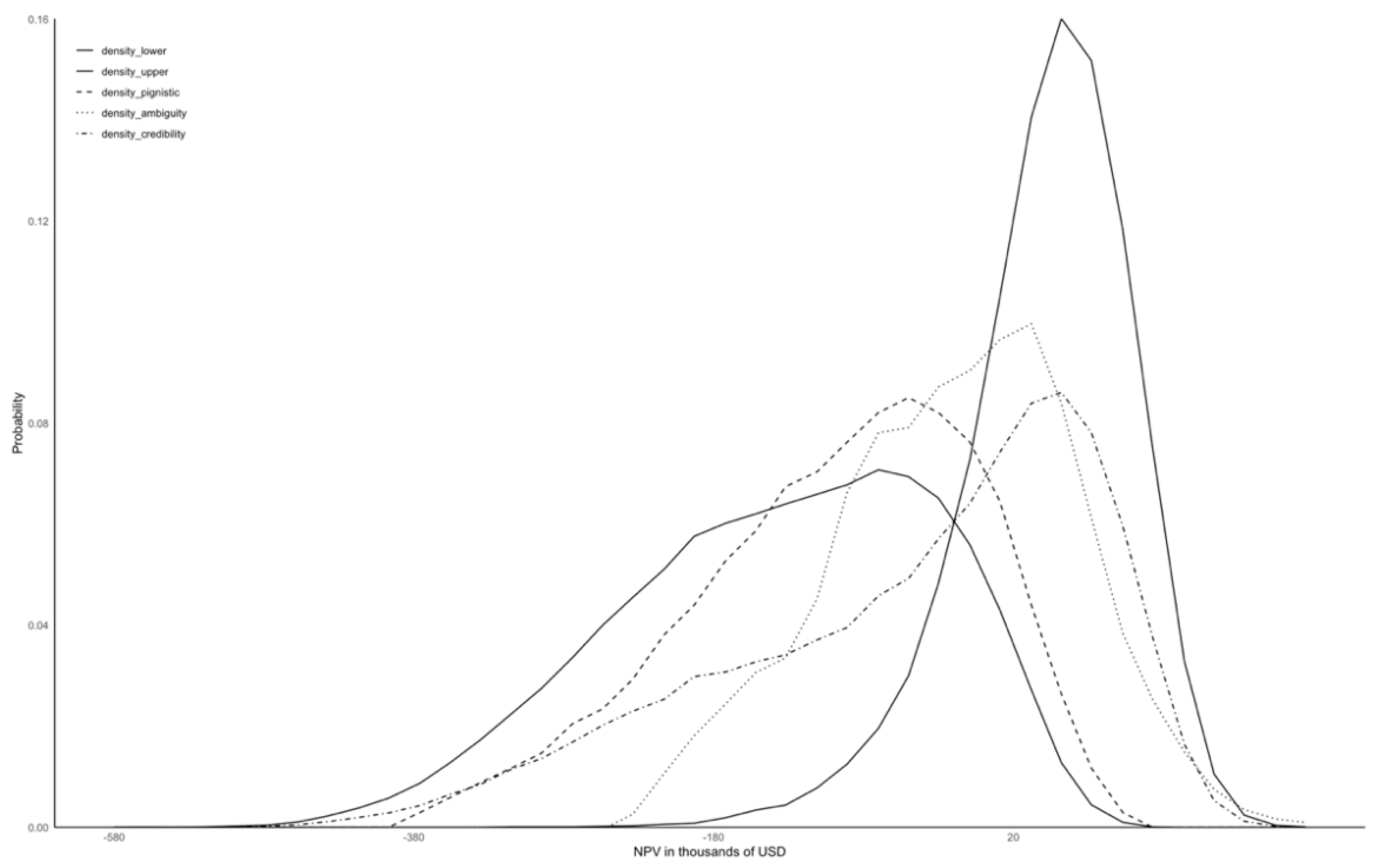
Figure 5.
Transformation of the NPV p-box into subjective cumulative payoff distributions: comparison of pignistic, ambiguity (λ = 0.5), and credibility (β = 0.5) approaches.
Figure 5.
Transformation of the NPV p-box into subjective cumulative payoff distributions: comparison of pignistic, ambiguity (λ = 0.5), and credibility (β = 0.5) approaches.
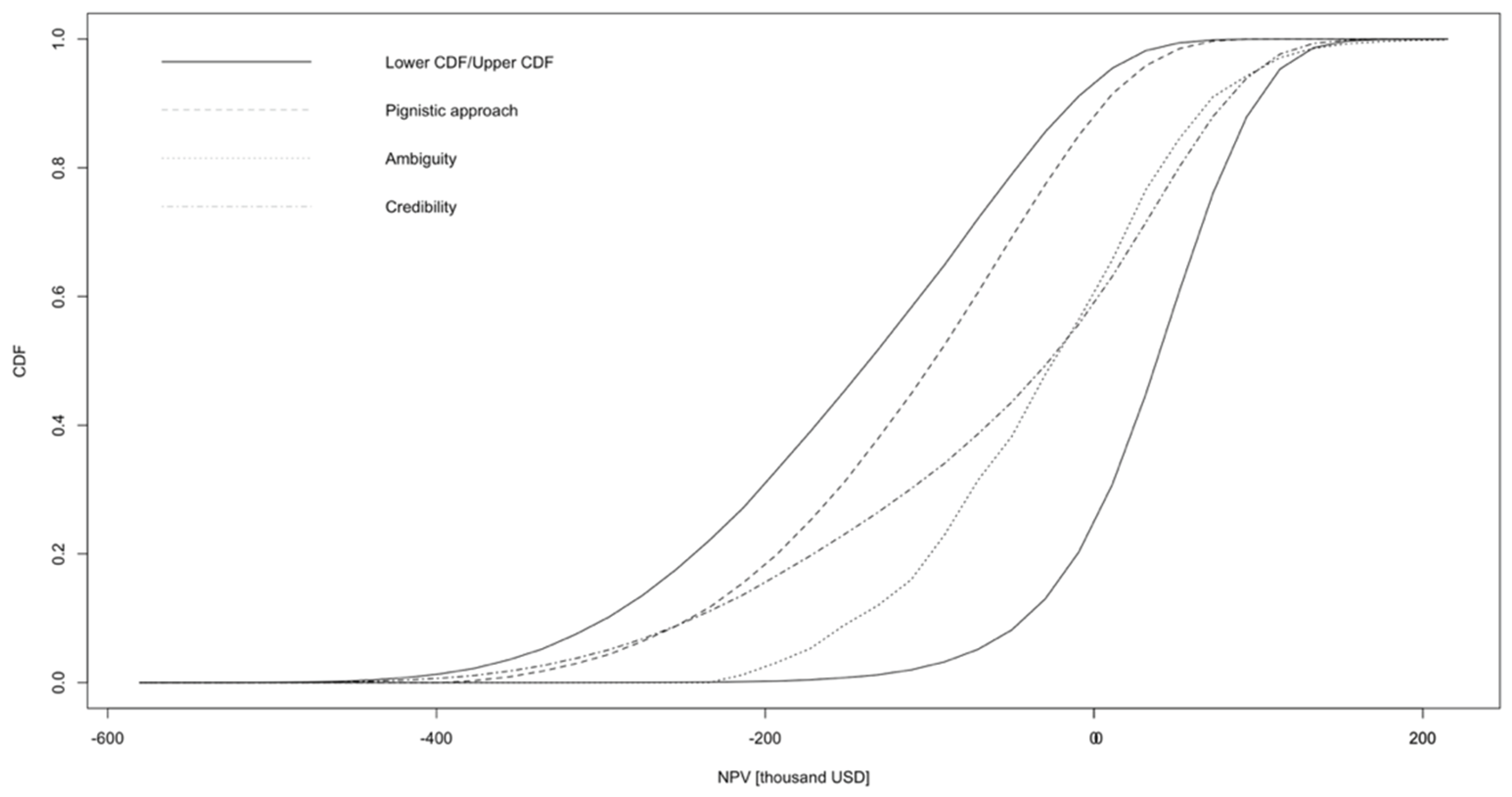

Table 1.
Notation for Parameters and Variables Used in NPV Calculation
|
Indices t – investment period: {1,…,T}, scen – scenario: base - baseline, inv – investment, prod – product: OC – oc sheet, HDG – hdg sheet, CR – cr sheet, scrap – scrap, Input parameters TA – tax, - capacity of prod plan, – market share of prod product, DTR – receivable turnover ratio, CTR – cash turnover ratio, ITO – inventory turnover ratio, DTP – payable turnover ratio, PUCprod – per-unit consumption of sheet required to produce prod sheet, - fixed cost of prod plan, - other annual variable production costs per ton for prod sheet, Auxiliary variables - profit after tax in scen scenario in t, – annual depreciation of prod plan in t - the change in net working capital in scen scenario in t, - residual value in scen scenario in T, - revenue in scen scenario in t, - total cost in scen scenario in t, – sales volume of prod product in scen scenario in t, – net working capital in year t in scenario scen, - cost of CR sheet per ton of prod sheet in year t, - sales forecast for prod product, Uncertain variables – price of prod per ton in year t, – apparent consumption forecast for prod product in t. |
Table 2.
Correlation matrix for products prices
| Scrap | CR sheet | HDG sheet | OC sheet | |
|---|---|---|---|---|
| Scrap | 1.000 | 0.955 | 0.892 | 0.853 |
| CR sheet | 0.955 | 1.000 | 0.961 | 0.921 |
| HDG sheet | 0.892 | 0.961 | 1.000 | 0.911 |
| OC sheet | 0.853 | 0.921 | 0.911 | 1.000 |
Table 3.
Interval-regression coefficient capturing the interdependence between drift parameters of the individual product-price series
Table 3.
Interval-regression coefficient capturing the interdependence between drift parameters of the individual product-price series
| Independent variable | Dependent variable | ||||
|---|---|---|---|---|---|
| Scrap | CR sheet | HDG sheet | OC sheet | ||
| Scrap | a1 | [-0.060; 1.943] | [0.369; 1.378] | [0.589; 1.554] | |
| a2 | [-0.018; 0.001] | [-0.006; -0.002] | [0.003; 0.0098] | ||
| CR sheet | a1 | [-0.897; 2.914] | [-1.611; 3.287] | [-1.689; 3.951] | |
| a2 | [-0.013; 0.041] | [-0.015; 0.039] | [-0.031; 0.069] | ||
| HDG sheet | a1 | [0.721; 1.489] | [0.399; 1.598] | [0.531; 1.811] | |
| a2 | [0.003; 0.006] | [-0.011; -0.003] | [0.004; 0.016] | ||
| OC sheet | a1 | [0.063; 1.689 | [-2.160; 3.866] | [-0.599; 2.112] | |
| a2 | [-0.012; 0.003 ] | [-0.062; 0.040] | [-0.022; 0.007] | ||
Table 4.
Interval-regression coefficient capturing the interdependence between drift parameters of apparent consumption for HDG sheet and OC sheet
Table 4.
Interval-regression coefficient capturing the interdependence between drift parameters of apparent consumption for HDG sheet and OC sheet
| Independent variable | Dependent variable | ||
|---|---|---|---|
| HDG sheet | OC sheet | ||
| HDG sheet | a1 | [-0.239; 0.800] | |
| a2 | [-0.050; 0.167] | ||
| OC sheet | a1 | [-1.589; 3.461] | |
| a2 | [-0.040; 0.088] | ||
Table 5.
Comparison of simulation results and transformations (thousand USD).
| E(npv) | -3.42 USD | 1.05 USD | -2.48 USD | -492 USD | -1.18 USD |
| Std dev | 4.13 USD | 3.16 USD | 3.45 USD | 2603 USD | 3.06 USD |
| Success ratio | 8% | 80% | 15% | 54% | 55% |
| ROV | 2.41 USD | 50.91 USD | 4.60 USD | 23.72 USD | 26.66 USD |
Disclaimer/Publisher’s Note: The statements, opinions and data contained in all publications are solely those of the individual author(s) and contributor(s) and not of MDPI and/or the editor(s). MDPI and/or the editor(s) disclaim responsibility for any injury to people or property resulting from any ideas, methods, instructions or products referred to in the content. |
© 2025 by the authors. Licensee MDPI, Basel, Switzerland. This article is an open access article distributed under the terms and conditions of the Creative Commons Attribution (CC BY) license (http://creativecommons.org/licenses/by/4.0/).
Copyright: This open access article is published under a Creative Commons CC BY 4.0 license, which permit the free download, distribution, and reuse, provided that the author and preprint are cited in any reuse.


