
Submitted:
26 May 2025
Posted:
27 May 2025
You are already at the latest version
Abstract
This paper advances hydrological management by harnessing social media data from Instagram, X, Flickr, and YouTube during Medicane Ianos (September 2020). The dataset included 7,915 texts, 2,949 photos, and 752 videos. Texts were classified into five disaster management categories: Ianos identification, Consequences, Disaster Management, Weather Information, and Emotions/Opinions. Classification used LSTM-RNN and transformers.Photos were categorized as related or unrelated using an ensemble of fine-tuned VGG-19, ResNet101, and EfficientNet models, boosting accuracy. Over 160,000 YouTube and 8,000 Instagram video frames were extracted, analyzed, and assessed via a Relevant Share Video Index (RSVI) to quantify content relevance.Location entity recognition (LER), geoparsing, geocoding, and GIS mapping spatially contextualized the data. Findings reveal that dataset size and classification complexity impact model performance, and custom epoch tuning optimizes accuracy-efficiency balance. LSTM-RNN outperformed transformers on the relatively small corpus. The GR-NLP-Toolkit’s LER performance on medicane texts provides further insights. Lastly, analysis shows most relevant posts appeared during the medicane’s active phase.
Keywords:
deep learning
; hydrological management
; medicane Ianos
; photo classification
; social media
1. Introduction
Since ancient times, crowdsourcing information has been vital for obtaining data for various calculations (Abraham et al. 2024). Stravon mentioned the importance of the latter especially when there are no scientific measurements (i.e. in the absence of instrumental measurements) (Stravon, Geografika, Book B, Mathematical Geography). How many times did the ancient geographers rely on travellers for calculating distances? The answer is really many times. In ancient manuscripts we find that Eratosthenes was mentioning crowdsourcing information obtained by travellers or other people. (Geografika, Book B, Mathematical Geography). In any time period we live in, crowdsourcing contributes to many disciplines as crowdsourced information is instantly reported, contributed, captured and rapidly shared. We could dare to associate the information shared by people in ancient times with the information that is shared nowadays through social media. From a geographical perspective, social media data can be treated as an unconventional source of volunteered geographical information (VGI) (Goodchild 2007) in which the social media users share content, thus unintentionally contributing to related disciplines.
Even with the best of the computer-based measurements of our times though, the fact that billions of people are equipped with a mobile with a very wide range of technological capabilities and the fact that billions of posts are generated daily, social media emerge as a source that cannot be ignored [1,2,3].
On the other hand, it is widely known that the management of environmental problems is a global concern today. Climate change affects us all, and as a result a lot of related initiatives have been added to our lives. The majority of researchers nowadays relate the increase of floods and hydrological hazards to the climatic change (Hirabayashi et al. 2021; Wasko et al. 2021).
As a result, disaster management of hydrological hazards is vital for preventing, mitigating and responding to natural disaster events. Recent technological tools that are utilized in disaster management DM tasks are imagery, drones and social media (Daud et al. 2022; Iqbal et al. 2023).
Specifically regarding the latter in hydrological hazard management, the challenges of manipulating social media data are numerous (Guo et al. 2025). Some of the most significant include the following cases: sharing incomplete information (Abraham et al. 2024); repeating information (Feng et al. 2020); the enormous volume of information (Abraham et al. 2024) produced rapidly (Chen et al. 2023); fake news (Aïmeur et al. 2023; Feng et al. 2020), although these issues are mostly reported in fields of controversial areas, like politics (Allcott and Gentzkow 2017) and not in topics regarding natural disasters and their actual consequences. With regard to floods, social media data are considered an especially effective alternative or a source of added value since survey operations and imagery of high accuracy are costly and software-based solutions are input-dependent (Guo et al. 2025). Generative artificial intelligence (GAI) is expected to worsen the related issues, especially in terms of generating scenario-based flood images.
While some automatically generated metadata of a post are precise enough (i.e a timestamp, embedded geographic coordinates), more generally there is a high level of ambiguity in social media posts as the time and place of the post do not necessarily reflect the actual time and place of the photo (Gao et al. 2011; Feng et al. 2020). Moreover, posts consisting of text, photos, videos or combinations of those are considered in many cases subjective and inaccurate or erroneous (Feng et al. 2020; Abraham et al. 2024; Soomro et al. 2024). Even in natural disasters there are no reports of fake news incidents – at least not intentional – and until the early weeks of 2025, the credibility of social media information, which is a general topic, and the effective manipulation of fake news, which is a special subtopic, are emerging in social media in general, especially with regard to the latter, when there are controversial topics (Petratos and Faccia 2023). There are some initial steps towards defining misinformation in risk response of disaster management, mostly at a qualitative level (Omar and Belle 2024) and various other deep learning-based approaches (Zair et al. 2022). Having different data modalities is a very significant capability, as they can lead to extracting significant in situ information that would not otherwise be tracked, especially when field inspection is not always an option as it requires budget and personnel. And even in those cases where it is possible, rapid field inspection is often a utopian dream (Kanth et al. 2022). Considering all of the above also in relation to the climatic change, social media have emerged as valuable ways of communicating, disseminating news, information, opinions, emotions and other comments suitable for appropriate hydrological management.
A method for measuring the credibility of social media content is similar to the notion of Linus’s Law (Haklay et al. 2010). As in open source computer software, the more programmers the fewer the bugs in the end (Schweik et al. 2008), in social media, when reporting on something really obvious – for example, the appearance of a natural disaster event – the more people mentioning the related information, the more credible the related information is.
Even if the instrumental measurements are more precise and credible, the contribution of social media can be considered, in many cases, invaluable as it can provide information that cannot be captured from satellites, such as instructions from authorities, details about missing people, humanitarian aid, emotional advice, particulars about provision, about planning, even in situ information: e.g. ‘how the clouds look from where I am’, or other comments from local experience comparing, for instance, the current natural event to those of previous times.
There is a lot of research which assesses the contribution of social media to hydrological matters (Section 1.1). In recent years, there is no doubt that there is a tendency for more AI-based approaches (Abraham et al. 2024), which can deal with the enormous volume of the information produced.
Current research presents a methodological framework for extracting crowdsourced hydrological information from a mash-up of social media datasets and of different modalities and specifically, text strings, images and videos collected by using hashtags and keywords regarding the Ianos medicane (Mediterranean, Greek territory, September 2020) from several social media platforms. Moreover, recent trends in AI have been utilized: a comparison of Long Short Term Memory – Recurrent Neural Networks (LSTM-RNN) and transformers for text classification; an ensemble method of location entity recognition (LER) and conventional geoparsing; and an ensemble method among a fine-tuned VGG-19, ResNet101 and EfficientNet for photo classification. The novel ensemble method was used for classifying video frames which were sequentially used for estimating a new index: the Relevant Share Video Index (RSVI), which provides an insight into the extent to which a video contains relevant photo images.
The next sections of the paper present indicative related work
(Section 1.1), and sequentially provide a description of the medicane Ianos (Section 2) and information about the Data and Material Used (Section 2.1). The analytic description of the methodology is in Section 3, while the next Section 4 is related to Results and Discussion. Finally Section 5 completes the research paper with a conclusion.
1.1. Related Work
In the literature, there is a variety of definitions of what can be called a ‘mash-up’ according, apparently, to the field of origin of the researchers. He and Zha (2013) used previously published definitions: ‘easy, fast integration, frequently made possible by access to open APIs and data sources to produce results beyond the predictions of the data owners’ (de Vrieze et al. 2010; Bader et al. 2012).
The definition by He and Zha (2013) is specific to the social media mash-up as a ‘special type of mash-up application that relies on various open APIs and feeds to combine publicly available content from different social media sites to create valuable information and build useful new applications or services’. Inevitably a lot of research associates mash-ups with services (Hummer et al. 2010, Chen and Peng 2012). Apart from services, the term ’mash-ups’ is apparently applied to a variety of cases: among others, we find data mash-ups (Jarrar and Dikaiakos 2009; Fung et al. 2011) and the mash-up of techniques or methods (Fuller 2010; Nakamura et al. 2016) etc.
A general definition of the term mash-up could be ‘Any complementary, simultaneous use of different elements, either datasets, services, methods, or approaches, which produce a result that could not be produced by relying on the used elements individually”. Despite the lack of a precise definition, the importance of mash-ups, in a sense of combining sources, services, techniques, approaches, in crisis situations caused by hydrological disasters is significant.
The effectiveness of social media mash-ups has emerged, among others, in Schulz and Paulheim (2013) who assessed them as a ‘helpful way to provide information to the command staff’. Decision-makers can also benefit. The same authors referred to the significance of social media sources in various cases, including among others the Red River Floods (April 2009, USA). By assessing various other disastrous events, e.g. earthquakes, they concluded that crowds can be used for rapid mapping. A few years later, in 2015, the Copernicus ecosystem (source: https://mapping.emergency.copernicus.eu/) initiated the rapid emergency mapping service, which has been providing valuable insights extracted through the automatic analysis of imagery data.
With regard to hydrological disaster events and data processing, the topic of effective photo classification of such events has been researched in recent years (Ning et al. 2020; Pereira et al. 2020; Romanascu et al. 2020; Kanth et al. 2022). As AI-related solutions are emerging, it is really obvious that those solutions would be assessed in order to confront with various time-consuming and complicated tasks of the field.
A varied performance is demonstrated in the literature regarding classification tasks, ranging from a low to mid performance of the models (Ridwan et al. 2022; Delimayanti et al. 2020) up to more effective solutions, which receive SOTA metrics of above 90% (Ponce-Lopez and Spataru 2022). This is quite logical as there are many different factors that affect the actual SOTA evaluation metric.
Sheth et al. (2024) presented an ensemble method technique based on InceptionV3 and CNN, achieving an accuracy rate of more than 92%. They applied their approach to the CWFE-DB database, containing photos of Cyclones, Wildfires, Floods and Earthquakes. Compared to CNN only, the ensemble technique received a better score in SOTA metrics.
Moreover, Jackson et al. (2023) assessed the performance of 11 models in terms of their ability to classify photos as flood-related and not flood-related. The dataset used was FloodNet. The dataset provides Unmanned Aerial System (UAS) images, so it might not be so relevant to social media-posted photos. However, even though they are not the majority, similar photos are frequently posted on social media.
Pally and Samadi (2022) assessed the performance of a CNN model, developed by them, for flood image classification and object-detection models for object detection in flood-related images, including Fast R-CNN and YOLOv3. One conclusion, among others, is the very varying performance of different algorithms on different objects of the same dataset.
In (Soomro et al. 2024) the effectiveness of X, formely Twitter, was assessed, when contributing to flood management. They emphasized on the emotional and public opinion perspective available through X for hydrological management. They processed all the related tweets of the Pakistan floods of 2022 in Karachi. They scored the sentiment of each tweet based on a lexicon-based sentiment assessment approach.
They assessed the Twitter findings along with output from other sources, characterizing social media data and Twitter as crucial for resilience, the sharing of information and the adaptation of the announcements of the public authority.
Kanth et al. (2022) presented a deep learning approach for flood mapping based on social media data. They classified text and photos with an accuracy of 98% for a pretrained and fine-tuned Bidirectional Encoder Representations from Transformers (BERT) and a range of 75–81% accuracy from various deep learning models for photo classification. They assessed their approach on three different flood events: the floods in Chennai 2015; Kerala 2018; and Pune 2019. They initially classified the texts as I. Related to floods and II. Not related to floods and then the ‘flood texts’ were further processed along with their corresponding images and classified into three main categories: I. No flood; II. Mild; and III. Severe. They assessed various machine learning models: SVM, ANN, CNN, Bi-LSTM and BERT for text classification and ResNet, VGG16, Inception V3 and Inception V4 for photo classification.
Moreover, in (Du et al. 2025) CA-Resnet was presented, which is an approach based on Resnet with an addition of Coordinate Attention on it, for identifying water-depth estimation from social media data. They tested their approach on a flood dataset of photos posted on social media regarding the 2021 Henan rainstorm in China, which consisted eventually of 5676 images. Their approach, in comparison to the conventional VGGNet, ResNet, GoogleNet and EfficientNet had a slightly better performance measured by the F1, Precision, Recall, and MAE, while their approach was outperformed slightly by another model only with regard to Accuracy. In their research, social media datasets emerge as a valuable source for obtaining water-depth data from different modalities at zero cost.
The water level as a matter of classification was also formulated in Feng et al. (2020). Their approach included initially classifying images posted through social media, as ‘related’ and ‘not related’ to flood, while the related ones with the presence of people were further processed in order to classify the water level in respect to various parts of the human body that were submerged in the flooded water. As a case study they used Hurricane Harvey (2017). They used the DIRSM dataset extended by photos from other sources and consisted of 19,570 features. In general, their approach consisted of using various models, had little better precision and average precision scores calculated in cut-offs in comparison to previous approaches that had been applied during the MediaEval ’17 workshop. With regard to the estimation of water levels, the overall accuracy of their approach has impressively better metrics (overall accuracy of 89.2%), while by fusing their model with that of another method they achieved an overall accuracy of 90%. Finally they mapped the flooded area, by extracting the location of social media, and by using census administrative areas. They also manipulated the data with other sources, like remote sensing. By combining social media and remote sensing there was an increasing accuracy. One of the noted assumptions of combining remote sensing and social media is that the latter can contribute to identifying the severity of an event at an earlier time point.
Guo et al. (2025) assessed the contribution of social media to flood-related disasters by analysing posts from 2016 up to 2024 regarding urban flooding in Changsha, a city in South Central China, which is affected by flood events resulting from, among other factors, rapid urbanization, heavy rainfall, low topography and the Xiangjiang river. Their approach includes methods for extracting information from text and photos. Related information included flood locations and water depths. They also found positive correlation among the volume of the generated posts and various indicators, including population and seasonal rainfall. They performed the analysis within a prisma of a short-term and a long-term calendar time periods. During the first period, the posted information mostly relates to the response, while during the second period, the posts are concerned with prevention and governmental responsibilities. Yolo v5 was used for extracting information from photos. Other research is also available that deals with, among others, the potential of social media to contribute to identifying urban waterlogging (Chen et al. 2023).
2. Case Study: Medicane Ianos
Ianos was as a barometric low with tropical characteristics (source: National Observatory of Athens (NOA); meteo.gr). While the actual medicane formulation started on September 17 (Lagouvardos et al. 2020; Lagouvardos et al. 2022), the cyclone was formed as a surface cyclone in the Gulf of Sidra on September 15, while its original development started even earlier, somewhere during September 11–12. Its trajectory was from the north coast of Africa, in Libya, towards the north. During September 16, the medicane was located between Sicily and Greece, and thus affected the Greek territory from September 17, the date that is was formed as a medicane (Lagouvardos et al. 2022), to September 19 with an inverted u trajectory from the Ionian Sea to the south of Crete, ending its 1900 km journey on the Egyptian coast during September 20. Sea surface temperature (SST) was more than 28 ¼C in the Gulf of Sidra while along the route of the medicane the SST has a range of more than 2 ¼C (Lagouvardos et al. 2022).
The rainfall in some cases was more than 300 mm (Pertouli, West Thessaly, Greece; source: NOA and meteo.gr), and more than 350 mm (Cephalonia island, NOA), while in West Greece in general the daily accumulated rainfall was over 600 mm. The minimum sea level pressure (SLP) was 984.3hPa, recorded in Palliki, Cephalonia, while the station in Zante recorded 989.1hPa, and a mean wind speed of 30 m s−1, with wind gusts reaching a maximum of 54 m s−1. The whole Greece and other neighboring countries including Turkey and Bulgaria were reported to have even noticed even a small effect of the medicane (source: Daily Press and Social Media reports).
Among the consequences of the medicane were numerous landslides, flooding and precipitation. Lagouvardos et al. (2022) identified more than 1400 landslides caused in two days. Four casualties and damage to numerous properties and infrastructure composed a disastrous landscape.
The medicane was named by the NOA. Other names referred to in various sources include Cassilda, Udine and Tulpar. Ianos was the fourth medicane since 2016, after medicane Trixie, Medicane Numa (November 2017) and Medicane Zorbas (September 2018) (Lagouvardos et al. 2022).
2.1. Data and Material Used
A mash-up consisting of the following datasets was created:
An Instagram dataset scraped during 2020 (Arapostathis, 2020), which, after processing, consisted of 241 videos and 1414 photos and related text strings, posted from September 12 up to September 21, 2020.
An X dataset, consisting of 4,867 tweets, scraped during July 2024, using the application twibot v 1.4.6 and posted from September 12 2020 up to October 30, 2020.
A Flickr dataset, consisting of 1,535 photos with their related metadata which included timestamps, captions, IDs. The Flickr dataset was collected by using the official Flickr Application Programmable Interface (API), posted from September 12 up to October 30, 2020.
A YouTube dataset consisting of 512 videos and their related titles, descriptions and timestamps by employing the official API collected using the keywords: ‘medicane Ianos’ in Greek (κυκλώνας Ιανός ) and English.
The Deucalion dataset (Arapostathis 2024) used for fine-tuning VGG-19, ResNet101 and EfficientNet.
The main language used in the current research was Python. Indicative libraries used were, among others, the torch, transformers, torchvision, gr-nlp-toolkit, ultralytics and pandas. LibreOffice and Quantum GIS were used for quality checks and for developing the final figures and maps, respectively.
3. Methodology
Methodology was organized into five main parts (Figure 1). The first part was related to data collection, followed by the preprocessing of data from all modalities, which included among others the translation of the text strings that were not in Greek. Training text and photo/video models were the third and fourth parts, respectively. Part five was related to location entity recognition (LER) and all the related tasks for map creation. Finally, the presentation of the results completes the components of the current approach.
3.1. Data Collection
As already mentioned, various datasets of different modalities were used in the current research (Figure 2). The Instagram dataset was scraped during 2020, after the occurrence of the Ianos medicane (Arapostathis 2020). The scraping of that time and the Instagram graph API up to the first weeks of 2025, in general, did not provide any specific parameters for defining the exact time period, apart from a ‘recent media’ endpoint. As a result, a lot of noise, consisting of posts shared previously, was accumulated.
The X (former Twitter) dataset was collected during July 2024 through the use of the Twibot app, while for Flickr and YouTube data two scrapers written in Python were created for that purpose.
The time period of interest for X, Flickr and YouTube was extended up to October 30, assuming that potentially some information regarding restoration and disaster management after the flood occurrence would appear, even though in many cases reference has been made to social media users tending to post during the flood occurrence and not afterwards (Soomro et al. 2024).
3.2. Preprocessing
Preprocessing was related to organizing the data from all sources together but for each one of the modalities separately. The text strings of Instagram, X, Flickr and YouTube (both title and description) along with the corresponding timestamps, and various IDs of the associated data (i.e. photo ids, video ids) were bound into a single data frame comprised of 7915 strings.
Processing included the translation of non-Greek texts, excluding the translation of hashtags, the removal of urls, the conversion to lowercase and the removal of various characters like dots and emojis. The translated and processed text strings were then ready for training the deep learning models.
Secondly the photos of Instagram and Flickr were bound into a single folder. Especially regarding Instagram, it should be stated that a caption was associated with more than one of the photos, while in some cases instead of photos there were videos. Some frames were extracted from the videos in order to enrich the photo dataset, while the video files were accumulated in a separate folder along with the YouTube videos.
Finally, with regard to the YouTube and Instagram videos, those were further processed for extracting frames at fps=1 sec. The .jpg formatted frames were then stored at a separate folder, all of them with a filename suitable for associating the frames with the rest of the data in the event of that need (e.g texts).
3.3. Classification
LSTM-RNN, a type of neural networks which are not feed-forward,and transformers were employed for text classification (Figure 3). As previously mentioned, the classification schema was consisting of five classes (Table 1): I. Identification; II. Consequences; III; Tracking and Disaster Management; IV. Weather/Meteo Info.; and V. Emotions, Opinions and Other Comments. There was a long-term experimentation to define the parameters for both models. The final parameters are presented in the results section, where, among other, the importance of the dataset in the actual performance is emphasized. For that purpose, in order to select the appropriate classifier SOTA metrics of LSTM-RNN and transformers were compared, trained in two different training datasets. The first consisted of approximately 10% of the data, and the second of approximately 15%. The training datasets (further split-ed to the size of 90% for training and 10% for testing) of the text strings were generated by using the sample method in python, and each entity was assessed and classified manually and according to the classification schema (Table 1). It is worth mentioning that that classification schema used was a theoretical concept and was not defined for extracting info as an input to hydrological models, but rather for assessing the performance of various classifiers, with various parameters when those are utilized in less straight-forward tasks. One aspect that is worth mentioning custom epoch values were considered, based on the balance between Training Accuracy and Validation Accuracy, thus avoiding over-fitting. In other words, even if Training Accuracy was up to 100%, the appropriate balance ensures more ‘compatible’ training. Therefore, the selected epoch in all of the related graphs in the results section is indicated with a star.
For photo classification, a VGG-19 model was fine-tuned for classifying the related photos in two main classes: 1. Related and 2. Not related to Ianos. As previously mentioned, the dataset used was the Deucalion (Arapostathis S. G. 2024), enriched with various photos of current sources. The version of Deucalion dataset used, was consisted of 2,463 photos which are related to the flood and 2,579 photos classified as not related. As per text classification, the training dataset was splited to training dataset – validation dataset in a ration of 90% - 10%. The origin of the photos is defined within the related reference (Arapostathis S. G.) and it is a mashup of various sources, including a subset of the Instagram’s source used described in (Arapostathis 2020). It is worth mentioning that no specific moderations were applied to the training dataset for classifying the video frames. The enriched version of Deucalion was also used for fine-tuning a ResNet101, along with an EfficientNet model in the same binary classification. As per text classification, the appropriate models were selected by considering the balance between Training accuracy and Validation accuracy. In other words, if the difference of the two metrics was more than a specific threshold then the model was not saved and was not used. Therefore, as per text classification models, the epoch in which the model was saved is indicated with a star.
Videos were processed as a set of photos extracted at an analogy of 1 fps. Based on that set of photos, the Relevant Share Video Index (RSVI) was defined and estimated. RSVI was estimated by estimating the proportion of relevant frames to the total ones, at step k, which is the value of extracted frames per second. In our case, as already mentioned, this was set to 1 second.
Upon extracting the frames from all videos and classifying them through the ensemble method, RSVI was estimated. The actual interpretation of current index is that the bigger the value of the RSVI and more related frames existed in the set of extracted frames.
Ensemble approach: The 3 guessers: Probabilities scenario
In that section the essential theory on which the ensemble method is based on, is described. The approach makes use of three different models (Figure 4). Let’s assume that there are three guessers. Guesser A guesses with an accuracy P1while Guesser B guesses with an accuracy of P2. Finally, guesser C guesses with an accuracy of P3. The probability of having only one guesser having a correct guess is defined as:
pi: The probability that the 1st, 2nd, 3rd, respectively predicted correctly.
1-piis the probability that the i-th predicted wrongly.
The probability of having one guesser correct and the two other wrong is estimated as:
while the percentage of having correct output by considering at least the two-thirds is estimated as:
pi= the probability of i-th voter to be correct
q1= 1 – pi, the probability of the i-th voter to be wrong
P(at least 2 correct)= p1 p2q3 + p1q2p3 + q1p2p3 + p1p2p3
This approach actually describes the estimation of the accuracy of the ensemble method based on a voting system, in which each voter has a value of one as long as the voter’s Acc > 0.5. Since all the guessers in our case received accuracy of more than 50%, the vote of the two, either estimating the sum of weights or each one as one, is the majority. So, in the current case, the approach considers as always correct the decision of at least the two-thirds of the guessers. In our case it could be said that the classifiers are assigned the role of those briefly described “guessers”. In (3) it is assumed that errors are uncorrelated between models (Grinstead and Snell 1997). In practical cases, actual ensemble performance may vary depending on error correlation, which is not directly measured in this current research.
3.4. Location Entity Recognition (LER) and GIS Processing
A transformer pretrained in Greek, was used, available through the GR-NLP-Toolkit (Loukas et al. 2024) for detecting location in the text corpus of the mash-up. An ensemble method was applied using conventional geoparsing as well as for increasing the accuracy of the model. The detected geolocations were geocoded by using commercial geocoding APIs while they were processed in a GIS environment, including filtering of the geocoded locations within the geographic area of interest (GAOI).
4. Results – Discussion
Table 2 and Table 3 present the parameters used for the training of the LSTM-RNN and transformer models. Summarizing, 10 LSTM models and 10 transformer models were trained, performing binary classification for 5 main categories, experimenting with training datasets of two different sizes. It is worth mentioning that the custom epoch was used for selecting the best model in terms of performance, ensuring in parallel that there are no over-fitting issues.
In general, the defining of the appropriate set of parameters is widely discussed, while avoiding over-fitting should always be considered. The custom epoch approach of the current research was based on a logical validation: save the model with the best validation accuracy considering that the absolute difference between training accuracy and validation accuracy should not be more than 10%. Based on that rule, in the following figures the epoch that met the logical rule is indicated with an asterisk. Figure 5, Figure 6, Figure 7, Figure 8, Figure 9, Figure 10, Figure 11, Figure 12, Figure 13 and Figure 14 display the epoch selected as the most effective fine-tuned Transformer, along with the loss and accuracy values for both training and validation, for the smaller and the larger training datasets respectively. Moreover, Figure 15, Figure 16, Figure 17, Figure 18, Figure 19, Figure 20, Figure 21, Figure 22, Figure 23 and Figure 24 display the same info, but for the LSTM-RNN models, for the smaller and larger training datasets respectively.
As can be seen, LSTM-RNN outperformed Transformers in the majority of the metrics in both experiments. The first one was built by using a sample of approximately 10% of the total volume, while the second time the sample was 15% (Table 4). Apart from the actual metrics, LSTM-RNN took much less time to become trained in new equipment, a vital factor considering the relatively small size of the big dataset. Apart from promoting LSTM-RNN to a more suitable classifier for the needs of the current research, it can also be noticed that the bigger the training dataset the better the results in general, or in some cases they are slightly worse. Mean increase of validation accuracy for the LSTM-RNN was 3.6% while for the Transformers it was 4.2%; the maximum decrease was 4% and 3%, respectively, and the maximum increase was 10% for both. The above result is more or less compliant with published research (Ezen-Can 2020; Reusens et al. 2024). Sequentially, the training procedure was iterated by using the LSTM-RNN classifier, enriching the training dataset each time by adding the most significant errors found during the evaluation of each round. After one iterations, the SOTA metrics of the predicted output were improved as it can be seen in Table 5. That finding is more or less consistent with previous findings of the author (Arapostathis 2021) who had found that by iterating the procedure and feeding the model with corrected mistakes the SOTA metrics incrase. The latter was justified for various machine learning models, including SVM.
As already mentioned, the three fine-tuned models were used in order to predict the classification of all the social media images available. The validation accuracy of VGG-19 and ResNet101 was 0.94 and 0.95, respectively, while EfficientNet was 0.93. By using the ensemble approach, considering the voting method, the actual accuracy estimated by using the actual accuracy can reach 0.99 according to the theoretic approach. Prediction accuracy, the metric estimated from the prediction data, was 0.69 for VGG-19 and Resnet101 and 0.69 for efficientNet. The ensemble approach’s accuracy is increased (Table 6). It is important to note that some correlation exists among the indices, which implies that the combined accuracy gained by calculating these specific values using the probability formula (Table 6) might be slightly overestimated compared to treating all indicators as fully independent. Therefore, while the direct calculation suggests a 10-15% increase in accuracy, a more realistic estimate, accounting for interdependencies, would be around 5%. This subtle adjustment reflects the complexity of the data and strengthens the robustness of the analysis by acknowledging inherent correlations.
This statement is further empirically supported by the calculation of corresponding indices for the YouTube frames (Table 7), where the observed accuracy gains were lower, approximately 3% and 2%, respectively, reinforcing the effect of interdependencies in real-world data. In general, in the literature there are approaches indicating that the use of many models for a image classification provide better results (Tseng et al. 2023; Bashar et al. 2025)
4.1. Video frames Classification
Video frames’ classification is a quite controversial procedure. Apart from the obvious positives and negatives, there are many cases that are actually at the discretion of the researcher and their expectancy and belief of what should be classified as True or False. For instance, video frames without any actual information but with two journalists speaking about the effects along with a text caption mentioning the medicane. According to the needs of a research, a model might identify those as related or not related. On the other hand, in the case where actual information is needed, the referred photos should be excluded from the actual output. In that case the RSVI value can be more more critical for interpreting as how many actual views appear in a video excluding any other information, such as ‘headlines’ etc. In general, in the event of multi-class classification the RSVI value can be estimated for each one of the classes providing thus invaluable information for each video separately or a set o videos. Considering the latter, the VGG-19 and ResNet101, trained on the Deucalion dataset and a few additions, were able to obtain 0.69 and 0.73 prediction accuracy, respectively, while EfficientNet was estimated at 0.75, all for youtube frames. The prediction accuracy of the ensemble method was 0.77, very nice considering the volume of the related information. Regarding Instagram frames, the prediction accuracy of VGG-19 was 0.80, and of ResNet101 0.81. EfficientNet’s accuracy was 0.79, while the prediction accuracy of the ensemble method was 0.82 (Table 7). The results can be considered impressive especially when acknowledging the fact that the models did not use YouTube frames for training. That fact is an empiric validation of appropriate calibration (Figure 5, Figure 6, Figure 7, Figure 8, Figure 9, Figure 10, Figure 11, Figure 12, Figure 13, Figure 14, Figure 15, Figure 16, Figure 17, Figure 18, Figure 19, Figure 20, Figure 21, Figure 22, Figure 23 and Figure 24), ensuring that there are no significant over-fitting issues. Always when interpreting the SOTA metrics though the researchers should always consider various factors, including e.g. the complexity of the classification schema and the volume of the dataset.
The mean RSVI of the 160,161 frames extracted from 511 videos was 0.34, a useful metric – especially when dealing with videos of various topics. One of the videos was excluded due to its length: It was more than 11 hours and was about a simulation. Moreover the Mean RSVI of the 241 Instagram videos was 0.548 (Table 8). Instagram videos seem to have more related content, while it could be empirically stated that there is the possibility of extracting more in-situ and timely information, in contrary to YouTube which has, among other, videos of larger length.
4.2. Location Entity Recognition and GIS Processing
In Table 10 and Table 11 the SOTA metrics of LER and combined LER and geoparsing procedures. The BERT-based pretrained in Greek Transformer had a relatively nice Accuracy and Precision, which was significantly increased upon GIS processing. It should be stated that fine-tuning the Greek-based BERT Transformer would not be a logical decision as the total volume of the text strings is relatively low for these kinds of tasks.
Geocoding included the use of commercial Geocoding APIs who assigned decimal geographic coordinates to the related entities. The output was also processed in the GIS environment.

Table 9.
SOTA evaluation of Location Entity Extraction. One Round of Additions.
| Specificity | F1 | Recall | Accuracy | Precision | N = 200 rows, 476 cases |
|---|---|---|---|---|---|
| 0.58 | 0.9 | 0.93 | 0.85 | 0.88 | LER |
| 1 | 0.95 | 0.91 | 0.93 | 1 | LER + Geoparsing |
Table 10.
Geocoding Evaluation.
| Accuracy | N = 100 |
|---|---|
| 0.99 | GIS Analysis, conventional geocoding APIs |
4.3. Actual output of the models in graphs and maps
Figure 25 displays the frequency of posts per category and per time period. The time intervals were 24 hrs starting from September 11, 2020 at 01:24:35 GMT. As can be easily seen, apart from Instagram source which includes data posted until September 21, the vast majority of the posted content was during the actual occurrence of the event, an outcome verified in the literature in similar cases [2]. X is dominating in terms of frequency, while it can be mentioned that all the social media types follow the same pattern, having a volume- pick during the actual unfold-ness of Ianos (Figure 25). The latter is compatible with literature’s findings (Soomro et al. 2024). Moreover DM class, as described in Table 1 prevails in terms of frequency, followed by weather info and emotions. In general, emotions, consequence-tracking and identification info seem to have more or less similar frequency.
Figure 26 displays a tiny sample of the photos that were processed through the current approach. In general, it should be stated that relying exclusively on photos could sometimes be proven risky. Even a photo of, for example, weather conditions of a specific place can be a valuable piece of in situ information, especially when the timestamp is the actual time of the photo capture; however, there is a lot of uncertainty as social media users tend to repost photos and at the same time describe a situation at their place in text. Moreover, GAI is expected to worsen the landscape with artificial images, none of which can one be assured on how ‘real’ they may seem in the next few years. In this current research there were no fake news problems identified, the related topic along with the GAI dimension should be researched in the future.
Finally, Figure 27 and Figure 28 display two maps with the geocoded locations recognized in the text strings and filtered in the geographic area of interest. The first map clusters the nearby geocoded points while the second one displays the source categories of the data: red for YouTube; black for X; purple for Instagram; and green for Flickr.
5. Conclusion
The current approach is dedicated to the notion of data mash-ups from unconventional VGI sources, and effective processing for extracting information suitable for disaster management procedures. State-of-the-art approaches, including LSTM-RNN, transformers, fine-tuned VGG-19, REsNet101 and EfficientNet along with Named Entity Recognition (NER) BERT-based models were employed for the analysis. The case study used was the medicane Ianos, which affected Greece during September 2020. The sources were of three modalities. Through the current approach it was possible to extract thousands of related images and geolocations and text strings accumulated in various categories useful for DM purposes. Moreover, the classification of photos provides valuable insights that cannot be described in a few words while the RSVI is useful, especially when dealing with videos of various topics.
Apart from its research value, the current output can be used for various operational phases of tracking and mitigating hydrological disasters, while it can also be a basis for an approach that will be able to visualize and classify related content in real time. Future steps of the research could include a focus on more applied and operational output, in terms of compatibility to conventional hydrological models and operational procedures. Various scripts of the approach, written in Python along with some sample of anonymized data can be found at author’s github: github.com/stathisar
Acknowledgments
“During the preparation of this manuscript/study, the author(s) used [ChatGPT various versions available from October 2025 up to May 2025] for purposes of technical support in python, invaluable assistance since the author, in programming, is an R expert and recently started (time period of one year) using Python more extensively. The author has reviewed and edited the output and take full responsibility for the content of this publication.“
References
- Abraham, K.; Abdelwahab, M.; Abo-Zahhad, M. (2024). Classification and detection of natural disasters using machine learning and deep learning techniques: A review. Earth Science Informatics, 17(2), 869-891.
- Soomro, S.; Boota, M.W.; Zwain, H.M.; Shi, X.; Guo, J.; Li, Y.; Tayyab, M.; … & Yu, J. (2024). How effective is twitter (X) social media data for urban flood management?. Journal of Hydrology, 634, 131129.
- Du, W.; Qian, M.; He, S.; Xu, L.; Zhang, X.; Huang, M.; Chen, N. (2025). An improved ResNet method for urban flooding water depth estimation from social media images. Measurement, 242, 116114.
- Aïmeur, E.; Amri, S.; Brassard, G. (2023). Fake news, disinformation and misinformation in social media: A review. Social Network Analysis and Mining, 13(1), 30.
- Allcott, H.; Gentzkow, M. (2017). Social media and fake news in the 2016 election. Journal of Economic Perspectives, 31(2), 211-236.
- Arapostathis, S.G. (2020, December). The Ianos Cyclone (September 2020, Greece) from the Perspective of Utilizing Social Networks for DM. In International Conference on Information Technology in Disaster Risk Reduction (pp. 160-169). Cham: Springer International Publishing.
- Arapostathis, S.G. (2021). A methodology for automatic acquisition of flood-event management information from social media: The flood in Messinia, South Greece, 2016. Information Systems Frontiers, 23(5), 1127-1144.
- Arapostathis, S.G. (2024). Deucalion: A dataset for flood related research. In OSF PrePrints.
- Bader, G.; He, W.; Anjomshoaa, A.; Tjoa, A.M. (2012). Proposing a context-aware enterprise mash-up readiness assessment framework. Information Technology and Management,13(4), 377-387.
- Bashar, M.; Monjur, O.; Islam, S.; Shams, M.G.; Quader, N. (2025). Exploring Synergistic Ensemble Learning: Uniting CNNs, MLP-Mixers, and Vision Transformers to Enhance Image Classification. arXiv preprint. arXiv:2504.09076.
- Chen, Y.; Peng, Y. (2012). A QoS aware services mash-up model for cloud computing applications. Journal of Industrial Engineering and Management, 5(2), 457-472.
- Chen, Y.; Hu, M.; Chen, X.; Wang, F.; Liu, B.; Huo, Z. (2023). An approach of using social media data to detect the real time spatio-temporal variations of urban waterlogging. Journal of Hydrology, 625, 130128.
- Daud, S.M.S.M.; Yusof, M.Y.P.M.; Heo, C.C.; Khoo, L.S.; Singh, M.K.C.; Mahmood, M.S.; Nawawi, H. (2022). Applications of drone in disaster management: A scoping review. Science & Justice, 62(1), 30-42.
- Delimayanti, M.K.; Sari, R.; Laya, M.; Faisal, M.R.; Naryanto, R.F. (2020, October). The effect of pre-processing on the classification of twitter’s flood disaster messages using support vector machine algorithm. In 2020 3rd International Conference on Applied Engineering (ICAE) (pp. 1-6). IEEE.
- de Vrieze, P.; Xu, L. & Xie, L. (2010). Encyclopedia of E-Business Development and Management in the Digital Economy. Hershey, Pennsylvania: Idea Group Publishing, Situational Enterprise Services.
- Ezen-Can, A. (2020). A Comparison of LSTM and BERT for Small Corpus. arXiv preprint. arXiv:2009.05451.
- Feng, Y.; Brenner, C.; Sester, M. (2020). Flood severity mapping from Volunteered Geographic Information by interpreting water level from images containing people: A case study of Hurricane Harvey. ISPRS Journal of Photogrammetry and Remote Sensing, 169, 301-319.
- Fuller, J.; COMSYS LLC, P. (2010). Mashups Can Be Gravy: Techniques for Bringing the Web to SAS®. https://support.sas.com/resources/papers/proceedings10/016-2010. Available online: https://support.sas.com/resources/papers/proceedings10/016-2010.
- Fung, B.C.; Trojer, T.; Hung, P.C.; Xiong, L.; Al-Hussaeni, K.; & Dssouli, R. (2011). Service-oriented architecture for high-dimensional private data mashup. IEEE Transactions on Services Computing, 5(3), 373-386.
- Gao, H.; Barbier, G.; Goolsby, R. (2011). Harnessing the crowdsourcing power of social media for disaster relief. IEEE Intelligent Systems, 26(3), 10-14.
- Goodchild, M.F. (2007). Citizens as sensors: The world of volunteered geography. GeoJournal, 69, 211-221.
- Grinstead, C.M.; Snell, J.L. (1997). Introduction to probability. American Mathematical Society. https://math.dartmouth.edu/~prob/prob/prob. Available online: https://math.dartmouth.edu/~prob/prob/prob.
- Guo, Q.; Jiao, S.; Yang, Y.; Yu, Y.; Pan, Y. (2025). Assessment of urban flood disaster responses and causal analysis at different temporal scales based on social media data and machine learning algorithms. International Journal of Disaster Risk Reduction, 117, 105170.
- Haklay, M.; Basiouka, S.; Antoniou, V.; Ather, A. (2010). How many volunteers does it take to map an area well? The validity of Linus’ law to volunteered geographic information. The Cartographic Journal, 47(4), 315-322.
- He, W.; Zha, S. (2014). Insights into the adoption of social media mashups. Internet Research, 24(2), 160-180.
- Hirabayashi, Y.; Alifu, H.; Yamazaki, D.; Imada, Y.; Shiogama, H.; Kimura, Y. (2021). Anthropogenic climate change has changed frequency of past flood during 2010–2013. Progress in Earth and Planetary Science, 8(1), 1-9.
- Hummer, W.; Leitner, P.; Dustdar, S. (2010). A step-by-step debugging technique to facilitate mashup development and maintenance. In Proceedings of the 3rd and 4th International Workshop on Web APIs and Services Mashups (pp. 1-8).
- Iqbal, U.; Riaz, M.Z.B.; Zhao, J.; Barthelemy, J.; Perez, P. (2023). Drones for flood monitoring, mapping and detection: A bibliometric review. Drones, 7(1), 32.
- Jackson, J.; Yussif, S.B.; Patamia, R.A.; Sarpong, K.; & Qin, Z. (2023). Flood or non-flooded: A comparative study of state-of-the-art models for flood image classification using the FloodNet dataset with uncertainty offset analysis. Water, 15(5), 875.
- Jarrar, M.; & Dikaiakos, M.D. (2009). A data mashup language for the data web. Available online: https://fada.birzeit.edu/handle/20.500.11889/4184.
- Kanth, A.K.; Chitra, P.; Sowmya, G.G. (2022). Deep learning-based assessment of flood severity using social media streams. Stochastic Environmental Research and Risk Assessment, 36(2), 473-493.
- Lagouvardos, K.; Karagiannidis, A.; Dafis, S.; Kalimeris, A.; Kotroni, V. (2022). Ianos: A hurricane in the Mediterranean. Bulletin of the American Meteorological Society, 103(6), E1621-E1636.
- Lagouvardos, K.; Kotroni, B.; Ntafis, S. (2020). Seven questions on the occasion of the Mediterranean cyclone. Last Accessed: March 2025. Available online: https://www.meteo.gr/articleview.cfm?id=1487.
- Loukas, L.; Smyrnioudis, N.; Dikonomaki, C.; Barbakos, S.; Toumazatos, A.; Koutsikakis, J.; … & Androutsopoulos, I. (2024). GR-NLP-TOOLKIT: An Open-Source NLP Toolkit for Modern Greek. arXiv preprint. arXiv:2412.08520.
- Nakamura, Y.; Kani, J.; Sakamoto, T.; Yazaki, K.; Ito, H.; Nimura, K. (2016). Mashup method, mashup program, and terminal. Available online: https://patents.google.com/patent/EP3073408A1/en.
- Ning, H.; Li, Z.; Hodgson, M.E.; Wang, C. (2020). Prototyping a social media flooding photo screening system based on deep learning. ISPRS International Journal of Geo-information, 9(2), 104.
- Omar, S.; Van Belle, J.P. (2024, January). Disaster Misinformation Management: Strategies for Mitigating the Effects of Fake News on Emergency Response. In International Conference on Information Technology & Systems (pp. 308-318). Cham: Springer Nature Switzerland.
- Pally, R.J.; Samadi, S. (2022). Application of image processing and convolutional neural networks for flood image classification and semantic segmentation. Environmental Modelling & Software, 148, 105285.
- Pereira, J.; Monteiro, J.; Silva, J.; Estima, J.; Martins, B. (2020). Assessing flood severity from crowdsourced social media photos with deep neural networks. Multimedia Tools and Applications, 79(35), 26197-26223.
- Petratos, P.N.; Faccia, A. (2023). Fake news, misinformation, disinformation and supply chain risks and disruptions: Risk management and resilience using blockchain. Annals of Operations Research, 327(2), 735-762.
- Ponce-López, V.; Spataru, C. (2022). Social media data analysis framework for disaster response. Discover Artificial Intelligence, 2(1), 10.
- Reusens, M.; Stevens, A.; Tonglet, J.; De Smedt, J.; Verbeke, W.; Vanden Broucke, S.; Baesens, B. (2024). Evaluating text classification: A benchmark study. Expert Systems with Applications, 254, 124302.
- Ridwan, A.; Nuha, H.H.; Dharayani, R. (2022, July). Sentiment Analysis of Floods on Twitter Social Media Using the Naive Bayes Classifier Method with the N-Gram Feature. In 2022 International Conference on Data Science and Its Applications (ICoDSA) (pp. 114-118). IEEE.
- Romascanu, A.; Ker, H.; Sieber, R.; Greenidge, S.; Lumley, S.; Bush, D.; … & Brunila, M. (2020). Using deep learning and social network analysis to understand and manage extreme flooding. Journal of Contingencies and Crisis Management, 28(3), 251-261.
- Schulz, A.; Paulheim, H. (2013). Mashups for the emergency management domain. In Semantic Mashups: Intelligent Reuse of Web Resources (pp. 237-260). Berlin, Heidelberg: Springer.
- Schweik, Charles, M.; Robert, C. English, Meelis Kitsing, and Sandra Haire. "Brooks' versus Linus' law: an empirical test of open source projects." In dg. o, pp. 423-424. 2008.
- Sheth, K.A.; Kulkarni, R.P.; & Revathi, G.K. (2024). Enhancing natural disaster image classification: An ensemble learning approach with inception and CNN models. Geomatics, Natural Hazards and Risk, 15(1), 2407029.
- Stravon. 1st century BC. Geografika, Book B, Mathematical Geography. Kaktos Editions.
- Tseng, M.H. (2023). GA-based weighted ensemble learning for multi-label aerial image classification using convolutional neural networks and vision transformers. Machine Learning: Science and Technology, 4(4), 045045.
- Wasko, C.; Nathan, R.; Stein, L.; O'Shea, D. (2021). Evidence of shorter more extreme rainfalls and increased flood variability under climate change. Journal of Hydrology, 603, 126994.
- Zair, B.; Abdelmalek, B.; Mourad, A. (2022). Smart Education with Deep Learning and Social Media for Disaster Management in the pursuit of Environmental Sustainability While avoiding Fake News.
Figure 1.
Main components of the methodology.
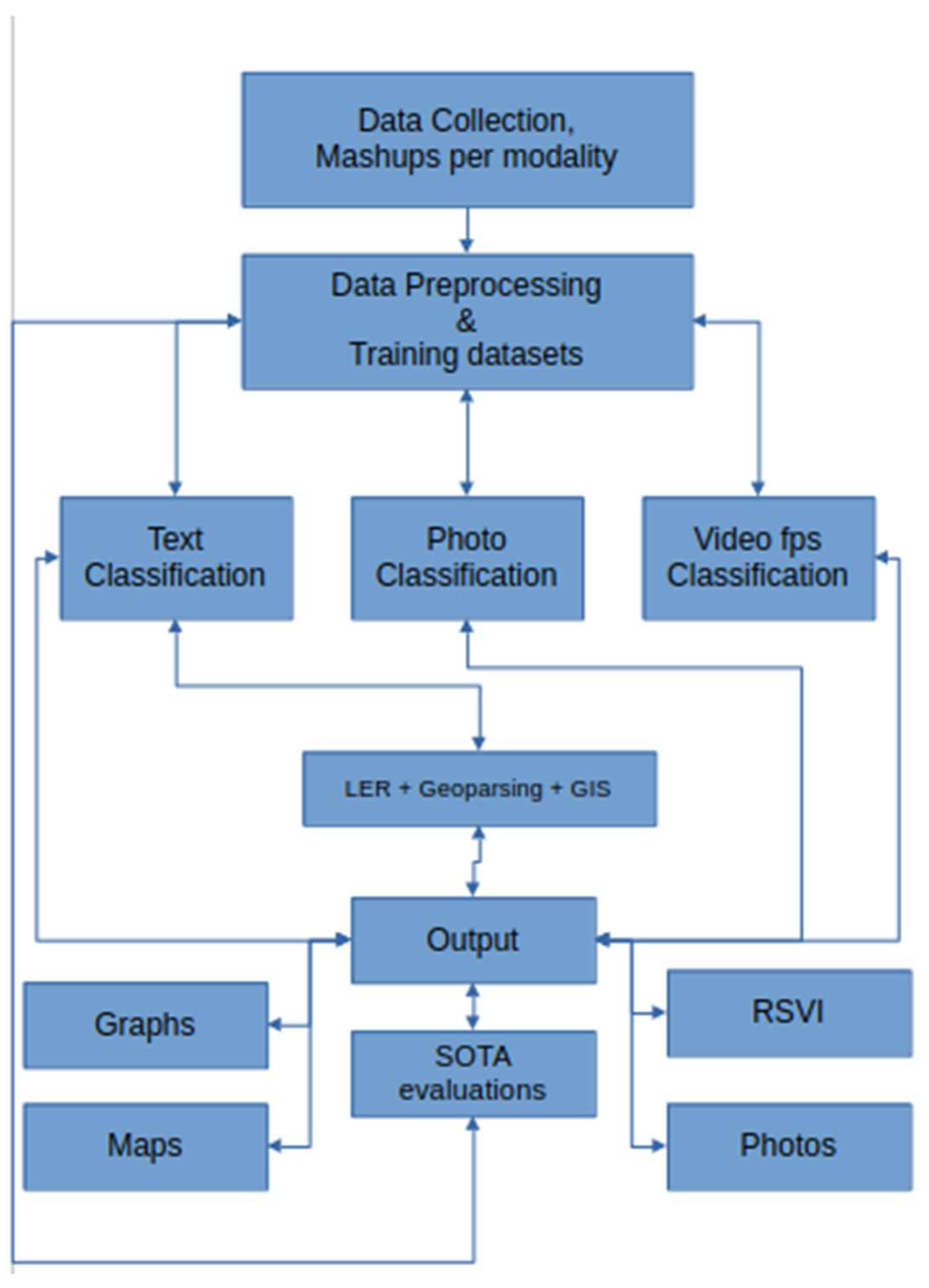
Figure 2.
Data sources and data types used.
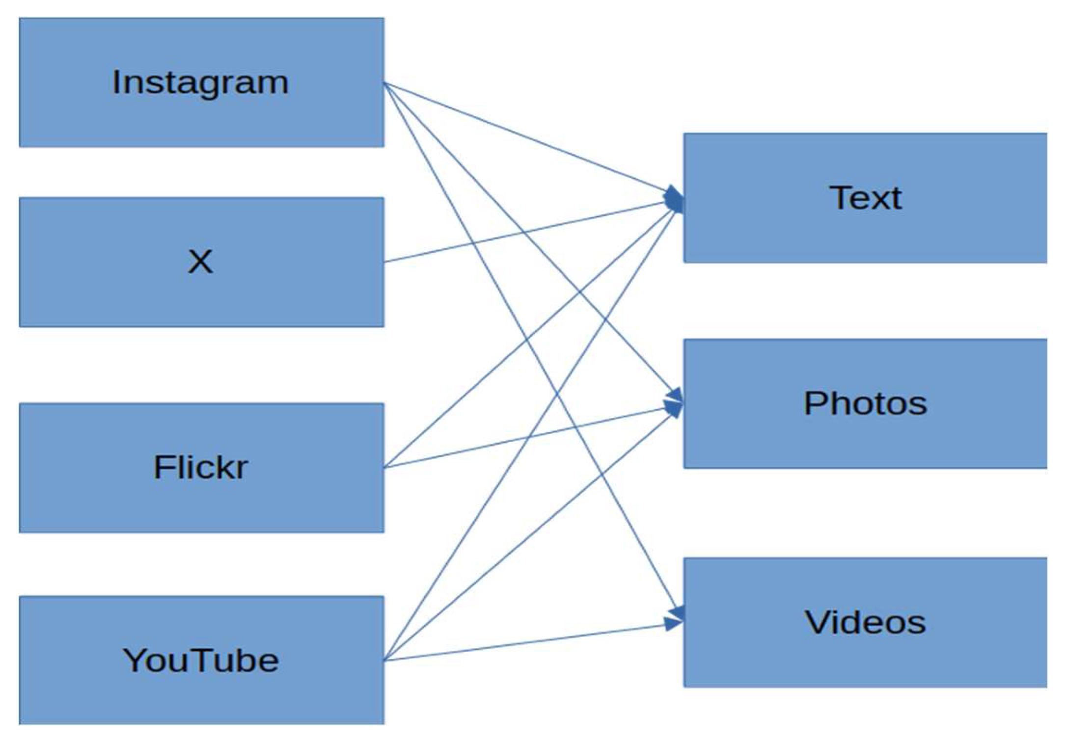
Figure 3.
Deep learning models for text classification.
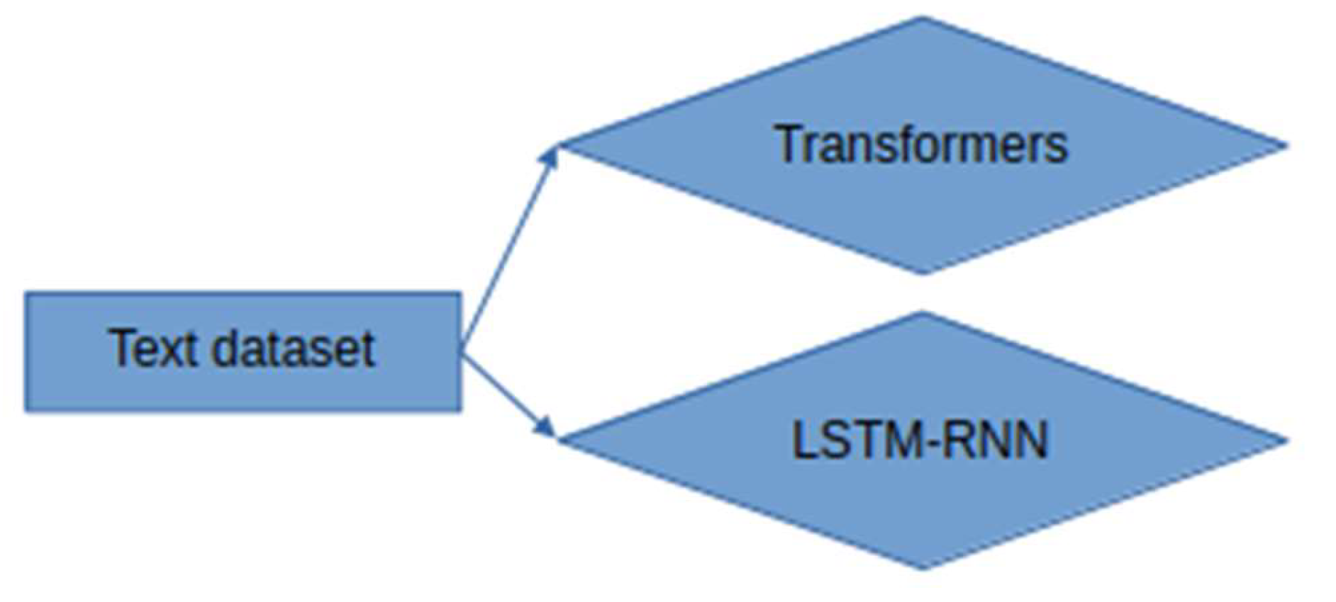
Figure 4.
Models and data participating in current ensemble approach for photo and video processing.
Figure 4.
Models and data participating in current ensemble approach for photo and video processing.
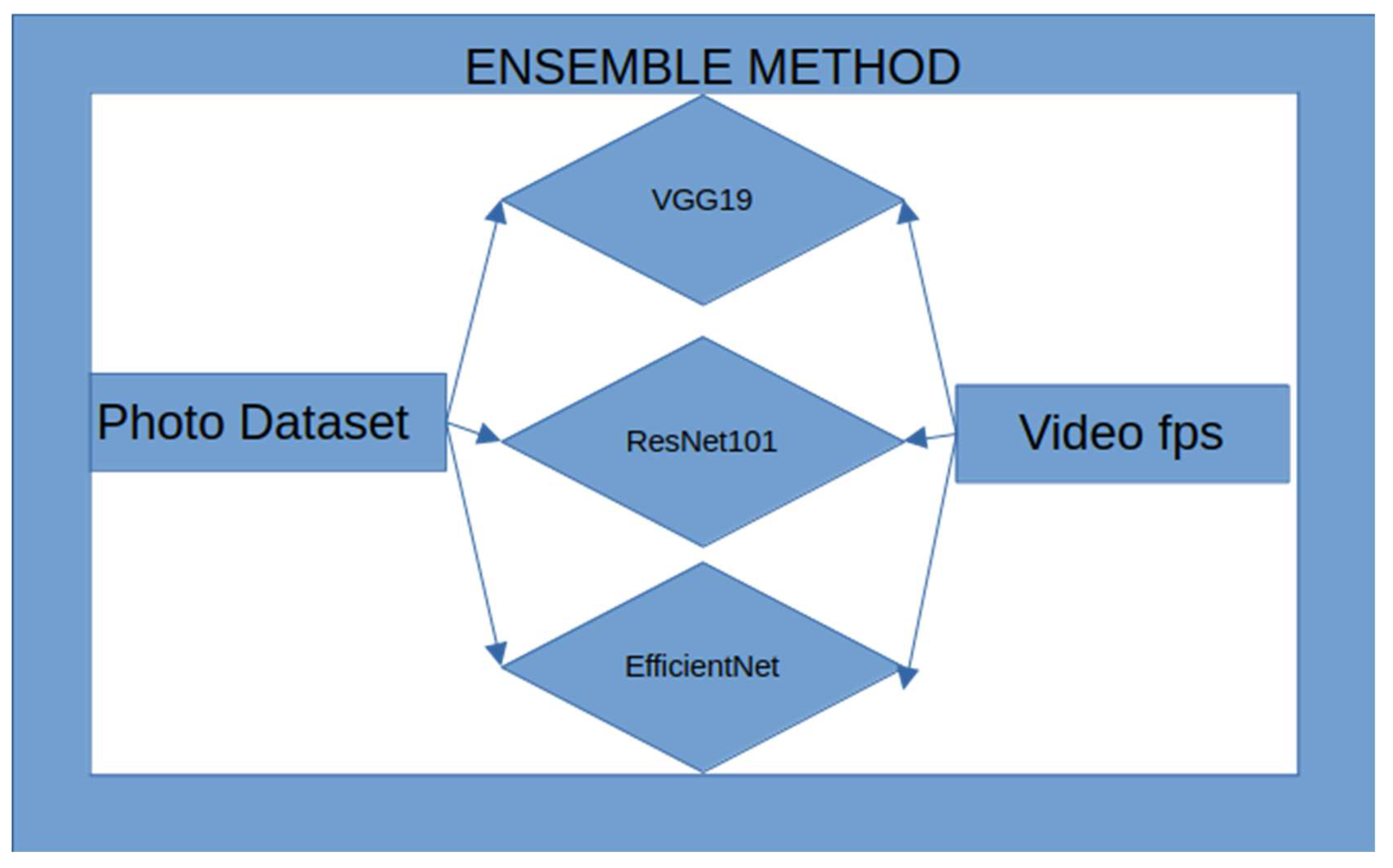
Figure 5.
Transformers, emotions, opinions etc. ~10%.
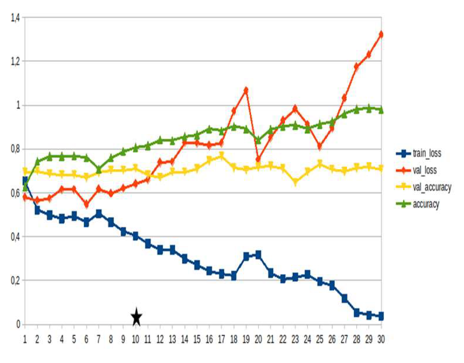
Figure 6.
Transformers, consequences ~10%.
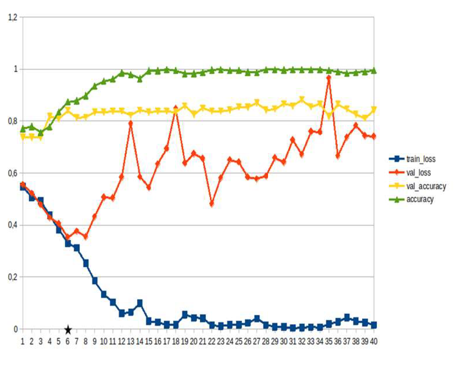
Figure 7.
Transformers, disaster management ~10%.
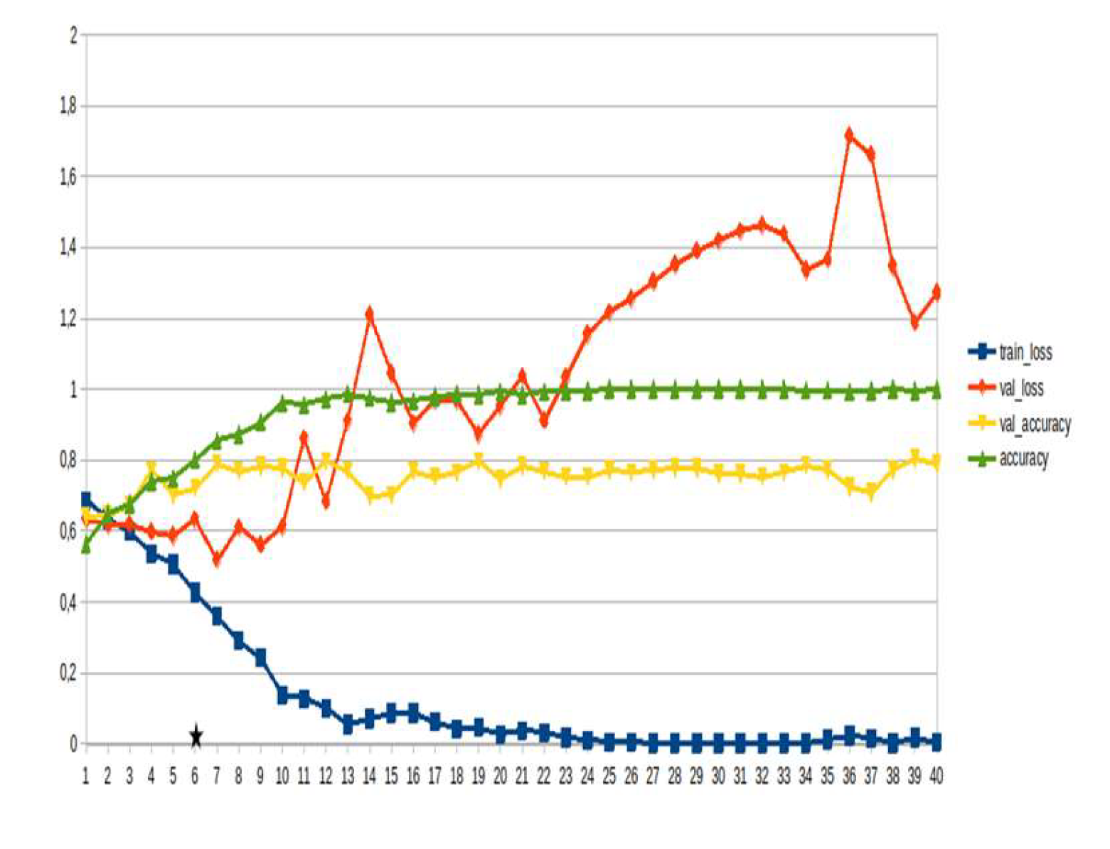
Figure 8.
Transformers, weather ~10%.
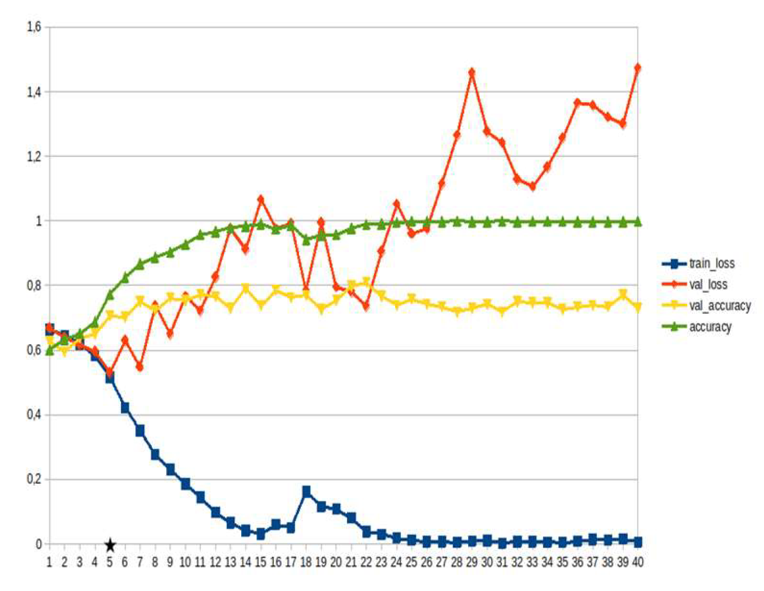
Figure 9.
Transformers, identification~10%.
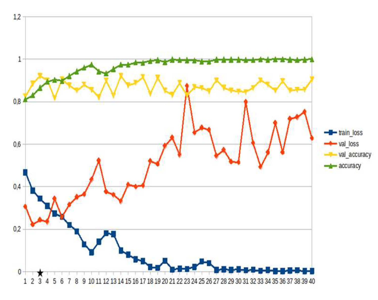
Figure 10.
Transformers, emotions, opinions etc. ~15%.
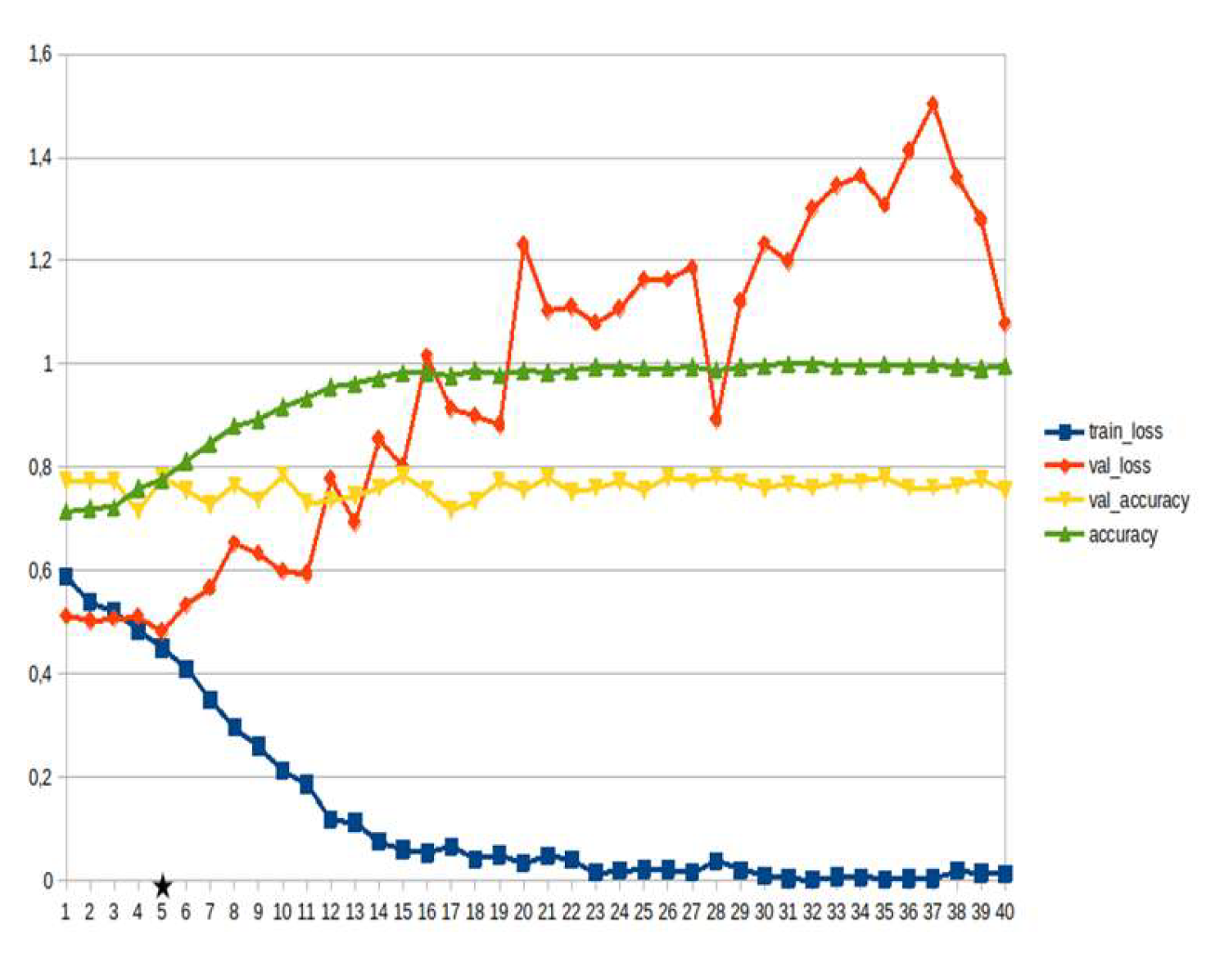
Figure 11.
Transformers, consequences ~15%.
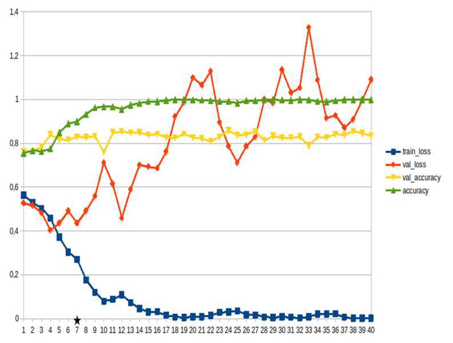
Figure 12.
Transformers, weather ~15%.
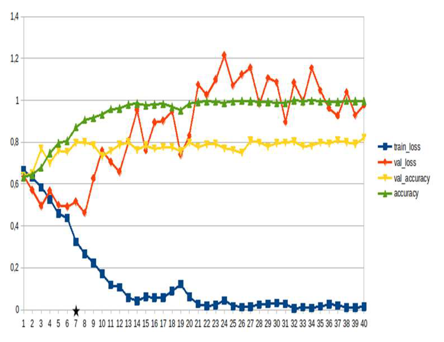
Figure 13.
Transformers, identification~15%.
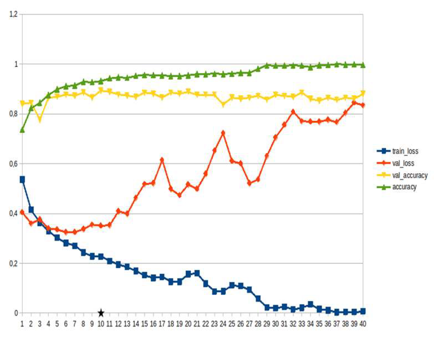
Figure 14.
Transformers, disaster management ~15%.
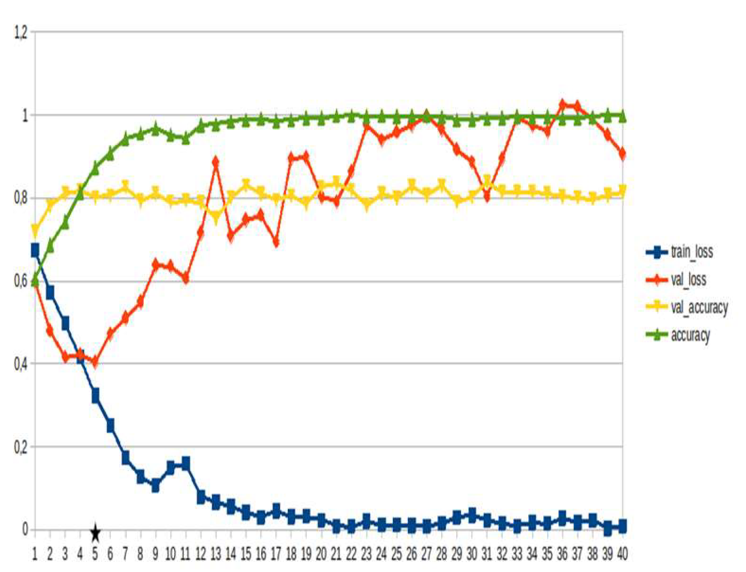
Figure 15.
LSTM, Disaster management ~10%.
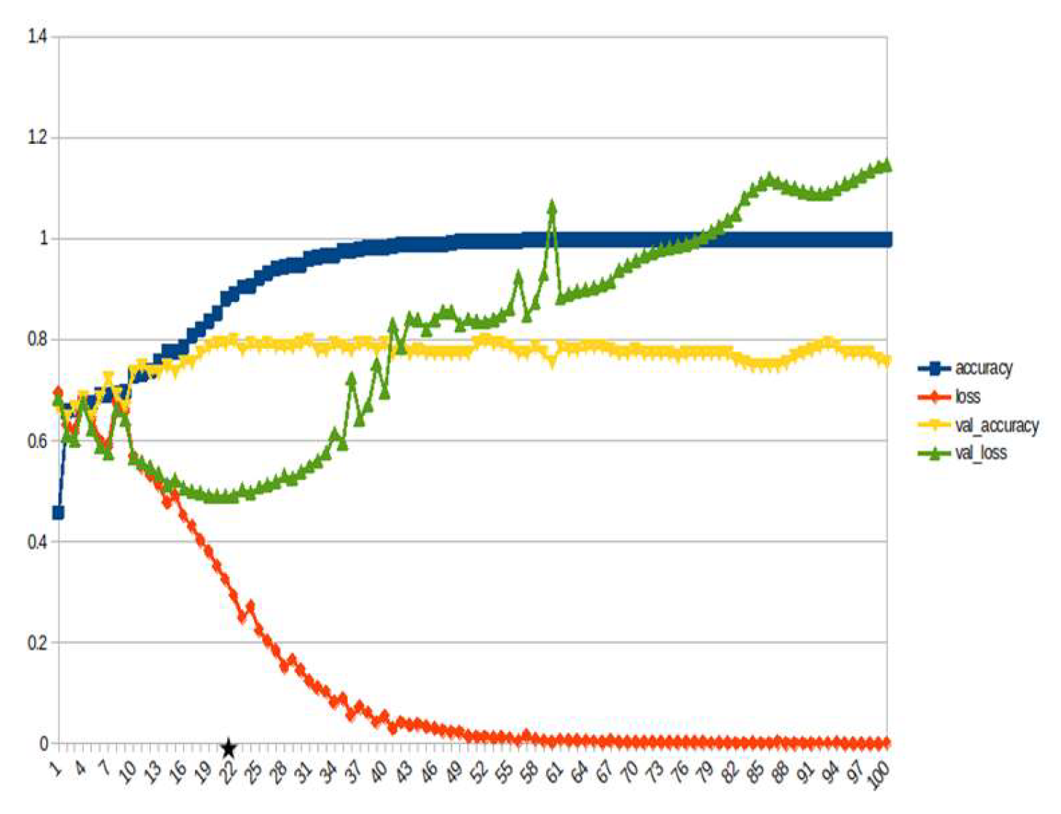
Figure 16.
LSTM, weather ~10%.
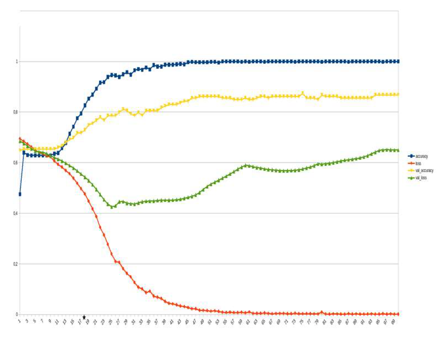
Figure 17.
LSTM, identification ~10%.
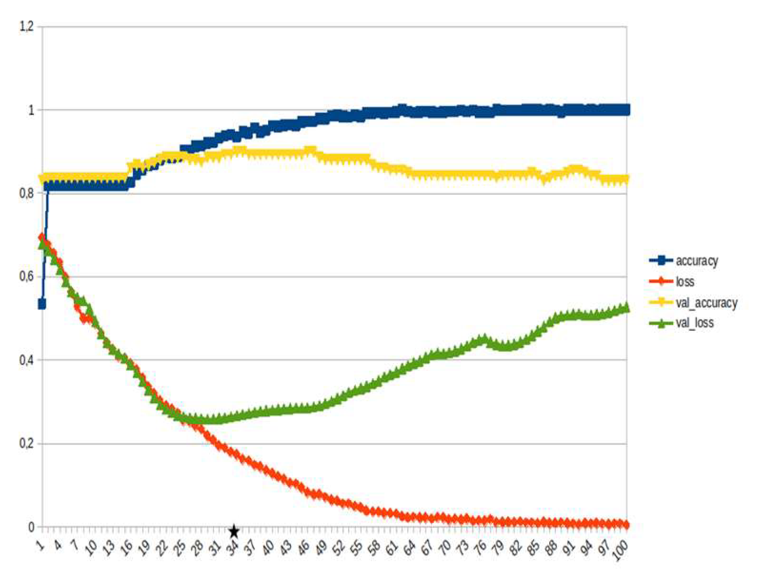
Figure 18.
LSTM, consequences ~10%.
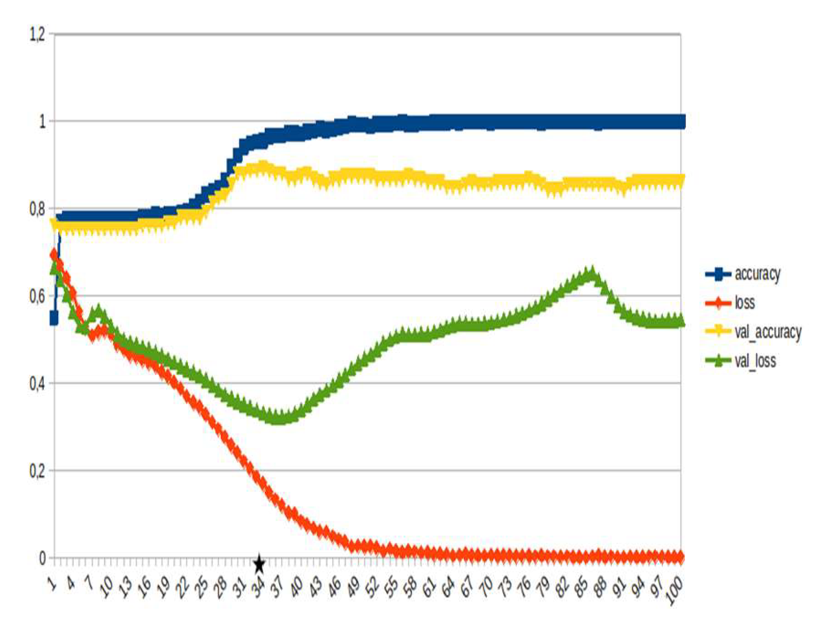
Figure 19.
LSTM, emotions, opinions , etc. ~10%.
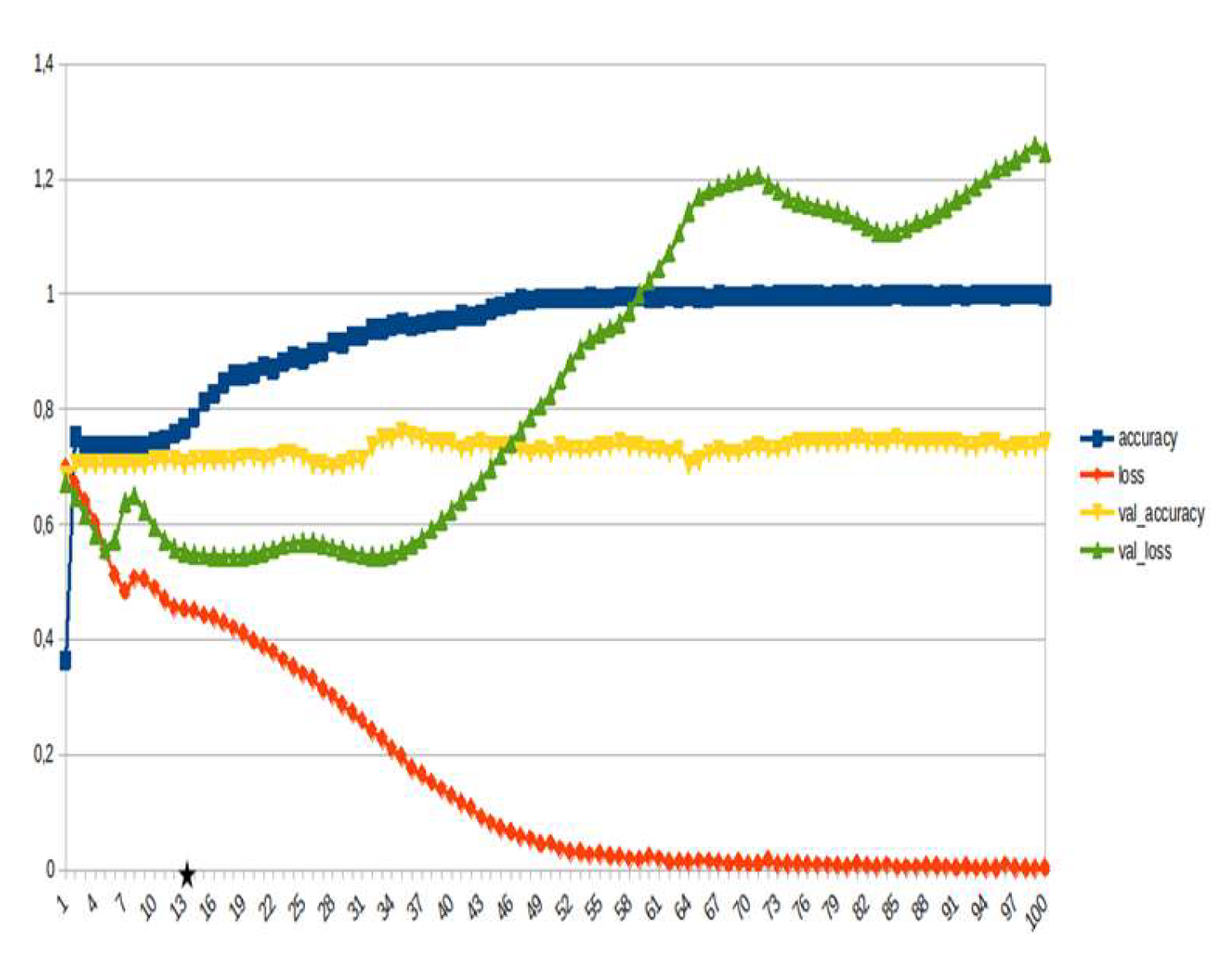
Figure 20.
LSTM, disaster management ~15%.
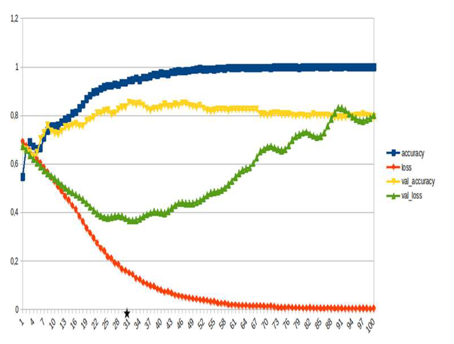
Figure 21.
LSTM, consequences ~15%.
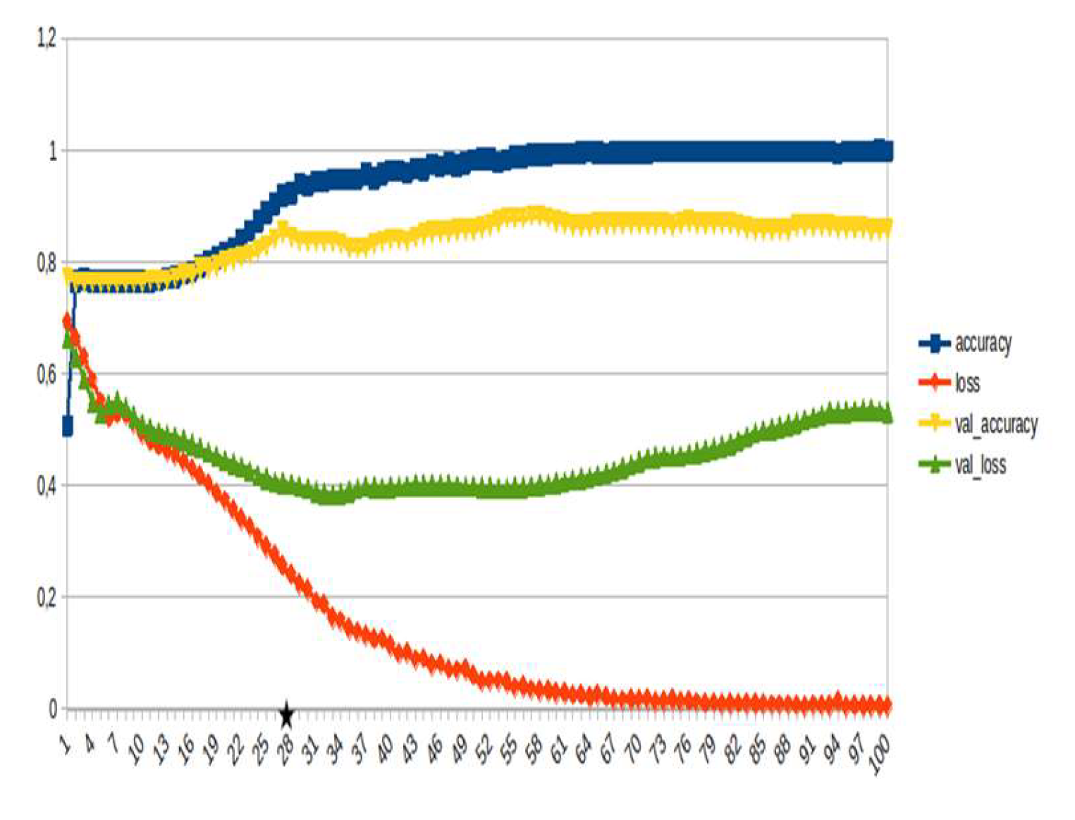
Figure 22.
LSTM, identification ~15%.
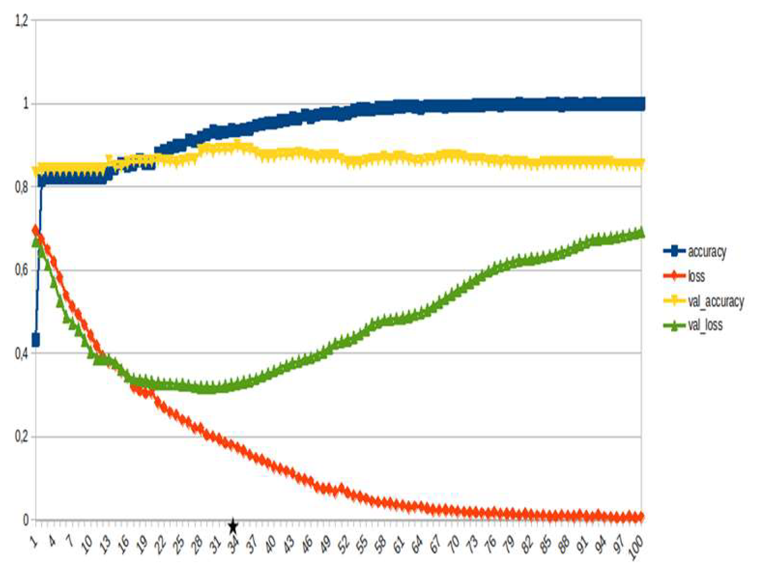
Figure 23.
LSTM, weather ~15%.
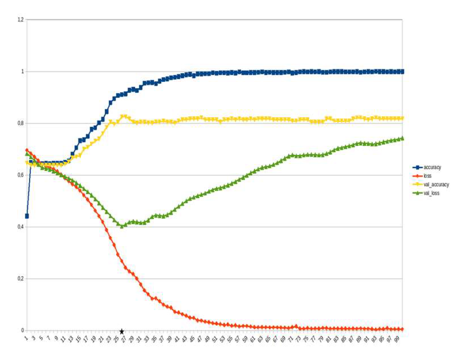
Figure 24.
LSTM, Emotions_opinions,_etc. ~15%.
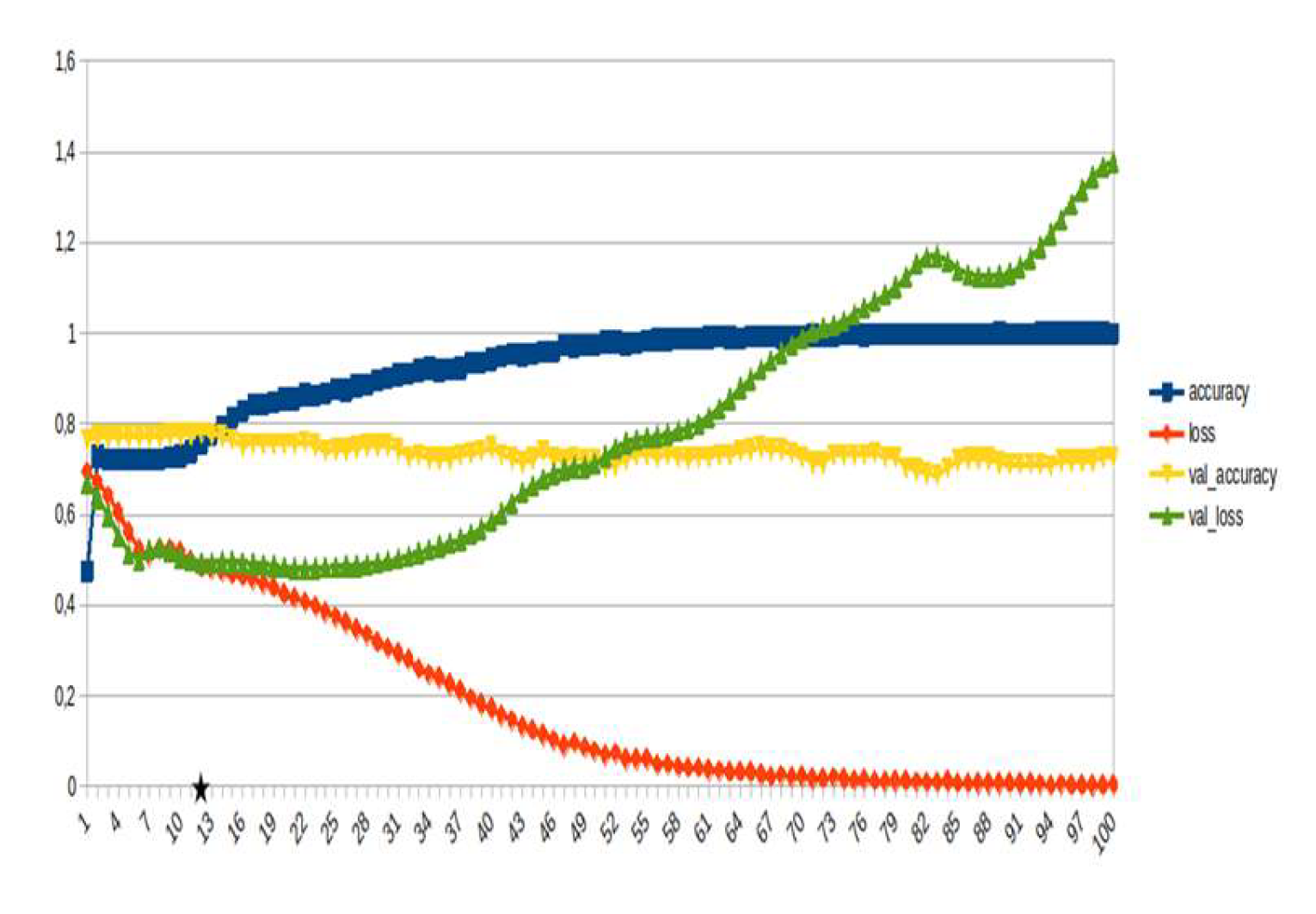
Figure 25.
Frequency of posts per class, divided into 24-hour time periods. Left: Frequency of posts per source.
Figure 25.
Frequency of posts per class, divided into 24-hour time periods. Left: Frequency of posts per source.
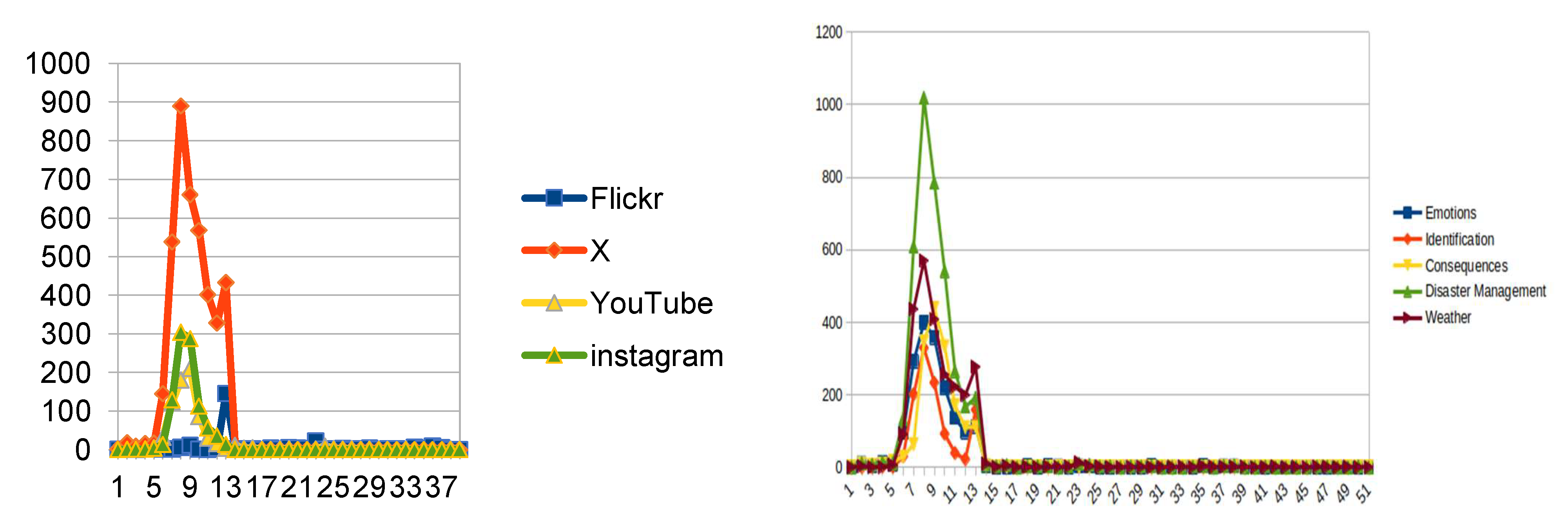
Figure 26.
Indicative photos/video frames that were successfully identified.
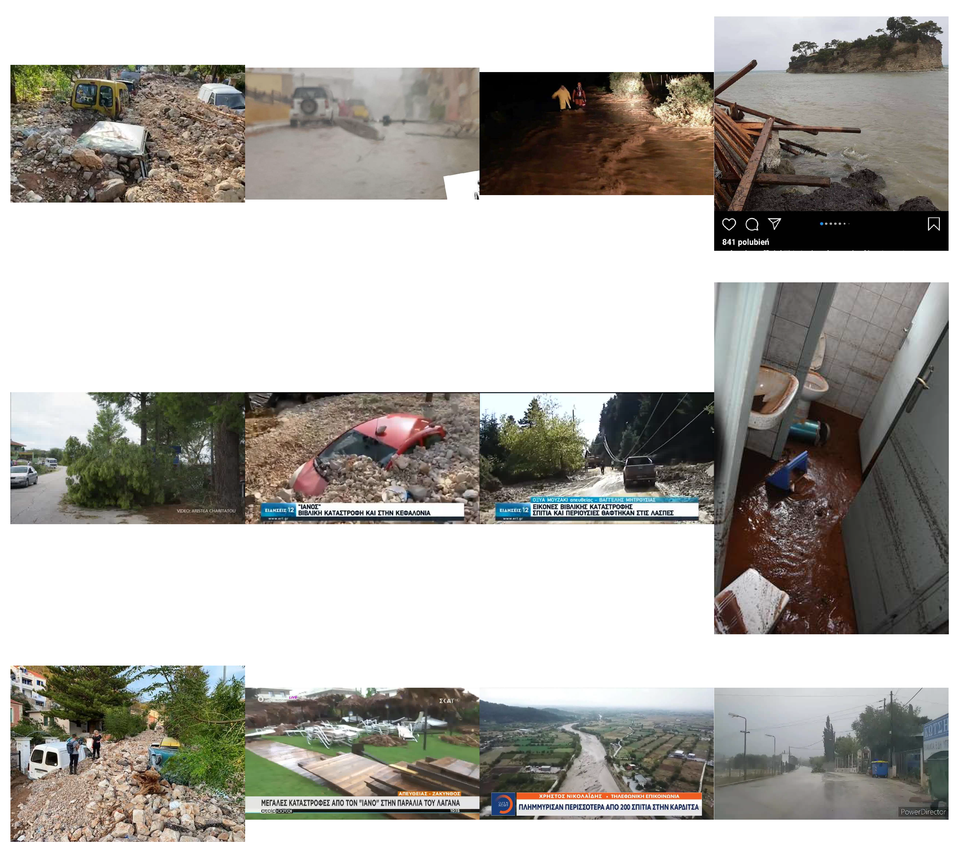
Figure 27.
Clusters of geocoded locations recognized in text strings of social media posts.
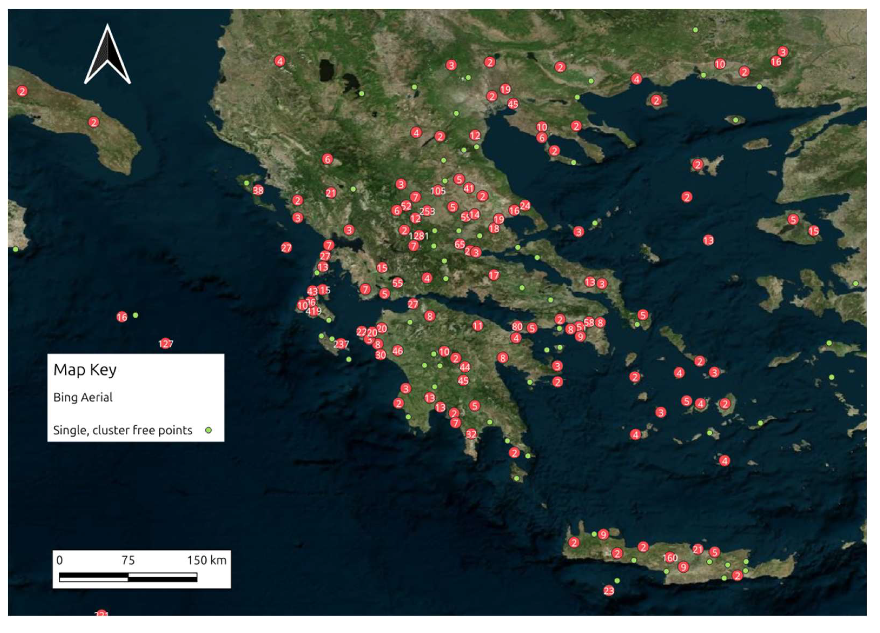
Figure 28.
Mapping locations recognized in text strings of Instagram and Flickr posts.
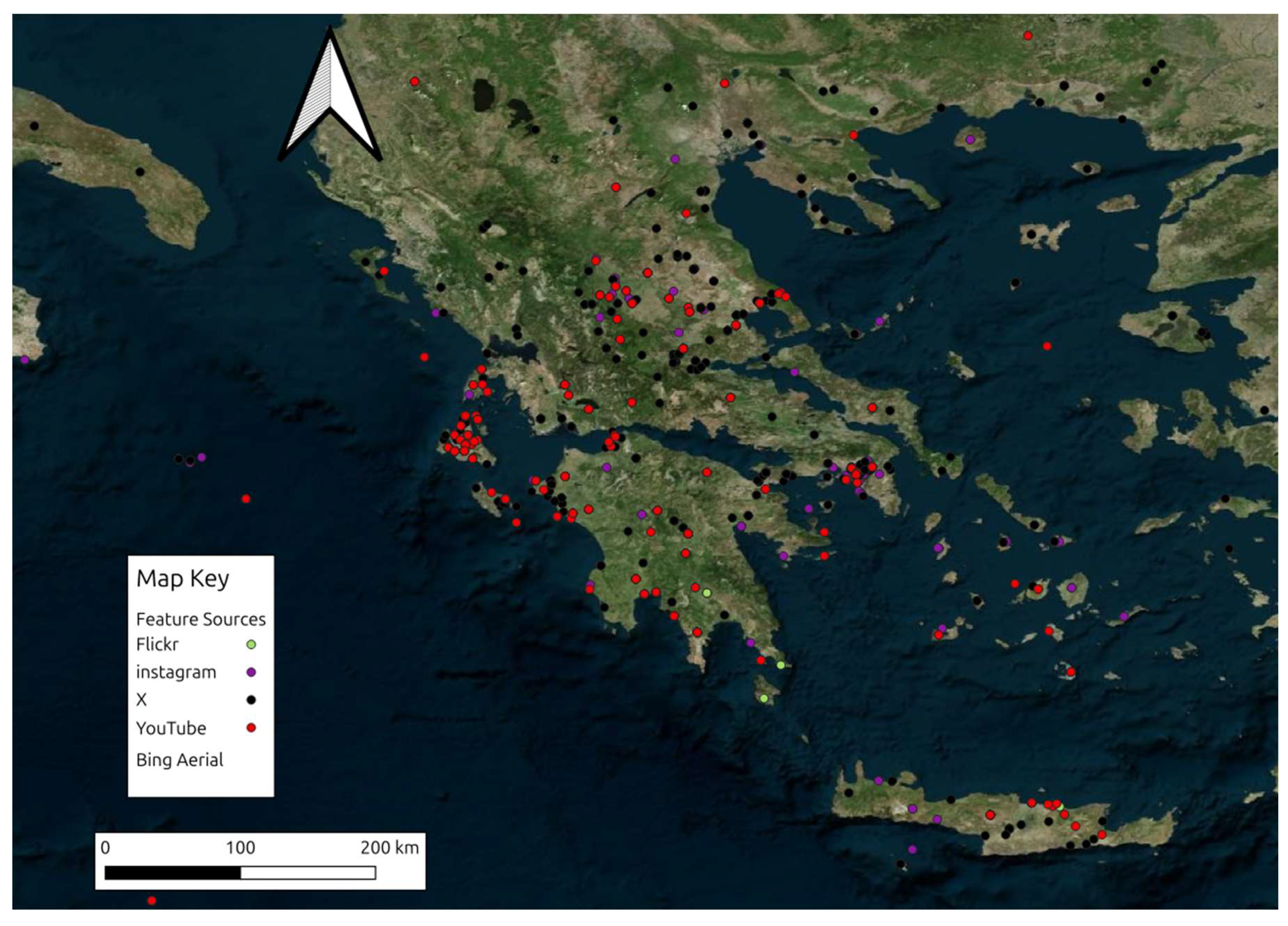
Table 1.
Classification Schema Followed for Text Classification.
| Brief Description | Class Name |
|---|---|
| Only simple identification regarding the presence of rain, strong wind etc. Not past events | Identification |
| Consequences of the Ianos: Damage, difficulties in everyday tasks, human loss, injuries, floods, electricity cut, etc. | Consequences |
| Everything regarding Tracking and Disaster Management: Information about the status, consequences, red alerts, posts that imply in situ information in photos. | Disaster Management |
| All information related to: meteo; meteo announcements; actual reports regarding weather: rain, rainy day, sunny day. Past events are not included apart from reports like: ‘rain just stopped’. | Weather |
| Emotions, opinions, comments related to Ianos only and connected effects. Statements of politicians, blame, criticism of the authorities, links like ‘read more’ and characterizations of the situation are also included. | Emotions, Opinions, Comments, etc. |
Table 2.
Parameters, LSTM–RNN.
| Value | Parameter |
|---|---|
| custom | Epoch |
| 0.2 | Drop Out |
| 100 | Hidden Layers |
| 1024 | Batch Size |
| softmax | Activation |
| 2 | Dense |
Table 3.
Parameters, Transformers.
| Value | Parameter |
|---|---|
| custom | Epoch |
| 5e-5 | Learning Rate |
| 128 | Batch Size |
Table 4.
Train Accuracy and Precision, Validation Accuracy and Precision of LSTM-RNN and Transformers in Both Training Datasets: ~10%, ~15% of the Total Volume.
Table 4.
Train Accuracy and Precision, Validation Accuracy and Precision of LSTM-RNN and Transformers in Both Training Datasets: ~10%, ~15% of the Total Volume.
| Val_Acc | Train_Acc | Model, training dataset | Val_Acc | Train_Acc | Model / training dataset |
|---|---|---|---|---|---|
| 0.92 | 0.87 | Transformers, 10% Identification | 0.9 | 0.94 | LSTM-RNN 10% Identification |
| 0.7 | 0.77 | Transformers, 10% Weather | 0.73 | 0.83 | LSTM-RNN 10% Weather |
| 0.84 | 0.87 | Transformers 10% Consequences | 0.89 | 0.96 | LSTM-RNN 10% Consequences |
| 0.72 | 0.80 | Transformers 10% Disaster Management | 0.8 | 0.89 | LSTM-RNN 10% Disaster Management |
| 0.71 | 0.81 | Transformers 10% Opinions, Comments, Emotions | 0.71 | 0.78 | LSTM-RNN 10% Opinions, Comments, Emotions |
| 0.89 | 0.93 | Transformers15% Identification | 0.9 | 0.93 | LSTM-RNN 15% Identification |
| 0.8 | 0.87 | Transformers 15% Weather | 0.83 | 0.91 | LSTM-RNN 15% Weather |
| 0.83 | 0.90 | Transformers 15% Consequences | 0.85 | 0.93 | LSTM-RNN 15% Consequences |
| 0.8 | 0.87 | Transformers Disaster Management 15% | 0.85 | 0.94 | LSTM-RNN Disaster Management 15% |
| 0.78 | 0.78 | Transformers' Opinions, Comments, Emotions 15% | 0.78 | 0.76 | LSTM-RNN Opinions, Comments, Emotions 15% |
Table 5.
SOTA Metrics of LSTM-RNN After 1 Iteration, Enriching the Training Dataset with the FPs, FΝs.
Table 5.
SOTA Metrics of LSTM-RNN After 1 Iteration, Enriching the Training Dataset with the FPs, FΝs.
| Pred. Recall | Pred. F1 | Pred. Precision | Pred. Accuracy | N = 100 |
|---|---|---|---|---|
| 0.91 | 0.81 | 0.73 | 0.94 | Identification |
| 0.92 | 0.87 | 0.83 | 0.88 | DM |
| 0.82 | 0.86 | 0.90 | 0.94 | Consequences |
| 0.91 | 0.91 | 0.91 | 0.94 | Weather |
| 0.81 | 0.76 | 0.72 | 0.89 | Opinions, comments etc. |
Table 6.
Training, Validation and Prediction Acc for all Models and Ensemble Approach.
| Pred_Acc | Validation Acc | Train Acc | N = 150 |
|---|---|---|---|
| 0.82 | 0.94 | 0.93 | VGG-19 Fine-tuned |
| 0.82 | 0.95 | 0.95 | ResNet101 fine-tuned |
| 0.69 | 0.93 | 0.94 | EfficientNet fine-tuned |
| 0.98* | 0.99* | 0.99* | Ensemble approach |
*Ensemble approach’s accuracy estimation is based on Equation 3.
Table 7.
SOTA Evaluation of Video Frames Classification: Prediction Accuracy.
| Prediction Accuracy Instagram video frames, N = 200 |
Prediction Accuracy YouTube Frames, n = 150 |
Model |
|---|---|---|
| 0.80 | 0.69 | VGG-19 fine-tuned |
| 0.81 | 0.73 | ResNet101 fine-tuned |
| 0.79 | 0.75 | EfficientNet fine-tuned |
| Actual: 0.82 | Actual: 0.77 | Ensemble approach |
Table 8.
RSVI Summary.
| Source | Mean RSVI | N of videos. |
|---|---|---|
| YouTube | 0.34 | 511 |
| 0.55 | 241 |
Disclaimer/Publisher’s Note: The statements, opinions and data contained in all publications are solely those of the individual author(s) and contributor(s) and not of MDPI and/or the editor(s). MDPI and/or the editor(s) disclaim responsibility for any injury to people or property resulting from any ideas, methods, instructions or products referred to in the content. |
© 2025 by the author. Licensee MDPI, Basel, Switzerland. This article is an open access article distributed under the terms and conditions of the Creative Commons Attribution (CC BY) license (http://creativecommons.org/licenses/by/4.0/).
Copyright: This open access article is published under a Creative Commons CC BY 4.0 license, which permit the free download, distribution, and reuse, provided that the author and preprint are cited in any reuse.


