
Submitted:
08 May 2025
Posted:
12 May 2025
You are already at the latest version
Abstract
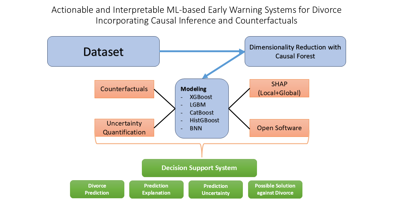
We present an interpretable machine learning framework for divorce prediction that integrates causal inference and counterfactual reasoning to generate actionable insights. Using a dataset of 170 couples (85 divorced, 85 married) assessed via the Divorce Predictors Scale (54 behavioral features), we identify 16 causally significant predictors using Double Machine Learning with Causal Forests. Notable drivers include humiliating language during arguments (ATE: +24.4%) and shared entertainment preferences (ATE: –20.8%). We train four gradient-boosting models—XGBoost, LightGBM, CatBoost, and HistGradientBoosting—and achieve high performance, with XGBoost yielding 97.9% accuracy and CatBoost achieving a ROC-AUC of 0.99. Our models outperform prior approaches, including a BERT-based Random Forest (accuracy: 81.0%) and also outperforms the state-of-theart transformer model (FT-Transformer accuracy: 97.0%), while providing greater interpretability. Our framework uniquely combines SHAP values for local and global explanations (e.g., humiliation contributing 0.11 units toward an individual’s divorce prediction), DiCE for generating diverse and plausible counterfactuals (e.g., reducing humiliation flipped the prediction to marital stability), and Bayesian Neural Networks to estimate uncertainty (±9.3% standard deviation). The entire system is accessible via an opensource Google Colab notebook, allowing users to simulate personalized interventions. This research contributes to the fields of responsible AI, computational and informational social science by demonstrating that high-accuracy prediction can be meaningfully combined with interpretability and actionability in sensitive domains. All reproducibility resources are provided via a publicly available GitHub repository
Keywords:
Interpretable AI
; Causal ML
; Diverse Counterfactual Explanations
; Human-Centered AI
; FamilyWell-being Analytics
; responsible AI
1. Introduction
Over the past few decades, divorce has become an increasingly common social phenomenon, with significant implications for individuals, families, and society at large. The once-stable institution of marriage has experienced a steady erosion, with rising divorce rates now characterizing not only Western societies but also many developing nations across various regions. According to the Organization for Economic Co-operation and Development [9], the average divorce rate across its 38 member countries is approximately 1.8 per 1,000 inhabitants annually, but in some nations, the proportion of marriages ending in divorce surpasses 40%. In the United States, nearly 45% of marriages end in divorce or permanent separation, whereas in countries like Belgium, Portugal, and Luxembourg, this number exceeds 60% [3,9]. This increase in divorce is not merely a reflection of legal liberalization or shifting cultural norms; rather, it is symptomatic of deeper transformations in gender roles, economic conditions, interpersonal expectations, and societal pressures as well. Even though divorce can sometimes be a necessary and healthy outcome, such as in cases of abuse or persistent conflict, it is more often a source of considerable personal distress associated with long-term disruption. Divorce represents one of the most emotionally taxing events of life for many individuals and is frequently associated with grief, anxiety, and a profound sense of loss [1,5]. The psychological consequences of divorce are particularly well-documented. Adults who experience divorce tend to report lower levels of life satisfaction and higher incidences of mental health disorders, including depression and anxiety [5,11]. Financial strain often follows, especially among women who may face reduced household income, increased childcare burdens, and more limited access to economic opportunities post-separation [12]. Divorce can also strain social networks, leading to a reduction in perceived and actual social support, which is a well-established buffer against psychological stress. Children also bear the effects of familial breakdown. Even though many children adjust over time, numerous studies have found that an association exists between parental divorce and negative developmental outcomes, including diminished academic performance, behavioral problems, and difficulties forming stable relationships in adulthood [2,7]. The long-term nature of these impacts highlights the urgent need for early detection and targeted support mechanisms to prevent divorce. Divorce is not inherently detrimental, but its unmitigated occurrence, particularly in high-conflict or financially insecure households, can magnify existing vulnerabilities. The social and economic costs of divorce extend beyond the individual and familial levels. Research has shown that rising divorce rates place increased pressure on legal systems, mental health services, housing markets, and welfare programs [10,13]. Governments often incur additional expenses through increased demand for public housing, social security benefits, and child welfare support. Furthermore, divorce is strongly linked to child poverty, particularly in single-parent households, which transfers the cycles of disadvantage across generations [8].
Alongside individual psychological and economic consequences, divorce can also be shaped by a broader web of sociocultural dynamics that vary across time, space, and demographic groups. In several Western societies, changing attitudes toward gender roles, individualism, and self-fulfillment have contributed to shifting expectations about marriage. As Giddens (1992) describes in his theory of the “pure relationship,” modern marriages are increasingly based on emotional intimacy and mutual satisfaction rather than economic necessity or social convention [16]. While this allows for more egalitarian and emotionally fulfilling unions, it also creates greater fragility, indicating that relationships are more likely to dissolve when emotional needs are unmet. Technological change has further complicated the landscape of romantic relationships. The rise of digital communication platforms and online dating has expanded access to potential partners while simultaneously raising expectations and reducing perceived costs of leaving an unsatisfactory relationship [19]. Moreover, social media can sometimes intensify relationship dissatisfaction by fueling comparison or miscommunication alongside suspicion [15]. These digital dynamics among younger couples often accelerate relational burnout or weaken commitment.
It is also essential to recognize that divorce is not experienced equally across cultures, genders, or socioeconomic strata. For example, in more collectivist societies like those in East Asia or the Middle East, divorce remains stigmatized and less frequent. Nevertheless, it is rising, particularly among urban, educated women who seek independence and self-actualization [17]. In contrast, in some sub-Saharan African contexts, divorce may be more fluid and culturally accepted as part of the life course, especially where bridewealth or polygamy structures influence marital dynamics [14]. Understanding divorce thus requires attention to cultural norms, legal frameworks, religious institutions, and economic opportunity structures.
Divorce rates are also highly stratified by education and income. Individuals with higher education levels tend to delay marriage, but once married, are less likely to divorce, possibly due to better communication skills, more stable employment, and greater alignment of values [18]. Conversely, lower-income individuals may face more relationship stress due to economic instability, limited access to counseling resources, and conflicting life goals. These disparities highlight the need for targeted, accessible, and context-sensitive tools that help individuals navigate relational challenges before they escalate into breakdowns.
Despite these widespread consequences, many divorces unfold after prolonged periods of silent deterioration. It extends stretches of emotional disengagement, unresolved conflict, and unmet expectations. Relationship decline is typically a gradual process during which opportunities for repair and intervention may still exist. However, couples often lack timely access to predictive or preventive tools that could alert them to these risks in meaningful, evidence-based ways.
Traditional approaches to understanding divorce have come largely from sociology, psychology, and family studies, and they offer valuable frameworks for analyzing communication breakdown, emotional regulation, attachment styles, and relational commitment [4,6]. These theories provide rich qualitative insights, but undoubtedly, their translation into scalable, data-driven systems capable of individualized assessment and intervention remains limited. Clinical models of relationship therapy, for example, are not always accessible, and self-help tools rarely incorporate rigorous evidence or personalization. At the same time, the rise of computational social science and machine learning has opened new possibilities for analyzing patterns in relational data, which provides predictive capabilities that far exceed what manual assessments can achieve. However, most machine learning models are designed solely to predict outcomes (e.g., "Will this couple divorce?") without addressing the deeper question of why that prediction is made, or what can be done to prevent it. These models are typical black-box systems, and may offer little transparency or interpretability, but almost no actionable guidance. This disconnect limits their usefulness in sensitive, emotionally charged domains like romantic relationships, where interpretability, ethical considerations, and personalization are foremost.
Therefore, there exists a critical gap between the descriptive richness of social science research and the predictive power of machine learning. Bridging this divide requires a new class of systems—ones that are not only accurate but also interpretable, causally grounded, and action-oriented. Such systems must move beyond correlation-based predictions and instead identify causal drivers of relationship breakdown. More essentially, they must be able to simulate counterfactual scenarios to provide individuals clear, data-driven answers to questions like, “What specific changes in behavior could reduce the likelihood of divorce?” Fortunately, modern data science research has produced concepts and tools that can develop systems that combine the strengths of both domains. That means, drawing from causal inference, interpretable machine learning, and counterfactual reasoning, we can move toward more responsible and impactful tools for relationship support and decision-making. In the face of a widespread and costly social challenge like divorce, such decision support systems are not merely technical achievements; rather, they are vital contributions to societal well-being.
Major contributions of our research are presented in the following bullet points:
- Introduced a Causal Forest (Double ML) approach to identify behaviorally significant drivers of divorce, moving beyond correlation to establish actionable causal relationships.
- Combined SHAP (global/local explanations) and counterfactual reasoning (DiCE) to provide transparent, personalized insights that reveals both prediction logic and preventive actions.
- Utilized Bayesian Neural Networks to quantify prediction confidence, enhancing reliability for real-world deployment.
- Released non-technical user friendly Google Colab Notebook to make the models accessible [20].
2. Related Work
Numerous studies have investigated divorce prediction as a means of addressing the rising concerns surrounding marital separation. Ameer et al. (2025) developed a two-stage predictive modeling system using a 25-item questionnaire dataset comprising responses from 300 individuals across various social backgrounds [23]. In the first stage, they applied K-Nearest Neighbors (KNN), Support Vector Machines (SVM), and Bidirectional Long Short-Term Memory (Bi-LSTM) models. In the second stage, they used Recursive Feature Elimination (RFE) to identify the most influential features, then retrained the models—along with an additional Apriori algorithm—on the reduced dataset. Among all methods, KNN yielded the best performance with an F1-score of 0.932, outperforming models from the initial phase.
Dina et al. (2024) employed IndoBERT and TF-IDF for divorce prediction using historical court case records from Surabaya’s Religious Court [24]. To handle class imbalance, they applied oversampling techniques and optimized model parameters using grid search. Among the models tested, the Random Forest classifier delivered the best results, achieving a precision of 0.82 and accuracy of 0.81.
Tabrizi et al. (2024) utilized socioeconomic data sourced from Iranian Judiciary Courts covering the period from 2011 to 2018 [25]. Their models were validated through a rigorous 10-fold cross-validation process. Random Forest and Neural Networks demonstrated the strongest performance, with AUC scores of 0.981 and 0.979, respectively. Key features influencing divorce prediction included unemployment rates and urbanization levels, highlighting the role of broader economic factors in marital outcomes.
Moumen et al. (2024) explored the use of machine learning to evaluate the effectiveness of the Divorce Predictors Scale (DPS) in the Hail region of Saudi Arabia [26]. Rooted in Gottman’s couples therapy framework, the DPS was administered alongside a personal information form to collect demographic data from 148 participants (116 married, 32 divorced). Using Artificial Neural Networks, Naïve Bayes, and Random Forest models, the study found that the RF classifier achieved the highest accuracy (91.66%). Feature selection was performed via correlation analysis, and the study concluded that the DPS is a reliable tool for supporting family counseling and intervention planning.
Sahle et al. (2024) [31] investigates a hybrid approach combining ensemble learning techniques—AdaBoost, Gradient Boosting, Bagging, Stacking, XGBoost, and Random Forest—with nature-inspired optimization algorithms, namely Jaya and Whale Optimization Algorithm (WOA). Model performance was evaluated using both train-test splits and k-fold cross-validation by employing key metrics such as accuracy, precision, recall, F1-score, and the Area Under the Receiver Operating Characteristic Curve (AUC-ROC). Among the ensemble models, AdaBoost emerged as the top performer, achieving accuracies of 97% and 96% with Jaya and WOA-based hyperparameter optimization, respectively. The study supports the development of socially responsible and sustainable technological solutions by leveraging artificial intelligence for divorce prediction.
Satu et al. (2024) [27] proposed an explainable AI (XAI)-based model to identify key factors that distinguish divorced individuals from happily married couples, based on the output of the best-performing classifier. They used a divorce prediction dataset from the University of California Irvine (UCI) Machine Learning Repository, which was preprocessed and analyzed using various classification algorithms. Among these, the Support Vector Machine (SVM) achieved the highest classification accuracy of 98.23%. To enhance interpretability, the authors applied Shapley Additive Explanations (SHAP), a widely used XAI method, to analyze the SVM model and determine which features most influenced the predictions.
Ventura-León et al. (2024) conducted a study to predict the end of romantic relationships among 429 youths using a SMOTE-balanced dataset [28]. They applied Logistic Regression, Gradient Boosting, Support Vector Machines, and Random Forest, using stratified random sampling to split the data into training (80%) and validation (20%) sets. Model performance was evaluated via 10-fold cross-validation across standard metrics. To improve interpretability, SHAP values were used to explain feature contributions. The authors also performed hyperparameter tuning and additional analyses to deepen their understanding of the predictors of relationship dissolution. Among all models, Random Forest achieved the highest performance across the evaluation metrics.
Kumar et al. (2023) utilized a dataset from the UCI Machine Learning Repository that contains relationship questionnaire responses from couples [29]. After preprocessing, the authors ranked features using Information Gain, OneR, Gain Ratio, and ReliefF. They then implemented several classifiers, including Logistic Regression, Naïve Bayes, Stochastic Gradient Descent (SGD), Decision Tree, Random Forest, and Multilayer Perceptron (MLP). Models were evaluated using the full feature set and top-ranked subsets (6 and 7 features), across multiple data splits (50:50, 66:34, 80:20) and 10-fold cross-validation. Remarkably, Decision Tree, Random Forest, and MLP classifiers reached 100% accuracy using the top 7 features, highlighting the high predictive power of key relationship indicators.
Ahsan et al. (2023) applied six machine learning models—Logistic Regression, Linear Discriminant Analysis, K-Nearest Neighbors, CART, Gaussian Naïve Bayes, and SVM—to predict divorce outcomes [30]. SVM, KNN, and LDA achieved the highest accuracy, up to 98.57%. A significant contribution of this work is the use of Local Interpretable Model-Agnostic Explanations (LIME), which provided individualized, transparent explanations of model predictions. Additionally, the authors developed an interactive tool that leverages the ten most influential features, enabling users to assess their relationship status and explore potential risks of divorce through an intuitive interface.
Despite notable progress in divorce prediction using machine learning, ranging from traditional classifiers to deep learning and oversampling techniques, existing studies often prioritize accuracy over interpretability, limiting their practical utility for decision-makers like counselors and therapists. Moreover, few works have integrated causal inference or counterfactual reasoning to move beyond correlation and deliver actionable recommendations. This gap highlights an opportunity for the computing and information science community to develop models that are not only predictive but also explainable, fair, and intervention-ready. To address this, our research aims to build an interpretable machine learning framework for divorce prediction that synthesizes causal analysis, counterfactual reasoning, and uncertainty estimation to enhance explainable artificial intelligence (XAI) in socially sensitive domains. Our objective is twofold: (1) to identify causally relevant behavioral factors that influence marital outcomes using Double Machine Learning, and (2) to provide personalized, interpretable, and uncertainty-aware divorce predictions using a combination of gradient-boosted models, SHAP values, counterfactual explanations (DiCE), and Bayesian inference. The methodology section below details this multi-pronged approach.
3. Methodology
This section provides a detailed overview on how the research is conducted. All implementation codes and workflows are publicly available in our GitHub repository [21].
3.1. Dataset Information
For model development, we utilized a publicly available dataset from Kaggle [22]. The dataset comprises responses from 170 couples-either divorced or happily married—collected through face-to-face interviews. Each record includes 54 features based on the Divorce Predictors Scale (DPS), derived from principles of Gottman couples therapy. Responses were recorded on a five-point Likert scale: 0 = Never, 1 = Seldom, 2 = Averagely, 3 = Frequently, and 4 = Always. The dataset consists of 170 observations and 55 variables, including the target variable (“Divorce”). It is clean, with no missing values or duplicated entries. Given the uniform Likert-scale structure, homogeneity of variance across features is preserved. Additionally, as depicted in Figure 1, the dataset exhibits a balanced class distribution. For full transparency, the complete list of 54 features, along with their corresponding scale definitions, is provided in the Supplementary Materials section.
3.2. Causal Feature Selection
In machine learning, it is a widely accepted rule of thumb that the number of training instances should be at least ten times greater than the number of input features. Given that our dataset contains only 170 observations and 54 features, dimensionality reduction was essential to avoid overfitting and to improve model generalizability. Traditional feature reduction methods such as Principal Component Analysis (PCA), Recursive Feature Elimination (RFE), Genetic Algorithm (GA), and Particle Swarm Optimization (PSO) are commonly used, but they do not consider causal relationships among features. In particular, GA and PSO rely heavily on randomization, which limits their interpretability and causal rigor.
To address this limitation, we employed a Causal Forest–based approach under the Double Machine Learning (DML) framework to identify the top 16 features with a causal impact on the target variable, “Divorce.” This selection aligns with the 10:1 instance-to-feature ratio guideline (i.e., 16 × 10 = 160), making our dataset appropriate for training supervised models.
Our causal inference pipeline involved the following steps: First, each of the 54 features was predicted using a Random Forest classifier to identify its most influential covariates. Features that cumulatively accounted for 80% of the total importance scores were treated as potential confounders. Next, each feature was considered as a potential treatment variable, and its Average Treatment Effect (ATE) on the binary outcome “Divorce” was estimated using the DML procedure. Specifically, a two-stage machine learning process was applied: in the first stage, both the treatment and outcome were regressed on the identified confounders using Random Forests to eliminate spurious associations. In the second stage, residuals from these regressions were used to estimate the ATE through orthogonalization, thereby reducing the risk of overfitting and enhancing robustness to high-dimensional confounding.
The resulting ATEs were ranked, and the 16 features with the largest and statistically meaningful causal influence on divorce () were selected for downstream modeling. These features were not only informative but also causally relevant, offering stronger explanatory power than features selected through traditional statistical or randomized techniques. This approach enhances both the predictive performance and interpretability of subsequent machine learning models.
|
Algorithm 1 Causality-Aware Dimensionality Reduction using Double Machine Learning (DML)
|
|
Input: Dataset D with n samples and d features ; binary target variable Y (Divorce)
Output: Top-k causally relevant features , where
|
The Average Treatment Effect (ATE) quantifies the expected change in the outcome variable. In our case, the probability of divorce, resulting from a unit increase in a particular feature, while holding all identified confounders constant.
Formally, the ATE for a feature is defined as:
where Y is the binary outcome variable (Divorce), and denotes an intervention in the causal graph, following Pearl’s do-calculus framework. This formulation captures the causal impact of an external change in on the probability of divorce.
3.3. Model Selection
We selected four state-of-the-art gradient boosting models and one neural network architecture to model the divorce prediction dataset. The gradient boosting–based ensemble models include Extreme Gradient Boosting (XGBoost), Light Gradient Boosting Machine (LGBM), Categorical Boosting (CatBoost), and the Histogram-based Gradient Boosting (HistGradientBoosting) classifier. These models are particularly optimized for structured tabular datasets with moderate dimensionality and limited sample size. Unlike deep learning models, which typically require large volumes of data and continuous features, gradient boosting decision trees are well-suited for handling ordinal, categorical, and numerical data formats.
Divorce prediction involves complex and subtle patterns stemming from behavioral, emotional, and interpersonal variables such as communication and emotional expression. Tree-based models are naturally adept at capturing such nonlinear relationships and feature interactions, making them particularly well-suited for modeling relational dynamics. Moreover, given the small sample size (170 instances), overfitting is a critical concern. All four ensemble models incorporate built-in regularization mechanisms—such as L1/L2 penalties, shrinkage, and early stopping—that improve generalization and model robustness.
Another advantage of these models is their compatibility with post-hoc explainability tools such as SHAP (SHapley Additive exPlanations). SHAP enables both local (individual-level) and global (dataset-level) interpretability, which is crucial for sensitive applications like relationship assessment. We integrated SHAP-based explanations to enhance transparency and trust in the predictions.
Hyperparameters for all ensemble models were optimized using Bayesian Optimization to balance predictive performance and complexity. In addition to these models, we employed a Monte Carlo (MC) dropout–based Bayesian Neural Network (BNN), primarily for uncertainty quantification. While the BNN is capable of performing classification tasks, its core utility lies in estimating prediction uncertainty—an aspect that traditional ensemble methods do not inherently support. This model can be particularly valuable to end-users interested not only in prediction outcomes but also in how confident the model is in its decisions. By combining explainable gradient boosting classifiers with a probabilistic neural approach, we aim to develop a robust and interpretable early warning system for relationship dissolution.
Before starting the modeling process, we split our dataset into an 80:20 ratio for training and testing. We used stratify=y during the split to ensure that both subsets maintain the same class distribution as the original dataset. This is important in binary classification tasks like predicting Divorce vs. Non-Divorce. It assists in preventing any class imbalance in the test set that could bias model evaluation or lead to misleading performance metrics. Basic description of the chosen models is given below.
3.3.1. XGBoost: eXtreme Gradient Boosting
XGBoost is a scalable and regularized implementation of gradient boosting decision trees designed for performance and model generalization. It constructs an ensemble of additive weak learners (usually decision trees) in a stage-wise manner to minimize a differentiable loss function.
The prediction for an instance is made by summing over K decision trees:
where is an individual regression tree, and is the space of all possible trees.
The overall objective function to minimize at iteration t is defined as:
where l is a convex differentiable loss function (e.g., logistic loss for classification), and is a regularization term that penalizes model complexity to avoid overfitting.
The regularization function is given by:
Here, T is the number of leaves in the tree, is the score on leaf j, and , are regularization parameters controlling tree complexity and weight shrinkage.
To add a new function at iteration t, a second-order Taylor expansion of the loss is used:
where:
- is the first-order gradient
- is the second-order gradient (Hessian)
This use of both first and second derivatives allows XGBoost to efficiently and accurately optimize arbitrary loss functions, providing improved convergence and model performance.
3.3.2. LightGBM: Light Gradient Boosting Machine
LightGBM is another highly efficient gradient boosting framework developed by Microsoft, designed for speed and scalability as an alternative of XGBoost. It introduces two major innovations over traditional gradient boosting frameworks. First of all, Gradient-based One-Side Sampling (GOSS), and secondly, Exclusive Feature Bundling (EFB), which enable faster training on large and sparse datasets while maintaining high accuracy.
Similar to other gradient boosting methods, the model builds an ensemble of decision trees. The prediction for an instance is given by:
where each is a regression tree, and is the space of possible trees.
At each iteration, LightGBM seeks to minimize the regularized objective function:
Using a second-order Taylor expansion around , the objective becomes:
where:
- is the first-order gradient
- is the second-order gradient (Hessian)
Gradient-based One-Side Sampling (GOSS) retains instances with large gradients (high training error) and randomly samples those with small gradients, ensuring that the model focuses on hard-to-fit examples without losing distributional information.
Exclusive Feature Bundling (EFB) reduces the number of features by bundling mutually exclusive features into a single feature, that drastically reduces dimensionality and memory usage. Furthermore, LightGBM uses leaf-wise tree growth (as opposed to level-wise in traditional GBMs), choosing the leaf with the maximum delta loss to split. While this can lead to deeper trees, it significantly improves accuracy:
Due to these optimizations, LightGBM provides both higher efficiency and superior performance on structured datasets, making it especially effective for tabular data like divorce prediction.
3.3.3. CatBoost: Categorical Boosting
CatBoost is a gradient boosting algorithm developed by Yandex. It is specifically optimized for handling categorical features and reducing overfitting, and is based on oblivious decision trees (symmetric trees). The model introduces two key innovations: ordered boosting and efficient categorical encoding.
As with other boosting models, CatBoost builds an ensemble of additive regression trees to minimize a loss function. The prediction for an instance is expressed as:
where each is a decision tree, and is the space of all symmetric trees.
At each boosting step, the model minimizes the following regularized objective:
Using second-order Taylor approximation:
where:
- is the gradient
- is the Hessian
CatBoost’s strength lies in its treatment of categorical variables. Instead of traditional one-hot encoding, CatBoost uses target statistics in a way that prevents target leakage by applying an ordered encoding scheme. That is, for each example, the categorical feature is encoded using the statistics derived only from prior samples in a random permutation of the dataset. CatBoost also introduces ordered boosting, a novel variant of gradient boosting that eliminates the prediction shift problem commonly caused by target leakage in standard boosting algorithms. In ordered boosting, for each sample, separate models are trained that only use samples seen earlier in the permutation:
where denotes predictions from models trained without using the i-th sample or any that follow it.
Finally, CatBoost uses symmetric (oblivious) trees, which grow all branches of the tree to the same depth with the same splitting criteria. It helps the model for fast inference and hardware optimization. Due to these innovations, CatBoost excels at handling datasets with high-cardinality categorical features and small sample sizes that turns it ideal for structured problems like divorce prediction where input features are ordinal or categorical in nature.
3.3.4. HistGradientBoosting: Histogram-Based Gradient Boosting
HistGradientBoosting is another gradient boosting algorithm designed for efficient handling of large datasets by using histogram binning to approximate the gradient and Hessian computations. This feature makes it faster and more memory-efficient than traditional gradient boosting methods. It is based on decision trees and utilizes histogram-based discretization for continuous features, which enables faster training and lower memory usage. As with other boosting models, HistGradientBoosting builds an ensemble of additive regression trees to minimize a loss function. The prediction for an instance is expressed as:
where each is a decision tree, and is the space of all trees.
At each boosting step, the model minimizes the following regularized objective:
Using second-order Taylor approximation:
where:
- is the gradient
- is the Hessian
HistGradientBoosting’s strength lies in its histogram-based binning technique that discretizes continuous features into bins and approximates the gradient and Hessian over the bins. It significantly improves training speed and reducing memory consumption. This is especially useful for large datasets with many features. Also, HistGradientBoosting uses histogram-based decision trees that discretize continuous features into histograms for more efficient computation. This approach speeds up the training process while maintaining the predictive power of traditional decision trees.
3.3.5. Bayesian Neural Network (BNN) with MC Dropout
Bayesian Neural Networks (BNNs) provide a way to model uncertainty in neural networks by approximating the posterior distribution over the model’s weights. An effective approach to achieve this is to use Monte Carlo (MC) Dropout that allows the network to perform Bayesian inference during the forward pass by enabling dropout during both training and inference.
In our implementation, a simple feed-forward neural network is built using Keras, with the key modification being the inclusion of dropout layers during both training and testing. The model architecture consists of a hidden layer with 16 neurons and a ReLU activation function, followed by a dropout layer with a rate of 0.2, and a final output layer with a sigmoid activation function for binary classification.
The model is compiled using the Adam optimizer with a learning rate of 0.01 and binary cross-entropy as the loss function. After training the model for 500 epochs, the next step is to perform MC Dropout during inference. This is achieved by running multiple forward passes (in our case, 1000) with the dropout active to obtain multiple predictions for each test sample.
The model prediction is expressed as:
where represents the individual predictions obtained from the j-th dropout-enabled forward pass, and N is the total number of samples (in this case, 1000).
The uncertainty of the predictions is quantified using the standard deviation of the MC samples, in order to provide insight into the model’s confidence in its predictions. The mean prediction is then thresholded at 0.5 to convert the continuous output into binary predictions (Divorce or Non-Divorce). Such approach effectively captures model uncertainty.
We presented the 95% Confidence Interval of the performance metrics to quantify the uncertainties in ensemble models. These metrics include accuracy, precision, recall, F1 score, and AUC score. While the confidence interval is not as robust as BNN’s uncertainty quantification, they still provide valuable insights on prediction uncertainty.
3.3.6. Model Interpretability
Given that machine learning models, including the four ensemble models used in this study, are often considered "black-box" models, their predictions are not always easy to interpret. While these models deliver predictions, understanding why these predictions are made remains a challenge. As noted in the literature review, much of the existing research focuses solely on predictive accuracy, without addressing the need for interpretability. To overcome this limitation, we incorporated SHAP (SHapley Additive exPlanations) into our analysis, providing both local and global interpretability.
SHAP’s local interpretability explains why a specific prediction was made for an individual instance, offering insight into the model’s decision process. In contrast, global interpretability aggregates local explanations across all instances, revealing which features consistently influence the model’s predictions. By examining these global explanations, we can determine which features are more likely to push a prediction toward "Divorce" (1) versus "Non-Divorce" (0).
In addition to SHAP, we also utilized DiCE (Diverse Counterfactual Explanations) to generate actionable insights. While SHAP focuses on explaining the reasons behind a given prediction, DiCE examines how small changes in input features could lead to a different outcome. Specifically, DiCE provides a set of diverse counterfactual examples, answering the question: "What minimal changes in the input variables would have resulted in a prediction of Non-Divorce (0) instead of Divorce (1), or vice versa?" This allows for deeper insights into potential interventions or factors influencing the outcome.
DiCE generates counterfactuals by solving the following optimization problem for a given instance with predicted label :
Here:
- is the counterfactual example.
- is the prediction model (e.g., divorce classifier).
- is the desired outcome (e.g., marriage stability).
- encourages to change the prediction to .
- ensures minimal change from the original input .
- encourages generating a set of diverse counterfactuals.
- are regularization weights balancing the objectives.
In the context of divorce prediction, DiCE provides actionable insights by suggesting behavioral or demographic changes (e.g., improved communication scores) that could flip the model’s prediction from "likely to divorce" to "likely to remain married." These counterfactuals are useful in real-world scenarios where individuals may seek guidance on how to influence outcomes such as improving relationship attributes to prevent marital breakdown. With the help of multiple and diverse alternatives, DiCE ensures that the recommendations are not only effective but also practically achievable for individuals. In our research, we provided 6 counterfactuals to the predictions.
4. Results and Discussion
This section provides detailed overview on causal inference, performance metrics, model interpretability, and uncertainty.
4.1. Causal Inference
After conducting the causal analysis, the 16 features listed in Table 1 were identified as having the highest Average Treatment Effect (ATE) on the likelihood of divorce. These features represent the most causally influential behavioral indicators in the dataset, covering domains such as emotional intimacy, communication dynamics, value alignment, and conflict resolution. These 16 features, grounded in causal analysis, were selected for subsequent predictive modeling to ensure both dimensional efficiency and interpretability, while also maintaining a strong foundation in behavioral science.
Table 1 shows that the feature Q36 (“I can be humiliating when we discuss”) has an ATE of . This denotes that, a one-point increase in this feature on the 5-point Likert scale (e.g., from “Seldom” to “Averagely”) is expected to increase the probability of divorce by approximately 24.40 percentage points on average.
The interpretation is that, humiliating spouse is not just statistically, rather causally supportive to divorce.
In contrast, Q13 (“Have similar senses of entertainment”) has an ATE of . This indicates that a one-point increase in this feature is estimated to decrease the likelihood of divorce by 20.78 percentage points, on average:
Therefore, alignment in entertainment preferences is associated with decent mutual relationship that reduces the chances of divorce in near future.
However, even positive behaviors can contribute to divorce, as observed in Q20 ("Similar values in trust with spouse"), which has an ATE of 0.2399. Causal inference suggests that, on average, a one-point increase in this feature is estimated to increase the probability of divorce by 24%. While this insight may seem counterintuitive, it is not impossible and can be understood through the complexities of human relationships. For example, American actress Jennifer Aniston and actor Justin Theroux were often described as sharing similar values and deep mutual respect. Yet, they divorced amicably, citing different lifestyle needs and future goals [32].
Such counterintuitive findings in causal inference can also be explained by reverse causality. For instance, couples already in the process of separating might begin to express greater mutual understanding or trust as part of efforts to "make peace" for the sake of children or co-parenting. In this scenario, divorce is not caused by trust, but trust is expressed after the decision to separate. Furthermore, psychological factors, such as social desirability bias, endogeneity from external life events, cognitive dissonance, and the idealization paradox, can also explain such patterns.
4.2. Model Performance
The performance metrics presented in Table 2 indicate that all four models demonstrate strong predictive capabilities for divorce prediction, with solid accuracy, precision, recall, F1-score, and ROC-AUC values. Among the models, XGBoost achieves the highest accuracy (0.9797) and precision (0.9982), while LGBM stands out with the highest recall (0.9724). CatBoost leads in ROC-AUC (0.9986). F1-scores are consistently high across all models, with XGBoost slightly outperforming the others at 0.9790. However, the Bayesian Neural Network (BNN) performed relatively weaker compared to the ensemble models, which is expected, as neural networks typically require thousands of instances to effectively learn patterns. The ROC-AUC curves for each model are visualized in Figure 2.
Uncertainty analysis from Table 3, represented by the 95% confidence intervals, shows that the ROC-AUC values have the lowest variability, particularly for CatBoost (0.0069), that suggests high stability in this metric.
Recall exhibits the highest uncertainty (0.1176) across all models. It indicates that this metric may be more sensitive to variations in the data. The consistency in accuracy uncertainty (0.0588 for all models) implies similar robustness in overall predictive performance, which possibly occured due to the gradient boosting algorithm, that is internally utilized by all the four models. These results suggest that while all models perform exceptionally well, CatBoost may offer the most stable performance in terms of ROC-AUC, whereas XGBoost provides a balance of high precision and accuracy. Note that, the 95% CI metrics for BNN is not provided, as it has better functionalities to quantify uncertainties than confidence interval.
4.3. Shapley Additive Explanations
We provided the SHAP plots of our best model in terms of accuracy and precision, which is XGBoost. The SHAP plot in Figure 3 shows how each feature contributes to push the model’s prediction away from the baseline (expected value) and toward the final output. In our case, the model predicted 0. It means that the model predicts "No Divorce" with high confidence, given a random sample from the test set (individual data).
The plot shows that . This is the expected model output across the entire dataset, or the baseline log-odds for predicting "Divorce". Then, , which is the log-odds output for this particular instance. If we pass this value through the sigmoid function:
which corresponds to a divorce probability of 3.8%. Hence, the model predicts "No Divorce" with high confidence.
Conversely, Figure 4 depicts a visualization where the model predicts class 1 (Divorce).
The baseline model output is same as before , but the log-odds is different. Now, . When passed through the sigmoid function:
It indicates that the probability of getting divorced is 96.1%. Therefore, the model predicts "Divorce" with high confidence for this instance (individual). The plot also presents some interesting insights. Q18 = 4 (“Similar ideas on how marriages should be”) was the strongest factor. This is interesting, as already mentioned before. We intuitively think that similar ideas reduce divorce — but in this dataset/model, it pushes prediction toward divorce. It points to the internal psychological complexities of human mind in decision making. Table 1 shows that, the ATE (0.2162) of this feature is also positive on increasing the likelihood of divorce.
Figure 5 visualizes the combined local interpretation of the test set instances.
Each point in Figure 5 represents a SHAP value for an individual prediction which is colored by the feature value (blue for low, red for high). The x-axis shows the SHAP value that denotes how much a feature pushes the prediction to be higher or lower. Features are ranked by importance (top to bottom), with Q18, Q20, and Q4 being the most influential. For instance, high values of Q20 (Similar values in trust with spouse) push the prediction strongly to the right (Divorce), while high values of Q18 (Similar ideas on how marriages should be) and Q4 (Contacting him eventually works, during discussion 0.1281) have a strong negative impact. This helps in interpreting not just which features matter most, but also how their values influence the model’s output.
4.4. Diverse Counterfactual Explanations
The DiCE (Diverse Counterfactual Explanations) output as shown in Figure 6 provides valuable insights into how subtle changes in relationship-related features can alter the prediction of our XGBoost model from “No Divorce” (0) to “Divorce” (1).
Each counterfactual instance represents a realistic and minimally altered version of the original input that would cause the model to predict a divorce. The generated examples consistently indicate that increases in conflict, emotional distance, or misalignment between partners tend to shift the prediction toward divorce. Notably, features such as Q18 (similar ideas on how marriages should be), Q20 (alignment of trust with spouse), and Q36 (feeling humiliated during discussions) frequently reflect heightened disagreement or negativity in the counterfactuals. These changes suggest that the model assigns substantial importance to emotional safety, mutual trust, and shared values when assessing relationship stability.
Additional features, including Q9 (enjoying travel with spouse), Q33 (use of negative statements), and Q11 (nostalgia about past harmony), also shift in ways that reflect deteriorating mutual satisfaction and communication quality. By generating multiple diverse counterfactuals, DiCE not only enhances transparency in model decision-making but also helps identify which relationship factors are most sensitive and influential in predicting marital breakdowns. This level of interpretability is particularly valuable for real-world applications in social science research, counseling, and predictive behavioral modeling.
Conversely, the DiCE-generated counterfactual explanation in Figure 7 illustrates how altering specific relationship-related features can change a model’s prediction from “Divorce” (1) to “No Divorce” (0). The original input reflects a high-risk profile with indications of relational strain, as seen in elevated values across several features, including Q36 (feeling humiliated during discussions), Q20 (trust alignment), and Q18 (alignment on marital values), all scored as 4. This either suggests psychological complexities, or it suggests that the relationship was not perfect (not scored as 5), that lead the model to predict a divorce.
The diverse counterfactual examples provide alternative versions of the same individual in which minimal yet targeted changes lead the model to predict “No Divorce” instead of “Divorce.” A clear and recurring pattern emerges across these counterfactuals: Q20 (trust with spouse) is reduced to 0 in every case. Other features such as Q18 (shared marital views) and Q9 (enjoyment in travel) are also commonly decreased. These suggestions, though, can appear counterintuitive. This paradox arises because machine learning models rely entirely on patterns within the data they are trained on—they do not possess contextual understanding or human judgment. If the training data suggests that lower trust is statistically associated with staying together, the model may mistakenly infer that reducing trust will reduce the likelihood of divorce.
It is therefore crucial for users to exercise human judgment when interpreting model outputs. Users should not take counterfactual suggestions literally, especially if they involve behaviors that would be detrimental in real-life relationships. Instead, they should approach the outputs as informative but imperfect guides. To support this human-in-the-loop reasoning, we provide 10 diverse counterfactual scenarios within the user-facing notebook. These alternatives are intended to help users explore various plausible paths and identify the most context-appropriate strategy for improving their relationships—while avoiding unrealistic or harmful decisions.
4.5. BNN Uncertainty Analysis
The histogram in Figure 8 visualizes predictive uncertainty (quantified as standard deviation) for our Bayesian Neural Network (BNN) model distinguishing between "Divorce" and "Non-Divorce" cases.
Each bar represents how often a certain level of uncertainty appears in predictions for each class. The plot reveals that the majority of predictions both for "Divorce" (red) and "Non-Divorce" (green) are associated with very low uncertainty (close to 0), indicating the model is generally confident in its predictions. However, there are subtle differences. "Divorce" predictions exhibit slightly more concentration at very low uncertainty levels, while "Non-Divorce" shows a longer tail and have more instances of higher uncertainty, up to 0.08. This suggests that the model is marginally more uncertain when predicting "Non-Divorce" outcomes, potentially due to more heterogeneity or overlapping features in those data points. The presence of outliers with higher uncertainty may indicate edge cases or areas where the training data is sparse or less informative.
The bar plot of Figure 9 visualizes the prediction distribution for a single individual using Monte Carlo (MC) Dropout, which is a common approximation technique in Bayesian Neural Networks (BNNs) to estimate prediction uncertainty.
The model was asked to predict the outcome (divorce vs. no divorce) multiple times (1000 for our case) with dropout enabled at inference time. It introduces stochasticity and simulates sampling from a posterior distribution. In this case, nearly all predictions fall into the "Divorce" (1) category, with a very small fraction falling under "No Divorce" (0), which indicates high confidence in predicting divorce for this instance.
The overlayed box shows the predicted probability of divorce as 95.89% and an uncertainty (standard deviation) of approximately ±9.3%. It suggests that the model is highly confident in its classification, but not absolutely certain. There is still some predictive variance due to model uncertainty, possibly influenced by the data characteristics or limitations in training. Nevertheless, the visualization demonstrates a strong, but not perfect, confidence in the prediction, which offers insight into the reliability of the model’s decision.
On the contrary, Figure 10 visualizes the predicted probability of divorce as 0%, and an estimated standard deviation of ±0.0002. It suggests that the model is highly confident in its classification, and it is almost certain.
4.6. Theoretical and Practical Implications
This research makes significant contributions to computational and information science by advancing interpretable and causal machine learning methodologies in a high-stakes, real-world application. Unlike traditional predictive modeling approaches, which often treat divorce prediction as a purely correlational task, our work integrates causal inference, counterfactual reasoning, and uncertainty-aware modeling into a unified framework. This addresses critical gaps in existing literature, where most studies focus solely on maximizing accuracy without ensuring model transparency, actionability, or robustness.
We employ Double Machine Learning (Causal Forests) to identify statistically significant causal drivers of divorce by moving beyond correlation or feature importance rankings to actionable insights. For example, our analysis reveals that humiliating behavior during discussions (Q36) has an Average Treatment Effect (ATE) of +24.4%. It indicates that this feature directly increases divorce likelihood, a finding validated through orthogonalized residual analysis. This approach provides a computationally rigorous alternative to traditional dimensionality reduction techniques such as PCA and RFE, ensuring selected features are not just predictive but causally relevant. Moreover, by combining global and local explanations from SHAP with counterfactual generation by DiCE, we offer a multi-layered interpretability framework. SHAP quantifies feature contributions both in direction and magnitude, while DiCE generates actionable "what-if" scenarios. For example, Figure 4 shows the magnitude (0.06) and direction (+) of the feature Q33 ("Sometimes, I make negative comments about my partner’s personality during our discussions") for a divorce prediction. On the other hand, Figure 7 illustrates that lowering down Q33 from 4 to 1 can switch the model’s prediction from divorce (1) to no divorce (0). This dual methodology addresses a key challenge in AI ethics: black-box decision-making in sensitive domains. Our results demonstrate that even high-accuracy models (XGBoost: 97.97%) can be made explainable without sacrificing performance. Furthermore, we introduce Bayesian Neural Networks (BNNs) with Monte Carlo Dropout to quantify prediction uncertainty, a critical yet underexplored aspect in social-science ML applications. Our analysis shows that while ensemble models achieve high confidence (AUC: 0.9986 ± 0.0069), BNNs provide additional reliability metrics (e.g., ±9.3% SD for high-risk predictions). This is particularly valuable given the small dataset (n=170), where overconfidence is a known risk. Our uncertainty-aware framework mitigates this and sets a precedent for robust ML in low-data regimes.
Practically, we move beyond predictive accuracy (e.g., SVMs achieving 98.23% or random forests at 91.66%) and attempted to release a fully documented Google Colab notebook and GitHub repository to enable seamless replication and extension. This aligns with open-science principles and lowers barriers for non-technical users (e.g., therapists) to leverage ML insights. The integration of counterfactual explanations provides a template for deploying human-in-the-loop AI and proactive measures, where users can interactively explore model decisions, validate recommendations, and make personalized decisions. The extension of causal grounding and uncertainty awareness make our framework generalizable to other behavioral prediction tasks such as mental health, employee attrition etc. It demonstrates how interpretability tools can bridge ML and domain expertise. Such efforts to boost the applicability of the research is absent in prior works.
4.7. Comparison with Existing Works
Table 4 shows a comparison of our work and existing works in the literature. Our approach demonstrates several major advancements that collectively surpass previous works in divorce prediction research. First, we applied causal forests to extract meaningful causal features behind divorce. We maintained competitive accuracy (0.9797) comparable to the highest-performing models in literature, alongside integrating a more sophisticated ensemble of modern gradient-boosting techniques that includes XGBoost, LGBM, CatBoost, and HistGBoost, combined with Bayesian Neural Networks for robust uncertainty quantification - a feature conspicuously absent in all cited works. Our implementation of both global and local SHAP interpretations provides a more comprehensive model explainability framework compared to works limited to either LIME (local only) or SHAP (global only), while the addition of counterfactual analysis offers practical what-if scenarios unmatched by other approaches.
The architectural innovation of blending multiple state-of-the-art gradient boosting algorithms with Bayesian approaches yields not just predictive performance but computational efficiency and stability advantages over single-model solutions prevalent in literature. This hybrid framework outperforms standalone ANN (0.916 accuracy), IndoBERT-guided RF (0.82 precision) and MLP (1.0 accuracy) by providing similar peak performance alongside adding crucial reliability metrics with explainability features, that are essential for sensitive domains like marital counseling.
4.8. Comparison with State-of-the-Art Baseline Models
In order to ensure the robustness of our proposed approach, we compared its performance with several recent state-of-the-art (SOTA) deep neural models for tabular data: TabNet, FT-Transformer, and TabPFN. Each model was trained and evaluated using the same dataset and data splits to ensure a fair comparison.
TabNet [33] is a deep learning model tailored for tabular data that uses sequential attention mechanisms to perform feature selection in an interpretable manner.
FT-Transformer [34] applies transformer architectures to tabular inputs, leveraging their strong representation learning capacity.
TabPFN [35] is a probabilistic transformer trained on millions of synthetic datasets, capable of providing strong zero-shot predictions without additional training.
The results of these models, compared to our XGBoost model, are summarized in Table 5.
Among all models evaluated, our XGBoost model achieved the highest F1-score of 0.98, that demonstrates a strong balance between precision and recall. This suggests that gradient boosting remains highly effective in small tabular data scenarios, likely due to its robust regularization and ability to capture complex interactions. FT-Transformer and TabPFN also performed competitively, with F1-scores of 0.97 and 0.94 respectively, but they required more computational resources and lacked the interpretability provided by our integrated SHAP and counterfactual modules. Interestingly, TabNet achieved perfect recall (1.00) but suffered from poor precision and accuracy, which indicates that it heavily overpredicted the positive class. This aligns with known issues where attention-based models may overfit in limited-data settings. These findings confirm the suitability of our XGBoost-based approach, particularly when combined with causal inference and explainability, as a practical and reliable solution for divorce prediction in real-world deployments.
However, Large Language Models (LLMs), that include but are not limited to GPT-4, Claude 3, or Mistral 7B were not considered, as the task involves structured tabular data with no textual features. LLMs are optimized for unstructured language inputs and are computationally expensive for small-sample tabular problems. Instead, we focused on specialized tabular models (e.g., FT-Transformer, TabNet) that are more efficient for this context.
5. Conclusion
In this study, we introduce an interpretable and actionable responsible AI framework for predicting divorce, integrating causal inference, counterfactual reasoning, and uncertainty estimation. By using a Causal Forest approach, we identified 16 behavioral features that have a statistically significant causal impact on divorce likelihood. Our ensemble models—including XGBoost, LightGBM, CatBoost, and HistGradientBoosting—achieved high predictive performance (accuracy up to 97.97%), and a Bayesian Neural Network was employed to estimate prediction uncertainty. To move beyond “black-box” predictions, we incorporated SHAP (SHapley Additive exPlanations) for transparent feature importance analysis and DiCE (Diverse Counterfactual Explanations) to generate actionable insights, to show how small behavioral changes could potentially alter the outcome. These components help make the model’s decision process more understandable and useful for real-world applications. We also provide a fully documented Google Colab notebook and a GitHub repository to ensure our system is accessible and reproducible for researchers, clinicians, and even couples seeking early intervention tools. Our framework advances the informational science field by combining cutting-edge machine learning with social responsibility, offering not just predictions but interpretable insights and practical recommendations to support relationship stability. Future work could explore applying this framework to larger, multicultural, or longitudinal datasets to improve generalizability and long-term impact. Additionally, we observed some counterfactual explanations that conflicted with conventional understanding, which highlights the need for collaboration with psychologists or social scientists to further interpret these nuanced patterns rooted in the complexity of human relationships.
Supplementary Material 1
As mentioned earlier, the dataset consists of responses from 170 couples (85 divorced, 85 married), collected through face-to-face interviews using the Divorce Predictors Scale (DPS)—a 54-item questionnaire developed based on principles from Gottman couples therapy. Each item (e.g., “I can be humiliating when we discuss”) is rated on a 5-point Likert scale ranging from 0 (Never) to 4 (Always).
Communication and Conflict Resolution (Q1-Q6, Q31-Q37)
- Q1 (Question 1):When one of us says sorry during an argument, it helps end the argument.
- Q2: We’re able to overlook our differences, even when things get tough.
- Q3: When needed, we can restart our discussions and fix things together.
- Q4: When I talk with my spouse, I know I’ll eventually be able to reach them.
- Q5: The time I spend with my wife feels meaningful for both of us.
- Q6: We don’t have time at home as partners.
- Q31: I tend to feel aggressive when I argue with my partner.
- Q32: When talking with my partner, I often use phrases like “you always” or “you never.”
- Q33: Sometimes, I make negative comments about my partner’s personality during our discussions.
- Q34: I sometimes use hurtful language during our discussions.
- Q35: I can sometimes insult my partner during our discussions.
- Q36: I can be humiliating when we have discussions.
- Q37: My discussion with my spouse is not calm.
Emotional Understanding and Connection (Q4-Q28, Q29)
- Q4: When I talk with my spouse, I know I’ll eventually be able to reach them.
- Q5: The time I spend with my wife feels meaningful for both of us.
- Q6: We don’t have time at home as partners.
- Q7: At home, we feel more like two strangers sharing space than a family.
- Q8: I enjoy our holidays with my wife.
- Q9: I enjoy traveling with my wife.
- Q10: My spouse and I share most of the same goals.
- Q11: I believe that in the future, when I look back, I’ll see that my spouse and I were in harmony with each other.
- Q12: My spouse and I have similar values when it comes to personal freedom.
- Q13: My spouse and I have similar tastes in entertainment.
- Q14: My spouse and I have similar goals when it comes to people like our children, friends, and others.
- Q15: My spouse and I have similar and harmonious dreams.
- Q16: My spouse and I are on the same page about what love should be.
- Q17: My spouse and I share the same views on what it means to be happy in life.
- Q18: My partner and I have the same view on what marriage should be like.
- Q19: My partner and I have the same thoughts on the roles in marriage.
- Q20: My partner and I share the same values when it comes to trust.
- Q21: I know exactly what my wife likes.
- Q22: I know how my partner likes to be cared for when they’re sick.
- Q23: I know my spouse’s favorite food.
- Q24: I know the kind of stress my partner is dealing with in their life.
- Q25: I understand what’s going on in my partner’s inner world.
- Q26: I’m aware of my partner’s main anxieties.
- Q27: I know what’s currently causing stress in my partner’s life.
- Q28: I’m familiar with my partner’s hopes and dreams.
- Q29: I know my spouse very well.
Shared Goals, Values, and Life Outlook (Q10-Q19, Q20-Q24)
- Q10: My spouse and I share most of the same goals.
- Q11: I believe that in the future, when I look back, I’ll see that my spouse and I were in harmony with each other.
- Q12: My spouse and I have similar values when it comes to personal freedom.
- Q13: My spouse and I have similar tastes in entertainment.
- Q14: My spouse and I have similar goals when it comes to people like our children, friends, and others.
- Q15: My spouse and I have similar and harmonious dreams.
- Q16: My spouse and I are on the same page about what love should be.
- Q17: My spouse and I share the same views on what it means to be happy in life.
- Q18: My partner and I have the same view on what marriage should be like.
- Q19: My partner and I have the same thoughts on the roles in marriage.
- Q20: My partner and I share the same values when it comes to trust.
- Q21: I know exactly what my wife likes.
- Q22: I know how my partner likes to be cared for when they’re sick.
- Q23: I know my spouse’s favorite food.
- Q24: I know the kind of stress my partner is dealing with in their life.
Behavioral Patterns in Discussions (Q32-Q54)
- Q32: When talking with my partner, I often use phrases like “you always” or “you never.”
- Q33: Sometimes, I make negative comments about my partner’s personality during our discussions.
- Q34: I sometimes use hurtful language during our discussions.
- Q35: I can sometimes insult my partner during our discussions.
- Q36: I can be humiliating when we have discussions.
- Q37: My discussion with my spouse is not calm.
- Q38: I really dislike the way my partner brings up topics.
- Q39: Our arguments often start out of nowhere.
- Q40: We’re in the middle of a discussion before I even realize it’s started.
- Q41: When I start talking to my partner about something, I suddenly lose my calm.
- Q42: When I argue with my partner, I just walk away without saying anything.
- Q43: I usually stay quiet to help calm things down.
- Q44: Sometimes I feel like it’s best for me to leave the house for a bit.
- Q45: I prefer staying silent instead of getting into a discussion with my partner.
- Q46: Even when I know I’m right, I stay silent just to upset my partner.
- Q47: When I argue with my partner, I stay silent because I’m afraid I won’t be able to control my anger.
- Q48: I feel like I’m in the right during our discussions.
- Q49: I have nothing to do with what I’ve been accused of.
- Q50: I don’t think I’m the one at fault for what I’m being accused of.
- Q51: I don’t think I’m the one at fault for the problems at home.
- Q52: I wouldn’t hesitate to point out my partner’s shortcomings.
- Q53: During our discussions, I remind my partner of their shortcomings.
- Q54: I’m not afraid to point out my partner’s incompetence.
Target Variable
Divorce: Whether divorce occurred eventually or not.
References
- Amato, P. R. (2010). Research on divorce: Continuing trends and new developments. Journal of Marriage and Family, 72(3), 650–666. https://www.jstor.org/stable/40732501.
- Amato, P. R., & Keith, B. (1991). Parental divorce and the well-being of children: A meta-analysis. Psychological Bulletin, 110(1), 26–46. https://pubmed.ncbi.nlm.nih.gov/1832495/.
- Eurostat. (2021). Marriage and divorce statistics. https://ec.europa.eu/eurostat/statistics-explained/index.php?title=Marriage_and_divorce_statistics.
- Gottman, J. M., & Levenson, R. W. (2000). The timing of divorce: Predicting when a couple will divorce over a 14-year period. Journal of Marriage and Family, 62(3), 737–745. https://bpl.studentorg.berkeley.edu/docs/61-Timing%20of%20Divorce00.pdf.
- Kalmijn, M. (2009). Country differences in the effects of divorce on well-being: The role of norms, support, and selectivity. European Sociological Review, 26(4), 475–490. https://www.jstor.org/stable/40784574.
- Karney, B. R., & Bradbury, T. N. (1995). The longitudinal course of marital quality and stability: A review of theory, methods, and research. Psychological Bulletin, 118(1), 3–34. https://pubmed.ncbi.nlm.nih.gov/7644604/.
- Kelly, J. B., & Emery, R. E. (2003). Children’s adjustment following divorce: Risk and resilience perspectives. Family Relations, 52(4), 352–362. https://psycnet.apa.org/record/2003-09485-005.
- McLanahan, S., & Sandefur, G. (1994). Growing up with a single parent: What hurts, what helps. Harvard University Press. https://doi.org/10.2307/j.ctv22tnmnn.
- OECD. (2022). OECD family database – SF3.1: Marriage and divorce rates. https://www.oecd.org/els/family/database.htm.
- Hudson, J. (2012). Welfare regimes and global cities: A missing link in the comparative analysis of welfare states? Journal of Social Policy, 41(3), 455–473. https://doi.org/10.1017/S0047279412000256.
- Simon, R. W. (2002). Revisiting the relationships among gender, marital status, and mental health. American Journal of Sociology, 107(4), 1065–1096. https://pubmed.ncbi.nlm.nih.gov/12227382/.
- Smock, P. J., Manning, W. D., & Gupta, S. (1999). The effect of marriage and divorce on women’s economic well-being. American Sociological Review, 64(6), 794–812. https://doi.org/10.1177/000312249906400602.
- Waite, L. J., Luo, Y., & Lewin, A. C. (2002). Marital happiness and marital stability: Consequences for psychological well-being. Social Science Research, 38(1), 201–212. https://www.sciencedirect.com/science/article/abs/pii/S0049089X08000720.
- Clark, S., & Brauner-Otto, S. (2015). Divorce in sub-Saharan Africa: Are unions becoming less stable? Population and Development Review, 41(4), 583–605. https://www.jstor.org/stable/24638576.
- Fox, J., & Moreland, J. J. (2015). The dark side of social networking sites: An exploration of the relational and psychological stressors associated with Facebook use and affordances. Computers in Human Behavior, 45, 168–176. https://www.sciencedirect.com/science/article/abs/pii/S0747563214007018.
- Giddens, A. (1992). The transformation of intimacy: Sexuality, love, and eroticism in modern societies. Stanford University Press. https://www.sup.org/books/sociology/transformation-intimacy.
- Jones, G. (2020). Changing marriage patterns in Asia. In C. S. Tang & S. W. Ng (Eds.), Marriage and family in a changing Asian context (pp. 23–42). Springer. https://papers.ssrn.com/sol3/papers.cfm?abstract_id=1716533.
- Martin, S. P. (2006). Trends in marital dissolution by women’s education in the United States. Demographic Research, 15, 537–560. https://www.demographic-research.org/articles/volume/15/20.
- Rosenfeld, M. J., Thomas, R. J., & Hausen, S. (2019). Disintermediating your friends: How online dating in the United States displaces other ways of meeting. Proceedings of the National Academy of Sciences, 116(36), 17753–17758. https://doi.org/10.1073/pnas.1908630116.
- Hasan, K. S. (2025). Interactive divorce prediction system [Computer software]. Google Colaboratory. https://colab.research.google.com/drive/1tX7eEOIepT4ZdP0_ECKdgkRaxd2yI-Yr.
- Hasan, K. S. (2025). divorce-early-warning-system [Computer software]. GitHub. https://github.com/SakibHasanSimanto/divorce-early-warning-system.
- Mvd, A. (2018). Divorce prediction dataset. Kaggle. https://www.kaggle.com/datasets/andrewmvd/divorce-prediction.
- Ul-Ameer, B. A., & Ali, Z. H. (2025). Iraqi divorce prediction using machine learning and a priori algorithm. In Proceedings of the 6th International Conference for Physics and Advance Computation Sciences (ICPAS2024). AIP Conference Proceedings. https://pubs.aip.org/aip/acp/article-abstract/3282/1/030016.
- Dina, A. B., Sarno, R., Anggraini, R. N. E., Haryono, A. T., & Septiyanto, A. F. (2024). Comparison of oversampling techniques in prediction judicial decisions of divorce trials in family courts. In 2024 International Conference on Information Technology Research and Innovation (ICITRI). IEEE. https://doi.org/10.1109/ICITRI62858.2024.10699016.
- Tabrizi, E., & Farzammehr, M. A. (2024). Classifying divorce cases in Iranian judiciary courts using machine learning: A predictive perspective. Journal of Sciences, Islamic Republic of Iran, 35(2), 147–157. https://doi.org/10.22059/jsciences.2025.383202.1007887.
- Moumen, A., Shafqat, A., Alraqad, T., Alshawarbeh, E. S., Saber, H., & Shafqat, R. (2024). Divorce prediction using machine learning algorithms in Ha’il region, KSA. Scientific Reports, 14, 502. https://www.nature.com/articles/s41598-023-50839-1.
- Satu, M. S., Riyad, M. M. H., & Rony, M. A. T. (2024). Developing an interpretable machine learning model for divorce prediction. In Proceedings of the 2nd International Conference on Big Data, IoT and Machine Learning. Springer. https://link.springer.com/chapter/10.1007/978-981-99-8937-9_4.
- Ventura-León, J., Lino-Cruz, C., Sánchez-Villena, A. R., Tocto-Muñoz, S., Martinez-Munive, R., Talledo-Sánchez, K., & Casiano-Valdivieso, K. (2024). Prediction of the end of a romantic relationship in Peruvian youth and adults: A machine learning approach. The Journal of General Psychology. https://doi.org/10.1080/00221309.2024.2433278.
- Kumar, A., Saha, S., Mondal, J., Mitra, A., & Chaudhuri, A. K. (2023). Prediction of the probability of divorce using machine learning algorithms. International Journal of Engineering Technology and Management Sciences, 7(2). https://doi.org/10.46647/ijetms.2023.v07i02.024.
- Ahsan, M. M. (2023). Divorce prediction with machine learning: Insights and LIME interpretability. arXiv. https://arxiv.org/abs/2310.08620.
- Sahle, K. A., & Yibre, A. M. (2024). Hybrid of ensemble machine learning and nature-inspired algorithms for divorce prediction. In Pan-African Conference on Artificial Intelligence. Springer. https://link.springer.com/chapter/10.1007/978-3-031-57639-3_11.
- Truman, I. (2023). Justin Theroux has finally revealed why he and Jennifer Aniston broke up. Grazia Magazine. https://graziamagazine.com/articles/jennifer-aniston-justin-theroux-divorce-reason/.
- Arik, S. O., & Pfister, T. (2021). TabNet: Attentive interpretable tabular learning. In Proceedings of the Thirty-Fifth AAAI Conference on Artificial Intelligence (AAAI-21) (pp. 6679–6687). https://cdn.aaai.org/ojs/16826/16826-13-20320-1-2-20210518.pdf.
- Gorishniy, Y., Rubachev, I., Khrulkov, V., & Babenko, A. (2021). Revisiting deep learning models for tabular data. In Proceedings of the 35th Conference on Neural Information Processing Systems (NeurIPS 2021). https://openreview.net/pdf?id=i_Q1yrOegLY.
- Hollmann, N., Müller, S., Eggensperger, K., & Hutter, F. (2023). TabPFN: A transformer that solves small tabular classification problems in a second. In Proceedings of the International Conference on Learning Representations (ICLR 2023). https://openreview.net/pdf?id=cp5PvcI6w8_.
Figure 1.
Frequency of Divorce and Non-Divorce Class.
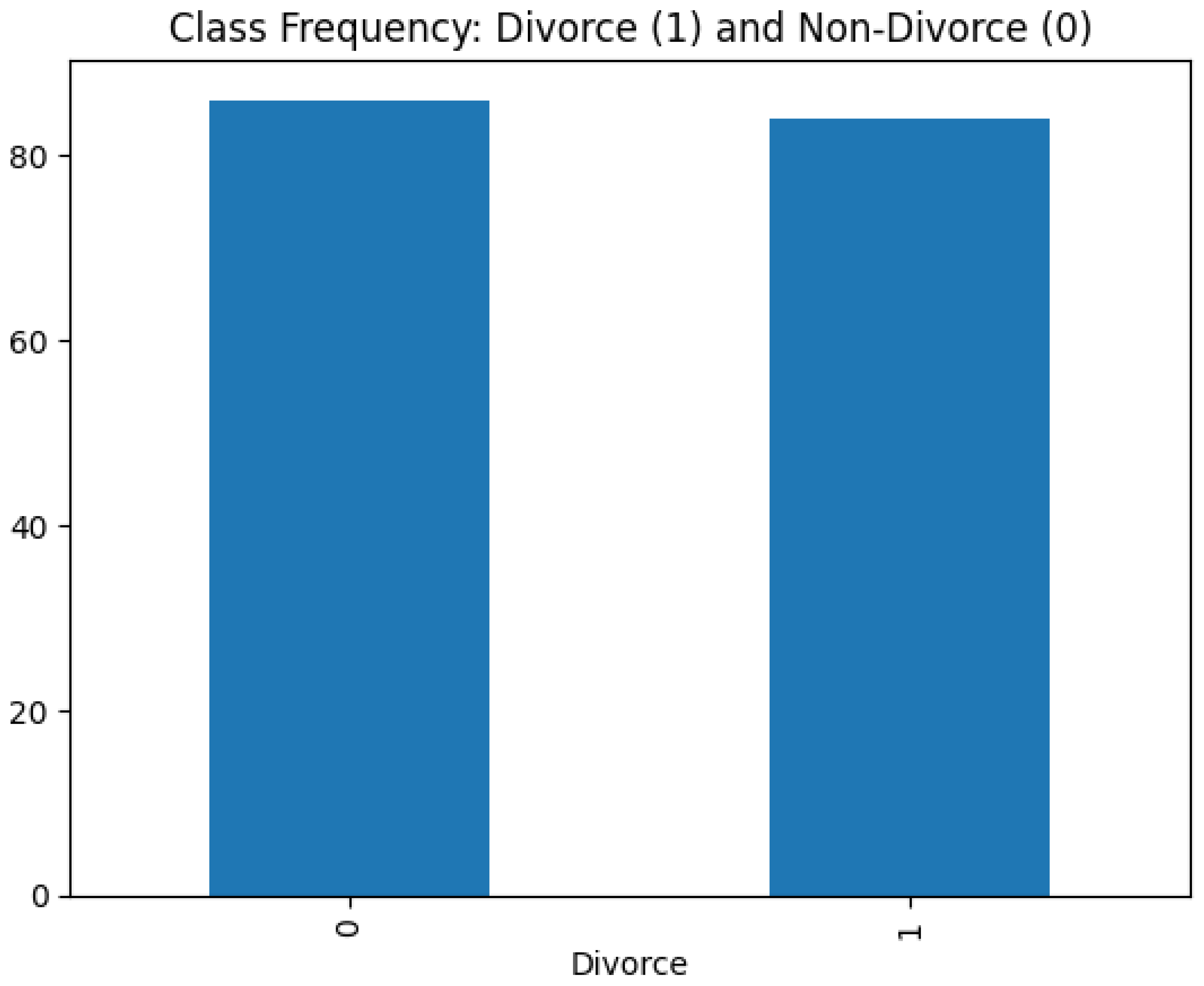
Figure 2.
ROC-AUC Curve of Each Model.
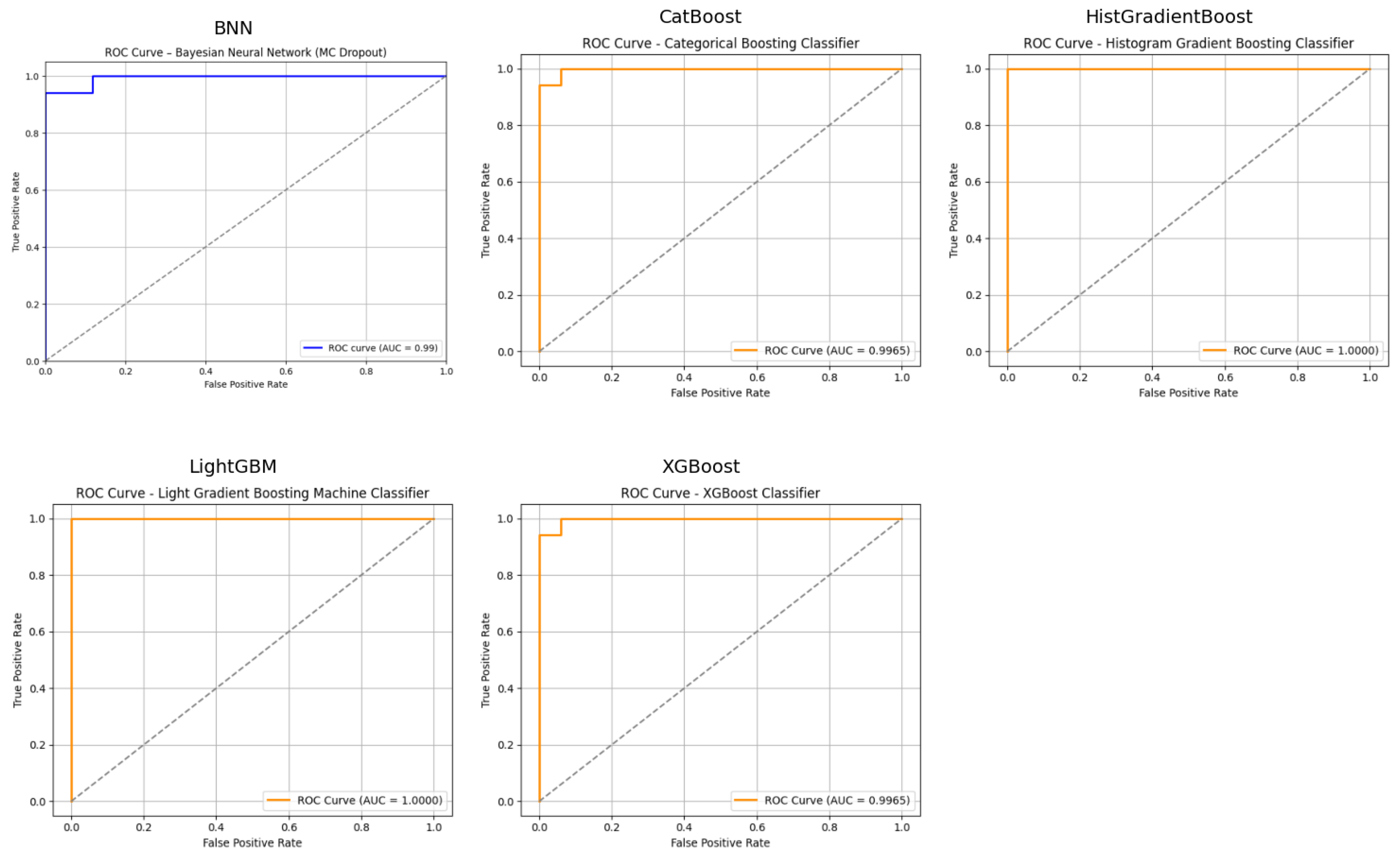
Figure 3.
SHAP Waterfall Plot (Local Interpretation of a Non-Divorce Instance).
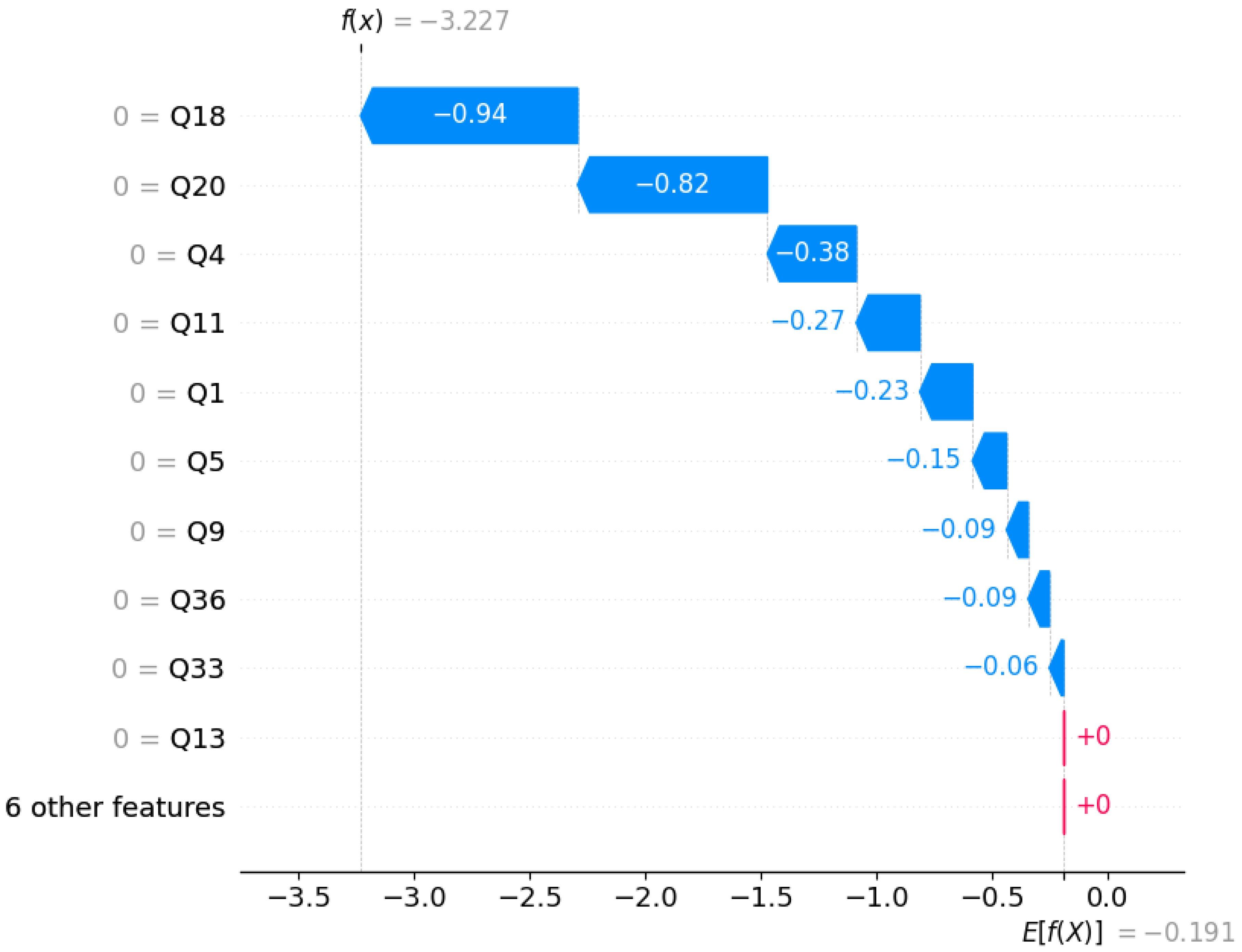
Figure 4.
SHAP Waterfall Plot (Local Interpretation of a Divorce Instance).
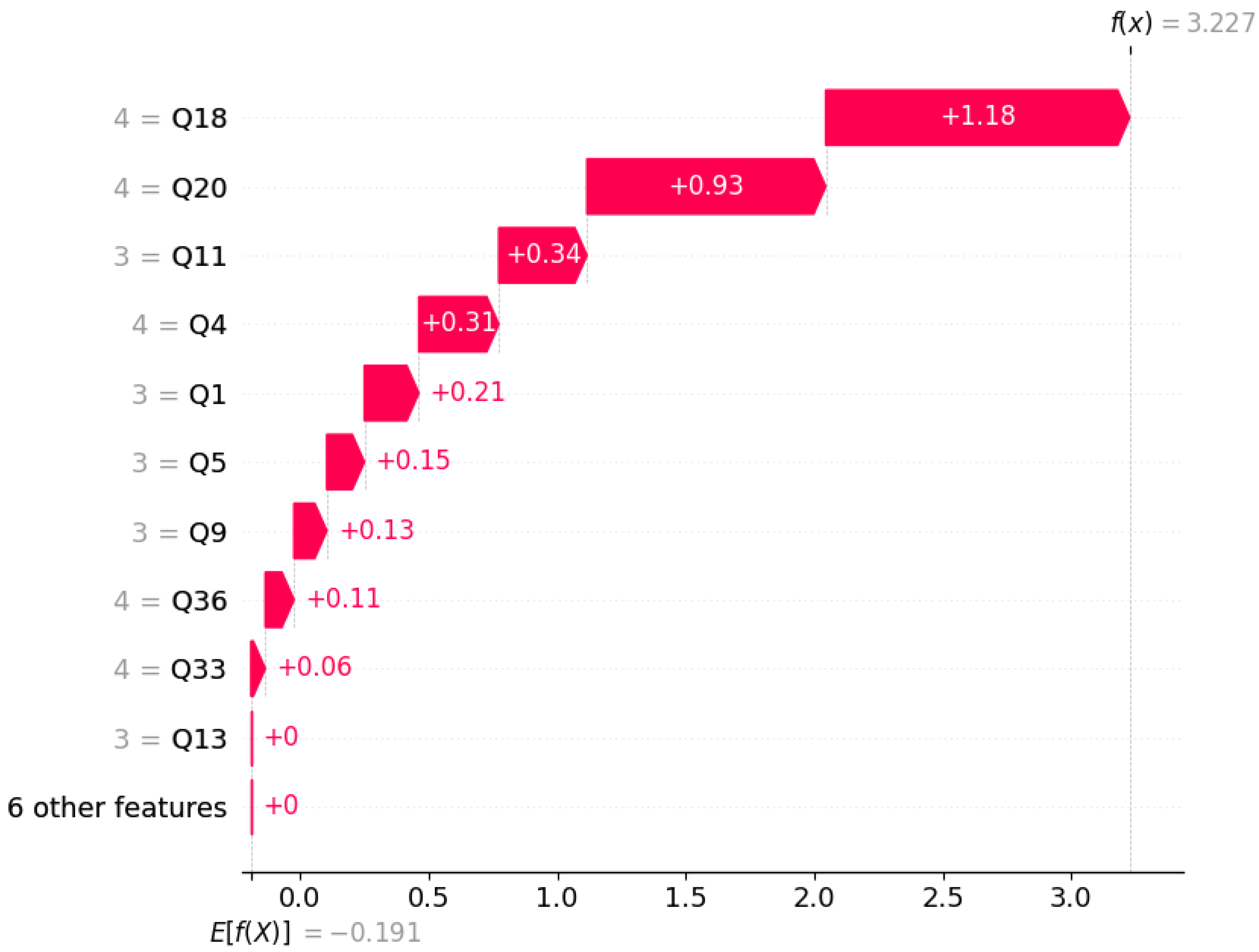
Figure 5.
SHAP Value as Global Interpretation (Impact on Model Output).
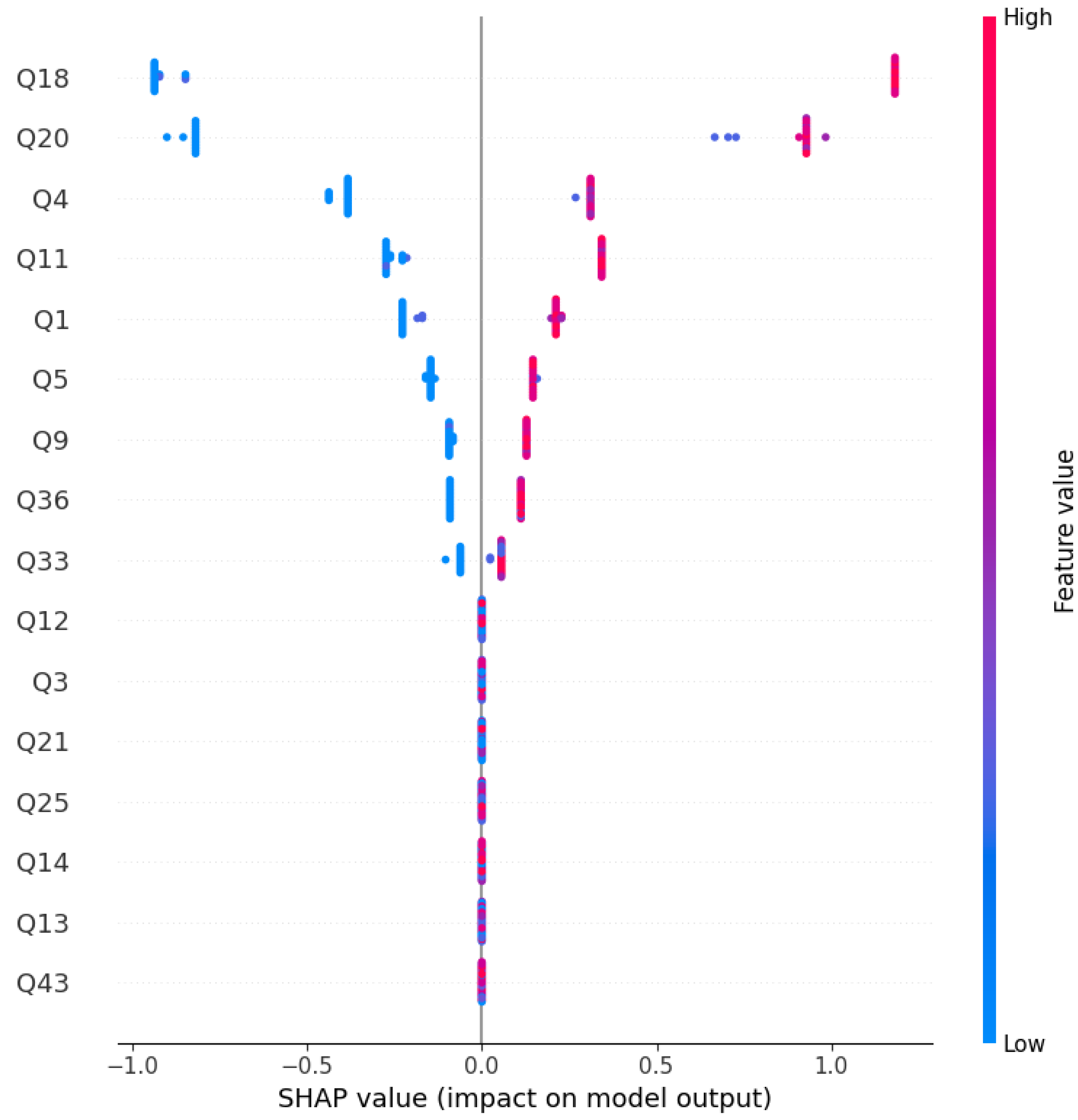
Figure 6.
Counterfactuals: No Divorce to Divorce.
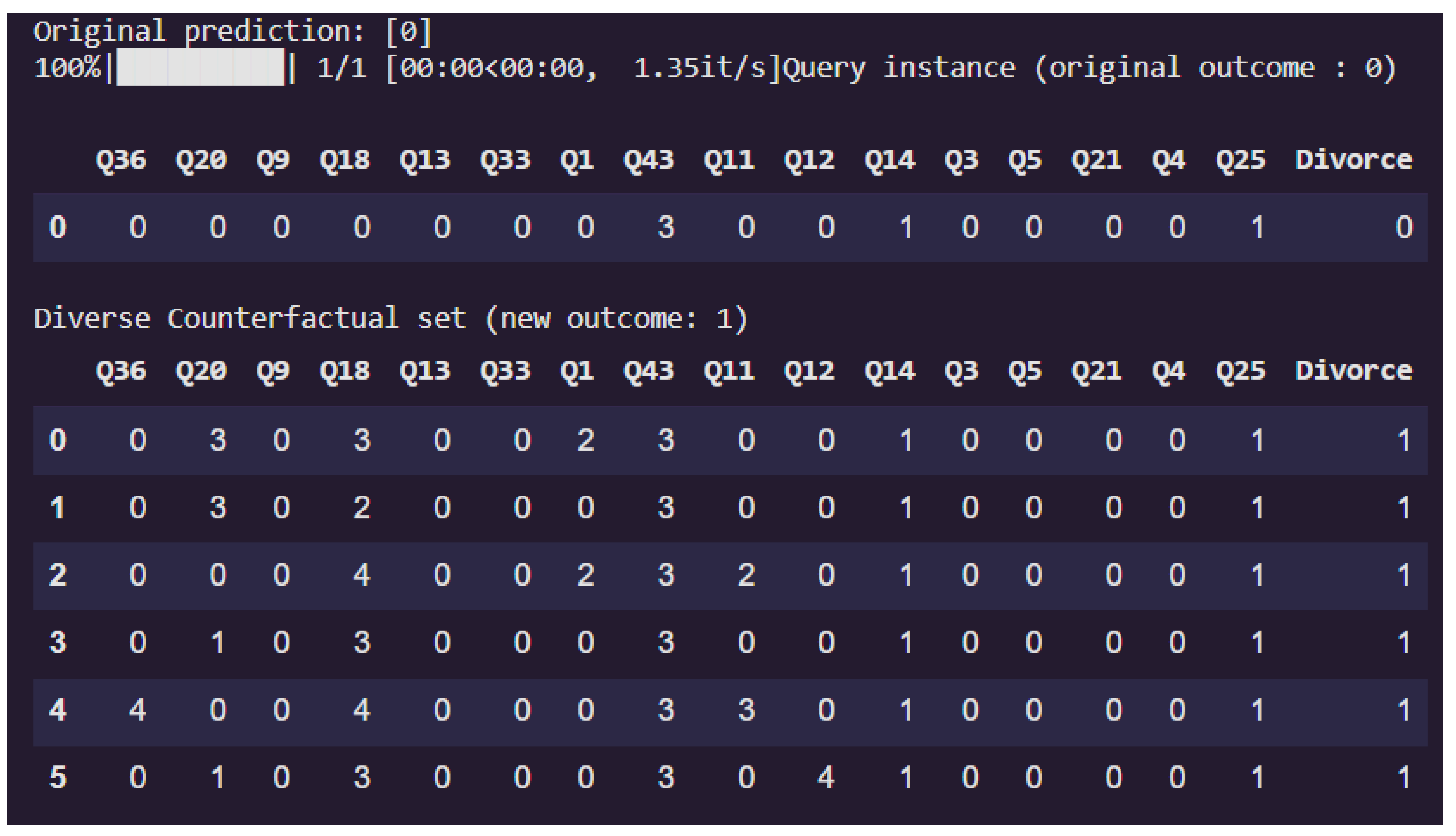
Figure 7.
Counterfactuals: No Divorce to Divorce.
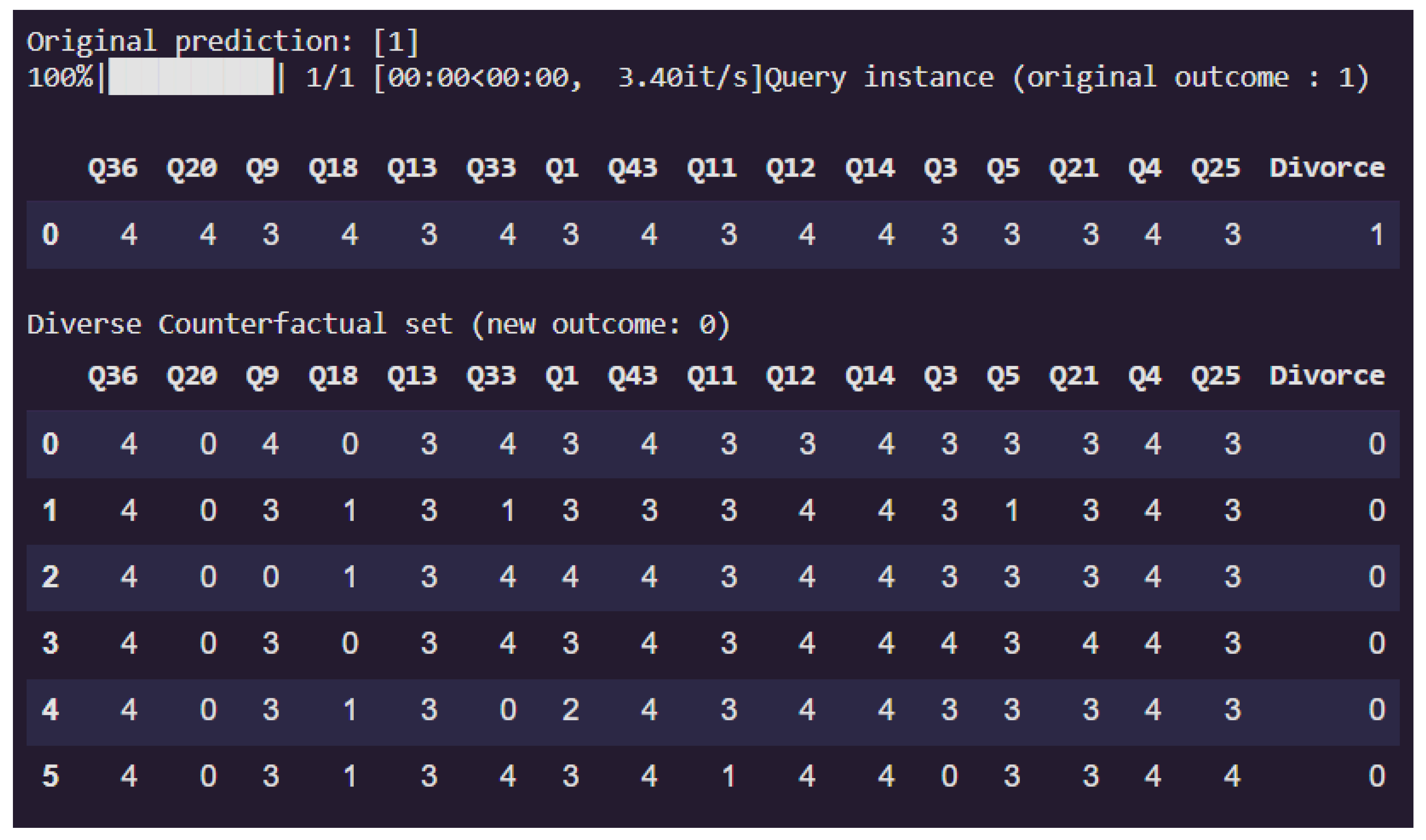
Figure 8.
Uncertainty in Predictions by BNN.
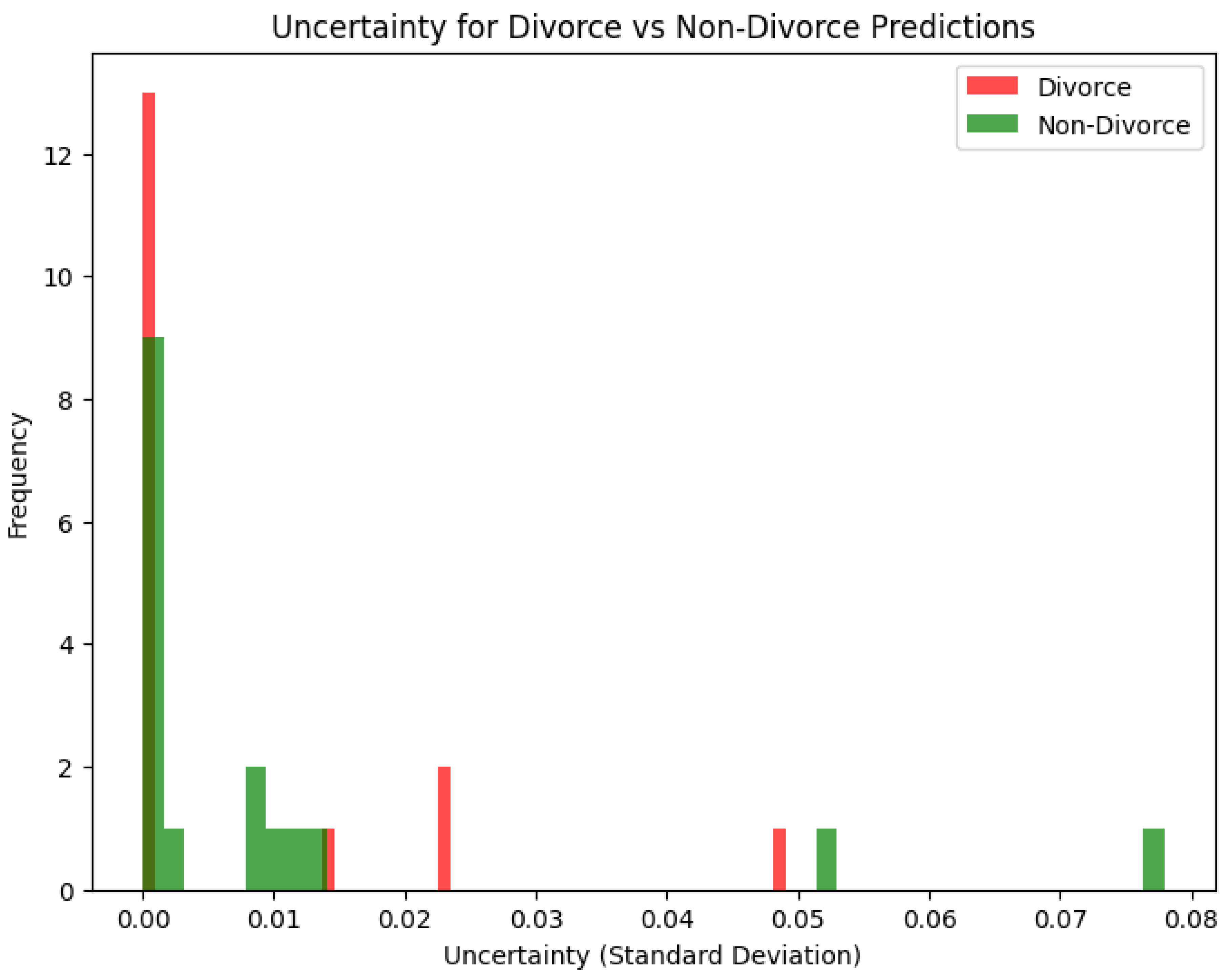
Figure 9.
Uncertainty Quantification for a Divorce Instance.
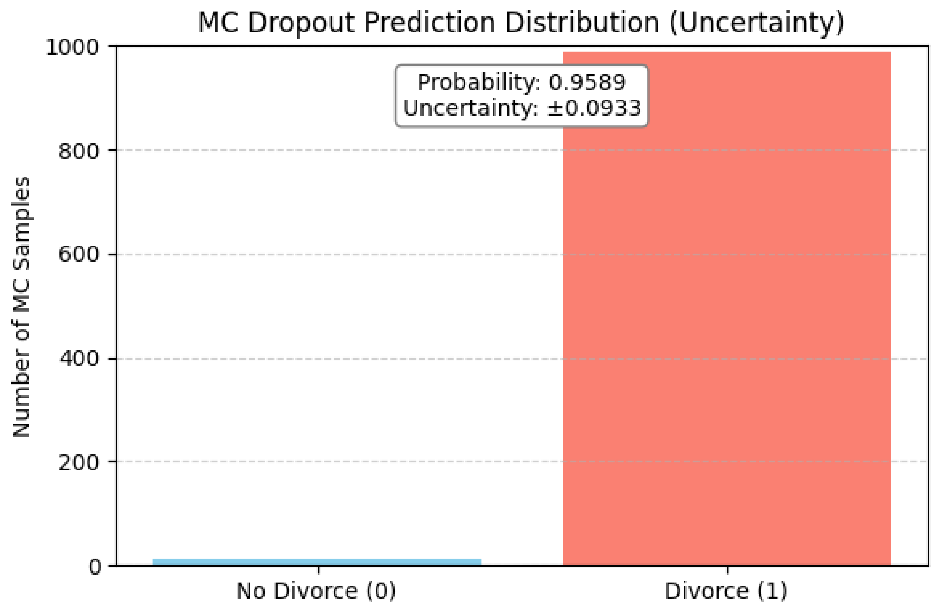
Figure 10.
Uncertainty Quantification for a Non-Divorce Instance.
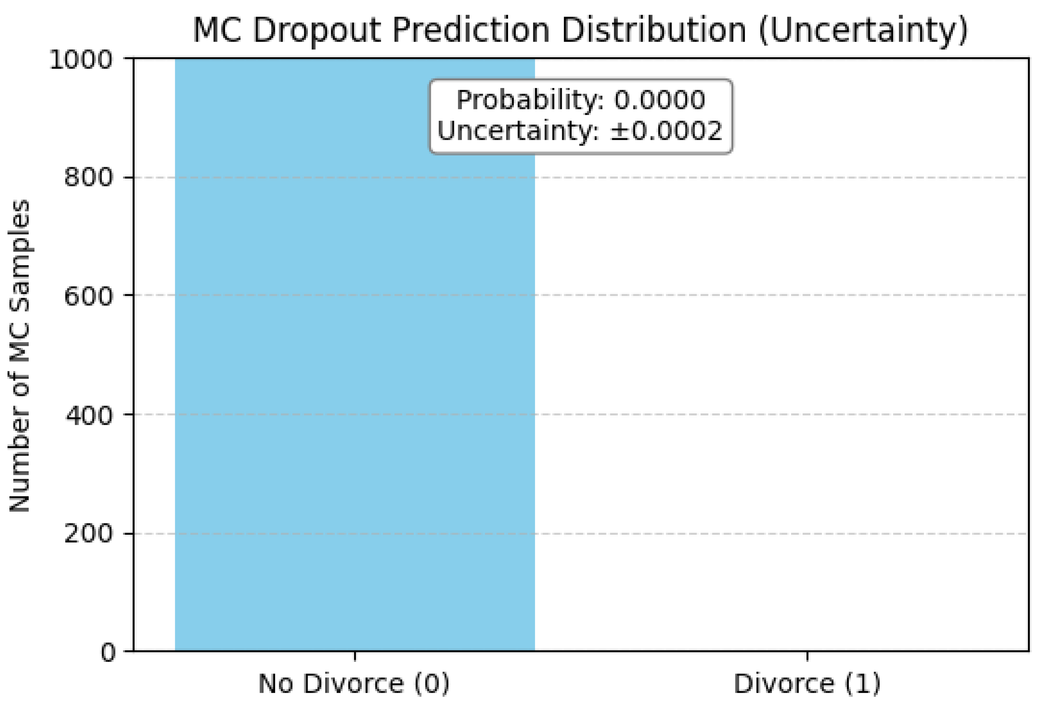

Table 1.
Top 16 causally influential features based on average treatment effect (ATE).
| Feature | Definition | ATE |
|---|---|---|
| Q36 | Can be humiliating when we discuss | 0.2440 |
| Q20 | Similar values in trust with spouse | 0.2399 |
| Q9 | Enjoy traveling with my wife | 0.2257 |
| Q18 | Similar ideas on how marriages should be | 0.2162 |
| Q13 | Have similar senses of entertainment | -0.2078 |
| Q33 | Can use negative statements on my spouse in discussions | -0.1881 |
| Q1 | Discussion ends when one of us apologizes | -0.1688 |
| Q43 | I stay silent to calm the environment | 0.1655 |
| Q11 | Nostalgia regarding harmony with wife | -0.1570 |
| Q12 | Similar values in terms of personal freedom | -0.1502 |
| Q14 | Most of our goals for people are same | 0.1404 |
| Q3 | Take the discussions with spouse from beginning and correct it | 0.1375 |
| Q5 | Time spent with my wife is special | 0.1322 |
| Q21 | I know what my wife likes | -0.1303 |
| Q4 | Contacting him eventually works, during discussion | 0.1281 |
| Q25 | I have knowledge on my spouse’s inner world | -0.1237 |
Table 2.
Model Performance Metrics.
| Model | Accuracy | Precision | Recall | F1-Score | ROC-AUC |
|---|---|---|---|---|---|
| XGBoost | 0.9797 | 0.9982 | 0.9612 | 0.9790 | 0.9972 |
| HistGBoost | 0.9759 | 0.9945 | 0.9576 | 0.9750 | 0.9978 |
| LGBM | 0.9672 | 0.9809 | 0.9724 | 0.9759 | 0.9985 |
| CatBoost | 0.9753 | 0.9926 | 0.9582 | 0.9745 | 0.9986 |
| BNN | 0.9411 | 0.9411 | 0.9411 | 0.9411 | 0.9930 |
Table 3.
Uncertainty Associated with the Performance Metrics (95% CI).
| Model | Accuracy | Precision | Recall | F1-Score | ROC-AUC |
|---|---|---|---|---|---|
| XGBoost | 0.0588 | 0.0309 | 0.1176 | 0.0625 | 0.0199 |
| HistGBoost | 0.0588 | 0.1053 | 0.1176 | 0.0625 | 0.0138 |
| LGBM | 0.0588 | 0.0608 | 0.1176 | 0.0625 | 0.0138 |
| CatBoost | 0.0588 | 0.0588 | 0.1176 | 0.0625 | 0.0069 |
Table 4.
Comparison of Divorce Prediction Models in Literature.
| Research | Models | Strength |
|---|---|---|
| [23] | KNN, SVM, Bi-LSTM | Performance (F1-score 0.932) |
| [26] | ANN, NB, RF | Performance (Accuracy 0.916) |
| Correlation-based feature selection | ||
| [24] | IndoBert, RF | Performance (Precision 0.82) |
| Oversampling | ||
| [25] | RF, Neural Network | Performance (AUC score 0.981) |
| 10-fold cross-validation | ||
| [28] | LR, GB, SVM, RF | Performance |
| SHAP Interpretation (Global) | ||
| [29] | LR, NB, SGD, DT, RF, MLP | Performance (Accuracy 1.0) |
| Information Gain, OneR-based feature selection | ||
| [30] | LR, LDA, KNN, CART, NB, SVM | Performance (Accuracy 0.9857) |
| LIME Interpretation (Local) | ||
| User-friendly App | ||
| [31] | AdaBoost, GB, XGBoost, RF | Performance (Accuracy 0.97) |
| WOA-based hyperparameter tuning | ||
| [27] | SVM | Accuracy 0.9823 |
| SHAP Interpretation (Global) | ||
| Ours | XGBoost, LGBM, CatBoost, HistGBoost, BNN | Performance (Accuracy 0.9797) |
| Causal inference-based feature selection | ||
| Counterfactuals | ||
| SHAP (Global+Local) | ||
| Uncertainty Estimation | ||
| User Applicability |
Table 5.
Performance comparison between our model and recent SOTA tabular models.
| Model | Accuracy | Precision | Recall | F1-Score |
|---|---|---|---|---|
| XGBoost | 0.98 | 0.99 | 0.96 | 0.98 |
| FT-Transformer | 0.97 | 1.00 | 0.94 | 0.97 |
| TabPFN | 0.94 | 1.00 | 0.88 | 0.94 |
| TabNet | 0.53 | 0.52 | 1.00 | 0.68 |
Disclaimer/Publisher’s Note: The statements, opinions and data contained in all publications are solely those of the individual author(s) and contributor(s) and not of MDPI and/or the editor(s). MDPI and/or the editor(s) disclaim responsibility for any injury to people or property resulting from any ideas, methods, instructions or products referred to in the content. |
© 2025 by the authors. Licensee MDPI, Basel, Switzerland. This article is an open access article distributed under the terms and conditions of the Creative Commons Attribution (CC BY) license (http://creativecommons.org/licenses/by/4.0/).
Copyright: This open access article is published under a Creative Commons CC BY 4.0 license, which permit the free download, distribution, and reuse, provided that the author and preprint are cited in any reuse.


