
Submitted:
08 May 2025
Posted:
09 May 2025
You are already at the latest version
Abstract
As road traffic in Turkey is a significant source of emissions due to the increasing number of vehicles on the road, the goal of this study is to calculate greenhouse gas emissions from Turkey roads between 2010 and 2020, as well as to create an inventory and estimate possible emissions until 2050. In the study, both primary greenhouse gases (carbon dioxide-CO2, and diazote oxide-N2O) and secondary greenhouse gases (ammonia-NH3, nitrogen oxide-NOX, sulfur dioxide-SO2, carbon monoxide-CO, non-methane volatile organic compounds-NMVOC, and particulate matter-PM) were investigated. The study showed that Turkey’s total number of vehicles using state roads increased by 60% between 2010 and 2020. As a result, emissions of CO2, N2O, NH3, NOX, SO2, CO, NMVOC, and PM increased by 29.6%, 24.2%, 0.5%, 19.9%, 9.9%, 18.2%, 21.5%, and 39.7%, respectively. When emissions were analyzed on a provincial basis, particular attention was drawn to provinces with high levels of urbanization. Based on forecast studies, it is predicted that the total number of vehicles registered in the traffic will increase by 105% by 2050. Due to this increase, CO2, N2O, NH3, NOX, SO2, CO, NMVOC and PM emissions are estimated to increase by 149.17%, 151.78%, 154.39%, 138.95%, 150.97%, 153.09%, 152.09% and 151.47%, respectively.
Keywords:
Climate change
; Greenhouse gas emissions
; Sustainability
; Traffic
; Emission Inventory
; Turkey
1. Introduction
According to the Intergovernmental Panel on Climate Change (IPCC), there is clear evidence that the climate system is undergoing a warming trend. This is supported by observations that indicate a global increase in the average temperatures of the air and oceans, widespread melting of snow and ice, and a rise in the global average sea level [1]. The primary driver of climate change is predominantly attributed to anthropogenic activities, particularly the combustion of fossil fuels. Manufacturing and transport sectors are significant contributors to greenhouse gas emissions. This gives rise to a worldwide issue that impacts the global population [2,3]. The Paris Agreement, adopted on December 12, 2015, and enforced on November 4, 2016, is significant in the international struggle against climate change. It relies primarily on the United Nations Framework Convention on Climate Change. The primary objective of the agreement is to minimize the rise in global temperature relative to the pre-industrial era to a level below 2 °C. This objective necessitates a decrease in the use of fossil fuels, and a transition toward the adoption of renewable energy sources. The paramount aspect of this agreement is the inclusion of both developed and developing nations in taking measures to reduce emissions through their Nationally Determined Contributions (NDCs).
Turkey agreed to the Paris Agreement in 2015, on the condition that its request for financial and technological assistance in the new climate framework was accomplished. It officially signed the agreement on April 22, 2016, declaring itself a "developing country," and formally became a participant in the Paris Agreement on 10 November 2021. Turkey has revised its reduction target in its Intended NDCs from 21% in 2015 to 41% in 2030. Turkey’s revised First NDCs encompasses the entirety of its economy and incorporates extensive measures for mitigation and adaptation, along with an evaluation of implementation mechanisms. Turkey aims to reach its highest emissions point by no later than 2038. The revised objective for mitigation is to achieve carbon neutrality by the year 2053, as indicated by references [4,5].
Due to developments in the transportation sector across numerous countries, there has been a notable rise in energy consumption and emissions, making the global effort to combat carbon emissions more challenging. Transport has generally become more efficient. Most vehicles emit less carbon dioxide per kilometer than previously. Their engines are more fuel efficient. But those gains have not kept up with growing transport volumes. More kilometers are traveled for business and holidays, and more cargo is carried. This is the main reason for total emissions from transport having increased [6]. On a global scale, the transportation industry accounts for 15% of overall greenhouse gas emissions and 23% of carbon dioxide emissions (CO2). Global emission data from transport networks shows that the road sector has the highest GHG emissions, accounting for approximately 74.5% of emissions from passenger and freight transport. Furthermore, passenger cars account for 80% of the energy consumption in land transport [7,8]. Turkish Statistical Institute (TurkStat) greenhouse gas emission inventory data for 2020 revealed that in Turkey, the most CO2 emissions from transport, precisely 94.9%, originated from road transportation. Air transportation accounts for 2.7% of emissions, maritime contributes 1.6%, railway contributes 0.4%, and other transport modes contribute 0.4% [9]. Transport emissions encompass not only carbon dioxide (CO2) and methane (CH4), which are the primary contributors to climate change, but also additional pollutants, such as particulate matter (PM), sulfur dioxide (SO2), and nitrogen oxides (NOX) [10].
Transportation plays a crucial role in sustainable development, as it relies heavily on fossil fuels and significantly contributes to carbon emissions, one of the leading GHGs. Furthermore, the transportation industry contributes to other adverse consequences, such as soil erosion, traffic congestion, air pollution, and ecosystem destruction. Hence, it is of the utmost importance to develop and execute sustainable transportation strategies. The first step is to identify the existing conditions. Once the situation is assessed, the subsequent stage involves making future projections and establishing the necessary goals and strategies. Because road traffic in Turkey is a significant source of emissions due to the increasing number of vehicles on the road, the goal of this study was to conduct an inventory and calculate the emissions of direct GHGs, namely CO2 and diazote oxide (N2O), as well as indirect GHGs, such as ammonia (NH3), NOX, SO2, CO, NMVOC, and PM, from vehicles travelling on Turkey state roads. At the same time, the purpose was to conduct a precise analysis of current emission levels as well as estimation studies for future emissions.
For the study, initially, information regarding the number of vehicles traversing state roads, their classifications, and the distances of the roads were acquired from the reports of the General Directorate of Highways (GDH) spanning 11 years from 2010 to 2020. As the data obtained from these reports are appropriate for using emission factors in the "EMEP/EEA (Emission Inventory Guidebook) air pollutant emission inventory guidebook 2023" database, Tier 1 emission factors in this database were used in the calculations. Quantum GIS (QGIS), an open-source geographic information system (GIS) software, was used to generate distribution maps based on emission amounts calculated with this database. In this way, the spatial arrangement of emissions from vehicular traffic traveling on state roads in Turkey was demonstrated. This study also used the polynomial regression method to analyze a dataset from the Turkish Statistical Institute (TurkStat). The dataset included the number of vehicles registered for traffic between 1966 and 2021. The analysis was performed using Python 3.7 coding. Based on this analysis, the expected number of vehicles by 2050 was estimated and the associated emissions that could be released were calculated.
It is hoped that this study will draw attention to the increasing emission amounts and contribute to other studies focusing on similar issues. In addition, it will be essential to consider this and similar studies when legislative authorities make emission reduction decisions. During a time when the impact of GHGs is particularly significant, it has been observed that the assessment of GHG emissions from vehicles on all state roads, excluding major cities, has not been adequately conducted. This study addresses the existing knowledge gap in literature.
2. Materials and Methods
2.1. Study Area
Turkey is located between 36°- 42° north-latitude and 26°- 45° east-longitude and acts as a bridge between Asia and Europe through the Bosporus and Dardanelles Straits. Due to the geographical position of the country, it is important as it is situated on trade, migration, and major east-west and north-south corridors [11]. The country's population increased from 56.47 million in 1990 to 84.68 million in 2021. The growth in population substantially influences the escalation in demand for housing, energy, and transportation, particularly in the urban regions of Turkey [12]. Based on the 2020 data, Turkey has a road network with a total length of 68,266 kilometers. This network comprises 5% (3095 km) motorways, 45.4% (31006 km) state roads, and 50.1% (34165 km) provincial roads [13]. Figure 1 displays a map of state roads in Turkey
The motor vehicle registration count experienced significant growth, rising from 15,095,603 in 2010 to 26,482,847 by 2022. Furthermore, when analyzed on the bases of fuel type, petrol car numbers rose from 3,191,964 to 3,817,104, diesel cars from 1,381,631 to 5,261,876, and LPG cars from 2,900,034 to 5,005,563 [15]. Despite an annual increase in the overall number of vehicles, car ownership in Turkey remains significantly lower than the European average, primarily because of exorbitant car prices and taxes. Based on the 2019 data, Luxembourg has a car ownership rate of 681 cars per thousand people, Italy has a rate of 663 cars per thousand people, and Turkey has a rate of 150 cars per thousand people. The average for the EU-27 in 2019 was 553 [16].
To compare the number of vehicles utilizing Turkey's state roads between 2010 and 2020, the Annual Average Daily Traffic (AADT) numbers for every section of Turkey's state roads were gathered. It was found that the total increased by 60% from 11,193,242 in 2010 to 17,917,138 in 2020 [17]. Although these total values (total AADT numbers) do not clearly show the number of vehicles using the roads, it is significant to notice the rise throughout the years. Because these increases also increase traffic-related emissions.
2.2. Emission Calculations
An approach commonly used to calculate traffic emissions is emission factors [10]. Emission factors are frequently employed to evaluate transport emissions by establishing a correlation between pollutant emissions and vehicle activities and types, such as distance traveled, fuel consumption, and energy consumption [18].
In this study, the number, type, and distance travelled on state roads in Turkey, which form the basis of emission calculations, were compiled from the traffic transport information index published annually by the GDH for the 11 years between 2010 and 2020 [17]. Vehicles were classified as automobiles (Personal Cars-PC), light commercial vehicles (LCV), and heavy-duty vehicles (HDV), and automobiles were classified as petrol, diesel, and LPG according to fuel type [15]. This study classified LCVs and HDVs in Turkey as diesel-fuelled vehicles because they mainly use diesel fuel with some exceptions. The study used Tier 1 emission factors specified for each pollutant according to vehicle and fuel types in the EMEP/EEA air pollutant emission inventory guidebook 2023. Calculations were made separately for each state road section in each province. Then the calculation results were collected for each province. The annual emission values for each pollutant were calculated using the method specified in Equation 1. The calculations employ emission factors from Table 1, and Table 2 displays the fuel consumption data per kilometer for each vehicle category.
Where E is the amount of emissions (kg/day), FCj,m is the fuel consumption (g-fuel/km), EFi,j,m is the emission factor (g/km).
Data on the distribution of registered cars based on fuel type is sourced from TurkStat for 11 years. The corresponding graph is shown in Figure 2.
2.3. Future Predictions
Within the scope of this study, the number of vehicles was predicted up to 2050 using the polynomial regression method using Python 3.7 coding. The accuracy of predicting future vehicle counts using the polynomial regression method is contingent on the breadth of the past information set. To make this estimate, there needs to be more than the dataset on the number of vehicles traveling on state roads in the study area, which is used for emission calculations. Therefore, the number of vehicles registered to traffic in Turkey between 1966 and 2021 from TurkStat is used in the estimation study. By analyzing the number of vehicles between 1966 and 2021, a projection was made for the period until 2050. This projection enabled the calculation of future emissions based on average per-vehicle emissions and emission factors defined in the EMEP/EEA air pollutant emissions inventory guide. For future emission predictions, GHG emissions were calculated on the bases of the number of vehicles using state roads, and average emissions per vehicle (Equation 2) were calculated considering the total number of vehicles. Then, from the average emission amounts per vehicle, emission estimates were made according to the number of vehicles estimated for the future.
Where MVE is the mean vehicle emissions (kg emission/per vehicle), n is the first year used in the calculation, p is the final year used in the calculation, Em is the calculated emission value (kg), and Veh is the number of vehicles.
This method provides a solid framework for forecasting future emissions and analyzing long-term trends. Using this and comparable predictive models may be valuable for generating future predictions.
2.4. Polynomial Regression
Regression is an essential topic in data mining that is employed to forecast a certain outcome by considering input factors. The data-driven model is unsuitable for linear prediction in some engineering computations. When faced with such situations, employing a suitable curve for the given data is advisable. Polynomial regression is a commonly employed method for data analysis [20,21]. It has an advantage over linear models by offering high flexibility in modeling non-linear data relationships. Thanks to its flexible structure, it can capture complex trends and shapes. So the model can fit the data better [22]. This method provides high accuracy in capturing nonlinear relationships and fitting curves, so it can represent more complex data relationships [23]. Polynomial regression learning too much data may cause overfitting. In this case, the model may perfectly predict the data it was trained on, but may fall short on new data. Additionally, outliers can seriously degrade the accuracy of the model. It is also important to determine the appropriate polynomial degree; Lower degrees may be insufficient, while higher degrees may create unnecessary complexity. Therefore, these factors should be carefully considered when creating a model [23,24].
Polynomial regression is a specific instance of multiple regression involving a single independent variable, denoted as X. The formula below represents the univariate polynomial regression model. K represents the degree of the polynomial. The degree of the polynomial is a parameter that quantifies the model's intricacy level. Effectively, this is equivalent to having a multiple model with the variables X1 = X, X2 = X2, X3 = X3, and its formula is expressed in Equation 3 [25].
𝑦𝑖 = 𝛽0 + 𝛽1𝑥𝑖 + 𝛽2𝑥𝑖 2 + 𝛽3𝑥𝑖 3 . . .+𝛽𝑘𝑥𝑖 𝑘 + 𝜀𝑖, for 𝑖 = 1,2, . . . , 𝑛
Where y is the dependent variable, x is the independent variable, k is the polynomial degree, β0, β1, …, βk are constant coefficients, εi is the error between the model and the observations.
The coefficient of uncertainty is calculated using Eq. (4). Where R2 is the coefficient of uncertainty. This value is used to show the relationship between variables. The variable takes a value between 0 and 1 when calculated using the foregoing formula. The nearness of R2 to 1 indicates good agreement between the values.
Where St is the total sum of squares and Sr is the residual sum of squares [26].
3. Results
3.1. Greenhouse Gas Emission Calculations from State Roads
This study examined the emissions of direct GHGs, primarily CO2 and N2O, and indirect GHGs, including NH3, NOX, SO2, CO, NMVOC, and PM, which contribute to the indirect greenhouse effect. The calculations were performed for 11 years from 2010 to 2020. The results obtained are given in Table 3.
When the results of the study are evaluated (Table 3), the amounts of CO2, N2O, NH3, NOX, SO2, CO, NMVOC, and PM increased by 29.6%, 24.2%, 0.5%, 19.9%, 9.9%, 18.2%, 21.5%, and 39.7%, respectively, in 11 years. Of all the contaminants, the PM pollutant showed the highest increase of 39.7%, while the NH3 pollutant showed the smallest increase of 0.5%. This situation relates to the types of fuel used by vehicles. An analysis of fuel types of vehicles used in traffic reveals that diesel cars, LPG-fueled cars, LCVs, and HDVs have had growth rates of 3.60, 1.64, 2.06, and 1.15 times, respectively, during 11 years. In contrast, petrol cars have seen a decline of 0.82%. Diesel-fueled automobiles, LCVs and HDVs collectively account for almost 50% of all vehicles on the road. While diesel-powered cars produce more PM emissions than petrol-powered vehicles, petrol-powered vehicles emit more NH3 emissions than diesel-powered vehicles [19]. Consequently, while the type and quantity of emissions vary depending on the fuel used, the dominance of oil as the primary fuel in the transportation sector is highly significant. When the literature is reviewed, the increases in traffic-related greenhouse gas emissions in Turkey and other nations are noteworthy [27-31]. To mitigate the rise in GHG emissions, one practical approach is to impose restrictions on the use of fossil fuels. To achieve carbon neutrality across every sector and transportation, the European Union has declared its intention to prohibit the sale of diesel and petrol automobiles entirely by 2035 [32]. Nevertheless, the rate at which the automobile sector in Turkey is adapting to this transition is unclear. Anticipating its global ubiquity is an inaccurate perspective. Fluctuations and advances in the transportation industry are diverse. It is recommended to use a lot of preventive applications to provide higher precision in reaching the desired effect.
Upon analyzing the emission values calculated, a consistent rise was evident between 2010 and 2018 (Table 3). However, between 2018 and 2020, the levels of CO2, N2O, NH3, NOX, SO2, CO, NMVOC, and PM reduced by 3.9%, 6.4%, 8%, 5.3%, 6.3%, 8.5%, 8.1%, and 4.4%, respectively. The decrease in the number of cars on the roadways covered in the research may be attributed to the impact of lockdown restrictions and reduced vehicle traffic during the pandemic. Specifically, vehicles decreased from 19,379,148 in 2018 to 19,132,034 in 2019 and 17,917,138 in 2020. This unequivocally demonstrates the outcome of minimizing automobile usage through practices such as remote working and abstaining from daily commuting to and from the workplace. Furthermore, the construction of highways, tunnels, and bridges to enhance the efficiency, cost-effectiveness, sustainability, and environmental friendliness of road transportation across the nation may also have a positive impact. The road network, which was 62,864 km in the early 2000s, has increased to 68,266 km in the 2020s, and the number of tunnels increased from 83 to 488 [13]. Therefore, part of the reduction in emissions in these years can also be attributed to reduced distances travelled.
Figure 3 displays the distribution of overall GHG emissions between 2010 and 2020, originating from vehicles that were in transit on the roadways included in the research, categorized by vehicle type. Automobiles account for 58% of all emissions. When assessing pollutant sources, PCs are shown to be responsible for 65% of N2O, 95% of NH3, 59% of SO2, 86% of CO, and 77% of NMVOC pollutants. In contrast, HDVs accounted for 52% of CO2, 74% of NOX, and 67% of PM pollutants. Given that diesel fuel is used as the primary source of energy in HDVs, it would be advantageous to implement fuel-oriented enhancements to mitigate the emission of CO2, NOX, and PM pollutants.
To analyze the spread of emissions from automobiles on state highways in Turkey, emission distribution maps for 2010 and 2020 were generated using QGIS. The resulting maps are shown in Figure 4. The charts clearly illustrate that the emission levels in 2010 were more significant in the Western and Central Anatolia. Furthermore, it is evident that emissions further increased by 2020. The results are summarized item by item below:
- The daily CO2 ranged from 47.8 to 2429 kg in 2010 and increased from 98.74 to 3024.8 kg in 2020. In 2010, Konya province had the highest recorded CO2 emissions. In contrast, Ankara province had the highest values reported in 2020.
- The daily N2O in 2010 ranged from 1.21 to 69.53 kg/day, whereas in 2020, they ranged from 1.72 to 97.94 kg/day. Emissions were significantly elevated, particularly in central Turkey. In 2010, the province with the highest emission amount was Bursa; in 2020, it was Antalya.
- The daily CO ranged from 406.06 to 26,895.91 kg/day in 2010 and from 599.12 to 34,543.22 kg/day in 2020. In 2010, Antalya province had the highest recorded emission amount. In 2020, it was Ankara.
- NH3 was calculated in the range of 2.75-196.82 kg/day in 2010 and 3.63-209.54 kg/day in 2020. The highest emission quantity was calculated in Antalya in 2010 and Ankara in 2020.
- When NMVOC levels were examined, values ranged between 64.83 and 4030.7 kg/day in 2010. Antalya has the highest calculated emission. In 2020, there was a change between 94.42 and 5436.84 kg/day and the highest emission calculated in Ankara.
- NOX amounts were calculated as 330.67-19470.02 kg/day and 446.55-25733.49 kg/day for 2010 and 2020, respectively. The calculated max. emission amounts were the Konya and the Ankara, respectively.
- The daily quantity of PM10 was calculated to be 9.20–551.12 kg in 2010 and 15.51–835.51 kg in 2020. The provinces of Konya and Ankara were calculated to have the highest maximum emission quantities for 2010 and 2020, respectively.
- In Turkey, the amount of SO2 emissions was calculated to be 0.35–20.19 kg/day in 2010 and 0.44–25.30 kg/day in 2020. Antalya (in 2010) and Ankara (in 2020) were determined to have the highest maximum emission quantities.
Based on the calculations, while there are variations in emissions levels throughout the provinces, the cities of Ankara, Antalya, and Bursa consistently exhibit the highest rises in emissions. This might be attributed to the rise in population and subsequent increase in vehicular traffic in these cities. Between 2010 and 2022, the population of Ankara increased from 4,771,716 to 5,782,285, that of Antalya climbed from 1,978,333 to 2,688,004, and that of Bursa increased from 2,605,495 to 3,194,720 [12].
Fast population expansion leads to rapid urbanization. During the evaluation of provinces for the year 2020, Istanbul, with a population density of 2427 people per square kilometer, Kocaeli, with a population density of 454 people per square kilometer, and Izmir, with a population density of 324 people per square kilometer, ranked as the top three provinces in terms of population density. Tunceli has a population density of 10 people per square kilometer and has the lowest population density among these provinces. The provinces of Bursa, Ankara, and Antalya, which see the highest increases in emissions, are rated 7th (241 individuals per square kilometer), 9th (186 individuals per square kilometer), and 23rd (97 individuals per square kilometer). Kocaeli province ranks top in GHG emissions per square kilometer, with values of 5056 g/km2 for CO, 475 g/km2 for CO2, 14 g/km2 for N2O, 32 g/km2 for NH3, 3 g/km2 for SO2, and 778 g/km2 for NMVOC. Yalova province ranks first in NOX emissions (3365 g/km2) and PM emissions (112 g/km2). Bilecik has the highest per capita GHG emissions for CO, CO2, N2O, NH3, NOX, PM, SO2, and NMVOC, with values of 31, 4, 0.1, 0.2, 37, 1, 0.03 , and 5 g/person, respectively. These provinces are characterized by a high degree of urbanization. Urbanization results in environmental degradation, pollution, physical disorganization, and anomalies in settlement. Sustainability plays a crucial role in the growth and development of cities. To achieve the environmental goals of sustainability, urban design should include the characteristics of the local climate, ecosystems, energy, water, and resource movements. This planning approach aims to incorporate communities into the natural environment, decrease reliance on vehicles, optimize resource utilization, and showcase the area’s unique characteristics [33].
3.2. Future Predictions
This study used the polynomial regression approach to predict the number of vehicles up to the year 2050. The findings of this analysis are presented in Figure 5. Equations used for predicting future outcomes;
PC : y = - 23542263.54 x1 + 5963.80 x2 + 23233610555.34 (R² = 0.996) (5)
LCV : y = -10136215.80 x1 + 2562.45 x2 + 10023901731.90 (R² = 0.985) (6)
HDV : y = -1077353.36 x1 + 275.54 x2 + 1053131321.99 (R² = 0.967) (7)
Where y is the dependent variable (number of vehicles in the future), x is the independent variable (number of vehicles in the past).
The registered vehicle count, which stood at 26,482,847 at 2022, is projected to have grown by 105%, reaching 50,701,935 by 2050. The projected figures indicate that there will be 34,855,102 PCs, 13,344,351 LCVs, and 2,502,482 HDVs.
There are different methods for estimation in literature. Irhami and Farizal [34] estimated the number of vehicles in Indonesia using the ARIMA (Auto Regressive Integrative Moving Average) method. The estimate for the next 11 years was based on historical data from 2001 to 2019. As a result of the research, the best estimation models were determined as ARIMA (1,1,0) for cars and ARIMA (2,1,2) for motorcycles. The article explains that a rising number of automobiles generates a variety of difficulties such as traffic congestion, air pollution, and traffic accidents, and underlines the need of predicting the number of vehicles in the future in order to avoid such problems [34]. Sekula et al. [35] used machine learning (ML) and vehicle measurement data to estimate historical hourly traffic levels on Maryland's road network. The study was aimed at improving correctly predict hourly traffic volumes in areas with few sensors. In addition to the current profiling approach, a model was created using an artificial neural network (ANN). This technology produces 24% more accurate volume estimations than the profiling method utilized throughout the United States [35]. Sayed et al. [36] conducted a comprehensive evaluation of machine learning (AI)-based approaches for traffic flow prediction. The study focuses on Intelligent Transportation Systems (ITS) and the impact of machine learning (ML) and deep learning (DL) techniques used in these systems on traffic prediction. The difficulties observed in implementing these techniques were discussed in the paper [36]. Alhindawi et al. [37] estimated greenhouse gas (GHG) emissions from the road transportation sector in North America using multivariate regression and double exponential smoothing (DES) models. The purpose of the research was to contribute to the development of strategic decisions to minimize GHG emissions by calculating existing and future emissions. The results revealed that kilometers traveled and the number of vehicles have a substantial impact on greenhouse gas emissions [37].
According to studies, the number of vehicles on the road is going to rise steadily. This means a rise in emissions. Turkey implemented EURO 5 standards in October 2009 and EURO 6 standards in January 2015 with the aim of decreasing pollution levels in newly manufactured vehicles. In 2021, an analysis of registered vehicles by age group revealed that 23.1% fall under the 0-5 years range, 24.6% fall within the 6-10 years range, 15.8% fall within the 11-15 years range, 10.2% fall within the 16-20 years range, and 26.3% are older than 21 years [38]. Hence, while these norms will partially regulate the pace of emission growth, more is needed. Therefore, emissions predictions were also made based on the number of vehicles that were estimated up to 2050. The graphs are shown in Figure 6. Upon analyzing Figure 6, it becomes evident that each emission type has a consistent upward tendency as time passes. The ratios for CO2, N2O, NH3, NOX, PM10, SO2, CO, and NMVOC are 149.17%, 151.78%, 154.39%, 138.95%, 151.47%, 150.97%, 153.09%, and 152.09%, respectively. External factors such as future technological developments, changes in economic conditions, or policy interventions that could significantly affect future vehicle use and emissions may suggest that emissions increases will not occur at this rate. However, there were also developments between 2010 and 2020, and despite these developments, an increase in emissions was observed. The effectiveness of existing emission reduction policies between these years was not sufficient to reduce emissions. From this perspective, it is thought that the results of study reflects the developments in the transportation sector and environmental policy environment, and that there will be emission increases at these rates in the future under current conditions. Due to the rise in GHG emissions, there is a growing concern about global climate change. This poses a potential danger to the ecosystem and living organisms, leading to extreme conditions such as changes in precipitation, humidity, air movement, and temperature. Therefore, it is necessary to implement stricter environmental regulations, penalties, and policies, to shift towards alternative transportation modes, or urban planning changes that could alter vehicle usage patterns to address this issue. There are studies in the literature that produce recommendations for reducing greenhouse gas emissions. For example, Doğan Güzel and Alp [39] conducted a study to analyze the effects of the transport sector on climate change in Istanbul, the most populous city in Turkey, with a high vehicle density. They used a model to estimate GHG emissions from 2016 to 2050. They employed the Integrated Markal-EFOM System (TIMES), a technologically advanced and cost-effective model to achieve this objective. In addition, they examined three different possibilities concerning electric rail transportation (Scenario 1), electric and hybrid vehicles (Scenario 2), and restricted CO2 emissions (Scenario 3). The findings indicated that by 2050, Scenario 1 would result in a 1.1% decrease in GHG emissions, Scenario 2 would lead to an 11% reduction, and Scenario 3 would achieve a significant 39% decrease [39].
The literature discusses seven primary themes for achieving sustainable transportation by mitigating GHG emissions. Strategies to achieve these goals include the use of alternative fuels, promotion of fuel-efficient vehicles, decrease in vehicle use, reduction of transportation infrastructure, implementation of intelligent transport systems, integration of various modes of transportation, and reduction of overall travel [40]. These issues primarily encompass strategies aimed at mitigating or, at the very least, limiting the release of GHG emissions throughout the lifespan. GHG emissions are also generated during the manufacturing and application phases. To effectively minimize GHG emissions, it is important to consider further options for raw material supply/production, mixture/road design, and casting/compaction procedures at this stage. GHG emissions from road building in China have been evaluated using the life cycle assessment approach at both the national and provincial levels, and these calculations have been performed independently from the use of fossil fuels. Chen et al. [41] highlighted the need for increased focus on GHG emissions associated with road construction. The study also investigated the impact of various factors on GHG emissions, such as the construction of concrete and asphalt roads, road classification, number of lanes, and road length. It also highlighted the presence of GHG emissions during the pre-service period of the road, which included the application phase starting from raw material production [41]. These studies demonstrate the importance of addressing the whole issue comprehensively and considering all its dimensions.
Türkiye needs to immediately implement several measures to achieve its goal, which it stated at the 27th Conference of the Parties (COP 27) in addressing climate change. Although sophisticated technology and low emissions are essential, it is important to acknowledge that our nation’s sluggish pace of vehicle replacement may delay the noticeable effects of new technology vehicles on overall emissions. To meet the desired objectives soon, it may be imperative to enforce financial measures and incentives to encourage the removal of vehicles manufactured with outdated technology from the current traffic fleet. This may promote a transition toward more efficient motor vehicles. Furthermore, increasing the number of absorption zones can reduce the country’s emissions by capturing and storing them. Based on Ministry statistics, approximately 9% of the country’s CO2 equivalent emissions were effectively captured and decreased in wooded regions, spanning around 23 million hectares in 2020. The sequestration patterns in 2020 exhibited a 3% rise compared with the data from 1990. [38,42]. It may be advantageous to further increase this growth rate.
4. Conclusions
The present study showed that there is significant and rapid growth in vehicle numbers using Turkey's roads. Turkey’s total vehicle numbers using state roads was 11,193,242 in 2010 but had risen to 17,917,138 by 2020, representing a 60% increase. The increasing number of vehicles in the transportation sector has led to an increase in fossil fuel consumption and, consequently, greenhouse gas emissions. The analysis showed percentage increases of 29.6%, 24.2%, 0.5%, 19.9%, 9.9%, 18.2%, 21.5%, and 39.7% for CO2, N2O, NH3, NOX, SO2, CO, NMVOC, and PM, respectively, between 2010 and 2020. Upon closer examination of the 11-year timeframe, particularly in 2020, the first full year of the COVID-19 epidemic, an average reduction of 5% in emission levels was observed compared with the preceding year. Implementing quarantine measures in response to the COVID-19 epidemic reduced emissions. The construction of highways, tunnels and bridges had a positive effect as they reduced the distance travelled. Thus, the positive results of increasing alternative transportation networks and reducing traffic mobility, even for a short time, were observed.
58% of all pollutants originating from vehicles were found to be automobile-related. However, 52% of CO2, an important greenhouse gas, was determined to be from HDVs. These vehicles use diesel fuel. This situation clearly showed the need of fuel-related changes.
When the calculated emission quantities by province were studied, Ankara, Antalya, and Bursa were determined to be the three cities with the highest emissions, despite several variances. The Kocaeli and Yalova provinces were rated worst regarding GHG emissions per square kilometer, whereas the Bilecik province was determined the most significant GHG emission per person. The increase in emissions was a result of urbanization and the increasing number of vehicles. Therefore, governments are advised to develop strategies to reduce emissions from transportation, particularly targeting large cities.
Based on the future forecasting study, there was a projected 50,701,935 registered vehicles in 2050, a 105% increase from the current figure. The rise in emissions was computed as follows: 149.17% for CO2, 151.78% for N2O, 154.39% for NH3, 138.95% for NOX, 151.47% for PM10, 150.97% for SO2, 153.09% for CO, and 152.09% for NMVOC; this depends on the number of vehicles. These rates reflect the situation in which all developments, measures and policies implemented between 2010 and 2020. Transportation infrastructure plays a crucial role in the correlation between energy and emissions. It is essential to highlight that energy consumption contributes to the rise of specific GHG emissions, specifically CO2. As a result, stronger environmental standards and regulations must be implemented in order to lessen the association between transportation frequency and greenhouse gas emissions.
Limitations of the Study
This study is limited to state roads with a rate of only 45.4% of the total. Provincial roads comprise 50.1% of the total, nevertheless nevertheless were excluded since there are no vehicle statistics for these roads. Similarly, motorways, which account for 5% of the total, were excluded because of their low proportion. However, the motorways are very heavily used so when considering the emissions generated by traffic on these motorways, it is reasonable to state that the emissions from transportation in Turkey on all types of roads exceed those computed in this study by more than twice.
Author Contributions
Ş.Ç.D: Investigation, Methodology, Writing-review & editing; K.O.D.: Data Editing, Programming using Quantum GIS and Python 3.7.; S.V.Ç.: Investigation, Data Editing, Writing-original draft.
Funding
The authors declare that no funds, grants, or other support were received during the preparation of this manuscript.
Institutional Review Board Statement
Not applicable.
Informed Consent Statement
Not applicable.
Data Availability Statement
Traffic volume data were downloaded from the website https://www.kgm.gov.tr/Sayfalar/KGM/SiteTr/Trafik/TrafikHacimHaritasi.aspx. Everyone can access to the traffic volume data.
Conflicts of Interest
The authors declare no conflicts of interest..
Abbreviations
The following abbreviations are used in this manuscript:
| CO2 | carbon dioxide; |
| N2O | diazote oxide; |
| NH3 | ammonia; |
| NOX | nitrogen oxide; |
| SO2 | sulfur dioxide; |
| CO | carbon monoxide; |
| NMVOC | non-methane volatile organic compounds; |
| PM | particulate matter; |
| IPCC | intergovernmental panel on climate change; |
| NDCs | determined contributions; |
| GHG | greenhouse gas; |
| LPG | Liquid petroleum gas; |
| EMEP/EEA | European Monitoring and Evaluation Programme/European Environment Agency; |
| GDH | General Directorate of Highways; |
| GIS | geographic information system; |
| TurkStat | Turkish Statistical Institute; |
| AADT | Annual Average Daily Traffic; |
| PC | Personal Cars |
| LCV | light commercial vehicles; |
| HDV | heavy duty vehicles. |
References
- EEA, European Environment Agency. About climate change. 2016, Retrieved , 2019. https://www.eea.europa.eu/tr/themes/climate/about-climate-change. 31 January.
- Jaroszweski, D.; Chapman, L.; Petts, J. Assessing the potential impact of climate change on transportation: the need for an interdisciplinary approach. Journal of Transport Geography 2010, 18, 331–335. [Google Scholar] [CrossRef]
- Carlsson Kanyama, A.; Carlsson Kanyama, K.; Wester, M.; Snickare, L.; Söderberg, I. L. Climate change mitigation efforts among transportation and manufacturing companies: The current state of efforts in Sweden according to available documentation. Journal of Cleaner Production 2018, 196, 588–593. [Google Scholar] [CrossRef]
- DCC, Directorate of Climate Change, Repuclic of Turkey Ministry of Environment, Urbanization and Climate Change. Republic of Türkiye Updated First Nationally Determined Contribution, 2024,Retrieved January 30, 2024. https://unfccc.int/sites/default/files/NDC/2023-04/T%C3%9CRK%C4%B0YE_UPDATED%201st%20NDC_EN.pdf.
- DCC, Directorate of Climate Change, Repuclic of Turkey Ministry of Environment, Urbanization and Climate Change. Paris Agreement, 2024, Retrieved January 30, 2024. https://iklim.gov.tr/en/paris-agreement-i-117.
- EEA, European Environment Agency. High time to shift gear in transport sector, 2023, Retrieved August 29, 2023. https://www.eea.europa.eu/signals-archived/signals-2022/articles/high-time-to-shift-gear.
- IPCC, Intergovernmental Panel on Climate Change. IPCC Sixth Assessment Report. Chapter 10: Transport, 2021, Retrieved , 2021. https://www.ipcc.ch/report/ar6/wg3/chapter/chapter-10/. 30 January.
- IEA, International Energy Agency. Tracking Transport 2020, Retrieved January 30, 2021. https://www.iea.org/energy-system/transport.
- RTMEUCC, Repuclic of Turkey Ministry of Environment, Urbanization and Climate Change. Greenhouse Gas Emission by Transportation Type, 2024, Retrieved January 30,, 2024. https://cevreselgostergeler.csb.gov.tr/%20ulastirma-turune-gore-seragazi-emisyonu-i-85790.
- Ku, A.; Kammen, D. M.; Castellanos, S. A quantitative, equitable framework for urban transportation electrification: Oakland, California as a mobility model of climate justice. Sustainable Cities and Society 2021, 74, 103179. [Google Scholar] [CrossRef]
- MD, Mınıstry of Development. Eleventh Development Plan, 2018, Retrieved January 30, 2024. https://www.guvenlitrafik.gov.tr/kurumlar/guvenlitrafik.gov.tr/Karayolu_Trafik_Guvenligi_Calisma_Grubu_Raporu.pdf.
- TP, Turkey Population, 2023, Retrieved January 30, 2024. https://www.nufusu.com/.
- GDH, General Directorate of Highways. General Directorate of Highways from Past to Present, 2023, Retrieved , 2024. https://www.kgm.gov.tr/Sayfalar/KGM/SiteTr/Root/default.aspx. 30 January.
- GDH, General Directorate of Highways. Maps, 2021, Retrieved January 30, 2022. https://www.kgm.gov.tr/SiteCollectionImages/KGMimages/Haritalar/turistik.jpg.
- TurkStat, Turkish Statistical Enstitute. Motor Vehicles, 23. Retrieved January 30, 2024. https://data.tuik.gov.tr/Bulten/Index?p=Motorlu-Kara-Ta%C5%9F%C4%B1tlar%C4%B1-Ocak-2023-49433&dil=1. 20 January.
- RTMEUCC, Repuclic of Turkey Ministry of Environment, Urbanization and Climate Change. Number of Motorized Land Vehicles, 2024, Retrieved January 30, 2024. https://cevreselgostergeler.csb.gov.tr/motorlu-kara-tasiti-sayisi-i-85797.
- GDH, General Directorate of Highways, Ministry of Transport and Infrastructure. Traffic and Transportation Information, 2021, Retrieved January 31, 2022. https://www.kgm.gov.tr/Sayfalar/KGM/SiteTr/Trafik/TrafikveUlasimBilgileri.aspx.
- Seo, J.; Park, J.; Park, J.; Park, S. Emission factor development for light-duty vehicles based on real-world emissions using emission map-based simulation. Environmental Pollution 2021, 270, 116081. [Google Scholar] [CrossRef] [PubMed]
- EMEP/EEA, European Environment Agency, Air pollutant emission inventory guidebook 2019. Publications Office of the European Union. Retrieved January 30, 2021. https://www.eea.europa.eu/publications/emep-eea-guidebook-2019/part-b-sectoral-guidance-chapters/1-energy/1-a-combustion/1-a-3-b-i/view.
- Sarkodie, K.; Fergusson-Rees, A.; Abdulkadir, M.; Yaw Asiedu, N. Gas-liquid flow regime identification via a non-intrusive optical sensor combined with polynomial regression and linear discriminant analysis. Annals of Nuclear Energy 2023, 180, 109424. [Google Scholar] [CrossRef]
- Shi, M.; Hu, W.; Li, M.; Zhang, J.; Song, X.; Sun, W. Ensemble regression based on polynomial regression-based decision tree and its application in the in-situ data of tunnel boring machine. Mechanical Systems and Signal Processing 2023, 188, 110022. [Google Scholar] [CrossRef]
- Singh, K. P.; Gupta, S.; Kumar, A.; Shukla, S. P. Linear and nonlinear modeling approaches for urban air quality prediction. Science of the Total Environment 2012, 426, 244–255. [Google Scholar] [CrossRef]
- Iqbal, A. M. Application of Regression Techniques with their Advantages and Disadvantages. Elektron Magazine 2020, 4, 11–11. [Google Scholar]
- Shanock, L. R.; Baran, B. E.; Gentry, W. A.; Pattison, S. C.; Heggestad, E. D. Polynomial Regression with Response Surface Analysis: A Powerful Approach for Examining Moderation and Overcoming Limitations of Difference Scores. Journal of Business and Psychology 2010, 25, 543–554. [Google Scholar] [CrossRef]
- Ajona, M.; Vasanthi, P.; Vijayan, D.S. Application of multiple linear and polynomial regression in the sustainable biodegradation process of crude oil. Sustainable Energy Technologies and Assessments 2022, 54, 102797. [Google Scholar] [CrossRef]
- Aslan, V.; Eryilmaz, T. Polynomial regression method for optimization of biodiesel production from black mustard (Brassica nigra L.) seed oil using methanol, ethanol, NaOH, and KOH. Energy 2020, 209, 118386. [Google Scholar] [CrossRef]
- Mbandi, A.M.; Malley, C.S.; Schwela, D.; Vallack, H.; Emberson, L.; Ashmore, M.R. Assessment of the impact of road transport policies on air pollution and greenhouse gas emissions in Kenya, Energy Strategy Reviews 2023, 49, 101120. [CrossRef]
- Civelekoğlu, G.; Bıyık, Y. Investigation of Carbon Footprint Change Originated from Transportation Sector. Bilge International Journal of Science and Technology Research 2018, 2, 157–166. [Google Scholar] [CrossRef]
- Türkay, M. Karayolu ulaşımından kaynaklanan sera gazı emisyonunun (karbon ayak izinin) hesaplanması: Eskişehir ili örneği. (Master Thesis). Cumhuriyet University, 2018 https://tez.yok.gov.tr/UlusalTezMerkezi/tezDetay.jsp?id=h_oND-zFpEPniNFRp8KCtw&no=z7z8rI4ek1lfdPBfXH2JGQ.
- Yang, C.; McCollum, D.; McCarthy, R.; Leighty, W. Meeting an 80% reduction in greenhouse gas emissions from transportation by 2050: A case study in California. Transportation Research Part D: Transport and Environment 2009, 14, 147–156. [Google Scholar] [CrossRef]
- Soruşbay, C.; Ergeneman, M.; Pekin, M. A.; Kutlar, A.; Arslan, H. Greenhouse Gas Emissions from Road Transport: Assessment of the Situation in Turkey. National Symposium on Air Pollution and Control, 2008, Retrieved January 30, 2024. http://hkadtmk.org/Bildiriler/HKK-2008/bildiriler/Soru%C5%9Fbay.pdf.
- EP, European Parliament. EU Ban on the Sale of New Petrol and Diesel Cars From 2035 Explained, 2022, Retrieved January 31, 2024. https://www.europarl.europa.eu/topics/en.
- Tosun, K. E. The analysis of compact city model in the process of sustainable urban development. Dokuz Eylul University the Journal of Graduate School of Social Sciences 2013, 15, 103–120. [Google Scholar]
- İrhami, E. A.; Farizal, F. Forecasting the number of vehicles in Indonesia using auto regressive integrative moving average (ARIMA) method. Journal of Physics: Conference Series 2021, 1845, 012024. [Google Scholar] [CrossRef]
- Sekuła, P.; Marković, N.; Vander Laan, Z.; Farokhi Sadabadi, K. (2018). Estimating historical hourly traffic volumes via machine learning and vehicle probe data: A Maryland case study. Transportation Research Part C: Emerging Technologies 2018, 97, 147–158. [Google Scholar] [CrossRef]
- Sayed, A. S.; Abdel-Hamid, Y.; Hefny, H. A. Artificial intelligence-based traffic flow prediction: A comprehensive review. Journal of Electrical Systems and Information Technology 2023, 10. [Google Scholar] [CrossRef]
- Alhindawi, R.; Abu Nahleh, Y.; Kumar, A.; Shiwakoti, N. Projection of greenhouse gas emissions for the road transport sector based on multivariate regression and the double exponential smoothing model. Sustainability 2020, 12, 9152. [Google Scholar] [CrossRef]
- RTMEUCC, Repuclic of Turkey Ministry of Environment, Urbanization and Climate Change. Ingested Areas and Carbon Sequestration, 2024, Retrieved January 31, 2024, https://cevreselgostergeler.csb.gov.tr/yutak-alanlar-ve-karbon-tutumlari-i-85723.
- Doğan Güzel, T.; Alp, K. Modeling of greenhouse gas emissions from the transportation sector in Istanbul by 2050. Atmospheric Pollution Research 2020, 11, 2190–2201. [Google Scholar] [CrossRef]
- Demirtürk, D. Studies towards reducing greenhouse gas effect in sustainable transportation. Journal of Engineering Sciences and Design 2021, 9, 1080–1092. [Google Scholar] [CrossRef]
- Chen, J.; Zhao, F.; Liu, Z.; Ou, X.; Hao, H. Greenhouse gas emissions from road construction in China: A province-level analysis. Journal of Cleaner Production 2017, 168, 1039–1047. [Google Scholar] [CrossRef]
- Habib, Y.; Xia, E.; Hashmi, S. H.; Ahmed, Z. The nexus between road transport intensity and road-related CO2 emissions in G20 countries: an advanced panel estimation. Environmental Science and Pollution Research 2021, 28, 58405–58425. [Google Scholar] [CrossRef] [PubMed]
Figure 1.
Turkey roads map [14].
Figure 1.
Turkey roads map [14].
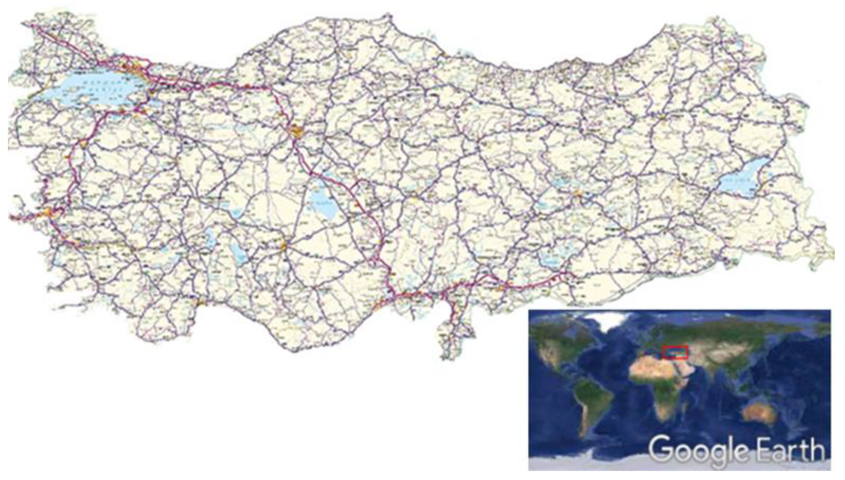
Figure 2.
Classification of registered vehicles in Turkey on the basis of fuel type [15].
Figure 2.
Classification of registered vehicles in Turkey on the basis of fuel type [15].
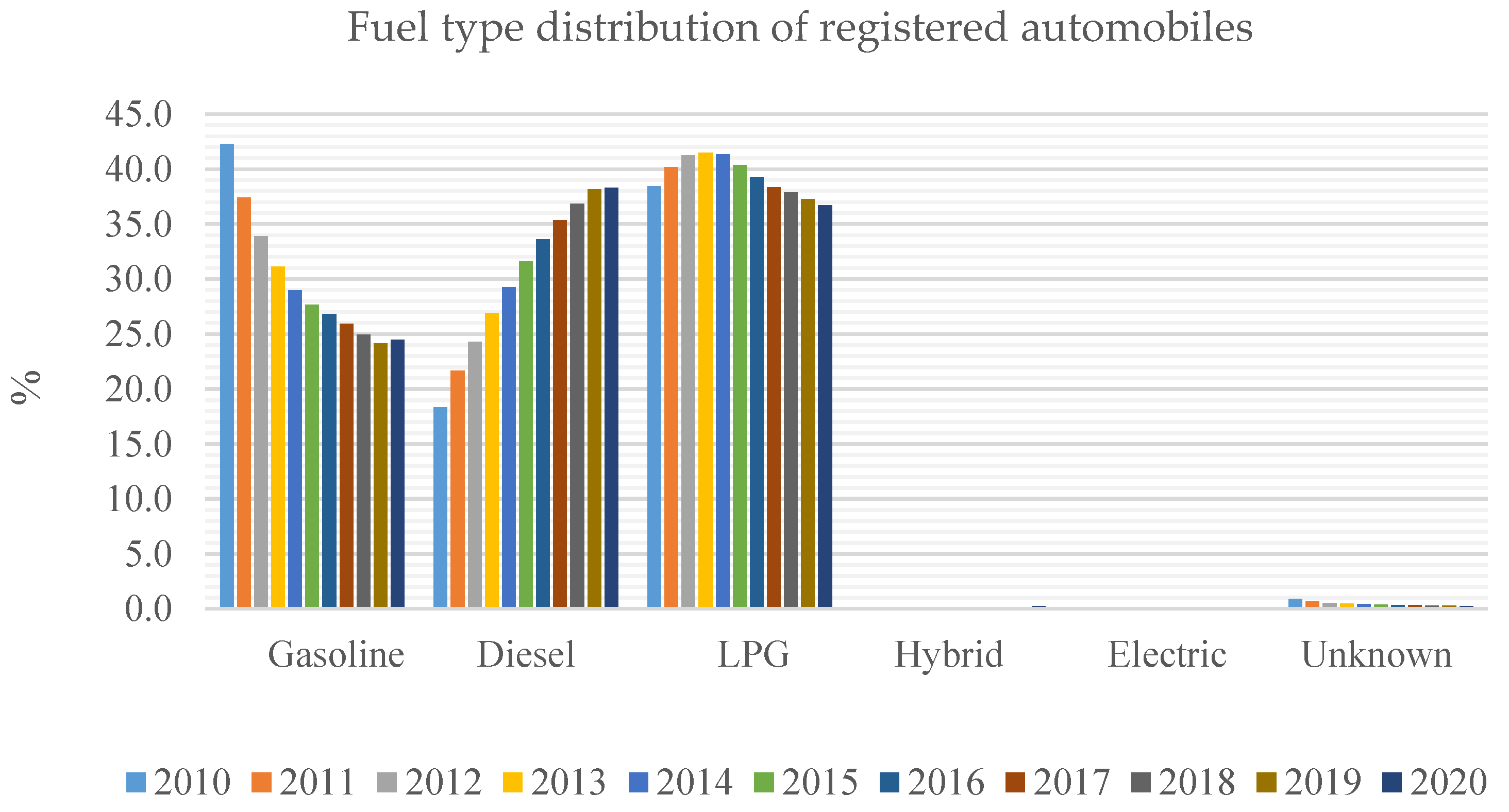
Figure 3.
Distribution of total vehicle-based GHG emissions on state roads in Turkey from 2010 to 2020 by vehicle type.
Figure 3.
Distribution of total vehicle-based GHG emissions on state roads in Turkey from 2010 to 2020 by vehicle type.
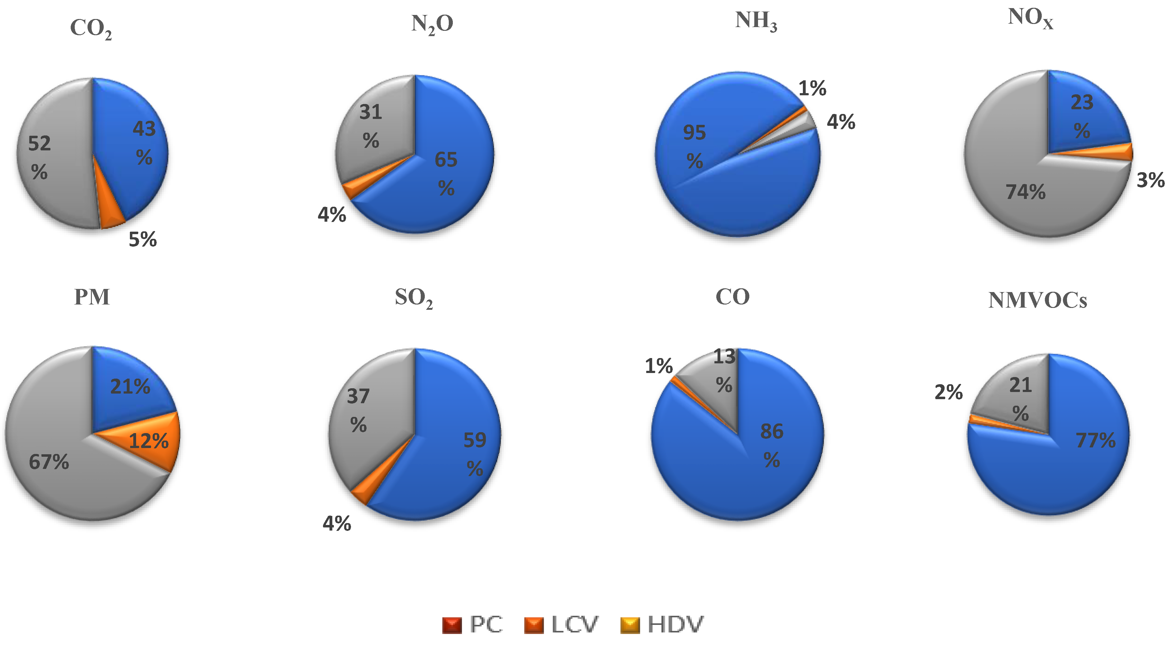
Figure 4.
Distribution of emissions from vehicles traveling on state roads in Turkey (A:2010 and B:2020).
Figure 4.
Distribution of emissions from vehicles traveling on state roads in Turkey (A:2010 and B:2020).
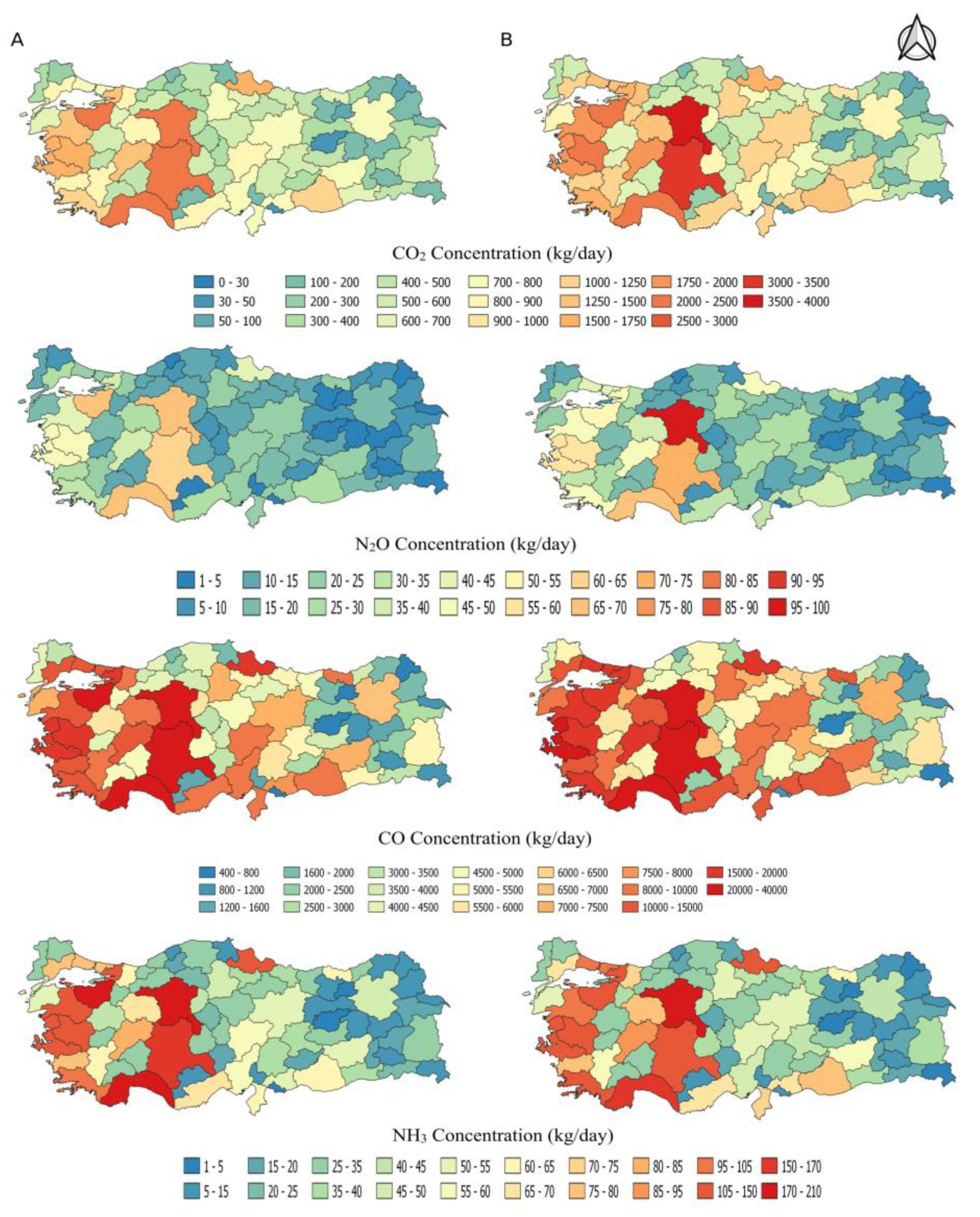
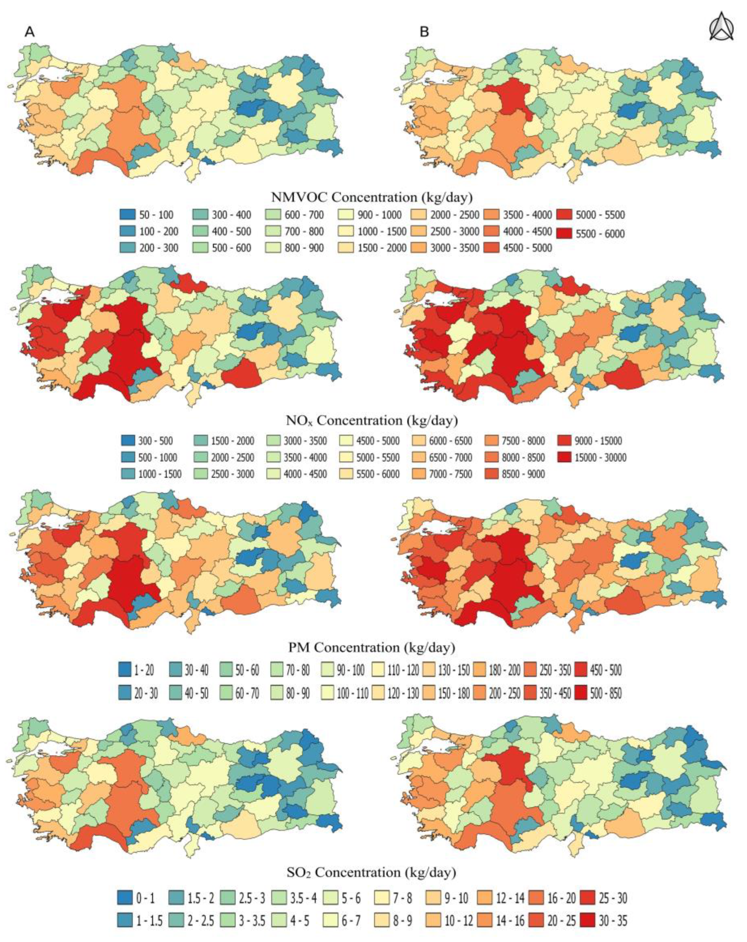
Figure 5.
Polynomial regression vehicle projections for the future.
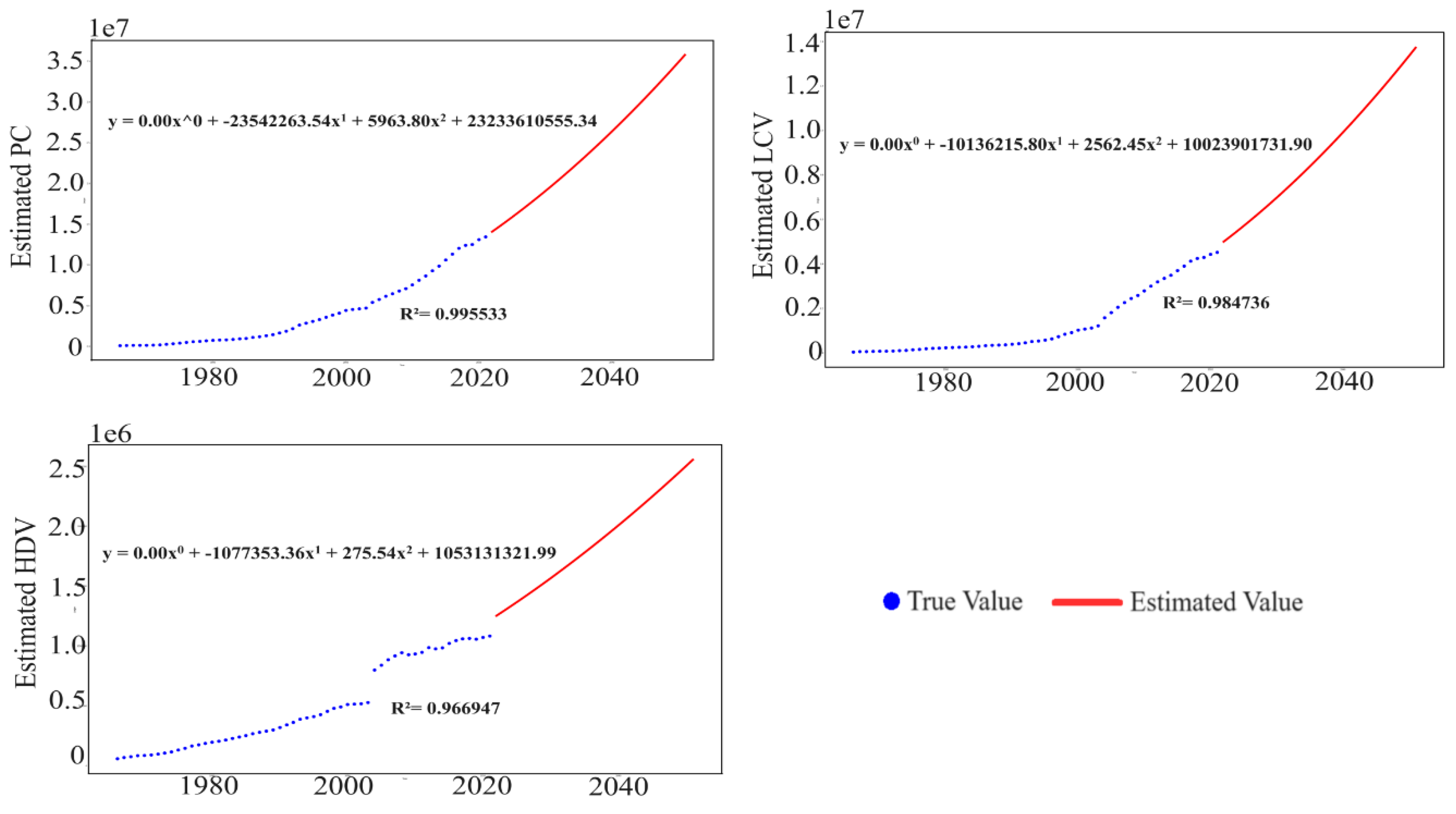
Figure 6.
Vehicle-based emission estimates for the future.
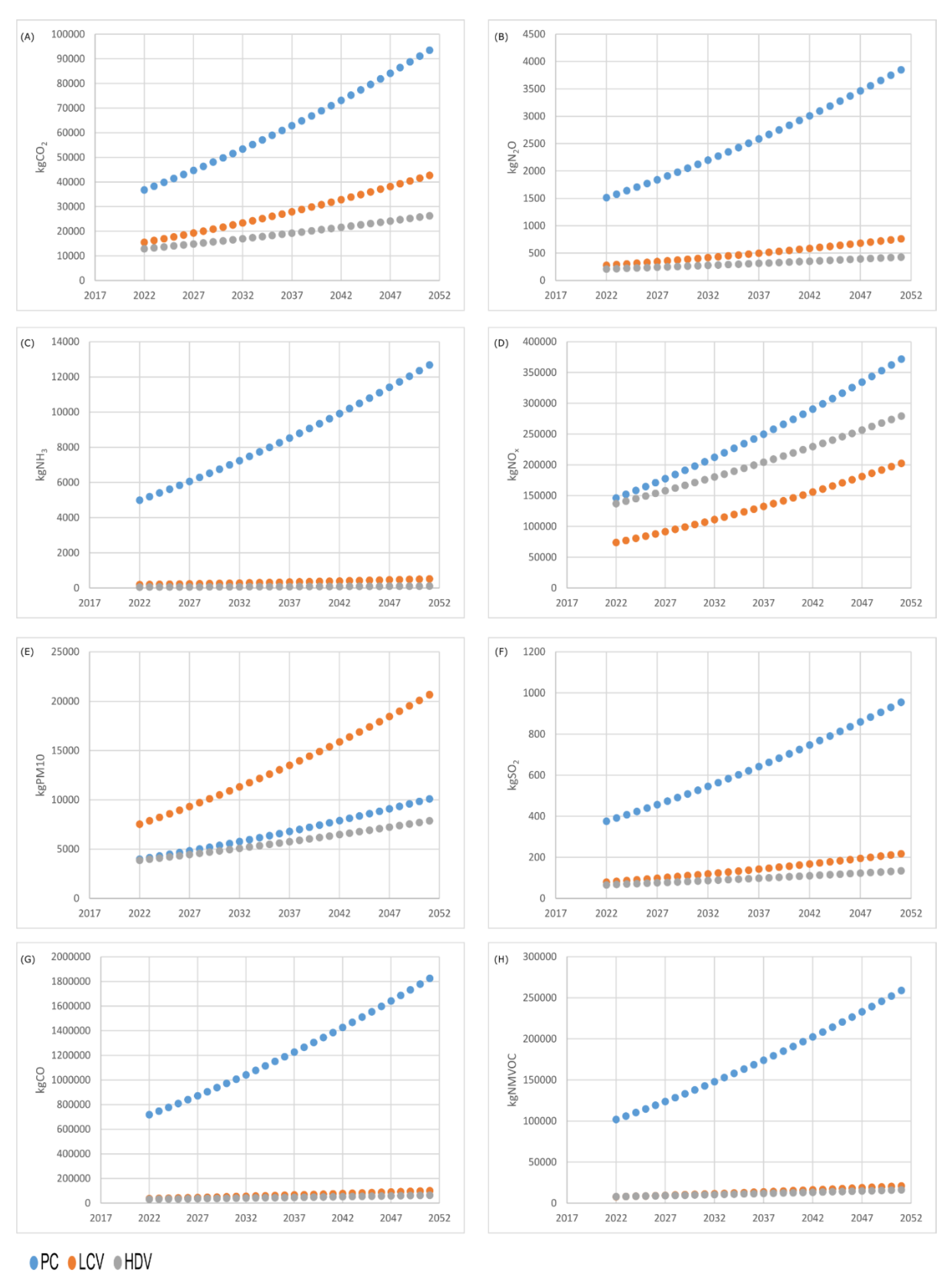

Table 1.
Tier 1 emission factors [19].
Table 1.
Tier 1 emission factors [19].
| Emission | Automobile g/kg | HDV g/kg | LCV g/kg | ||
|---|---|---|---|---|---|
| Gasoline | Diesel | LPG | Gasoline | Diesel | |
| CO | 84.7 | 3.33 | 84.7 | 7.58 | 7.4 |
| CO2 | 3.18 | 3.14 | 3.017 | 3.14 | 3.14 |
| SO2 | 0.08 | 0.016 | 0 | 0.016 | 0.016 |
| PM | 0.03 | 1.1 | 0 | 0.94 | 1.52 |
| NOx | 8.73 | 12.96 | 15.2 | 33.37 | 14.91 |
| NMVOCs | 10.05 | 0.7 | 13.64 | 1.92 | 1.54 |
| N2O | 0.206 | 0.087 | 0.089 | 0.051 | 0.056 |
| NH3 | 1.106 | 0.065 | 0.08 | 0.013 | 0.038 |
Table 2.
Tier 1 typical fuel consumption per km for each vehicle [19].
Table 2.
Tier 1 typical fuel consumption per km for each vehicle [19].
| Vehicle Category | Fuel | Characteristic Fuel Consumption (g/km) |
|---|---|---|
| Automobile | Gasoline | 70 |
| Diesel | 60 | |
| LPG | 57.5 | |
| E85 | 86.5 | |
| CNG | 62.6 | |
| LCV | Gasoline | 100 |
| Diesel | 80 | |
| HDV | Diesel | 240 |
| CNG | 500 |
Table 3.
The levels of CO2, N2O, NH3, NOX, SO2, CO, NMVOC, and PM emissions from road traffic between 2010 – 2020.
Table 3.
The levels of CO2, N2O, NH3, NOX, SO2, CO, NMVOC, and PM emissions from road traffic between 2010 – 2020.
| 2010 | 2011 | 2012 | 2013 | 2014 | 2015 | 2016 | 2017 | 2018 | 2019 | 2020 | Total | Increase % | ||
| CO2 | PC | 20074 | 21499 | 22444 | 23066 | 25735 | 28765 | 29559 | 32605 | 33073 | 33677 | 31075 | 301572 | 54.8 |
| LCV | 2595 | 2757 | 2755 | 2639 | 2716 | 2824 | 2866 | 4211 | 5176 | 5192 | 4870 | 38601 | 87.6 | |
| HDV | 29125 | 31778 | 32255 | 33508 | 34346 | 36095 | 35949 | 36263 | 32342 | 31440 | 31202 | 364303 | 7.1 | |
| Total | 51794 | 56034 | 57454 | 59213 | 62797 | 67684 | 68374 | 73079 | 70591 | 70309 | 67147 | 704476 | 29.6 | |
| N2O | PC | 927 | 952 | 962 | 963 | 1052 | 1159 | 1180 | 1288 | 1293 | 1306 | 1208 | 12289 | 30.3 |
| LCV | 46 | 49 | 49 | 47 | 48 | 50 | 51 | 75 | 92 | 92 | 86 | 687 | 85.9 | |
| HDV | 473 | 516 | 524 | 544 | 558 | 586 | 584 | 589 | 525 | 506 | 502 | 5907 | 6.1 | |
| Total | 1446 | 1517 | 1535 | 1554 | 1658 | 1795 | 1815 | 1952 | 1911 | 1903 | 1796 | 18883 | 24.2 | |
| NH3 | PC | 3621 | 3512 | 3384 | 3248 | 3427 | 3684 | 3692 | 3894 | 3897 | 3878 | 3604 | 39840 | -0.4 |
| LCV | 31 | 33 | 33 | 32 | 33 | 34 | 35 | 51 | 63 | 62 | 58 | 466 | 85.9 | |
| HDV | 121 | 132 | 134 | 139 | 142 | 149 | 149 | 150 | 134 | 129 | 128 | 1506 | 6.1 | |
| Total | 3773 | 3676 | 3551 | 3419 | 3602 | 3867 | 3876 | 4095 | 4094 | 4069 | 3791 | 41812 | 0.5 | |
| NOX | PC | 75685 | 82983 | 88058 | 91549 | 102979 | 115481 | 118783 | 131273 | 133557 | 136143 | 125361 | 1201852 | 65.6 |
| LCV | 12323 | 13093 | 13081 | 12529 | 12896 | 13412 | 13608 | 19996 | 24578 | 24419 | 22904 | 182840 | 85.9 | |
| HDV | 309519 | 337716 | 342788 | 356105 | 365007 | 383594 | 382044 | 385381 | 343707 | 330964 | 328461 | 3865286 | 6.1 | |
| Total | 397527 | 433792 | 443927 | 460183 | 480883 | 512486 | 514435 | 536650 | 501842 | 491526 | 476726 | 5249977 | 19.9 | |
| PM | PC | 1333 | 1669 | 1948 | 2212 | 2672 | 3229 | 3518 | 4080 | 4306 | 4535 | 4212 | 33714 | 216.0 |
| LCV | 1256 | 1335 | 1334 | 1277 | 1315 | 1367 | 1387 | 2038 | 2506 | 2489 | 2335 | 18640 | 85.9 | |
| HDV | 8719 | 9513 | 9656 | 10031 | 10282 | 10805 | 10762 | 10856 | 9682 | 9323 | 9252 | 108881 | 6.1 | |
| Total | 11308 | 12517 | 12938 | 13520 | 14269 | 15402 | 15668 | 16975 | 16493 | 16347 | 15799 | 161235 | 39.7 | |
| SO2 | PC | 262 | 255 | 248 | 240 | 256 | 279 | 282 | 306 | 303 | 304 | 283 | 3018 | 8.3 |
| LCV | 13 | 14 | 14 | 13 | 14 | 14 | 15 | 21 | 26 | 26 | 25 | 196 | 85.9 | |
| HDV | 148 | 162 | 164 | 171 | 175 | 184 | 183 | 185 | 165 | 159 | 157 | 1853 | 6.1 | |
| Total | 423 | 431 | 426 | 424 | 445 | 477 | 480 | 512 | 494 | 489 | 465 | 5068 | 9.9 | |
| CO | PC | 453721 | 468080 | 473381 | 470859 | 509985 | 551676 | 551665 | 593340 | 589312 | 588222 | 540609 | 5790849 | 19.2 |
| LCV | 6116 | 6498 | 6492 | 6218 | 6401 | 6656 | 6754 | 9924 | 12199 | 12120 | 11367 | 90746 | 85.9 | |
| HDV | 70307 | 76712 | 77864 | 80889 | 82911 | 87133 | 86781 | 87539 | 78073 | 75178 | 74610 | 878000 | 6.1 | |
| Total | 530144 | 551290 | 557737 | 557966 | 599297 | 645466 | 645200 | 690803 | 679584 | 675520 | 626587 | 6759595 | 18.2 | |
| NMVOC | PC | 62327 | 65186 | 66602 | 66754 | 72717 | 78861 | 78929 | 85036 | 84670 | 84638 | 77661 | 823380 | 24.6 |
| LCV | 1273 | 1352 | 1351 | 1294 | 1332 | 1385 | 1406 | 2065 | 2539 | 2522 | 2366 | 18885 | 85.9 | |
| HDV | 17809 | 19431 | 19723 | 20489 | 21001 | 22071 | 21982 | 22174 | 19776 | 19043 | 18899 | 222396 | 6.1 | |
| Total | 81408 | 85969 | 87676 | 88537 | 95050 | 102317 | 102316 | 109275 | 106984 | 106203 | 98925 | 1064660 | 21.5 |
Disclaimer/Publisher’s Note: The statements, opinions and data contained in all publications are solely those of the individual author(s) and contributor(s) and not of MDPI and/or the editor(s). MDPI and/or the editor(s) disclaim responsibility for any injury to people or property resulting from any ideas, methods, instructions or products referred to in the content. |
© 2025 by the authors. Licensee MDPI, Basel, Switzerland. This article is an open access article distributed under the terms and conditions of the Creative Commons Attribution (CC BY) license (http://creativecommons.org/licenses/by/4.0/).
Copyright: This open access article is published under a Creative Commons CC BY 4.0 license, which permit the free download, distribution, and reuse, provided that the author and preprint are cited in any reuse.


