Optimization of Solar Sail Logarithmic Spiral Transfers by Computing and Comparing Energy and Time Requirements with Different Orbital Inclinations and Yaw Angles

1. Introduction

Take the example of an interplanetary mission from Earth to Venus using a solar sail, where the transVenus injection(TVI) occurs by decreasing the periapsis by the thrust given by reflection of photons. During any transfer from Low-Earth orbit (even with a conventional rocket), theoretically, the most efficient burn occurs at the periapsis; during this time the vehicle points towards the prograde vector which is perpendicular to the sun-sail line particularly in this case. This means that the radiation pressure falls onto the cross-sectional area of the sail instead of the sail area itself. We can change the yaw angle to increase the exposure of the reflective surface area to the sun (area of the sail which reflects photons to extract momentum) but this leads to a change in the direction of the normal vector (this is the vector perpendicular to the surface of the sail and is not the Normal-in/out vector which is responsible for the orbital inclination) which is acting on the sail, hence providing ∆V for the radial vector and the Normal-in/out vector, in-turn changing the direction of acceleration resulting in a change of the trajectory therefore causing the sail to deviate from its intended course and increase the mission duration and ∆V as later we’ll be needed to carry out a course correction. Even when the sail is on a Heliocentric orbit its quite challenging to align the sail to provide the highest impulse without encountering the problem stated above. If the sail is not oriented in way in which we cannot extract maximum momentum, the transfer time increases. This is the problem that can be faced while planning interplanetary solar sail missions. The solution to this problem as mentioned above is, we analyze (∆V) requirements and mission duration for different possible orbital inclinations, yaw angles while keeping the magnitude of deviation of spacecraft from ±σ from the angle θ(a wide variation of angles may add ∆V to the radial and Normal-in/out vectors hence not letting us achieve the desired orbit therefore we’ve restricted the number of angles we consider) to find the most suitable combination for energy requirement and mission time.

2. Methodology

First we calculate the maximum deviation in the angle the vehicle can have and still reach the target body (for +-100ms⁻¹ of ∆V). For each yaw angle for a specific orbital inclination (0 to σ) we calculate the normal force F^⃗which can be derived from the radiant flux intensities at each level (distance of the position of the ”burn” along the trajectory, from the sun). For every orbital inclination, the simulation will calculate minimum ∆V requirements along with the mission duration - all for a trans-Venus injection. For every iteration of the orbital inclination we will determine a particular yaw angle which gives the most efficient ”burn time” while accounting for the ”Orientation Problem”. We will be assuming there are no external perturbations acting on the vehicle along the mission duration. The data collection for this study utilized” General Mission Analysis Tool.” Now once we have the data, for analysis there are many different variables to be considered, like mentioned: the normal force, the changing vertical angle (ie orbital inclination), the yaw angle, ∆V requirements, mission duration. The most optimum transfer would be the one which has the least vertical angle (orbital inclination) which will save energy, the least ∆V requirement and the least mission duration, but even after simulating there is no such iteration as described above; even theoretically it is not possible to obtain all of these conditions listed above in one mission. During the simulation, factors like: Earth apoapsis, Earth periapsis for every iteration before the sail accelerates/decelerates will remain constant. Note* - The algorithm directly plots the most efficient capture trajectory to Venus (for a specific mission), so the position at which the so called ”burn” of the sail occurs is at different positions along the Heliocentric trajectory.

3. Why Use Solar Sails

Conventional rockets use up a massive amount of propellant when carrying out transfers. Using solar sail for transfers reduces the amount of cost used for building the vehicle and retains the amount of fuel we can use on Earth. The future of the base of interstellar travel is based on the use of solar sails.

4. Model

In this section we will be defining the mathematical model of the system that governs the motion the sail. Some of the variables (thrust delivered onto the sail, acceleration of the sail, the burn time and deviation angle) described above will be expressed into mathematical forms that can be used to compute them. Now defining equations of motion of the sail. The fundamental measure of the performance of a sail is its characteristics of acceleration, defined as the the light pressure propelling the sail.

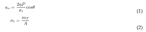
where a_o is the acceleration of sail tangential to the orbit, P is the magnitude of the solar radiation pressure (4.56X10⁻⁶Nm⁻²) exerted on a perfectly absorbing surface at a distance 1 AU. The sail efficiency η = 0.85, is a function of both the optical properties of the sail film and the sail shape due to billowing and wrinkling. σ_t is the total solar sail m_t as the total mass and A is the sail area. θ is the yaw angle of the sail normal relative to the Sun-sail line. Sails center on use of commercially available 7.5µm kapton film with a projected sail assembly loading of order 30gm⁻²- using this for different specifications of sail areas we can calculate the mass of the sail. To measure the efficiency of the sail, we can us the property of specific impulse I_sp of the sail. Since solar sails do not expel reaction mass the conventional definition of specific impulse is in appropriate. However for a finite mission duration, only a finite total impulse will be delivered by the solar sail. Infinite specific impulse is only available for infinite mission duration. In order to circumvent this difficulty with the conventional definition of the specific impulse, an specific impulse will be defined as the total impulse delivered per unit weight of the propulsion system.

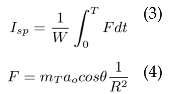
where F is the thrust delivered for mission duration T and W is the weight of the propulsion for a solar sail of mass m_T and the characteristic acceleration a_o at solar distance R (AU). As flux radiant intensity is directly proportional to the force F_µ we will consider the Force F_µ as the flux radiant intensity at the specific distance R (AU) from the sun. a_o just accounts for the prograde and retrograde velocity vectors, but in reality there are many other forces into consideration (primarily the radial and normal vectors).

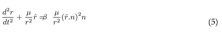
where r is the position vector of the sail with respect to the sun, with ˆr the associated unit vector. The product of the gravitational constant and the mass of the sun is defined by µ. For an ideal sail, the thrust vector is aligned along the sail unit normal vector n, with the sail pitch angle θ, defined as the angle between the sail normal and the radius unit vector such that cosθ = (r.nˆ)

5. Orbital Dynamics

Since we’ve looked into the model governing the whole system, we will be viewing a specific part of the system - orbital dynamics. The main factors that help us consider a set of orbital configurations is the time, distance, and ∆V of the orbit. We would require a set of equations that help us calculate these variables.

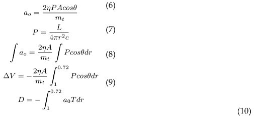
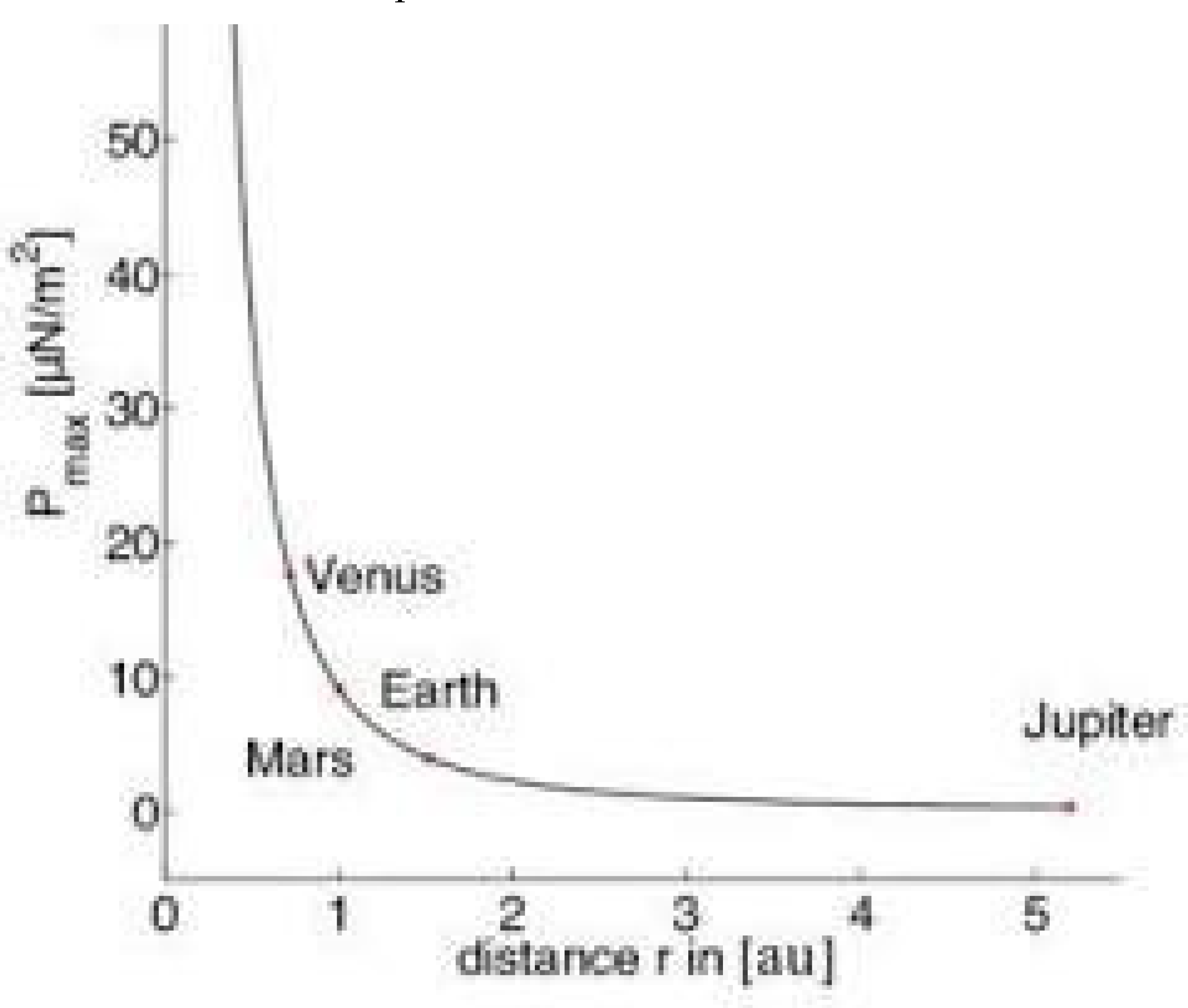
This set of equations describes how we can arrive at a numerical solution for the distance D, the time taken to reach the target, T where ^R a₀ is given by the graph of P against r, where r distance of the spacecraft from the sun. L is the luminosity of the sun and c is the speed of light in free space.

During the transfer, we must consider the blind spots when the resultant vector is the prograde vector because the photons are exposed to the back of the sail relative to the prograde vector. This happens when the relative θ is between 90 and 180. We can calculate the distance traveled around that arc the time it took to travel that particular distance.

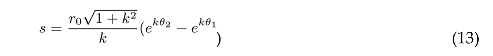
Plug in

r = r0ekθ

(12)

where k = −tanα, r₀ is 1 AU and θ is the angle relative to the start position.

We can figure out the amount of time it takes to travel the distance can be given by

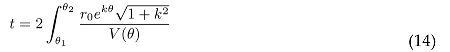
where V (θ) can be written as

V (θ) = 1.12 ∗ 10⁴ + ∆V

(15)

where the constant is the escape velocity of Earth Numerically the answer for s would come out to 0.48 AU and 6415921 s for t which is approximately 74 days. Assuming that it takes 1.5 of the spiral to reach the destination, it would result in the blind spot to be of 222 days throughout the course. To figure out the exact start position of Venus for the most optimum requirements we can use

This equation defines the starting position i.e the angle between the Earth-sun-Venus during the transfer window. T_course is the duration of the journey, 146 is time of course of a normal Hohmann transfer to Venus when the angle between the Earth-sun-Venus is 60.

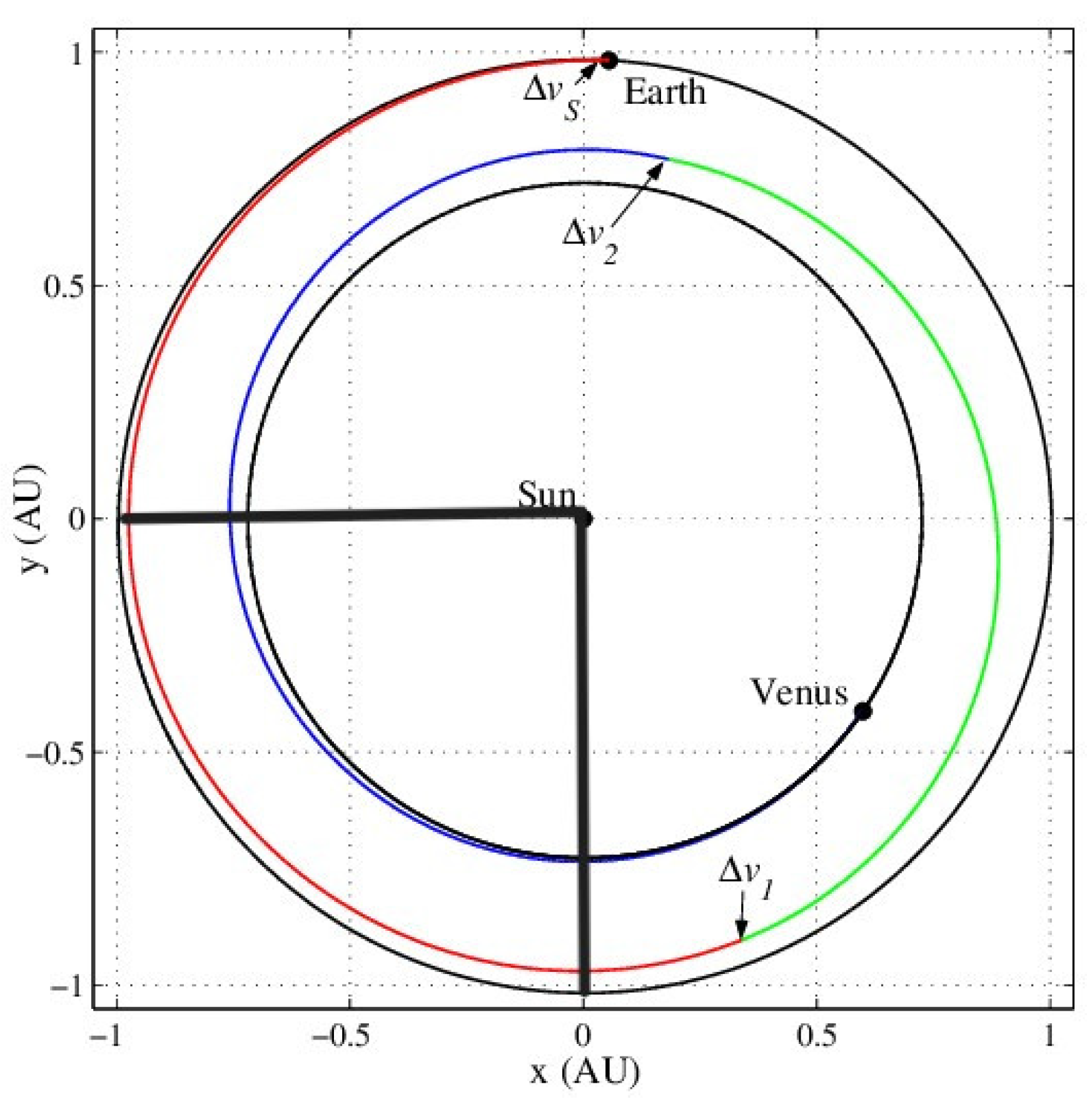
Figure 1. Logarithmic orbit to Venus.

Figure 1. Logarithmic orbit to Venus.

6. Why prefer Coplanar orbits in the XY Plane

If you can visualize a coplanar orbit in the XY plane, we can conclude that the early stages of motion is deceleration because of the angle made between the sunline and the sail, which is ideal because the resultant should be in the retrograde direction. The same representation in the XZ plane would also lead to deceleration in the early stages only if the angle between the sunline and normal is quite huge, but then it surpasses the calculated optimum angle. Moreover, the extreme angle between the sunline and the sail would lead to small changes in the radial vectors and massive changes in the normal vectors leading to deviation from the course.

7. Data Analyzation

The data recorded show the time, ∆ V, eccentricity, and each optimum angle for every iteration of a burn. To reach a valid conclusion on which iteration is the most optimum we can come up with a constant of efficiency or K_Eff. This would be the ∆V multiplied by the time multiplied by the optimum angle. The minimum answer to K_Eff would suggest that the least amount of time with least amount of ∆V is taken to reach the destination with a small deviation in the AoA with respect to the sunline which suggest the minimum amount of deviation from the original course. The 30 degrees added is to make sure that the sail is exposed to enough photons so that enough thrust is being produced. Each time measurement is multiplied by a factor K to incorporate the additional time it takes to reach the target since the thrust produced is minimal and there are many different combinations for the logarithmic spiral for every iteration. Each factor is multiplied by K because of the probability of getting a intercept with the Venus SOI is same for all eccentricities if we assume the SOI to be spherical and uniform on all sides.

8. Conclusion

The highlighted row shows the iteration with the most efficient solution which means it has the least numeric value for the constant of efficiency, K_Eff. This iteration was on the lower side of magnitude of numeric solutions of ∆V, was below the median for the field, Time. Major reasons why this solution is the most efficient is because it follows a coplanar orbit in the XY plane and is the closest to the inclination of Venus at 2.4 thus saving ∆V usage in normal vectors. We can also theoretically conclude that most efficient transfers are those whose orbital inclination are the closest to the targets orbital inclination. For this particular iteration

Missions with targets at high orbital inclination should be carried out in coplanar orbit in the XZ because of higher exposure time to photons in the direction where the photons give a resultant in the retrograde vector. Coplanar orbit in the XZ provide trajectories where the sail is more further away from planets and bodies during cruise which minimizes perturbations due to laws of Principia and Keplar’s law of motion.

Figure 2.

Figure 2.

Figure 3.

Figure 3.

References

- Pini Gurfil, [2006], Modern Astrodynamics, Israel, Elsevier.
- Topputo, Francesco and Vasile, Massimiliano, [2004], Interplanetary and lunar transfers using libration points, Italy, Research Gate.
Disclaimer/Publisher’s Note: The statements, opinions and data contained in all publications are solely those of the individual author(s) and contributor(s) and not of MDPI and/or the editor(s). MDPI and/or the editor(s) disclaim responsibility for any injury to people or property resulting from any ideas, methods, instructions or products referred to in the content. |
© 2025 by the authors. Licensee MDPI, Basel, Switzerland. This article is an open access article distributed under the terms and conditions of the Creative Commons Attribution (CC BY) license (http://creativecommons.org/licenses/by/4.0/).
Copyright: This open access article is published under a Creative Commons CC BY 4.0 license, which permit the free download, distribution, and reuse, provided that the author and preprint are cited in any reuse.