
Submitted:
12 June 2025
Posted:
13 June 2025
You are already at the latest version
Abstract
This research presents a comprehensive trustworthy machine learning framework for early diabetes detection, addressing critical gaps in reliability, interpretability, and fairness in clinical AI systems. The study integrates causal inference, modern ensemble methods (LightGBM, XGBoost-DART, HistGBM), and TabNet for tabular deep learning to enhance predictive performance while ensuring transparency. A novel Causal-guided Stacking Classifier (CGSC) is introduced, utilizing LightGBM as a meta-learner trained on causally relevant features identified through Causal Forests. The framework emphasizes interpretability through SHAP-based global and local explanations and leverages TabNet’s intrinsic attention mechanism for feature-level insights. Counterfactual reasoning (DiCE) enables personalized risk mitigation strategies by identifying minimal feature changes to alter predictions. To promote fairness, gender is excluded as a direct feature, reducing demographic bias. Experimental results demonstrate robust performance: CGSC achieves the highest recall (0.81), critical for early warning systems, while TabNet attains superior precision (0.79). Uncertainty quantification reveals stable F1-scores (0.73 ± 0.03) across ensemble models. Key causal drivers include general health (ATE = 0.1392) and cardiovascular factors, while counterintuitive findings like alcohol consumption’s negative association (ATE = -0.1875) warrant further investigation. The framework’s emphasis on causal feature selection, model transparency, and actionable explanations aligns with healthcare requirements for trustworthy AI, offering a reproducible solution for diabetes risk stratification with potential clinical applicability. All experiments are fully reproducible, with resources available at the GitHub repository.
Keywords:
Causal Inference
; Trustworthy ML
; Tabular Deep Learning
; Diabetes Early Warning
1. Introduction
Diabetes mellitus stands as one of the most pressing global health challenges of the 21st century, with a rapidly increasing prevalence and substantial economic impact. In 2021, approximately 537 million adults were living with diabetes worldwide, a figure expected to rise to 643 million by 2030 and 783 million by 2045 [1]. Recent estimates suggest that nearly 1 in 9 adults globally are now affected, underscoring an escalating health crisis that disproportionately burdens low- and middle-income countries [2]. Beyond individual morbidity, diabetes contributes heavily to healthcare expenditures, with global costs exceeding USD 966 billion annually [3].
Timely detection and early warning are vital, as delayed diagnosis often results in severe long-term complications, including cardiovascular disease, neuropathy, retinopathy, and renal failure [4]. However, early-stage diabetes is frequently asymptomatic or presents with nonspecific symptoms, making proactive identification particularly challenging [5]. Current screening methods typically rely on threshold-based biomarkers such as fasting plasma glucose, oral glucose tolerance tests (OGTT), and HbA1c levels [7]. While clinically validated, these markers are inherently binary and fail to reflect the continuous and multifactorial nature of glucose dysregulation [8]. Additionally, these measures are susceptible to biological variability and external factors such as stress, medications, and ethnicity, which can introduce diagnostic errors [9].
Traditional diagnostic approaches also tend to assess risk factors in isolation, such as BMI, blood pressure, lipid levels, and family history, without capturing their complex interdependencies. This siloed perspective limits the capacity to detect subtle, early-stage pathophysiological changes or to tailor prevention strategies to individual profiles [10]. While multivariable risk scores like the Finnish Diabetes Risk Score (FINDRISC) offer some improvement, their predictive accuracy remains modest across heterogeneous populations [11].
These limitations highlight the urgent need for adaptable, data-driven screening systems capable of integrating diverse risk indicators and capturing individualized patterns of disease onset. In particular, machine learning–driven early warning models, augmented with counterfactual reasoning, offer the potential to go beyond prediction by providing actionable, personalized preventive insights before clinical symptoms manifest.
The global expansion of digital health records, biometric data, and health-related behavioral tracking offers new opportunities to enhance disease detection. In this data-rich context, machine learning (ML) has emerged as a promising avenue to uncover hidden patterns and predictive markers in large-scale tabular data [6]. The increasing digitization of healthcare, generally due to the widespread availability of electronic health records (EHRs) and biometric data, has opened a path for machine learning (ML) to play a transformative role in disease diagnosis, and so do in risk stratification. In the context of diabetes, ML models provide distinct advantages over traditional diagnostic systems by enabling the discovery of complex and nonlinear relationships among numerous clinical and behavioral variables. Algorithms like decision trees, support vector machines, and ensemble methods such as random forests have demonstrated improved accuracy in identifying undiagnosed diabetes or predicting future onset compared to conventional models [12]. These predictive techniques are particularly well-suited for tabular medical data that allows for the inclusion of a wide array of risk factors such as age, BMI, blood pressure, lipid profiles, and lifestyle indicators without the need for pre-specified interactions [13]. Furthermore, ML frameworks can be continuously updated as new data becomes available. Thus, it supports dynamic learning and adaptation to evolving population health trends. Nevertheless, even after having all these advantages, widespread clinical adoption of ML remains constrained by critical challenges in interpretability, fairness, and reliability that are essential in healthcare contexts where transparency and trust are necessary for clinical decision-making. A big step toward enabling more ethical, scalable, and personalized early detection systems is to address these issues.
Machine learning systems are increasingly integrated into clinical workflows, and hence the demand for trustworthy AI systems that are not only accurate but also reliable, fair, and interpretable is growing significantly. In healthcare, the stakes are particularly high because predictions directly impact patient outcomes, influence clinical decisions, and affect resource allocation. Trustworthiness in this domain encompasses several critical dimensions, including but not limited to robustness to data shifts, transparency of model decisions, mitigation of bias, and accountability for outcomes [16]. A foundational role in ensuring trust is played by interpretability as well. Clinicians must be able to understand why a model arrives at a particular prediction, especially when it contradicts clinical intuition. Black-box models, even when accurate, are often met with resistance in healthcare due to their lack of explanatory power [17]. Moreover, fairness and bias mitigation are essential, as healthcare datasets often reflect underlying social inequities. If these biases remain unchecked, they can propagate through algorithms and disproportionately affect vulnerable populations. As regulatory frameworks such as the European Union’s AI Act and U.S. FDA guidelines evolve, healthcare ML systems will increasingly need to demonstrate transparency, equity, and robustness in real-world deployment. The development of trustworthy AI systems is thus not solely a technical challenge but a multidimensional task intersecting ethics, policy, and clinical practice.
Furthermore, despite advances in machine learning for diabetes detection, most existing studies continue to focus narrowly on predictive accuracy, leaving several critical dimensions unaddressed. Many models rely on correlational features derived from statistical associations, which may not generalize across populations or yield clinically meaningful insights. Without a causal grounding, such models are limited in their ability to support reasoning about interventions or to explain why a particular prediction occurs. Interpretability remains underdeveloped in ensemble and deep learning models. While these architectures excel at capturing complex patterns, they often obscure the decision process, making it difficult for clinicians to trust or act upon individual predictions. Even when interpretability tools are applied, they rarely connect insights to potential interventions. Another major shortfall is the limited use of counterfactual reasoning. Existing ML systems almost never explore what-if scenarios to suggest preventive pathways or minimal changes needed to reduce risk. This absence restricts their role from passive prediction to active clinical decision support. Additionally, fairness considerations are frequently sidelined; many studies fail to evaluate model performance across demographic subgroups or to mitigate bias in feature selection and outcome prediction. Ultimately, few frameworks holistically integrate causality, interpretability, fairness, and actionable counterfactuals, leaving a significant gap in the development of clinically trustworthy AI systems.
Therefore, this research aims to address the aforementioned gaps by developing a comprehensive and trustworthy machine learning framework for early diabetes detection. The major contributions of this work are summarized as follows:
- Proposed a novel Causal-guided Stacking Classifier (CGSC) that synergistically integrates causal feature selection, ensemble learning, and interpretability to enhance model trustworthiness and clinical relevance.
- Utilized Causal Forests for robust feature selection, identifying stable and causally relevant predictors that improve generalizability and resilience to distributional shifts.
- Experimentally applied the modern and underutilized tabular deep learning architecture, TabNet, to leverage its interpretability and performance advantages in structured healthcare data.
- Designed and implemented counterfactual reasoning mechanisms to provide actionable, individualized recommendations by simulating preventive interventions at the feature level for high-risk patients.
- Conducted comprehensive uncertainty analysis by evaluating the distribution of F1-scores across multiple training iterations, thereby assessing model reliability and prediction stability.
- Employed SHAP-based feature attribution for both global and local interpretability, complemented by TabNet’s attention mechanism to visualize feature importance at the individual prediction level, facilitating transparency and clinician trust.
Literature Review
Ghosh and Argal [18] proposed a robust ensemble learning framework for diabetes onset prediction by integrating exploratory data analysis (EDA) with multiple classifiers, including Random Forest, Gradient Boosting, and XGBoost. Their methodology emphasized data preprocessing and correlation mapping to uncover hidden factors influencing diabetes risk. Their ensemble approach achieved a peak accuracy of 89.6% on the Pima Indian Diabetes dataset, outperforming traditional single classifiers. Importantly, the study utilized SHAP values and feature importance scores to enhance interpretability and ensure transparency in model predictions, highlighting the synergy between pre-modeling insights and ensemble learning in medical diagnostics.
Kirubakaran et al. [19] introduced a fuzzy support vector regression (FSVR) model tailored for progressive diabetes detection. Aiming to mitigate high false-positive rates in binary classifiers, the authors incorporated fuzzy logic to effectively handle uncertainty in patient data. The FSVR model achieved an accuracy of 91.2% and demonstrated robustness to noisy features on a real-world clinical dataset. Its interpretable decision boundaries render it particularly suitable for clinical settings where explainability is essential. The authors recommend future integration of hybrid optimization techniques to enhance scalability and performance.
Alkhaldi et al. [20] investigated the predictive potential of biochemical markers such as liver enzymes (ALT, AST) and BMI for early type 2 diabetes diagnosis using gradient boosting and logistic regression. Their study, based on a dataset of over 5,000 patients, achieved an AUC-ROC of 0.93. The identification of ALT as a more significant predictor than BMI challenged conventional clinical assumptions. With SHAP-based feature attribution, their model preserved high sensitivity across diverse demographic groups, offering a cost-effective and non-invasive diagnostic pathway.
Meng et al. [21] proposed a deep learning-based, non-invasive diagnostic method for diabetic kidney disease (DKD) using retinal fundus images. By employing convolutional neural networks (CNNs), the model achieved an AUC above 0.95 in distinguishing DKD from isolated diabetic nephropathy. This work pioneers a diagnostic paradigm that leverages retinal imaging as a proxy for renal health, enabling earlier detection while eliminating the need for invasive procedures such as biopsies.
Sushith et al. [22] developed a hybrid deep learning model combining CNNs and recurrent neural networks (RNNs) to detect early signs of diabetic retinopathy. The CNN component captured spatial features, while the RNN tracked temporal disease progression. Their model outperformed standalone CNNs, achieving a 96.1% accuracy and demonstrating high specificity—qualities that are vital for reliable screening. This study underscores the necessity of modeling time-dependent features in chronic disease progression.
Xiao et al. [23] introduced an interpretable machine learning framework guided by clinically relevant biomarkers for diabetes diagnosis. Employing logistic regression and decision trees, the study focused on transparent feature selection and interpretability. Trained on a Chinese cohort, the model achieved an 87% accuracy using biomarkers such as HbA1c, insulin, and triglycerides. SHAP-based explanations and clinician validation reinforced the model’s trustworthiness and clinical applicability.
Wang et al. [24] implemented a Single Shot Multibox Detector (SSD)-based architecture to classify stages of diabetic retinopathy from high-resolution retinal images. Compared to conventional CNNs, SSD achieved over 93% accuracy and facilitated real-time lesion detection. Its balance of speed and accuracy makes it well-suited for deployment in low-resource settings where rapid and accurate diagnostics are crucial.
Gupta et al. [25] introduced a Quantum Transfer Learning (QTL) approach for diabetic retinopathy classification. Combining ResNet-based feature extraction with a quantum-enhanced classifier, the model outperformed classical deep learning baselines in precision and inference time, achieving an accuracy of 95.3%. The study highlights the emerging role of quantum AI in advancing medical diagnostics through parallelism and energy-efficient computation.
Ge et al. [26] tackled the early prediction of low muscle mass (LMM) in diabetic and obese patients using a supervised random forest model. Incorporating clinical, metabolic, and demographic features, the model attained an AUC of 0.88 and identified serum albumin, body fat percentage, and HbA1c as key predictors. This work draws attention to an often-overlooked comorbidity and presents actionable strategies for early clinical intervention.
The current literature places significant emphasis on the diagnosis and interpretability of diabetes-related conditions. However, relatively few studies have explored proactive early-warning systems that require minimal or no clinical intervention. Such systems, especially when enhanced with counterfactual reasoning and causal inference-based feature selection, have the potential to offer personalized and preventive recommendations. Moreover, while interpretability methods like SHAP are increasingly adopted, the field still lacks robust frameworks that combine transparency, reliability, and user trust—core pillars of trustworthy machine learning. This research aims to bridge these gaps by focusing on the development of models that not only perform well but also align with the principles of trustworthy AI in healthcare: interpretability, fairness, robustness, and user-aligned explanations.
2. Methodology
This section describes the workflow of how the research is conducted. GitHub repository of this research contains every file and resource that are necessary to replicate this study in future. [27]
2.1. Dataset Information
A dataset from Kaggle, entitled “diabetes_data” uploaded by Prosper Chuks is utilized for modeling purposes. The dataset has 70692 instances, and 18 columns with 17 features and a target variable. The features contain internal and external physical attributes, lifestyle choices, and demographic information about each individual, whereas the target column contains whether the individual has diabetes or not. The dataset contains the following columns: Age, Sex, HighChol, CholCheck, BMI, Smoker, HeartDiseaseorAttack, PhysActivity, Fruits, Veggies, HvyAlcoholConsump, GenHlth, MentHlth, PhysHlth, DiffWalk, Stroke, HighBP, and Diabetes. Definitions of each column and the values they take are given in Table 1. It is noticable that, knowing the information of these variables does not require any clinical intervention. Therefore, developing an early warning system for diabetes utilizing machine learning algorithm is possible with this dataset.
2.2. Data Preprocessing
The dataset is free from missing values and contains no duplicates. Additionally, all features are already numeric, eliminating the need for encoding categorical variables. The target variable was originally of float data type, which was subsequently cast to an integer to simplify model training and evaluation. To minimize the risk of demographic bias, the “Sex” attribute was removed. While this step eliminates direct gender-based influence, it does not fully prevent the model from learning latent or proxy bias. Such indirect biases can persist through correlated features and require more sophisticated mitigation strategies, such as proxy variable testing, sample reweighting, adversarial debiasing, or fairness-constrained optimization, which fall outside the scope of this study.
Furthermore, the dataset exhibits signs of heteroskedasticity, as illustrated in Figure 1. For visualization, the standard deviation of each feature was plotted instead of variance. This choice was made because several features span a wide numerical range, causing their variances to dominate the plot and obscure meaningful comparison across features with smaller magnitudes. Using standard deviation ensures a more interpretable and balanced visualization across all features.
For parametric models like Logistic Regression or Neural Networks, heteroskedasticity causes a problem by emphasizing more on the features having higher range of values. Conversely, for non-parametric models like NGBoost or any other ensemble models, it does not create any problem as these models learn internal data patterns with decision rules. Therefore, the data is not scaled at this stage. However, during the training of TabNet- which is a tabular neural network, the data was scaled using z-score standardization from scikit-learn’s StandardScaler().
Figure 2 presents a visual comparison between diabetes and non-diabetes instances in the dataset based on their clustering behavior. To enable this, Principal Component Analysis (PCA) was employed to reduce the original high-dimensional feature space into two principal components. These two components capture the maximum variance in the data and serve as the new feature axes for visualization. The resulting 2D scatter plot distinctly shows how individuals with and without diabetes are distributed in the transformed space, thereby offering insights into potential separability of the classes using machine learning methods.
A correlation heatmap of the features is shown in Figure 3. It is shown that several low to moderate correlations between the features exist. For example, “GenHlth” and “PhysHlth” are moderately correlated with a coefficient of 0.55. Worsening of “GenHlth” is also slightly associated with heart diseases or attack with a correlation coefficient of 0.28.
Figure 4 shows that there is no class imbalance in the dataset.
Class imbalance affects negatively on the learning ability of machine learning models. In cases of severe class imbalance, the models prioritize major classes to learn internal data patterns, which lead to poor generalization and performance. Fortunately, dealing with such scenarios is not required in this research.
2.3. Model Selection
As mentioned before, three ensemble models are selected for modeling purposes. These models are XGBoost Dart, Light Gradient Boosting Machine (LGBM), and Histogram-based Gradient Boosting Classifier (HistGB). The hyperparameters of these models are tuned with Bayesian Optimization for this task of diabetes diagnosis. Also, a stacked ensemble consisting of the mentioned three ensembles and LGBM as meta-estimator is utilized. This stacked ensemble is trained on causal features. Tabular neural model TabNet is experimentally used to analyze how it performs on diabetes prediction. Uncertainty quantification of the ensemble and causal-guided model is provided. The most optimal model’s SHAP interpretation alongside diverse counterfactual explanations (DiCE) is incorporated as well. A brief description of the models is given below.
2.4. Light Gradient Boosting Machine (LightGBM)
LightGBM is a highly efficient gradient boosting framework based on decision trees, developed by Microsoft. It is designed to be both faster and more memory-efficient than traditional boosting algorithms due to two key techniques known as Gradient-based One-Side Sampling (GOSS) and Exclusive Feature Bundling (EFB).
LightGBM constructs trees leaf-wise rather than level-wise. The algorithm selects the leaf with the maximum loss reduction at each step. This leads to faster convergence and often better accuracy on tabular datasets. The objective is to minimize a differentiable loss function using gradient boosting:
The ensemble is trained sequentially, where weak learner attempts to minimize the residual errors of the previous learners:
LightGBM is selected for this work due to its strong performance on tabular data, scalability to large datasets, and compatibility with interpretability tools such as SHAP.
2.5. XGBoost DART (Dropout Additive Regression Trees)
XGBoost DART is another ensemble model and a variant of the eXtreme Gradient Boosting (XGBoost) algorithm that incorporates dropout techniques inspired by neural networks in order to prevent overfitting. DART randomly drops a subset of trees while training a new tree, instead of using all the trees in the ensemble at each iteration:
Here, D represents the set of dropped trees, and is the newly learned regression tree that corrects the bias in the current prediction. The model introduces randomness and regularization into the boosting process to enhance generalization on datasets with potential overfitting. There, XGBoost DART was chosen due to its strong regularization ability, and strong track record in machine learning competitions.
2.6. Histogram-Based Gradient Boosting Machine (HistGBM)
Histogram-Based Gradient Boosting is another variant of traditional gradient boosting decision trees (GBDT), where continuous features are first bucketed into discrete bins (histograms). This reduces memory usage and speeds up training by allowing for histogram-based split finding:
Using histogram-based discretization, the model only searches for splits among a fixed number of bins k, that accelerates computation without sacrificing much accuracy. HistGBM is selected for this task as an faster alternative of previously mentioned gradient boosting models. HistGB usually has decent computational efficiency and competitive performance, especially when working with medium-sized clinical datasets. It is also supported natively by the scikit-learn library, making it easily integrable within cross-validation and pipeline frameworks.
2.7. TabNet: Deep Learning with Sparse Attention for Tabular Data
TabNet is a newborn deep neural network architecture tailored for tabular datasets that combines the high performance of deep learning with interpretability, traditionally seen in decision trees. Unlike conventional feed-forward neural networks, TabNet uses a sequential attention mechanism that enables the model to learn which features to focus on at each decision step. This allows for both local interpretability (why the model made a specific decision) and global interpretability (which features are generally important).
Model Architecture
TabNet operates in multiple decision steps. At each step t, a feature transformer network processes the input features, and an attention mask is generated to determine which features should be emphasized in the current decision step. The overall prediction is formed by aggregating outputs across all decision steps:
where: - x is the input feature vector, - is the sparse attention mask at decision step t, - ⊙ denotes element-wise multiplication (masking), - is the transformation block producing output at step t.
Sparse Attention and Interpretability
A key novelty of TabNet is its sparse attention mechanism, which enforces that only a subset of input features contribute at each decision step. This is achieved using a learned softmax-based mask over the features with a sparsity-inducing regularization term added to the loss function:
This regularization encourages attention distributions to be sparse, which turns the model more interpretable by focusing only on the most relevant features. The interpretability can be visualized by aggregating the learned masks across decision steps for each sample (local) or across all samples (global). This makes TabNet particularly suitable for medical diagnosis, where understanding why a prediction was made is critical.
Mathematically, the interpretability in TabNet is achieved through the use of a sparse attentive mechanism in its decision steps. At each decision step i, the model applies a learned feature mask over the input feature vector x, where:
Here, is the learnable projection at decision step i, and the Sparsemax activation ensures that the resulting mask is sparse, i.e., it selects only a small subset of features for consideration at each step. This sparse masking enables the model to focus on the most relevant features per sample and per decision step, leading to both efficient learning and built-in interpretability.
The global feature importance shown as plot is derived by aggregating these masks across all decision steps and across all training samples. If we denote the aggregated importance of feature j as:
where T is the number of decision steps, and N is the total number of samples, we get a global importance score for each feature. These values reflect how often and how strongly each feature was attended to during the training process.
TabNet is chosen for this study due to its unique combination of:
- Deep learning power: Capable of learning complex nonlinear interactions in tabular clinical data.
- Built-in interpretability: Sparse attention directly shows which features influenced the model decision.
- No preprocessing: Unlike tree-based models, TabNet handles raw numeric and categorical data without the need for heavy preprocessing.
- Trustworthiness: Ideal for high-stakes healthcare settings where interpretability and decision transparency are necessary.
Despite having these advantages, TabNet is extremely underutilizied in medical domain. Hence, an experimental run and performance evaluation of TabNet on the diabetes data is presented in this paper to align with the recent technological advancements. Moreover, in this work, TabNet’s feature masks are analyzed to understand which features were most salient in predicting diabetes for each individual, as well as globally across the cohort. This forms a critical part of the proposed framework’s interpretability pipeline.
2.8. Causal Inference-Based Feature Selection
With an attempt to identify features with a stable and causal impact on the target variable (Diabetes), the Causal Forest model from the econML library [14] is employed. Each candidate feature was individually treated as a treatment variable T, and its effect on the binary target Y (presence of diabetes) was estimated using Causal Forests.
The Causal Forest model is based on the potential outcomes framework [15], which assumes that for each individual i, there exists a potential outcome under treatment level t. The individual treatment effect (ITE) is defined as:
Since it is not possible to observe both potential outcomes for the same individual,the Average Treatment Effect (ATE) is estimated, which is the expectation over the population:
For continuous treatments, the ATE generalizes to estimating the expected change in outcome per unit change in treatment, while controlling for confounding variables X. Formally:
To adjust for confounding bias, treatment-specific confounders through a two-step data-driven process are identified:
- For each candidate treatment variable , a Random Forest model to predict using all other features excluding the target Y and itself is trained.
- From the trained model, the top features that cumulatively explained 80% of the total feature importance are selected, denoted by the set . These were treated as the confounders for estimating the effect of on Y.
Using the Causal Forest DML estimator, the ATE is estimated for each treatment variable while adjusting for its corresponding confounders . Treatment variables that showed an average treatment effect of at least 1% (i.e., ) were considered causally relevant. These features were then selected for inclusion in the stacked ensemble model. The entire process is outlined in Algorithm 1.
| Algorithm 1:Causal Feature Selection with Causal Forests |
|
Require: Dataset with features and binary target Y Ensure: Selected set of causal features
|
This process makes sure that only features with a causal and stable relationship with the target are used for downstream predictive modeling. This can lead to an improvement in both interpretability and generalizability.
3. Results and Discussion
This section provides detailed analysis on model performance, uncertainty, interpretability, and counterfactuals.
3.1. Model Evaluation
Table 2 shows the performance comparison of the five models—XGBoost Dart, LightGBM, HistGB, TabNet, and the Causal-Guided Stacked Classifier (CGSC). It reveals distinct strengths and weaknesses across key performance metrics. XGBoost Dart demonstrates robust performance with a precision of 0.76, recall of 0.80, and an F1-score of 0.78, denoting a well-balanced trade-off between identifying true positives and minimizing false positives. The accuracy of the model is 0.78 and AUC is 0.84, which further underscore its reliability as a general-purpose classifier. LightGBM, while exhibiting a slightly lower precision (0.71) and recall (0.76), achieves an exceptional AUC of 0.97, suggesting superior discriminative power in distinguishing between classes, albeit with a marginally lower accuracy of 0.72. HistGB shows moderate performance across all metrics, with precision, recall, and F1-score each hovering around 0.72–0.73, alongside an accuracy of 0.72 and an AUC of 0.78. The ROC-AUC curve of the ensemble models is shown in Figure 5.
TabNet stands out with the highest precision (0.79) among the models. It reflects the model’s ability to minimize false positives, though its recall of 0.73 is comparatively lower, that indicates a potential shortfall in capturing all positive instances. Its F1-score of 0.76 and accuracy of 0.77 combined with a strong AUC of 0.86 suggest that is well-suited for applications where precision is paramount. The CGSC model, which integrates Logistic Regression and kNN as base learners with LightGBM as a meta-learner, achieves the highest recall (0.81) but the lowest precision (0.70). This inverse relationship highlights its tendency to prioritize identifying true positives at the cost of increased false positives, which turns it particularly useful in domains like early disease diagnosis where missing a positive case is more detrimental than occasional false alarms. Its F1-score of 0.75 and accuracy of 0.73 are competitive, while its AUC of 0.80 indicates reasonable discriminative capability. Figure 6 illustrates the ROC-AUC curve of these two models.
For an early warning diabetes prediction task using non-clinical features, the optimal model should prioritize high recall, good precision, and strong AUC. So, in terms of recall, CGSC is the best model, where for a balanced performance, TabNet and XGBoost shines. However, early warning systems benefit most from high recall as missed cases can lead to preventable complications. CGSC’s recall-driven performance aligns best with this goal, while XGBoost provides a safer middle ground if precision cannot be sacrificed entirely.
In the uncertainty plots presented in Figure 7, each of the four models—CGSC, XGBoost DART, HistGB, and LGBM—was evaluated over 100 runs in terms of their F1-score variability.
The CGSC model shows a relatively narrow F1-score range of approximately 0.70 to 0.76. Its average performance seems to cluster around 0.735 to 0.74, and although there are a few dips, they are not frequent or severe. This reflects a stable and consistent behavior across repeated executions.
On the other hand, the XGBoost DART model, reaches higher F1-score peaks, ranging from about 0.69 to 0.82, with its mean likely around 0.76 to 0.77. However, the model also exhibits significant fluctuations, that shows frequent drops in performance alongside its high scores. This result suggests a higher variance in behavior which could lead to unpredictable outcomes if not controlled or averaged out.
The HistGB model demonstrates the most erratic performance of the four. Its F1-scores fluctuate between approximately 0.67 and 0.81, with a presumed average close to 0.735. This model suffers from frequent sharp dips and spikes that denotes considerable instability and variance across runs. Such unpredictability could make it less desirable for applications like diabetes diagnosis that requires reliability.
Finally, the LGBM model operates within an F1-score range of roughly 0.66 to 0.78. Its average seems to fall between 0.735 and 0.74, and although it displays performance swings, they are less extreme than those seen in HistGB. Nevertheless, its moderate-to-high variance indicates a certain level of unreliability, albeit to a lesser extent.
Therefore, CGSC emerges as the best option for consistency and robustness in terms of overall preference, with the most stable F1-score across the 100 runs. It performs reliably and avoids dramatic fluctuations, making it well-suited for scenarios where predictability is crucial. Conversely, XGBoost DART delivers the highest individual F1-score performances and could be the optimal choice when maximizing peak accuracy is a priority, provided that its higher uncertainty is managed—potentially through ensemble methods or additional tuning. HistGB stands out as the least stable model, with its highly volatile performance making it a less favorable choice in most practical settings. LGBM sits between the extremes by showing moderate reliability but not excelling significantly in either consistency or peak performance.
3.2. XGBoost DART Global Interpretability
In order to enhance the transparency and trustworthiness of the diabetes prediction framework, SHAP (SHapley Additive exPlanations) is utilized to interpret the XGBoost DART model globally and locally. SHAP values, grounded in cooperative game theory, attribute a contribution value to each feature by estimating how much each one shifts the model’s output from the base value.
The SHAP summary plot in Figure 8 visualizes both the importance and direction of influence of each feature. The horizontal axis represents the SHAP value, which denotes the impact of each feature on the model’s prediction. Features are ordered vertically based on their overall contribution across the dataset.
Each point on the plot corresponds to an individual prediction, where the color represents the feature value (red for high, blue for low). A positive SHAP value implies that the feature increases the probability of predicting diabetes, whereas a negative value denotes the opposite.
As observed, GenHlth (General Health), BMI, Age, and HighBP (High Blood Pressure) are the most influential features. Individuals with poor general health (high feature value in red) tend to have positive SHAP values. It explains that they are more likely to be predicted as diabetic. Similarly, higher BMI and older age also contribute positively to the model’s prediction. Conversely, higher levels of physical activity (PhysActivity) and lower cholesterol levels (HighChol) are associated with negative SHAP values. These features act as protective factors.
The model effectively captures non-linear dependencies and feature interactions. For example, even though high blood pressure generally contributes positively to diabetes risk, there are low-value instances (in blue) that occasionally have a small positive SHAP value that reflects contextual interactions with other features.
This global SHAP interpretation validates the clinical plausibility of the model’s reasoning and identifies the most salient risk factors for diabetes in the dataset. It also ensures that the model decisions align with domain knowledge, which strengthens its credibility in real-world deployment. However, real-world deployment is beyond the scope of the research for now.
3.3. XGBoost Dart Local Interpretability
The model’s decision-making process for individual predictions using local SHAP explanations is also investigated to complement the global interpretability analysis. Figure 9 shows a waterfall plot for a single instance that was classified as not diabetic (class 0) by the XGBoost DART model.
The SHAP framework decomposes the model output into a sum of contributions from each feature relative to the expected prediction. The expected value of the model output is . It represents the average model prediction across the dataset. For this specific individual, the final model prediction is , which strongly pushes the prediction towards the non-diabetic class.
Each bar in the waterfall plot corresponds to a feature’s SHAP value contribution. Blue bars indicate features that pushed the prediction lower (towards class 0), whereas red bars indicate features that pushed the prediction higher (towards class 1).
The most influential feature is BMI, which contributes to the model output, which suggests a relatively low BMI for this individual. This is followed by General Health (GenHlth), which adds another , it points to the fact that the person self-reported good general health. Age has a slight positive contribution of , denoting older age slightly increases the likelihood of diabetes, but not enough to override the strong negative contributions from other features.
Other negative contributors include HighBP (), HighChol (), and PhysActivity (), suggesting that the individual does not have high blood pressure or cholesterol and is physically active—all of which are consistent with a lower risk of diabetes. The remaining features such as Stroke, HeartDiseaseorAttack, and PhysHlth also have slight contributions.
This localized interpretation ensures transparency at the individual level that confirms the alignment of model’s prediction with clinical reasoning. It further enables trust in model deployment, especially in sensitive healthcare settings where individualized decisions matter.
Similarly, the local SHAP explanation illustrated in Figure 10 corresponds to an individual who was predicted as diabetic (class 1) by the XGBoost DART model. The model’s expected output is , whereas the final prediction for this instance is significantly higher, , indicating a high likelihood of diabetes.
The feature with the highest positive contribution is General Health (GenHlth), which adds to the prediction. This suggests the individual reported poor general health that is indeed a strong risk factor associated with diabetes. BMI also positively contributes that implies an elevated body mass index, another major risk indicator. Although Age contributes negatively (), as category 5 reflects a younger age, this is outweighed by the stronger positive contributions.
Additional features such as HighBP (), PhysActivity (), and PhysHlth () also pull the prediction higher. This insight suggests an association of limited physical activity or physical health issues with diabetes risk. Conversely, HighChol contributes negatively, it indicates that normal cholesterol somewhat mitigated the prediction, though not enough to change the final outcome.
This SHAP plot reaffirms the model’s decision in an interpretable manner, showcasing how combinations of risk factors (particularly poor general health and high BMI) drive a high-confidence diabetes prediction.
3.4. TabNet Global Interpretability
The bar chart provided in Figure 11 visualizes the global feature importance scores generated by TabNet. The x-axis represents the importance score which is a normalized value that sums to 1 across all features, and the y-axis lists the input features used in the model. The longer the bar, the more frequently or more significantly the feature was used in TabNet’s decision-making process.
From the plot, the feature GenHlth (General Health) has the highest importance score which explains that the model relies heavily on this feature when predicting the likelihood of diabetes. This makes sense in a healthcare context since general health status often correlates with chronic conditions like diabetes.
BMI and HighBP (high blood pressure) are also highly weighted, consistent with known risk factors for diabetes. On the other hand, features such as PhysActivity and MentHlth have very low importance scores. It implies that they contribute little to the predictive power for early warning of diabetes. The global feature importance in TabNet provides both an interpretable and theoretically grounded summary of which input features influence the model’s decisions. Fortunately, interpretability lead by the sparse attention mechanism is intrinsic to the model architecture and does not require post hoc explanations like SHAP or LIME. As a result, it is possible to directly trust the attribution scores to guide feature selection, model understanding, or communication of results to domain experts.
3.5. TabNet Local Interpretability
Figure 12 illustrates the local feature importance derived from a TabNet model when predicting an instance as diabetic (class 1). The horizontal bar plot displays the importance scores of each input feature. It mentions how significantly each feature contributed to the model’s decision for this particular individual.
From the plot, it is explicit that PhysHlth (Physical Health) is the most influential feature in the model’s prediction, with an importance score approaching 3.5. This suggests that the number of physically unhealthy days reported by the individual played a dominant role in classifying them as diabetic. The next most impactful features are BMI (Body Mass Index) and GenHlth (General Health), which denotes that higher body mass and poorer self-rated general health are also critical in determining diabetes presence for this subject.
Other features with notable contributions include Smoker and HighBP (High Blood Pressure), which align with known risk factors for diabetes. The variables HighChol, DiffWalk (Difficulty Walking), and MentHlth (Mental Health) show moderate influence, suggesting some relationship but to a lesser extent.
Features such as Age, CholCheck, PhysActivity, Fruits, Veggies, HvyAlcoholConsump, and HeartDiseaseorAttack contributed minimally in this individual case. These variables may be important at a population level, but their low scores here indicate limited relevance in the model’s specific decision for this person.
This analysis emphasizes the personalized interpretability provided by TabNet that adapts the contribution of features based on the unique characteristics of the individual case. It allows for more precise clinical insights and decision-making support.
On the other hand, Figure 13 illustrates the local feature importance scores generated by the TabNet model for an individual who was classified as not having diabetes. This interpretation allows us to examine which features contributed most significantly to the model’s prediction for this specific instance.
Among all features, GenHlth (General Health) holds the highest importance score by a considerable margin, indicating that the individual’s self-reported general health status played a dominant role in the model’s decision. The importance score for GenHlth exceeds 2.7, far surpassing that of any other feature, Which suggests that better perceived general health likely contributed to the classification as non-diabetic. Other features with moderate importance include HvyAlcoholConsump (Heavy Alcohol Consumption), Fruits (fruit intake), and BMI (Body Mass Index), have importance scores ranging approximately between 0.6 and 0.8. These features likely provided additional evidence supporting the non-diabetic classification, possibly by aligning with healthier lifestyle patterns or lower obesity risk. Additional contributions came from PhysHlth (Physical Health) and HeartDiseaseorAttack, though their influence was lower in magnitude. Interestingly, features such as HighBP (High Blood Pressure), Stroke, Smoker, and PhysActivity registered negligible or near-zero importance, pointing to the fact that they did not influence the model’s decision for this particular instance.
This localized explanation highlights TabNet’s ability to assign dynamic importance to features based on the specific characteristics of the input data. In this case, it shows a heavy reliance on self-reported health and lifestyle indicators over clinical history or demographic information when predicting the absence of diabetes.
3.6. Diverse Counterfactual Explanations
DiCE (Diverse Counterfactual Explanations) framework is employed to better understand the decision boundary of the predictive model. Figure 14 presents a counterfactual analysis where the goal was to identify minimal yet diverse feature changes that would alter the prediction of a given individual from non-diabetic (class 0) to diabetic (class 1).
The first row of the table corresponds to the original instance classified as non-diabetic. Notably, this individual has a low BMI of 20.0, does not suffer from high blood pressure, stroke, or walking difficulties, and reports excellent general health (GenHlth = 0.0, indicating "excellent"). The physical health burden (PhysHlth) is minimal, and lifestyle indicators such as PhysActivity and Fruits intake appear favorable.
The subsequent rows display counterfactual examples that lead to a prediction of diabetes (class 1) while keeping most features constant. Across all three counterfactuals, the feature BMI increases dramatically, in one case reaching as high as 72.2, which indicates morbid obesity. This is the most prominent change and a likely causal factor in the altered prediction. In one counterfactual, there is also a significant rise in the PhysHlth score (14.3), suggesting more days of poor physical health in the past month, which contributes further to the risk profile.
Interestingly, features like Age, Smoker, HeartDiseaseorAttack, and HighBP remain unchanged, emphasizing that for this particular individual, obesity and physical health degradation alone were sufficient to flip the classification.
This counterfactual analysis supports the earlier local interpretability findings by reinforcing the high sensitivity of the model to variables like BMI, and PhysHlth. Moreover, it provides actionable insights that indicates that substantial weight gain and declining physical condition could move an individual from a non-diabetic to a diabetic risk category in the model’s view.
Figure 15 presents examples on counterfactual instances that would flip the prediction to non-diabetic (class 0) from diabetic (class 1).
The original individual is classified as diabetic and exhibits extremely high BMI (72). This high body mass index is a consistent factor driving the diabetic classification. Additional characteristics such as lack of physical activity (PhysActivity = 0), poor general health (GenHlth = 4), and elevated physical health burden (PhysHlth up to 30) further reinforce the model’s diabetic prediction.
Among the three counterfactual instances that revert the outcome to non-diabetic, the third counterfactual shows a drastic reduction in BMI from these elevated levels down to a healthy value of 14.5. PhysHlth also is slightly reduced to 26.6 (27) from 30. These changes appears sufficient to alter the model’s classification. Notably, all other features remain unchanged, including lifestyle factors such as Smoker, PhysActivity, and HvyAlcoholConsump, as well as clinical history like HighBP, Stroke, and HeartDiseaseorAttack.
This finding suggests that, for this individual, body mass index is a critical determinant in the model’s assessment of diabetes risk. The fact that only a reduction in BMI leads to a change in outcome underscores the model’s strong sensitivity to obesity-related features. It also reinforces the conclusion from the local feature importance analysis and previous counterfactuals, where BMI consistently emerged as a pivotal variable. Such analysis not only provides interpretability but also offers actionable insight: weight reduction alone might suffice to transition an individual’s model-based diabetes risk profile from high to low, at least from the model’s perspective.
3.7. Causal Inference
Figure 16 presents the Average Treatment Effect (ATE) for each feature, sorted by their absolute values. This allows identification of both strong positive and negative contributors to diabetes prediction.
The ATE bar chart reveals that, on average, a one-unit deterioration in Genhlt (general health) is associated with a 13.92% increase in the probability of being diagnosed with diabetes, after adjusting for relevant confounders. Similarly, individuals with a history of heart disease or stroke are, on average, 13.36% and 12.58% more likely, respectively, to be predicted as diabetic. Elevated levels of cholesterol and blood pressure also contribute significantly, with respective ATEs of 9.75% and 7.79%.
Interestingly, the Alcohol feature has a negative ATE of -18.75%, indicating that individuals who report higher alcohol consumption (value = 1) are, on average, 18.75% less likely to be classified as diabetic than those who do not (value = 0), holding all other variables constant. Although this result may appear counterintuitive, it highlights the importance of trustworthy machine learning practices, such as adjusting for confounding factors and carefully interpreting causal implications. Possible explanations include residual confounding (e.g., younger, healthier individuals may be more likely to consume alcohol), selection bias (e.g., underreporting of symptoms or diagnoses among heavy drinkers), measurement error, or reverse causality (e.g., individuals with diabetes may reduce alcohol intake post-diagnosis).
Moreover, the highest ATE observed is for CholCheck (25.83%), suggesting that individuals who undergo cholesterol screening are significantly more likely to be predicted as diabetic. However, this association does not imply causality; rather, it reflects the likelihood that individuals already experiencing symptoms or comorbidities are more proactive about undergoing such diagnostic tests. These results underscore the importance of combining interpretable models with causal reasoning frameworks to ensure trustworthy and clinically meaningful insights from machine learning systems.
4. Conclusion
This research presents a robust and trustworthy machine learning framework for early diabetes detection is presented in this study, addressing key challenges in clinical AI, including interpretability, fairness, and causal reliability. By integrating modern ensemble methods (LightGBM, XGBoost-DART, HistGBM) with TabNet for tabular deep learning, the study demonstrates that combining diverse modeling approaches enhances predictive performance while maintaining transparency. The novel Causal-guided Stacking Classifier (CGSC), trained on features selected via Causal Forests, ensures that only stable, causally relevant predictors influence the model, improving generalizability and trustworthiness. The framework prioritizes interpretability through multiple techniques: SHAP provides global and local explanations for ensemble models, while TabNet’s built-in attention mechanism offers intrinsic feature-level insights without post-hoc approximations. Counterfactual explanations (DiCE) extend interpretability by generating actionable recommendations, showing how minimal feature modifications (e.g., reducing BMI or improving physical health) could lower diabetes risk. This bridges the gap between prediction and prevention, making the model clinically actionable. To mitigate bias, the study excludes gender as a direct feature, reducing demographic discrimination while acknowledging potential latent biases that future work could address through adversarial debiasing or fairness-aware training. Performance evaluations highlight the CGSC’s high recall (0.81), crucial for early warning systems where missing cases is costlier than false alarms, and TabNet’s superior precision (0.79), beneficial for minimizing unnecessary interventions. Uncertainty quantification confirms model stability, with ensemble F1-scores showing minimal fluctuations (±0.03), reinforcing reliability. Causal analysis reveals expected risk factors (e.g., poor general health, hypertension) but also unexpected findings, such as high alcohol consumption correlating with reduced diabetes risk—a result warranting further investigation for confounding or dataset biases. These insights emphasize the importance of **causal validation** alongside predictive modeling in healthcare AI. Future work should explore real-world deployment, integrating clinician feedback to refine model interpretability and utility. Expanding fairness mitigation techniques and validating findings across diverse populations will further enhance trustworthiness. By unifying predictive accuracy, causal reasoning, interpretability, and fairness, this framework sets a foundation for deploying trustworthy AI in diabetes screening, with potential extensions to other chronic diseases. The study’s open-source implementation ensures reproducibility, encouraging further advancements in ethical and reliable clinical machine learning.
References
- International Diabetes Federation. (2021). IDF Diabetes Atlas (10th ed.). Retrieved from https://diabetesatlas.org.
- World Health Organization. (2021). Diabetes. https://www.who.int/news-room/factsheets/detail/diabetes.
- Zhou, B., Lu, Y., Hajifathalian, K., Bentham, J., Di Cesare, M., Danaei, G., ... & Ezzati, M. (2020). Worldwide trends in diabetes since 1980: A pooled analysis of 751 population-based studies with 4.4 million participants. The Lancet, 387(10027), 1513–1530. [CrossRef]
- Forouhi, N. G. , & Wareham, N. J. (2019). Epidemiology of diabetes. In International Textbook of Diabetes Mellitus (pp. 23–34). Wiley Blackwell. [CrossRef]
- Tabák, A. G., Herder, C., Rathmann, W., Brunner, E. J., & Kivimäki, M. (2012). Prediabetes: A high-risk state for diabetes development. The Lancet, 379(9833), 2279–2290. [CrossRef]
- Beam, A. L., & Kohane, I. S. (2020). Big data and machine learning in health care. JAMA, 324(11), 1033–1034. [CrossRef]
- American Diabetes Association. (2023). Standards of Medical Care in Diabetes—2023 Abridged for Primary Care Providers. Clinical Diabetes, 41(1), 4–31. [CrossRef]
- Bonora, E., & Tuomilehto, J. (2011). The pros and cons of diagnosing diabetes with A1C. Diabetes Care, 34(2), S184–S190. [CrossRef]
- Basu, S., Sussman, J. B., Rigdon, J., Steimle, L., & Hayward, R. A. (2018). Personalized diabetes screening strategies: A cost-effectiveness analysis. Annals of Internal Medicine, 169(1), 1–10. [CrossRef]
- Kengne, A. P., Echouffo-Tcheugui, J. B., Sobngwi, E., & Mbanya, J. C. (2013). New insights on diabetes mellitus and obesity in Africa–Part 1: Prevalence, pathogenesis and comorbidities. Heart, 99(14), 979–983. [CrossRef]
- Griffin, S. J., Little, P. S., Hales, C. N., Kinmonth, A. L., & Wareham, N. J. (2000). Diabetes risk score: Towards earlier detection of type 2 diabetes in general practice. Diabetes/Metabolism Research and Reviews, 16(3), 164–171. [CrossRef]
- Contreras, I., & Vehi, J. (2016). Artificial intelligence for diabetes management and decision support: Literature review. Journal of Medical Internet Research, 18(11), e163. [CrossRef]
- Shickel, B., Tighe, P. J., Bihorac, A., & Rashidi, P. (2017). Deep EHR: A survey of recent advances in deep learning techniques for electronic health record (EHR) analysis. IEEE Journal of Biomedical and Health Informatics, 22(5), 1589–1604. [CrossRef]
- Microsoft Research. (2020). EconML: A Python package for estimating causal effects in ML settings. Retrieved from https://github.com/microsoft/EconML.
- Rubin, D. B. (1974). Estimating causal effects of treatments in randomized and nonrandomized studies. Journal of Educational Psychology, 66(5), 688–701. [CrossRef]
- Rajkomar, A., Hardt, M., Howell, M. D., Corrado, G., & Chin, M. H. (2019). Ensuring fairness in machine learning to advance health equity. Annals of Internal Medicine, 169(12), 866–872. 169. [CrossRef]
- Caruana, R., Lou, Y., Gehrke, J., Koch, P., Sturm, M., & Elhadad, N. (2015). Intelligible models for healthcare: Predicting pneumonia risk and hospital 30-day readmission. In Proceedings of the 21st ACM SIGKDD International Conference on Knowledge Discovery and Data Mining (pp. 1721–1730). [CrossRef]
- Ghosh, P., & Argal, L. (2024). Uncovering Hidden Patterns for Diabetes Prediction: A Synergy of EDA and Ensemble Learning. International Journal of Engineering and Advanced Scientific Research, ResearchGate. Retrieved from https://www.researchgate.net/publication/391220334.
- Kirubakaran, S., Golla, V., & Sivarajakumar, D. (2025). A Qualitative Investigation of Efficacy of Fuzzy Support Employing Vector Regression in Progressive Diabetes Identification. In International Conference on Soft Computing and Pattern Recognition (pp. 498–505). Springer. [CrossRef]
- Alkhaldi, M., Khuoj, A., Almsfer, M., Alshulail, B., & Abudalfa, S. (2025). Machine Learning for Early Detection of Type 2 Diabetes Based on Liver Enzymes and BMI. In Sustainable Data Management (pp. 293–301). Springer. [CrossRef]
- Meng, Z., Guan, Z., Yu, S., Wu, Y., Zhao, Y., Shen, J., & Zhang, Y. (2025). Non-invasive biopsy diagnosis of diabetic kidney disease via deep learning applied to retinal images: a population-based study. The Lancet Digital Health. https://www.thelancet.com/journals/landig/article/PIIS2589-7500(25)00040-8/fulltext.
- Sushith, M., Sathiya, A., Kalaipoonguzhali, V., & Sathya, V. (2025). A hybrid deep learning framework for early detection of diabetic retinopathy using retinal fundus images. Scientific Reports. https://www.nature.com/articles/s41598-025-99309-w.
- Xiao, Z., Wang, M., Zhao, Y., & Wang, H. (2025). A Biomarker-Driven and Interpretable Machine Learning Model for Diagnosing Diabetes Mellitus. Food Science & Nutrition, Wiley. https://onlinelibrary.wiley.com/doi/10.1002/fsn3.70234.
- Wang, N., Jin, Y., Zhao, Z., Wu, Q., Li, F., & Wang, X. (2025). Study on Classification Detection Method of Diabetic Retinopathy Based on SSD. Sensing and Imaging, Springer. [CrossRef]
- Gupta, V., Dash, Y., Sarangi, S. C., & Abraham, A. (2025). Quantum Transfer Learning for Enhanced Diabetic Retinopathy Detection Using ResNet Architecture. In Soft Computing and Pattern Recognition (pp. 562–571). Springer. [CrossRef]
- Ge, J., Sun, S., Zeng, J., Jing, Y., Ma, H., & Qian, C. (2025). Development and validation of machine learning models for predicting low muscle mass in patients with obesity and diabetes. Lipids in Health and Disease. [CrossRef]
- Hasan, K. S. (2025). Diabetes-Early-Warning [Computer Software]. GitHub. https://github.com/SakibHasanSimanto/Diabetes-Early-Warning.
Figure 1.
Heteroskedasticity Among the Features.
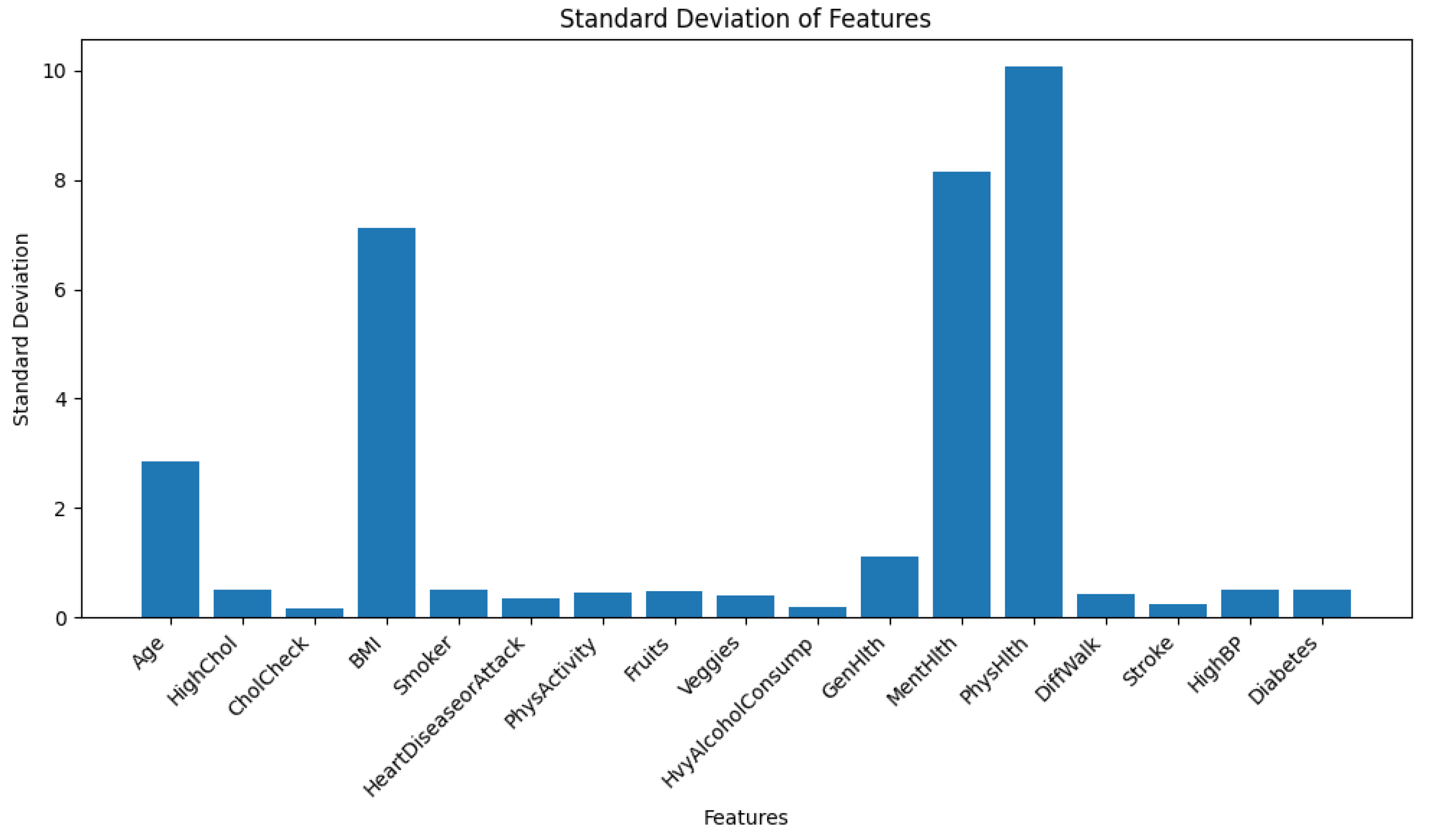
Figure 2.
Principal Component Analysis (PCA) Visualization Showing Class-Wise Distribution of Diabetes and Non-Diabetes Instances.
Figure 2.
Principal Component Analysis (PCA) Visualization Showing Class-Wise Distribution of Diabetes and Non-Diabetes Instances.
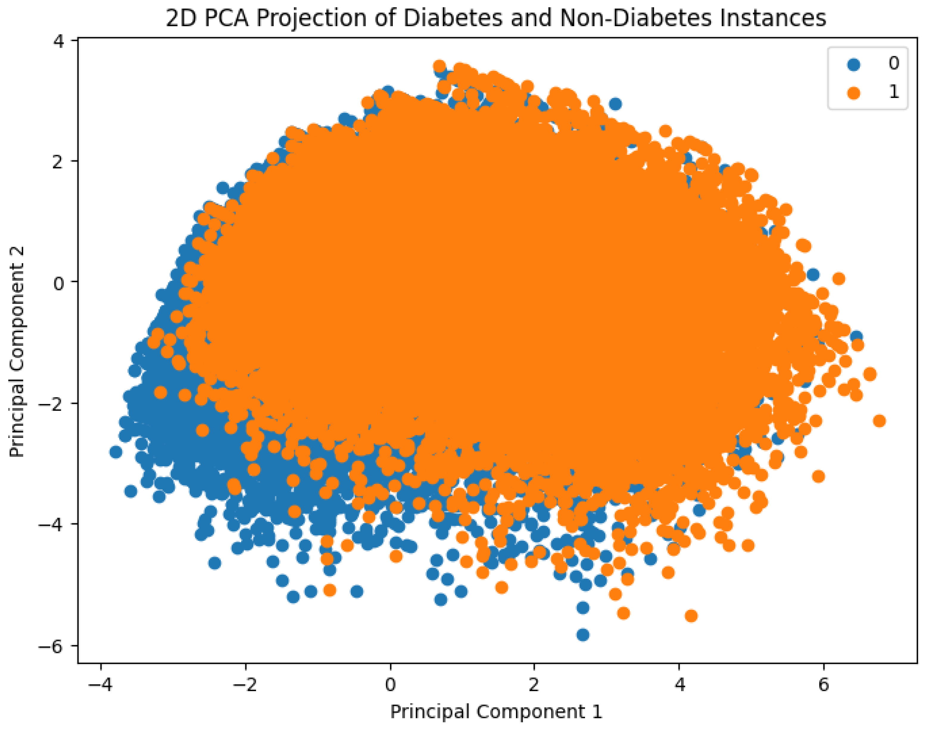
Figure 3.
Correlation Heatmap of the Features.
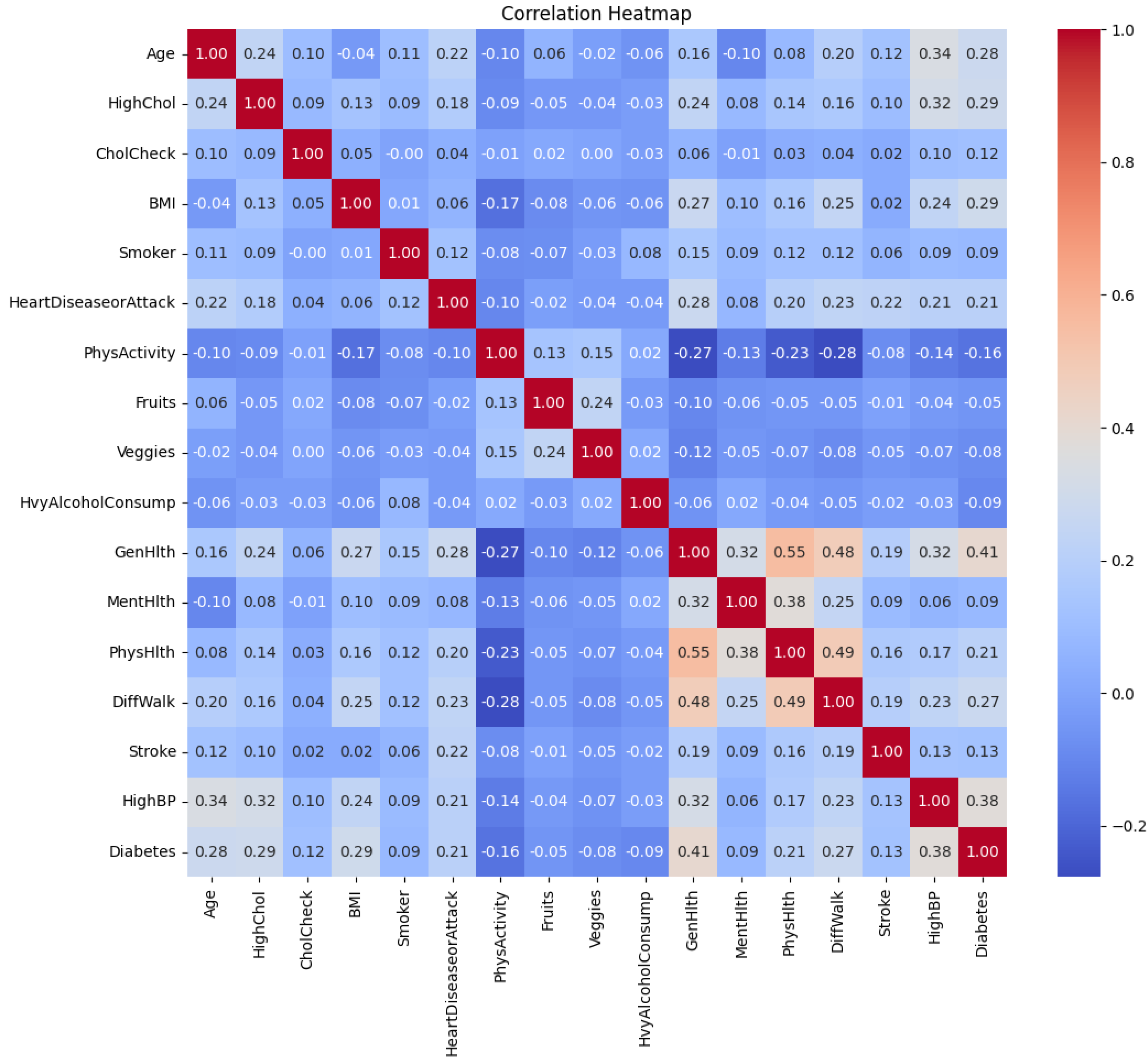
Figure 4.
Frequency of Diabetes (1) and Non-Diabetes (0) Instances in the Dataset
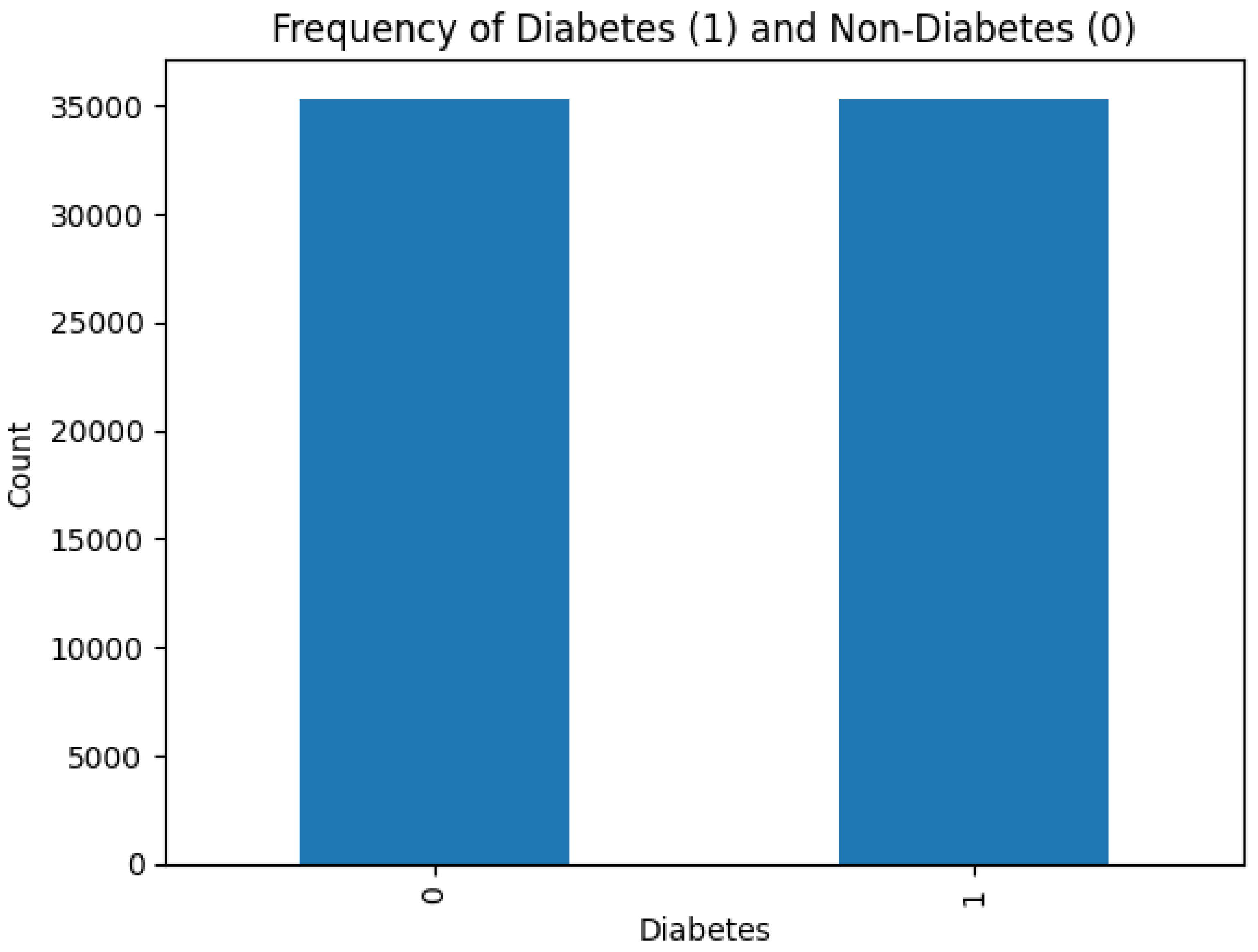
Figure 5.
ROC-AUC Curve of Three Ensemble Models

Figure 6.
ROC-AUC Curve of TabNet and CGSC
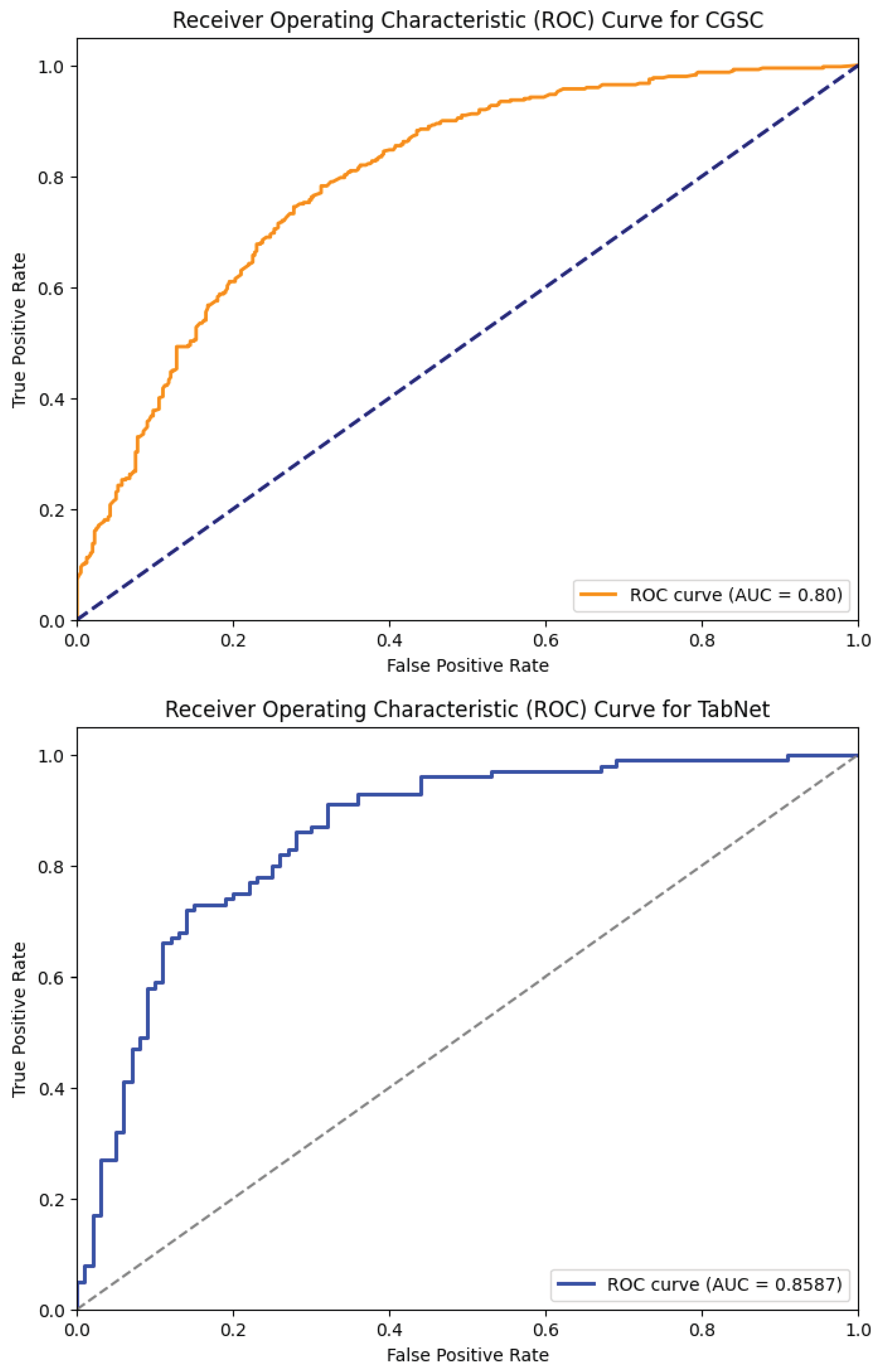
Figure 7.
F1-Score Uncertainty of the Ensemble Models
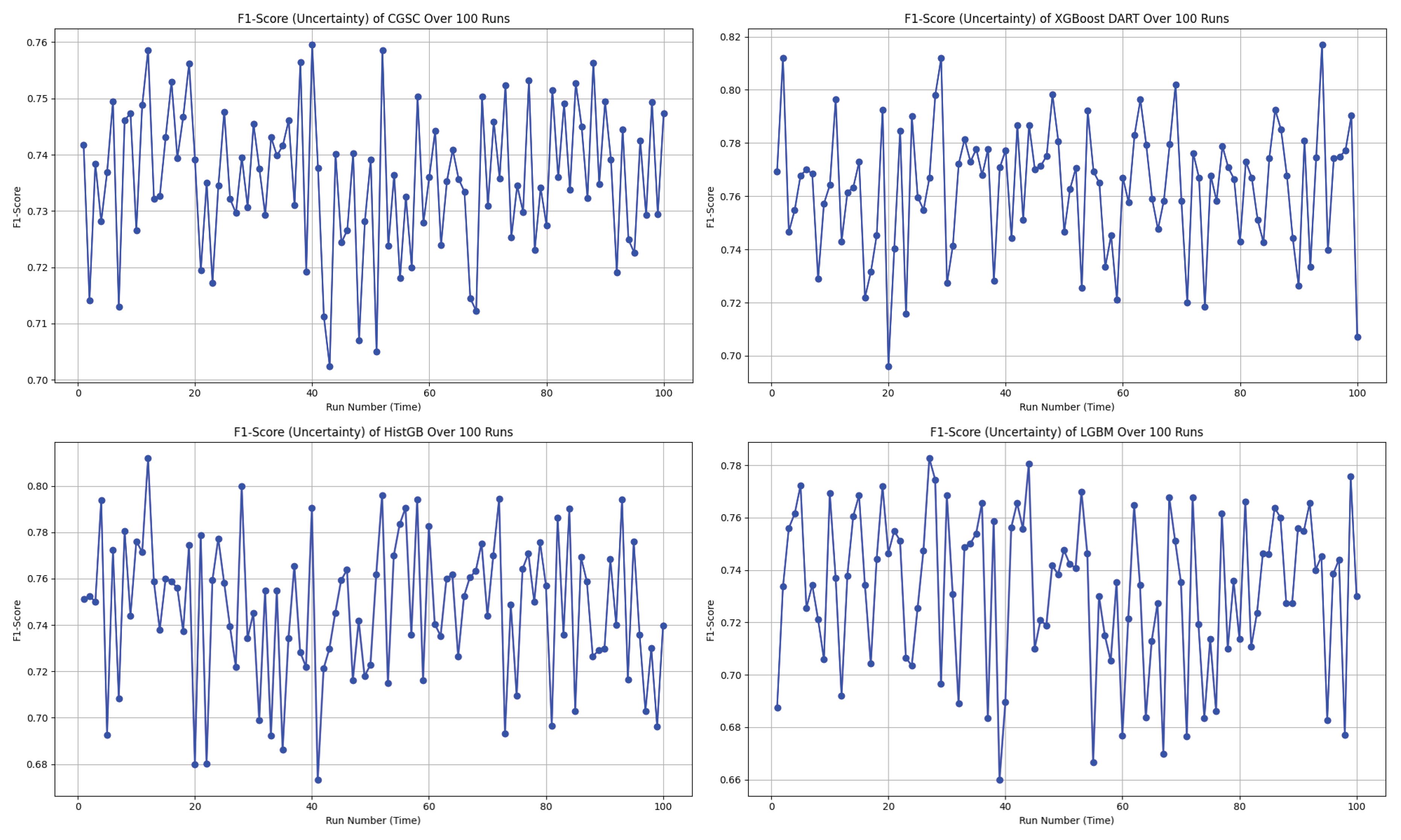
Figure 8.
SHAP summary plot showing global feature importance and influence direction in the XGBoost DART model for diabetes prediction. Red indicates higher feature values, blue indicates lower values.
Figure 8.
SHAP summary plot showing global feature importance and influence direction in the XGBoost DART model for diabetes prediction. Red indicates higher feature values, blue indicates lower values.
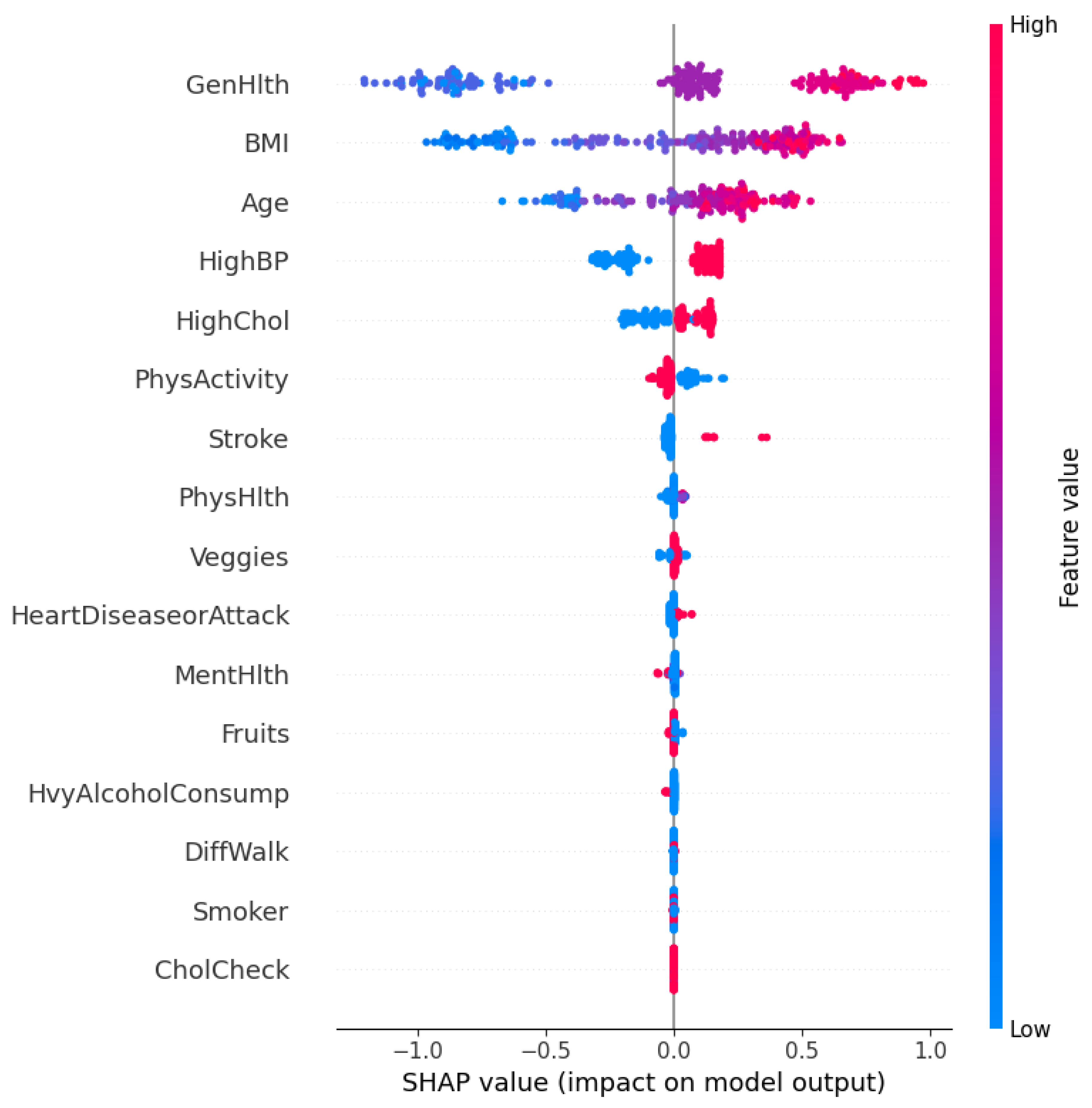
Figure 9.
Local SHAP explanation from XGBoost DART for an individual predicted as not diabetic (class 0). Each bar represents the feature’s contribution to pushing the model output away from the base value toward the final prediction .
Figure 9.
Local SHAP explanation from XGBoost DART for an individual predicted as not diabetic (class 0). Each bar represents the feature’s contribution to pushing the model output away from the base value toward the final prediction .
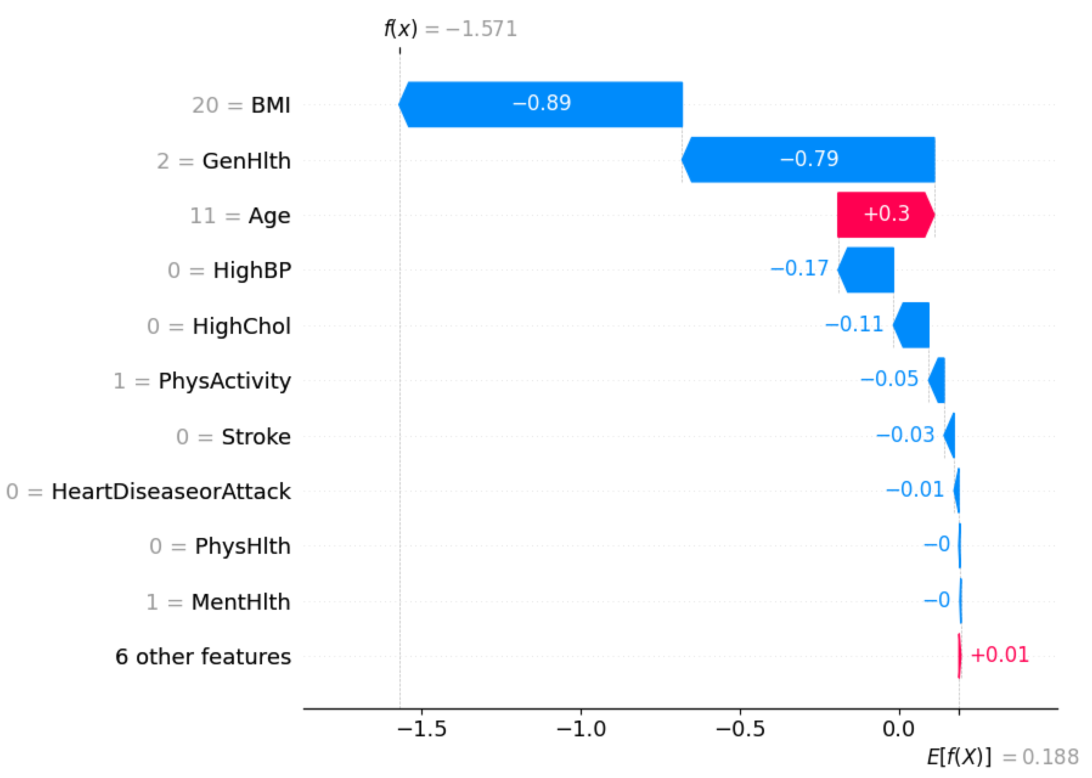
Figure 10.
Local SHAP explanation from XGBoost DART for an individual predicted as diabetic (class 1). Each feature’s SHAP value shows its influence in moving the prediction from the expected base value to the final output .
Figure 10.
Local SHAP explanation from XGBoost DART for an individual predicted as diabetic (class 1). Each feature’s SHAP value shows its influence in moving the prediction from the expected base value to the final output .
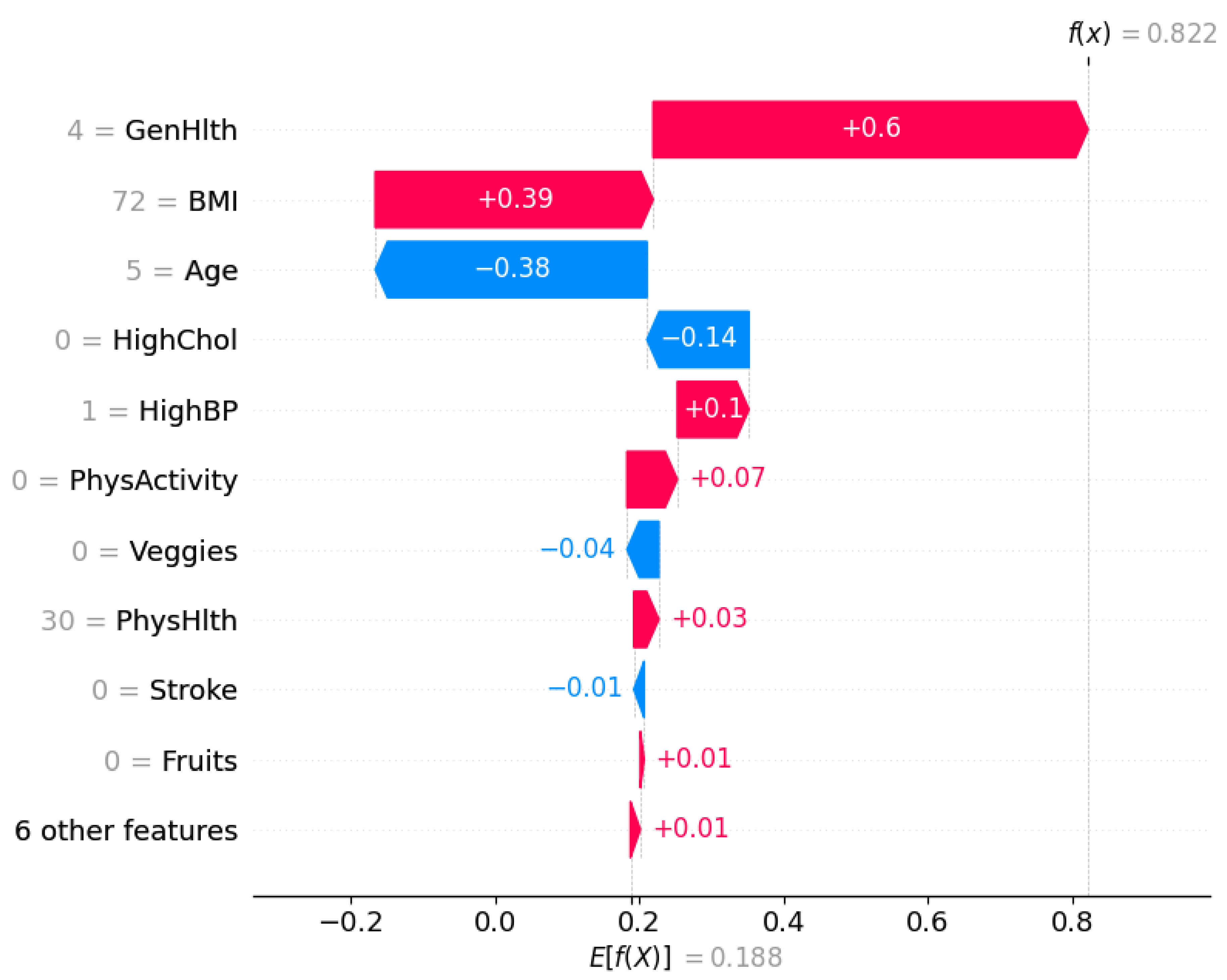
Figure 11.
Global Feature Importance by TabNet
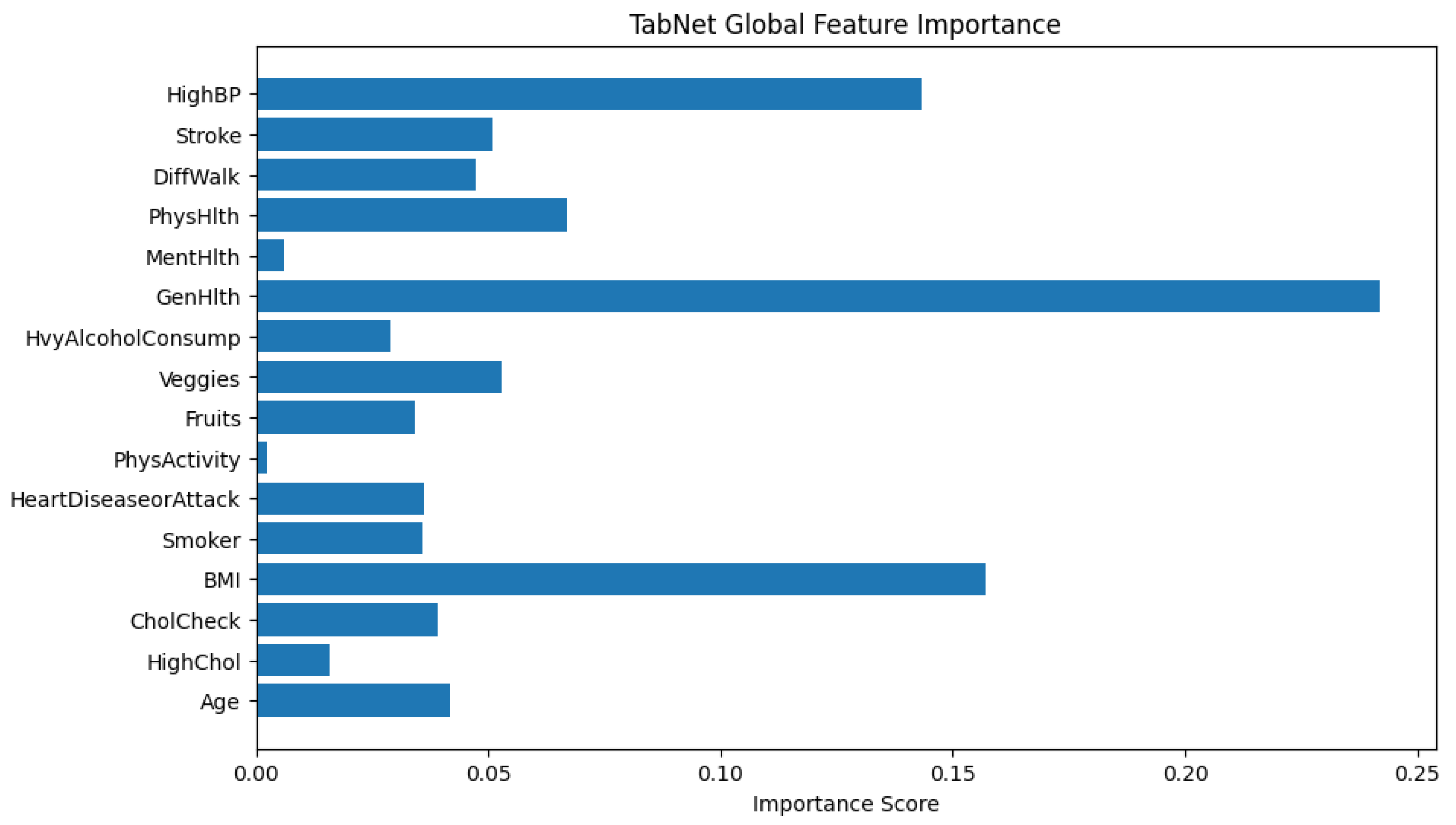
Figure 12.
TabNet Local Feature Importance Plot for an Individual Classified as Diabetic
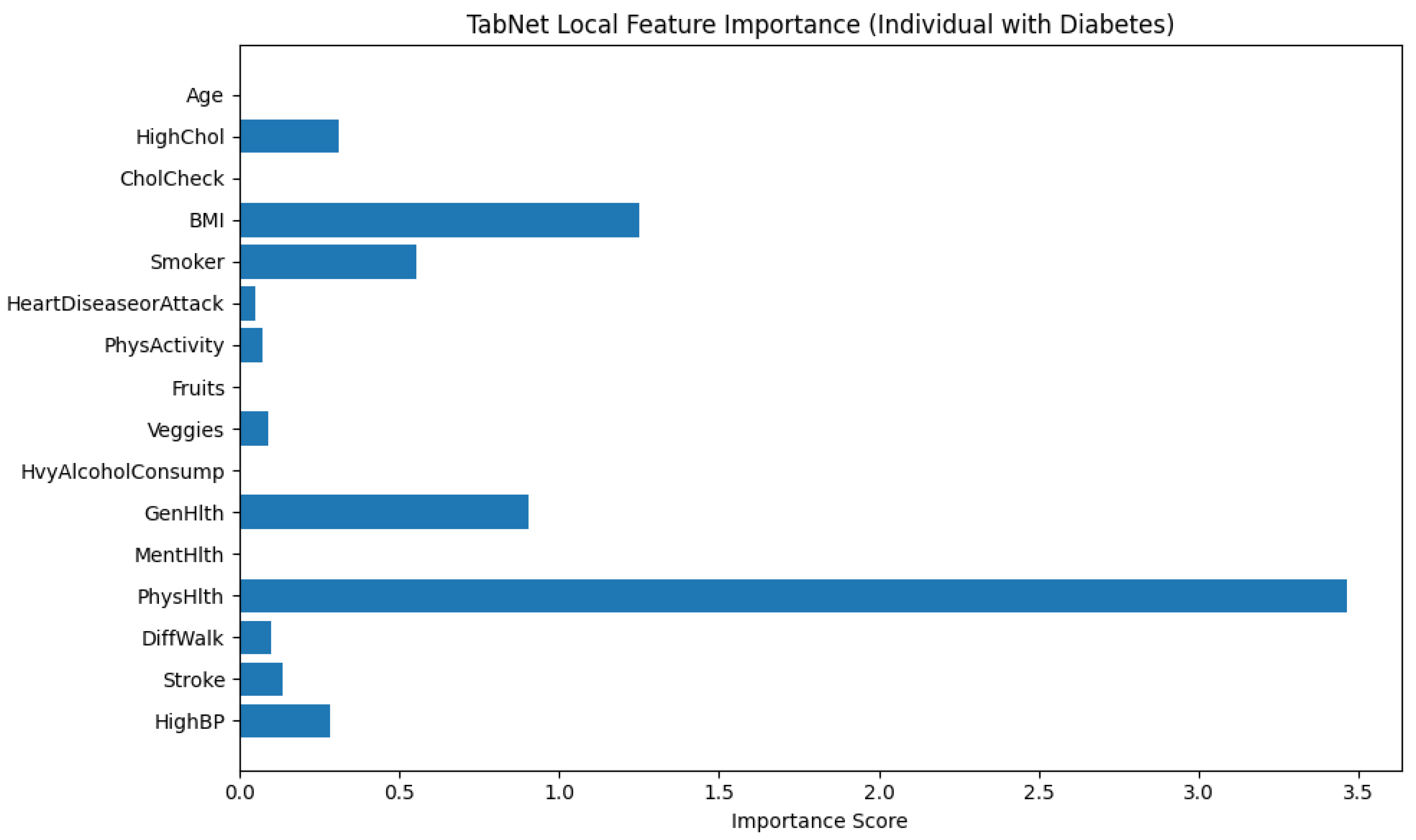
Figure 13.
TabNet Local Feature Importance for an Individual Predicted as Non-Diabetic
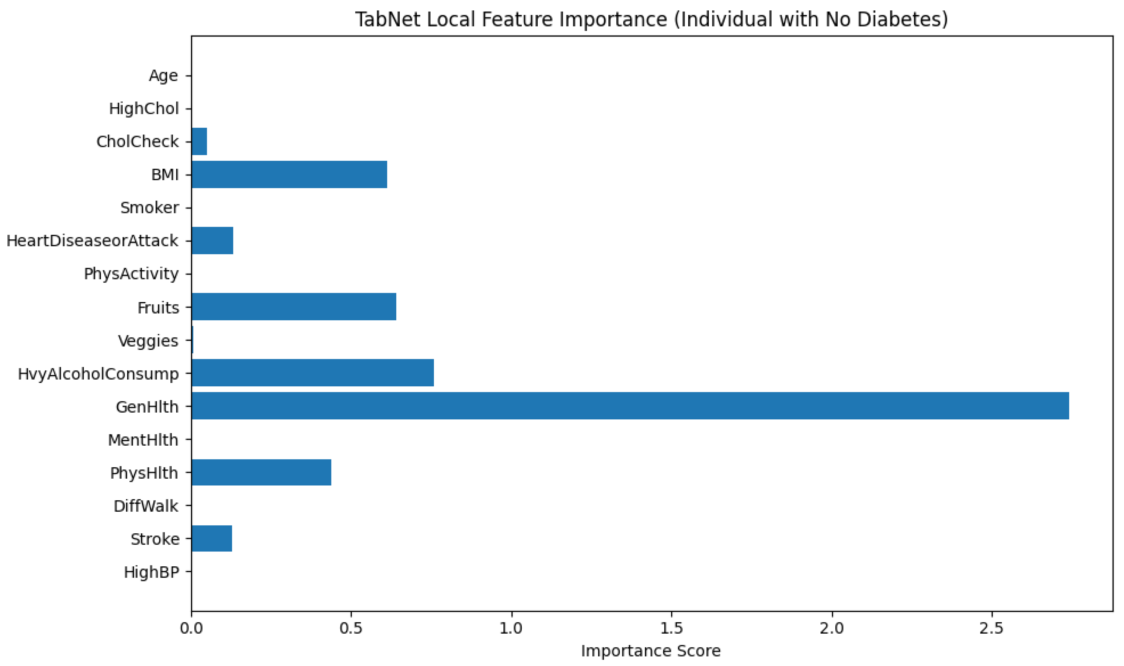
Figure 14.
Counterfactual examples generated by DiCE showing minimal changes needed to alter a prediction from non-diabetic (0) to diabetic (1)
Figure 14.
Counterfactual examples generated by DiCE showing minimal changes needed to alter a prediction from non-diabetic (0) to diabetic (1)
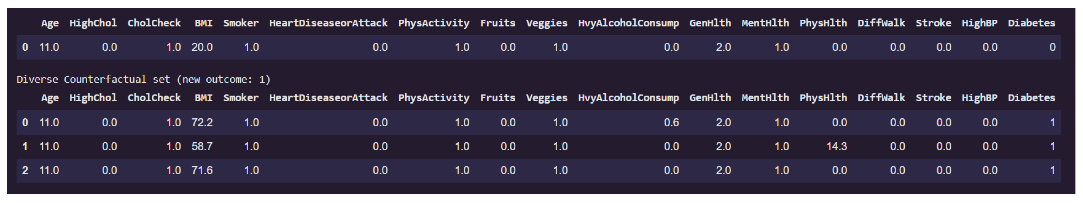
Figure 15.
Counterfactual examples generated by DiCE showing how an individual classified as diabetic (1) could instead be classified as non-diabetic (0) through a reduction in BMI.
Figure 15.
Counterfactual examples generated by DiCE showing how an individual classified as diabetic (1) could instead be classified as non-diabetic (0) through a reduction in BMI.
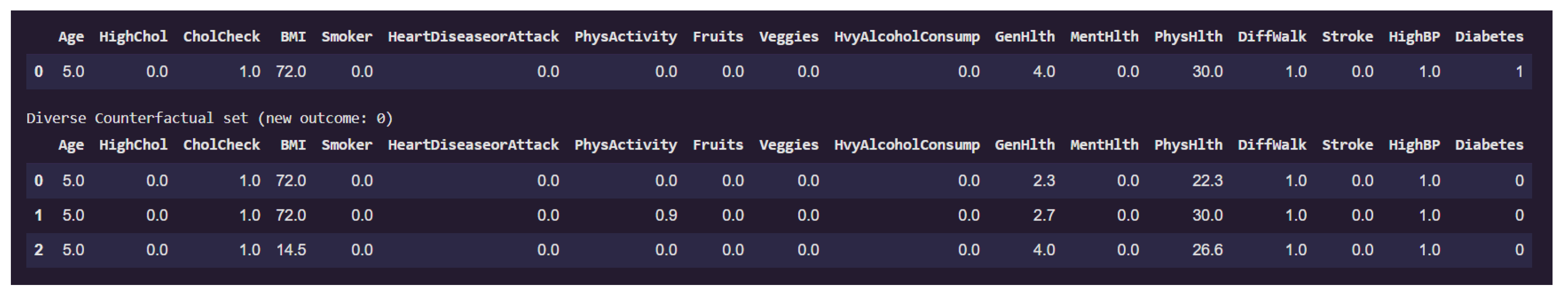
Figure 16.
Diverging Bar Chart of ATE by Feature
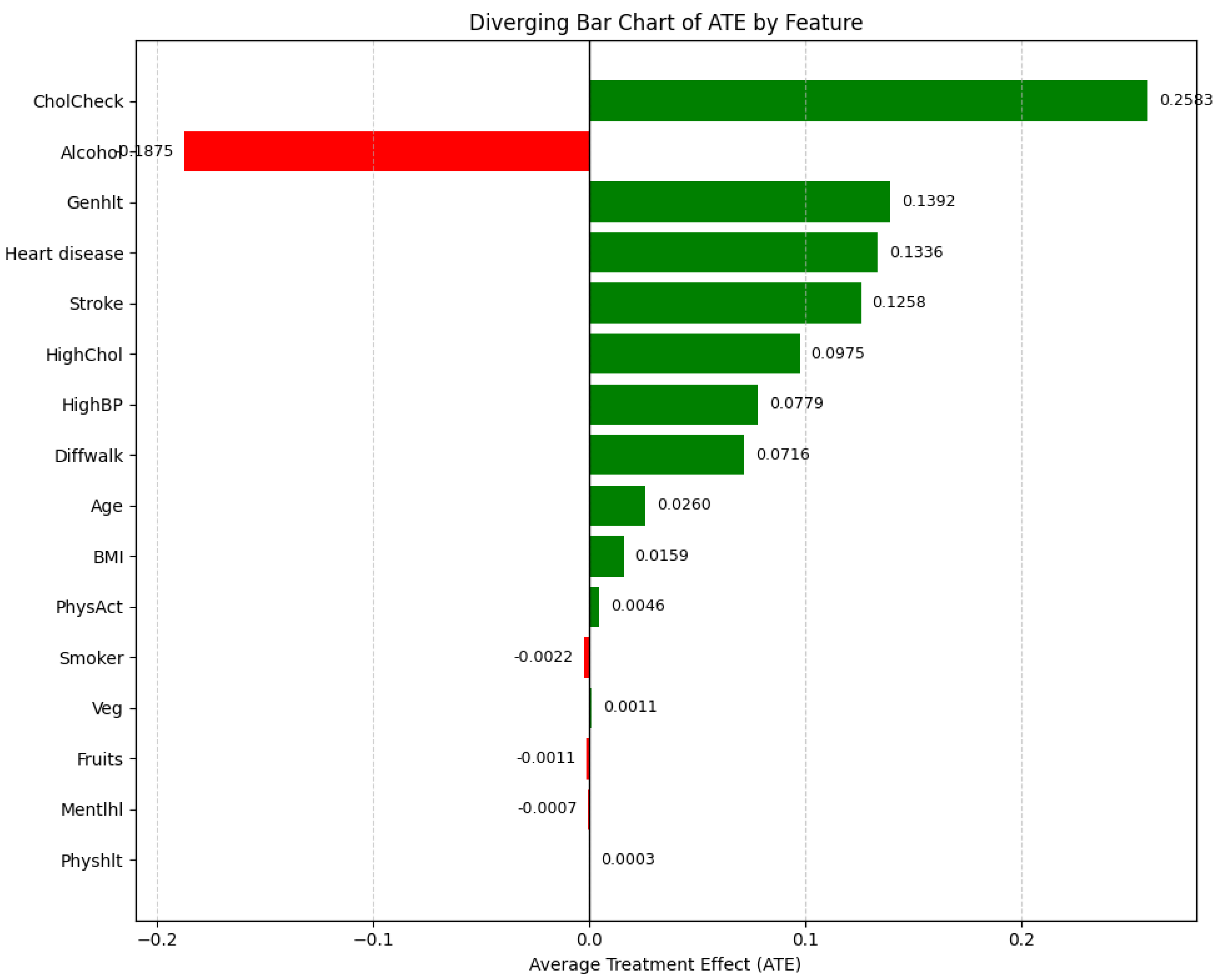

Table 1.
Variable Definitions and Encodings in the Diabetes Diagnosis Dataset
| Variable | Definition | Possible Values / Encoding |
|---|---|---|
| Age | Age group of respondent | Categorical (13 levels): 1 = 18–24; ...; 13 = 80+ |
| Sex | Biological sex of respondent | 0 = Female; 1 = Male |
| HighChol | Ever diagnosed with high cholesterol | 0 = No; 1 = Yes |
| CholCheck | Had cholesterol check in last 5 years | 0 = No; 1 = Yes |
| BMI | Body Mass Index | Continuous positive values |
| Smoker | Smoked at least 100 cigarettes in lifetime | 0 = No; 1 = Yes |
| HeartDisease | Ever diagnosed with heart disease or heart attack | 0 = No; 1 = Yes |
| PhysActivity | Physical activity outside of work | 0 = No; 1 = Yes |
| Fruits | Consumes fruit daily | 0 = No; 1 = Yes |
| Veggies | Consumes vegetables daily | 0 = No; 1 = Yes |
| Alcohol | Heavy alcohol consumption 1 | 0 = No; 1 = Yes |
| GenHlth | Self-rated general health | Ordinal: 1 = Excellent to 5 = Poor |
| MentHlth | Days of poor mental health (past month) | Integer: 0–30 |
| PhysHlth | Days of poor physical health (past month) | Integer: 0–30 |
| DiffWalk | Difficulty walking or climbing stairs | 0 = No; 1 = Yes |
| Stroke | Ever diagnosed with stroke | 0 = No; 1 = Yes |
| HighBP | Ever diagnosed with high blood pressure | 0 = No; 1 = Yes |
Defined as drinks/week for men and drinks/week for women.
Table 2.
Model Performance Comparison
| Model | Precision | Recall | F1-Score | Accuracy | AUC |
|---|---|---|---|---|---|
| XGBoost Dart | 0.76 | 0.80 | 0.78 | 0.78 | 0.84 |
| LightGBM | 0.71 | 0.76 | 0.73 | 0.72 | 0.97 |
| HistGB | 0.72 | 0.73 | 0.73 | 0.72 | 0.78 |
| TabNet | 0.79 | 0.73 | 0.76 | 0.77 | 0.86 |
| CGSC | 0.70 | 0.81 | 0.75 | 0.73 | 0.80 |
Disclaimer/Publisher’s Note: The statements, opinions and data contained in all publications are solely those of the individual author(s) and contributor(s) and not of MDPI and/or the editor(s). MDPI and/or the editor(s) disclaim responsibility for any injury to people or property resulting from any ideas, methods, instructions or products referred to in the content. |
© 2025 by the authors. Licensee MDPI, Basel, Switzerland. This article is an open access article distributed under the terms and conditions of the Creative Commons Attribution (CC BY) license (http://creativecommons.org/licenses/by/4.0/).
Copyright: This open access article is published under a Creative Commons CC BY 4.0 license, which permit the free download, distribution, and reuse, provided that the author and preprint are cited in any reuse.


