
Submitted:
04 May 2025
Posted:
06 May 2025
You are already at the latest version
Abstract
In this work, we present a training method for a Fully Quantum Neural Network (FQNN) based entirely on quantum circuits. The model processes data exclusively through quantum operations, without incorporating classical neural network layers. In the proposed architecture, the roles of classical neurons and weights are assumed respectively by qubits and parameterized quantum gates: input features are encoded into quantum states of qubits, while the network weights correspond to the rotation angles of quantum gates that govern the system’s state evolution. The optimization of gate parameters is performed using directional gradient estimation, where gradients are numerically approximated via finite differences, eliminating the need for analytic derivation. The training objective is defined as the quantum state fidelity, which measures the similarity between the network’s output state and a reference state representing the correct class.
Keywords:
Quantum Neural Networks
; Fidelity-based Training
; Fully Quantum Models
; Iris Dataset
1. Introduction
In recent years, we have witnessed a dynamic development of machine learning methods and neural networks, which have become the foundation of many breakthrough achievements in fields such as image recognition, natural language processing, and recommendation systems. However, the increasing size of datasets and the complexity of models have led to significant limitations of classical neural networks in terms of computational demands and scalability.
In response to these challenges, a new research domain has emerged—Quantum Machine Learning (QML)—which combines machine learning techniques with the potential of quantum computing [1,2,3]. Quantum computers, thanks to properties such as superposition and entanglement, offer information processing capabilities that may outperform classical systems in selected tasks [4].
One of the most promising directions in QML is the development of Quantum Neural Networks (QNNs) [5]. These models employ quantum circuits for data processing, where qubits take the role of classical neurons, and parameterized quantum gates serve as analogues of weights. In most existing approaches, QNN architectures are hybrid in nature—some parts of the data processing or optimization are performed classically, which limits the full exploitation of quantum computational potential [6,7].
In this study, we propose an alternative approach: a Fully Quantum Neural Network. Our model is based entirely on quantum operations, without the use of classical neural layers. In the proposed architecture, input features are encoded into qubit states, while network weights correspond to the rotation angles of quantum gates. The network structure consists of several quantum layers, each involving rotations based on input features and weights, as well as entangling operations implemented via controlled-rotation (CRY) gates. Analogous to classical neural networks, quantum layers transform the input state into progressively more complex representations in feature space, enabling effective classification.
The FQNN training process is carried out through directional gradient-based optimization of quantum gate parameters, using quantum state fidelity as the objective function. The gradients are estimated numerically via finite difference methods, eliminating the need for analytic derivative computation. The experiments were conducted using the Qiskit AerSimulator quantum simulator, which enables accurate emulation of quantum circuit behavior in a classical environment.
The aim of this study is to design and evaluate an FQNN for the task of classifying data from the classical Iris dataset. We assess the learning effectiveness of the network, the stability of the optimization process, and the achieved classification accuracy, thereby demonstrating the practical applicability of fully quantum architectures in machine learning tasks without reliance on classical processing layers.
2. Architecture Description FQNN
The Fully Quantum Neural Network (FQNN) proposed in this work has been designed as a sequence of quantum layers in which input information is encoded and processed exclusively through quantum circuits. The network consists of the following components:
- Data encoding: Each input feature is encoded into a single qubit using a rotation operation , where the rotation angle is proportional to the feature value. This process enables the embedding of classical data into the quantum state space.
- Quantum weight layer: The network’s weights are represented by additional qubits, each subjected to an independent quantum rotation , with the rotation angles corresponding to trainable network parameters. These angles play a role analogous to classical weights in conventional neural networks.
- Entanglement: For each data–weight qubit pair, controlled gates are applied to introduce entanglement between the data and weight states. This mechanism allows the network to capture nonlinear dependencies among input features.
- Label encoding and error measurement: To perform classification, the network prepares a quantum state corresponding to the target label. The similarity between the output state of the network and the reference label state is evaluated using the swap-test procedure.
2.1. Data Encoding
The goal of data encoding in a quantum neural network is to map classical input feature values (scaled to the range[0,1]) onto appropriate quantum states of qubits, thereby enabling further quantum processing.
Feature-to-Qubit Rotation Assignment
In the FQNN, each input feature is assigned to a single qubit and encoded via a rotation around the Y-axis of the Bloch sphere using the gate. The rotation gate around the Y-axis is defined by the following matrix operator:
where:
- is the rotation angle,
- Y is the Pauli-Y matrix:
Qubit State Transformation
A qubit is initialized in the ground state :
After applying the gate, the qubit state becomes:
Given that in the network:
each feature is linearly scaled to a rotation angle within the interval .
After substituting the angle , the qubit state takes the following form:
This implies that:
- If , the qubit remains in the state .
- If , the qubit is rotated to the state .
- For intermediate values of , the qubit is in a superposition of and .
Vector Representation of the Entire Input Encoding
Assuming there are N features , after encoding all features, the full initial data state is given by the tensor (Kronecker) product of all individually encoded qubits:
Through this encoding:
- The classical feature values control the amplitudes of the quantum states.
- The input data are transformed into a superposition of quantum states, which can then be further modified through quantum operations (rotations, entanglement).
This encoding does not alter the classical information itself but extends it into a Hilbert space of dimension , enabling the modeling of more complex relationships among features than classical networks can achieve.
2.2. Quantum Weight Layer in FQNN
The purpose of the quantum weight layer is to introduce trainable parameters into the network, analogous to the weights in classical neural networks. In classical networks, weights define the strength of connections between neurons, influencing the outcome of signal propagation. In an FQNN, this role is assumed by the rotation angles of quantum gates acting on separate weight qubits.
Layer Structure
In the quantum weight layer, each weight qubit:
- is initialized in the state ,
- undergoes a rotation around the Y-axis using a quantum gate,
- where the parameter is an independent network parameter optimized during training.
Mathematically:
where:
- is the parameter (weight) assigned to the j-th weight qubit,
- Y is the Pauli-Y matrix.
Applying to a qubit initialized in the state yields:
Weight Parameterization
Each weight parameter is independently optimized based on the results of the swap-test and the learning process.
- Initially, the parameters are randomly initialized within the interval .
- During training, the values of are updated in the direction that increases the fidelity between the network’s output state and the target label state.
2.3. Interpretation of the Role of Weights in FQNN
In a classical neural network:
- Weights control how strongly input features influence subsequent layers and the final prediction outcome.
In the proposed FQNN:
- The weights (rotation angles ) determine the extent to which the state of a weight qubit is "tilted" from towards .
- Subsequently, during the entangling operation (CRY gate), the state of the weight qubit governs the influence on the data qubits, modifying their amplitudes accordingly.
2.4. Vector Representation of the Weight Layer
Assuming M weight qubits with parameters , the state of the entire quantum weight layer can be expressed as:
which corresponds to the tensor product of the individual weight qubit states.
3. Entanglement in FQNN
Entanglement in a quantum neural network serves to establish nonlinear dependencies between input features and quantum weights.
- In classical neural networks, nonlinearity is introduced via activation functions (e.g., ReLU, sigmoid).
- In FQNNs, nonlinearity and correlations are achieved through entangling operations between data qubits and weight qubits.
3.1. How Entanglement is Implemented in FQNN
In the proposed model, entanglement is implemented using controlled rotation gates :
- The weight qubit acts as the control qubit,
- The data qubit acts as the target qubit,
- The operation applies a rotation to the data qubit only if the weight qubit (control) is in the state.
Symbolically, if is the control qubit and is the target qubit, the operation is defined as:
where:
- I is the identity matrix (no change if the control qubit is in the state),
- is a rotation by angle on the target (data qubit) when the control qubit is in the state.
3.2. Mathematical Action of
For a pair of two qubits, the initial state can be written generally as:
After applying the gate, the transformation proceeds as follows:
- If the control qubit is in the state: no change occurs.
- If the control qubit is in the state: a rotation is applied to the target qubit.
Specifically:
3.3. Intuitive Meaning of Entanglement
Data qubits and weight qubits become entangled — their quantum states become interdependent.
- Data qubits do not merely encode their input feature values; their quantum evolution is influenced by the states of the weight qubits (i.e., the learned parameters).
- This entanglement introduces nonlinear correlations between the input features and model parameters, serving a role analogous to activation functions and signal propagation mechanisms in classical neural networks.
4. Label Encoding and Error Measurement in FQNN
In classical machine learning, a label indicates the class membership of a given sample. In the proposed FQNN, the label is not stored as a discrete value (e.g., "0", "1", or "2"), but is instead represented as a quantum state encoded across two qubits.
Label Encoding:
The label encoding procedure involves preparing a quantum register in a specific quantum state corresponding to the target class. This encoded label state is later compared to the output state of the network using the swap-test.
This approach enables error evaluation in terms of quantum state similarity rather than direct numerical comparison, which aligns with the principles of quantum information processing.
4.1. Label Encoding Scheme
Each class label y is encoded using two qubits as follows:
- The state corresponds to class 0,
- The state corresponds to class 1,
- The state corresponds to class 2.
Formally, for each class y, the label state is prepared as:
The preparation of the appropriate label state is carried out using X (NOT) gates on the corresponding qubits:
- If a component of the desired label state is "1", an X gate is applied to the corresponding qubit.
Example: For label 2:
- The first qubit (qubit 0) is set to using an X gate,
- The second qubit (qubit 1) remains in the state (no operation needed).
4.2. State Comparison – Error Measurement
The swap-test is a quantum algorithm used to determine the similarity between two quantum states and . The goal of the procedure is to estimate the fidelity, defined as [8]:
The algorithm requires one ancillary qubit prepared in a superposition state using a Hadamard gate, along with two quantum registers representing the states and .
The swap-test procedure is as follows:
- Prepare the ancillary qubit in a superposition state:
- Apply controlled-swap (CSWAP) operations between corresponding qubits of and , controlled by the ancillary qubit.
- Apply a second Hadamard gate to the ancillary qubit.
- Measure the ancillary qubit.
The probability of measuring the ancillary qubit in the state is:
Thus, the fidelity can be extracted as:
In the presented FQNN model, the swap-test is used to evaluate the similarity between the network’s output state and the target label state. A high fidelity value indicates a successful classification, and swap-test measurements directly guide the optimization process of the network parameters.
After encoding the label, a swap-test is performed between:
- the output state of the network ,
- and the label state .
The swap-test measures the fidelity:
which quantifies the similarity between the network’s prediction and the correct label.
4.3. Error Measurement Algorithm and Its Role in Training
If the swap-test yields a high fidelity (), it indicates that the network has correctly classified the input sample. If the fidelity is low, it means that the network has made a classification error.
During training, the average fidelity across the dataset is used as an indicator of prediction quality.
Objective Function:
In the proposed FQNN, the objective function is not based on a classical loss function (such as cross-entropy). Instead, training is driven by maximizing the average fidelity between the network’s output states and the corresponding label states.
Thus, error measurement in FQNN involves:
- minimizing the difference between the network output state and the target label state,
- maximizing the swap-test result (i.e., the fidelity).
8. Training and Optimization
The training process of the Fully Quantum Neural Network is based on optimizing the rotation parameters of quantum gates, which represent the network’s weights. Due to the quantum nature of computation and the lack of direct access to derivatives of the objective function, this work adopts a finite-difference directional gradient approach for gradient estimation [9].
5. Training Procedure Overview
Each training epoch consists of the following steps:
Gradient Estimation:
For each weight , two small variations are considered: a positive shift and a negative shift , where is a dynamically adjusted update step. For both perturbations, the average fidelity (i.e., average swap-test result) is computed over a small mini-batch of training samples.
Direction Selection:
The update direction is determined by comparing the fidelities:
- If , the weight is updated in the positive direction.
- If , the update direction is negative.
Weight Update:
Weights are updated based on the chosen direction:
where indicates the direction of the update for the j-th weight.
Step Size Adaptation:
Every few epochs (e.g., every 5 epochs), the values of are reduced by multiplying them with a decay factor (e.g., 0.9), allowing for finer tuning of the parameters as the model approaches convergence.
5.1. Objective Function and Quality Metric
The objective function for the training process is to maximize the average fidelity between the network output state and the encoded label state :
The average fidelity over a mini-batch is used as an estimator of prediction quality when evaluating different parameter updates.
Additionally, the classification accuracy on the test set is measured after each epoch to verify the effectiveness of the learning process.
5.2. Optimization Strategies
Mini-batch learning:
To accelerate the training process and increase the stability of gradient estimation, swap-tests are performed on randomly selected small subsets (mini-batches) of the training data (e.g., 5 samples per batch).
Adaptive step-size reduction (delta annealing):
The dynamic reduction of the update step size enables more precise fine-tuning of the weights in the later stages of training, minimizing the risk of oscillations around the optimum.
Batch randomization:
At the beginning of each epoch, the training examples are randomly shuffled, which helps reduce the risk of overfitting to a specific data distribution.
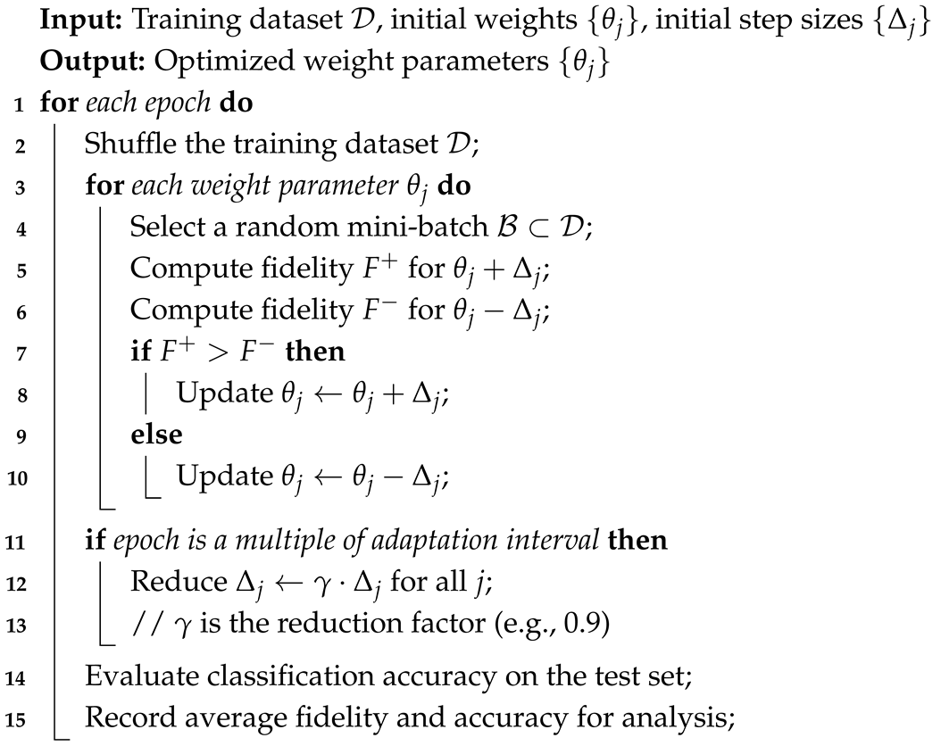
5.3. Pseudocode of the Training Procedure
To provide a clear and structured overview of the training methodology applied in the Fully Quantum Neural Network, this section presents the pseudocode for the optimization algorithm. The pseudocode outlines the main steps of the learning process, including gradient estimation via finite differences, weight updates based on fidelity maximization, and adaptive adjustment of the update step size.
This high-level representation facilitates a better understanding of the iterative learning dynamics before proceeding to the detailed description of experimental implementation and evaluation.
| Algorithm 1: Training Procedure for Fully Quantum Neural Network (FQNN) |
 |
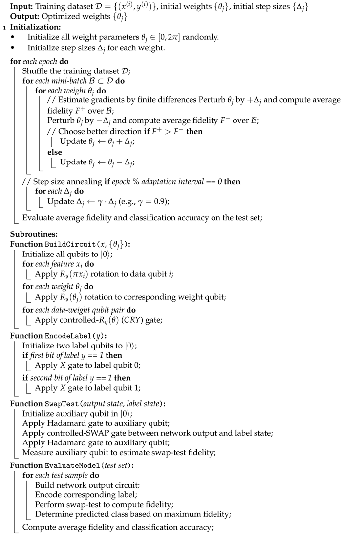
6. Pseudocode of Fully Quantum Neural Network (FQNN)
This section presents the pseudocode of the Fully Quantum Neural Network training and inference procedure. The pseudocode summarizes the main steps of the method, including quantum data encoding, weight initialization, network construction, fidelity-based optimization, and model evaluation. It serves as a concise, high-level description of the complete quantum learning process implemented in this work.
| Algorithm 2: Full Training and Evaluation Procedure for Fully Quantum Neural Network (FQNN) |
 |
7. Experimental Setup
7.1. Input Data
The experiments were conducted on the Iris dataset, consisting of 150 examples described by four numerical features: sepal length, sepal width, petal length, and petal width. Each example belongs to one of three classes representing different species of Iris flowers.
Prior to training, the data were scaled individually for each feature to the range using Min-Max Scaling.
The dataset was then split into a training set (80%) and a test set (20%), maintaining proportional class distribution through stratified sampling.
Simulation Environment
All experiments were conducted using the Qiskit AerSimulator quantum simulator. Simulations were performed in a noise-free environment, with the default implementation of ideal quantum gates. Each quantum circuit was executed 3000 times (shots = 3000) to obtain stable statistical results during swap-test measurements.
7.2. FQNN Architecture
The designed FQNN architecture consisted of:
- 4 qubits representing the input data features,
- 4 qubits representing the quantum weights,
-
3 auxiliary qubits:
- –
- 2 qubits for encoding the class label,
- –
- 1 qubit for performing the swap-test.
In total, the quantum circuit involved 11 qubits. The number of network layers was determined based on the ratio of the number of parameters to the number of input features, resulting in a three-layer quantum network.
7.3. Training Parameters
The training parameters were configured as follows:
- Number of training epochs: 12,
- Initial weight update step:
- Every 5 epochs, the values of were reduced by a factor of 0.9 (delta annealing),
- In directional gradient estimation, mini-batches of 5 randomly selected training samples were used for each parameter update.
7.4. Performance Evaluation Metrics
The model’s performance was evaluated using two main metrics:
- Average fidelity: the fidelity value from the swap-test between the FQNN output state and the encoded label state, calculated on selected training samples,
- Classification accuracy: the percentage of correctly classified examples on the test set, measured after each epoch.
Repeated Trials
To ensure the statistical reliability of the results and mitigate variance due to parameter initialization, the FQNN training process was repeated 20 times.
Each run was initialized independently and trained for 12 epochs using the same configuration and data splits. All reported performance metrics (fidelity, accuracy, delta values) were averaged over these 20 runs.
Where applicable, standard deviation bands or min–max ranges were included in plots to illustrate the consistency and stability of the training process across runs.
8. Results and Discussion
8.1. Best Performing Run
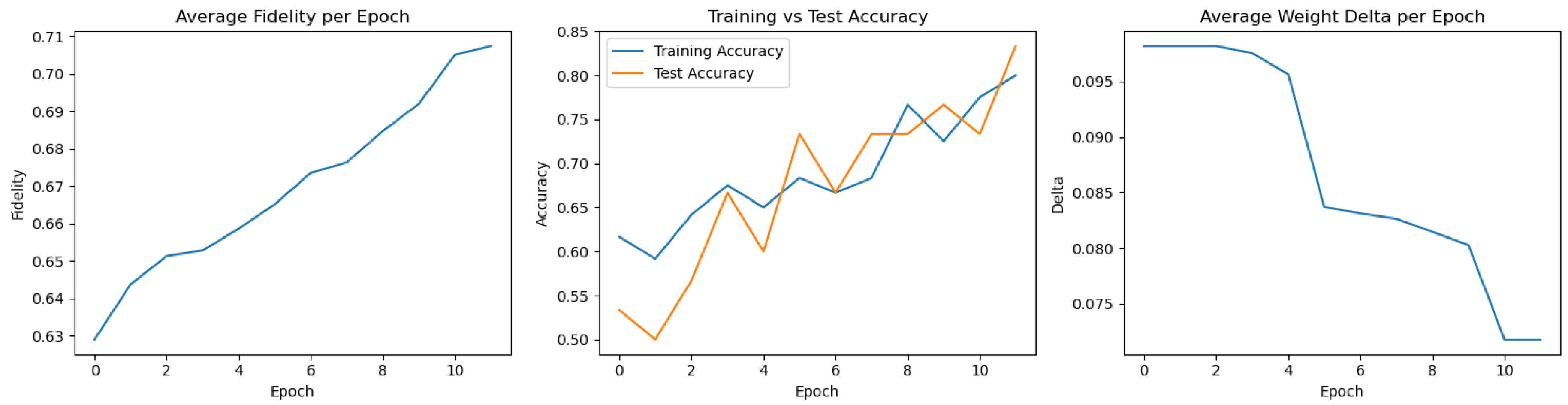
Among the 20 independent executions, multiple runs achieved the highest test accuracy of 96.67%. However, Run 12 was selected as the representative best-performing case, as it also exhibited the highest training accuracy (89.17%) and stable convergence behavior throughout all epochs.
Figure 1 demonstrates a clear and steady increase in fidelity and accuracy, confirming the effectiveness of the directional gradient method combined with delta annealing. The network shows both high expressiveness and generalization capability, making this configuration a strong candidate for practical applications.
Table 1 lists the final classification results for the best-performing FQNN run (Run 12), which achieved a test accuracy of 96.67%. Out of 30 test samples, 29 were correctly classified, with only one misclassification (sample 11: predicted class 0 instead of 2). This confirms that the network learned a highly effective decision boundary between the three Iris classes.
The test set includes a balanced mixture of examples from all three classes. The high accuracy and precision of prediction indicate that the FQNN is capable of generalizing well beyond the training data, even with a limited number of epochs and parameters.
8.2. Worst Performing Run
Despite identical training conditions, this run showed slower fidelity growth and lower test accuracy. The variability may stem from suboptimal initial parameters or mini-batch selection. Notably, delta values still decreased, suggesting proper optimization dynamics.
Table 2 presents the final classification results of the worst-performing run (Run 18), which achieved a test accuracy of 83.33%. Despite correct classification of most samples, the model failed on several instances belonging to class 2, misclassifying them as class 0.
This run highlights the sensitivity of the FQNN training process to initial quantum parameter configurations and optimization dynamics. The fidelity values in this run grew more slowly compared to others, and the network struggled to form clear class boundaries for complex decision surfaces. Nevertheless, the model preserved basic discrimination ability and converged toward reasonable accuracy after 12 epochs.
Figure 2.
Metrics from the worst performing FQNN training run (Run 18).
8.3. Aggregated Results Across 20 Training Runs
Figure 3 illustrates the evolution of average fidelity across training epochs for 20 independent FQNN training runs. Each line represents a separate execution with different random initialization of quantum gate parameters.
All runs show a clear upward trend in fidelity, indicating successful learning of the target label states. The gradual increase confirms that the quantum circuit is progressively aligning its output state closer to the encoded class state. Most runs converge to fidelities above 0.75, with some reaching 0.80 or higher by the final epoch.
Although minor variance in the convergence rate is visible (e.g., Run 8 exhibits slower improvement), the overall consistency across runs suggests that the training method is robust and repeatable. This validates the effectiveness of fidelity-based optimization using directional gradient estimation.
Figure 4 presents the test set classification accuracy obtained during 20 independent executions of the FQNN training process. Despite variations in initialization and stochastic mini-batch selection, most runs exhibit consistent improvement in accuracy over epochs.
The convergence behavior demonstrates the general robustness of the model, with the majority of runs exceeding 85% test accuracy by the final epoch. A few outliers with slower convergence (e.g., Run 8 or Run 17) reflect sensitivity to initial conditions or local optima, but the overall trend indicates high reliability and reproducibility.
This multi-run visualization provides strong evidence that the FQNN can learn effective class boundaries across different training conditions, reinforcing the utility of the quantum fidelity-based learning paradigm.
Table 3 summarizes the final training and test set classification accuracies for 20 independent runs of the FQNN model. Each run consisted of 12 training epochs using identical hyperparameters and architecture, but with randomly initialized quantum weights.
The training accuracy values exhibit low variance, with a mean of 0.8642 and a standard deviation of approximately 0.0201, indicating consistent convergence across runs. The test accuracy remains high overall, with a mean of 0.9350 and standard deviation of 0.0324.
Most runs achieve test accuracy above 0.93, confirming that the FQNN model generalizes well to unseen data. One notable outlier (Run 18) yielded a lower test accuracy (0.8333), which may be attributed to unfavorable initialization or mini-batch sampling.
Overall, the results demonstrate that the quantum model not only trains stably but also generalizes effectively across repeated trials, validating the fidelity-based training strategy.
Detailed plots for each of the 20 training runs, including fidelity, accuracy, and delta progression, are provided in Appendix A. These visualizations further confirm the stability and variability of the FQNN training process across different random initializations.
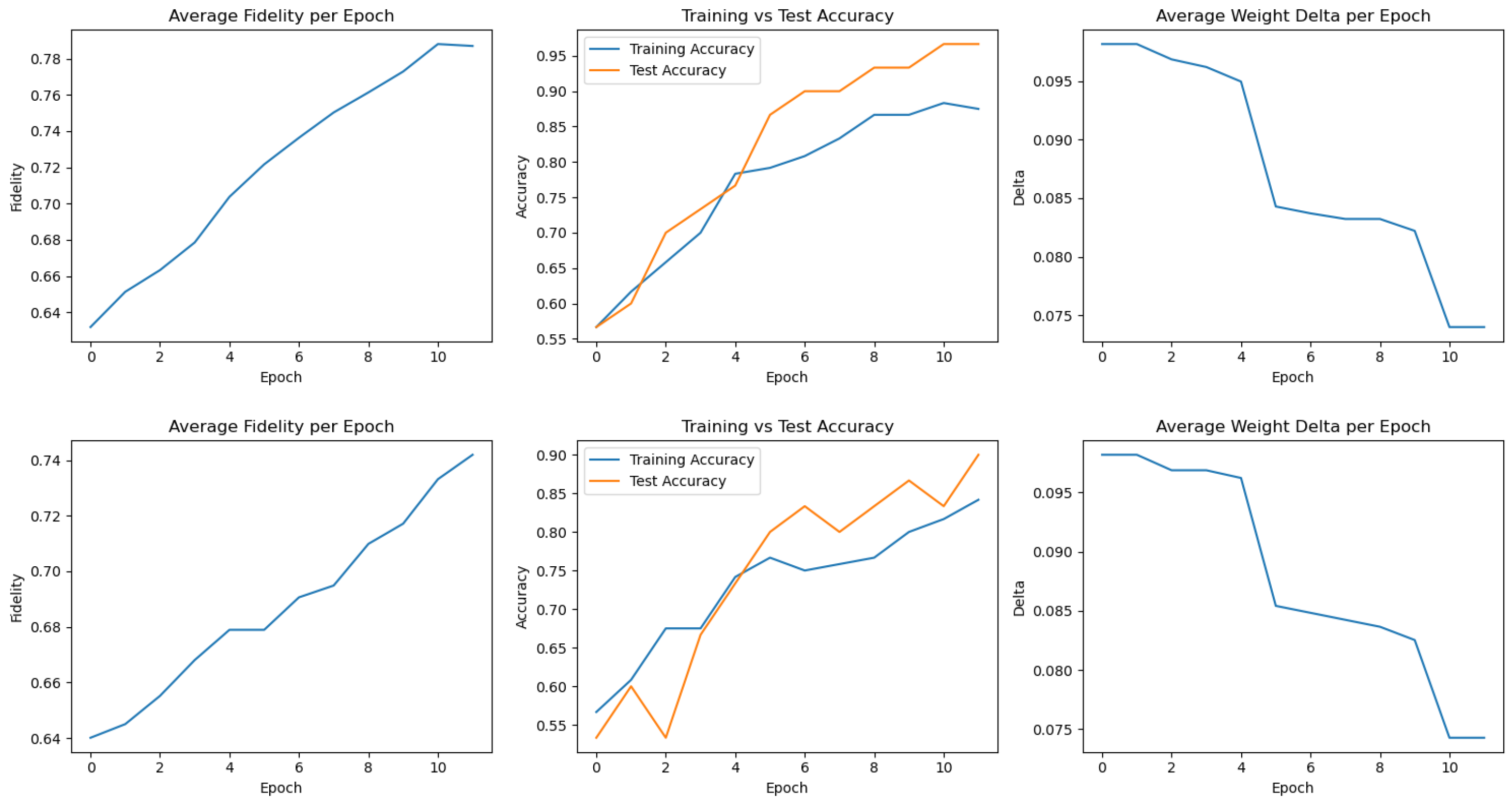
Training metrics for Runs 1–6 are shown in Figure A1, Runs 7–12 in Figure A2, Runs 13–18 in Figure A3, and the final set, Runs 19–20, in Figure A4.
Together, these plots illustrate the general trend of increasing fidelity and accuracy over epochs, as well as the consistent decay of parameter update deltas. They also reveal individual variations between runs, such as slower convergence or temporary drops in fidelity, which underline the stochastic nature of training but do not hinder overall model effectiveness.
8.4. Summary and Insights
The Fully Quantum Neural Network model demonstrated reliable and stable training behavior across 20 independent runs. Despite stochastic initialization and sampling, the training process consistently converged toward high classification accuracy and fidelity values.
In the best-performing run, the network achieved a test accuracy of 96.67% and training accuracy above 89%, while maintaining smooth fidelity growth across all epochs. Even in the worst case, the model retained a test accuracy of 83.33%, indicating that the network was still able to capture meaningful class boundaries.
The quantum-native training approach based on fidelity maximization and directional gradient updates proved to be both efficient and robust. The use of swap-test-based fidelity as an objective function directly aligns quantum state similarity with classification success, offering a natural and interpretable learning criterion for quantum models.
The proposed FQNN achieved competitive performance on the Iris dataset using only quantum operations, without reliance on classical neural layers. This supports the viability of fully quantum machine learning pipelines and motivates further exploration of scalable quantum architectures.
9. Conclusions
This study demonstrates the feasibility and effectiveness of training a Fully Quantum Neural Network for multi-class classification using only quantum operations. The proposed approach relies on quantum-native fidelity as the training objective and directional gradient estimation as the optimization strategy, removing the need for classical backpropagation.
Across 20 independent runs, the FQNN consistently achieved high test accuracy and state fidelity, with the best-performing run reaching 96.67% test accuracy. Even in the worst-performing case, the model retained meaningful classification ability, confirming the robustness of the method.
Key findings include:
- Fidelity-based training enables geometrically meaningful optimization in Hilbert space.
- Directional gradient updates, combined with delta annealing, offer stable convergence.
- The fully quantum architecture avoids hybrid dependency, maintaining conceptual purity.
These results validate the practical potential of FQNNs for quantum machine learning tasks and provide a solid foundation for scaling such models to more complex datasets. Future work may explore circuit depth reduction, variational circuit design, and integration with noisy intermediate-scale quantum (NISQ) hardware.
Funding
This research received no external funding
Informed Consent Statement
Not applicable
Data Availability Statement
Research institutions that wish to receive the data are requested to contact the author.
Conflicts of Interest
The authors declare no conflicts of interest.
Abbreviations
The following abbreviations are used in this manuscript:
| MDPI | Multidisciplinary Digital Publishing Institute |
| DOAJ | Directory of open access journals |
| TLA | Three letter acronym |
| LD | Linear dichroism |
Appendix A. Training Metrics for All 20 FQNN Runs
Figure A1.
Training metrics for Runs 1–6. Each plot shows fidelity, accuracy, and delta over 12 epochs.
Figure A1.
Training metrics for Runs 1–6. Each plot shows fidelity, accuracy, and delta over 12 epochs.
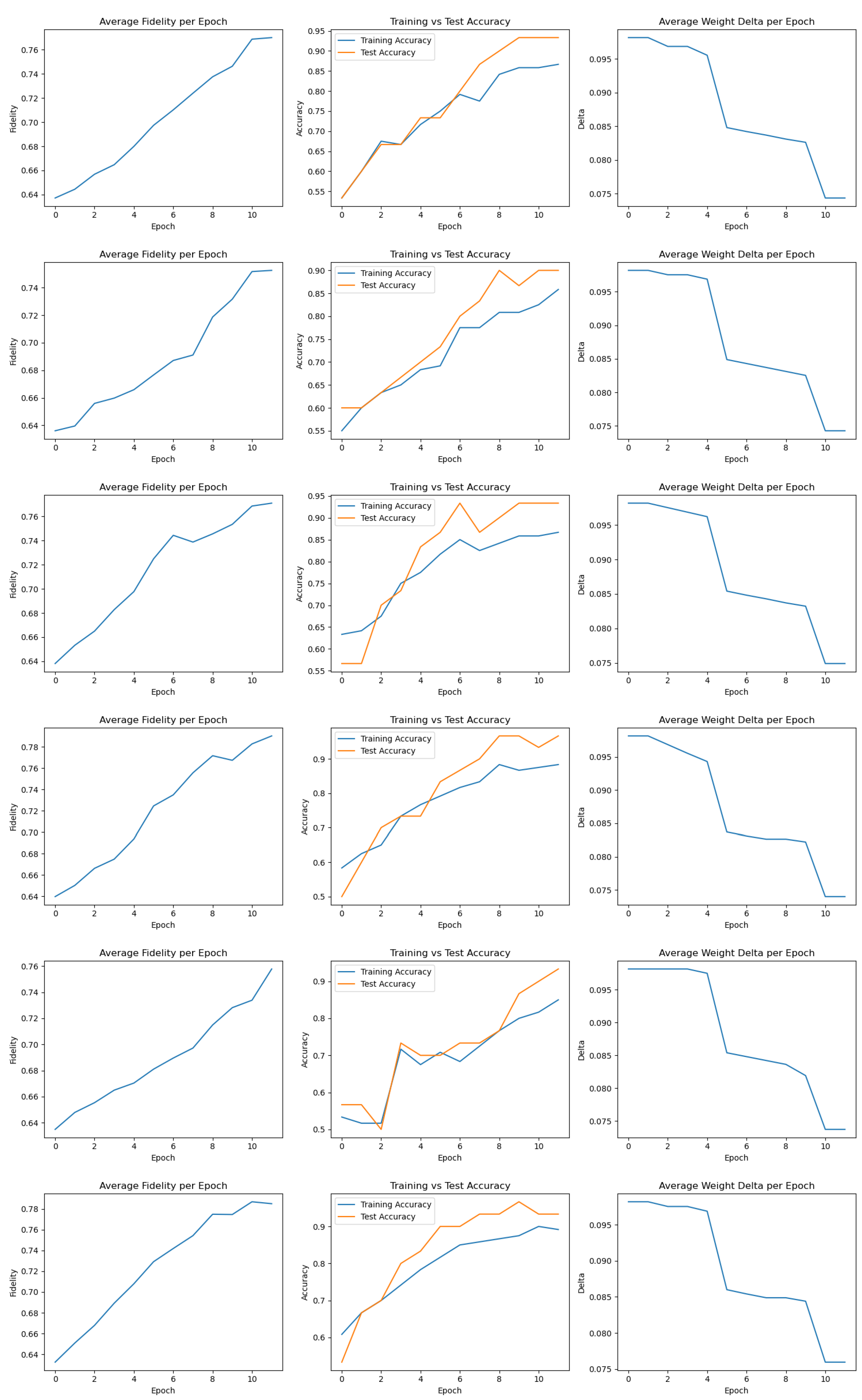
Figure A2.
Training metrics for Runs 7–12.
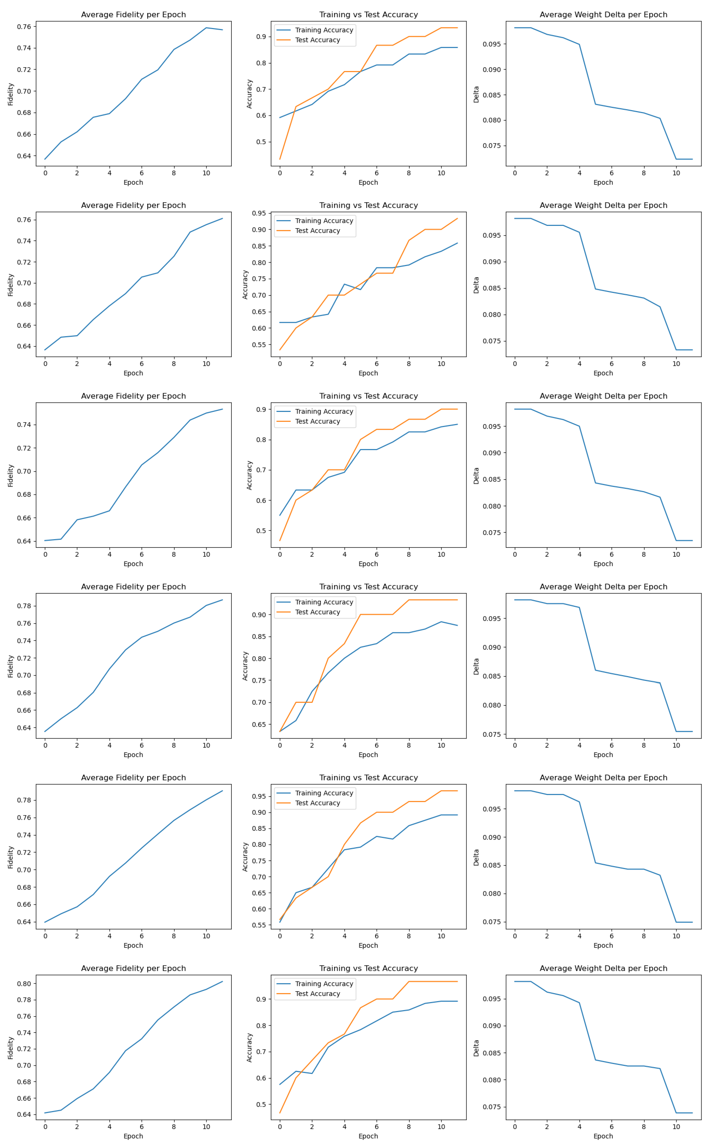
Figure A3.
Training metrics for Runs 13–18.
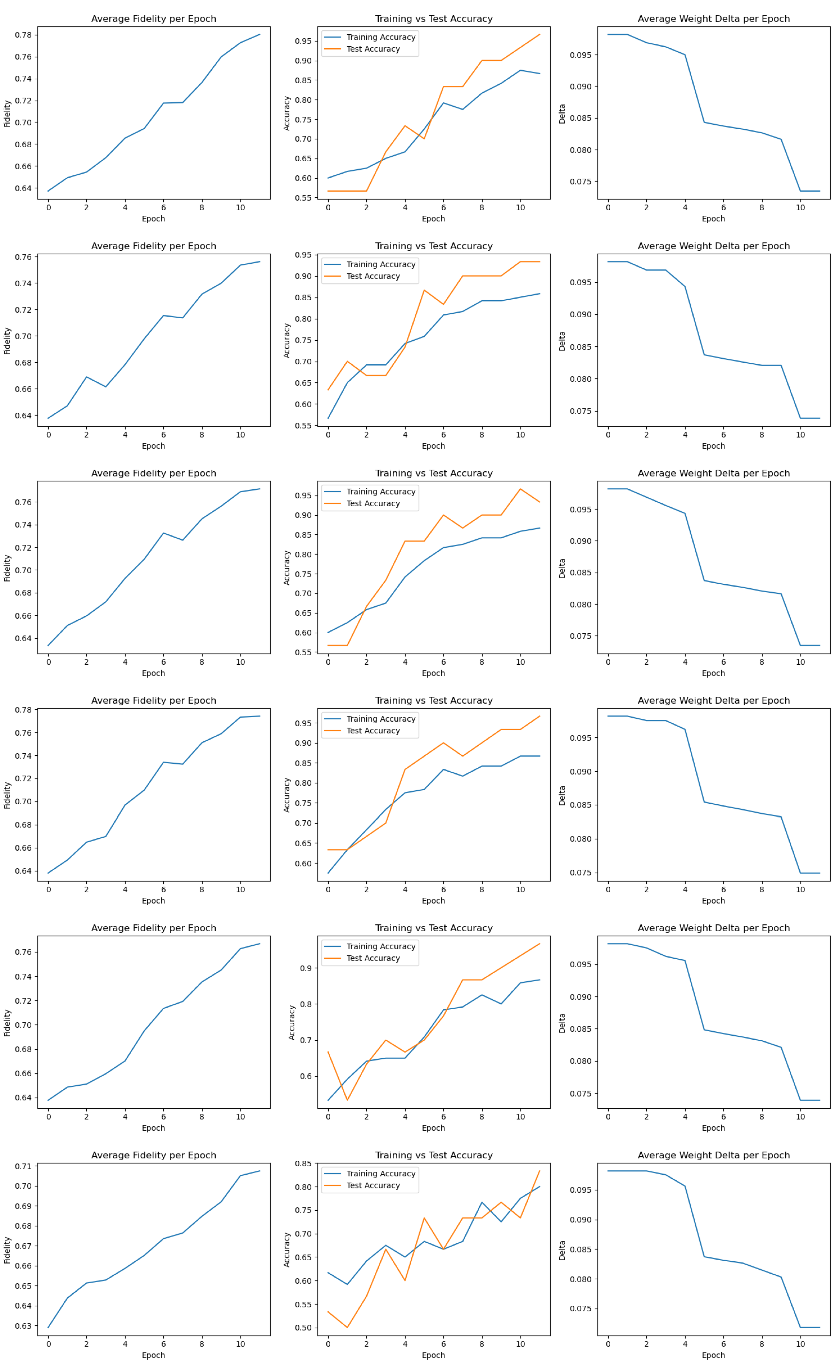
Figure A4.
Training metrics for Runs 19–20.
References
- Wang, Yunfei and Junyu Liu. “A comprehensive review of quantum machine learning: from NISQ to fault tolerance.” Reports on progress in physics. 2024. [CrossRef]
- Zeguendry A, Jarir Z, Quafafou M. Quantum Machine Learning: A Review and Case Studies. Entropy. 2023; 25(2):287. [CrossRef]
- Biamonte, J. , Wittek, P., Pancotti, N. et al. Quantum machine learning. Nature 549, 195–202 (2017). [CrossRef]
- Cerezo, M. , Verdon, G., Huang, HY. et al. Challenges and opportunities in quantum machine learning. Nat Comput Sci 2, 567–576 (2022). [CrossRef]
- Beer, K. , Bondarenko, D., Farrelly, T. et al. Training deep quantum neural networks. Nat Commun 11, 808 (2020). [CrossRef]
- Cui, Wei, and Shilu Yan. “New Directions in Quantum Neural Networks Research — Control Theory and Technology.” SpringerLink, South China University of Technology and Academy of Mathematics and Systems Science, CAS, 6 Nov. 2019, https://link.springer.com/article/10.1007/s11768-019-8289-0.
- Abbas, A. , Sutter, D., Zoufal, C. et al. The power of quantum neural networks. Nat Comput Sci 1, 403–409 (2021). [CrossRef]
- Nielsen, M. A.; Chuang, I. L. (2010). Quantum Computation and Quantum Information: 10th Anniversary Edition. Cambridge: Cambridge University Press.
- Boresta, M.; Colombo, T.; De Santis, A.; et al. A Mixed Finite Differences Scheme for Gradient Approximation. J Optim Theory Appl 194, 1–24 (2022). [CrossRef]
- Author 1, A.B.; Author 2, C. Title of Unpublished Work. Abbreviated Journal Name year, phrase indicating stage of publication (submitted; accepted; in press).
- Title of Site. Available online: URL (accessed on Day Month Year).
- Author 1, A.B.; Author 2, C.D.; Author 3, E.F. Title of presentation. In Proceedings of the Name of the Conference, Location of Conference, Country, Date of Conference (Day Month Year); Abstract Number (optional), Pagination (optional).
- Author 1, A.B. Title of Thesis. Level of Thesis, Degree-Granting University, Location of University, Date of Completion.
Figure 1.
Performance metrics for the best-performing FQNN training run (Run 12). Left: fidelity, center: classification accuracy, right: delta decay.
Figure 1.
Performance metrics for the best-performing FQNN training run (Run 12). Left: fidelity, center: classification accuracy, right: delta decay.
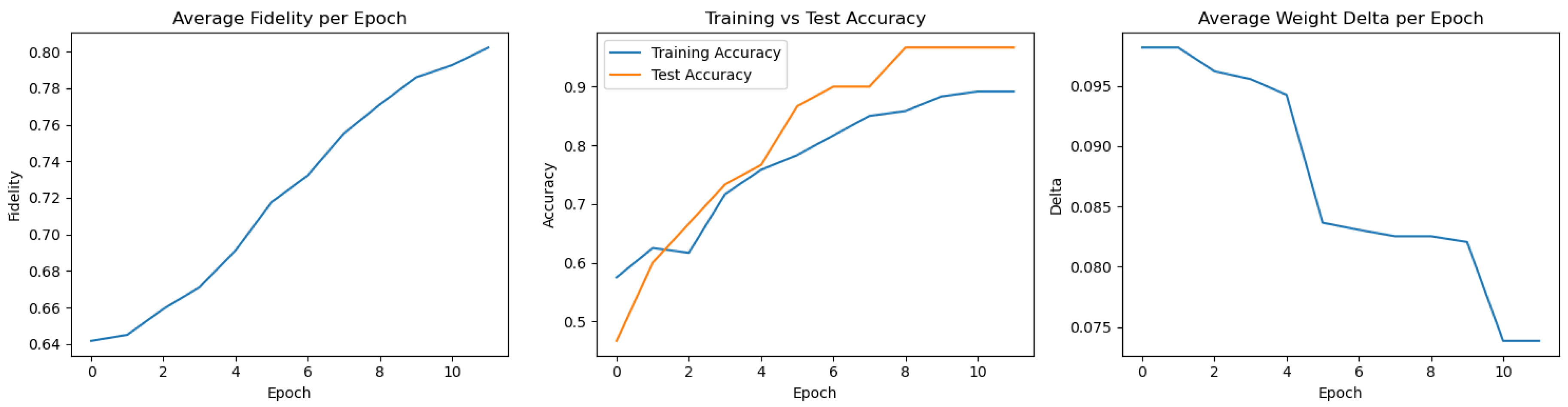
Figure 3.
Average fidelity per epoch across 20 independent FQNN training runs. Each curve represents a single run.
Figure 3.
Average fidelity per epoch across 20 independent FQNN training runs. Each curve represents a single run.
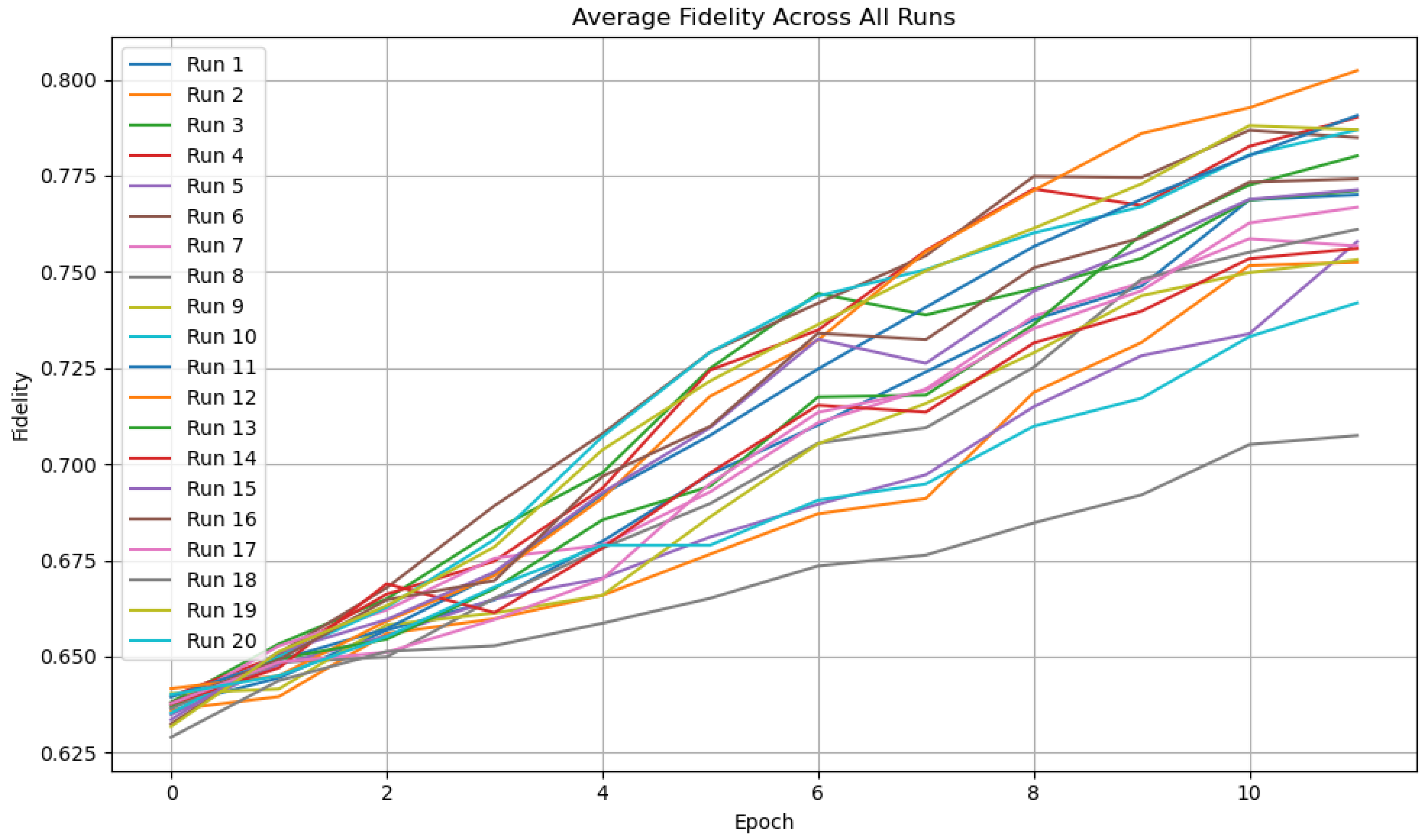
Figure 4.
Test classification accuracy across 20 independent FQNN training runs. Each line represents a separate run over 12 epochs.
Figure 4.
Test classification accuracy across 20 independent FQNN training runs. Each line represents a separate run over 12 epochs.
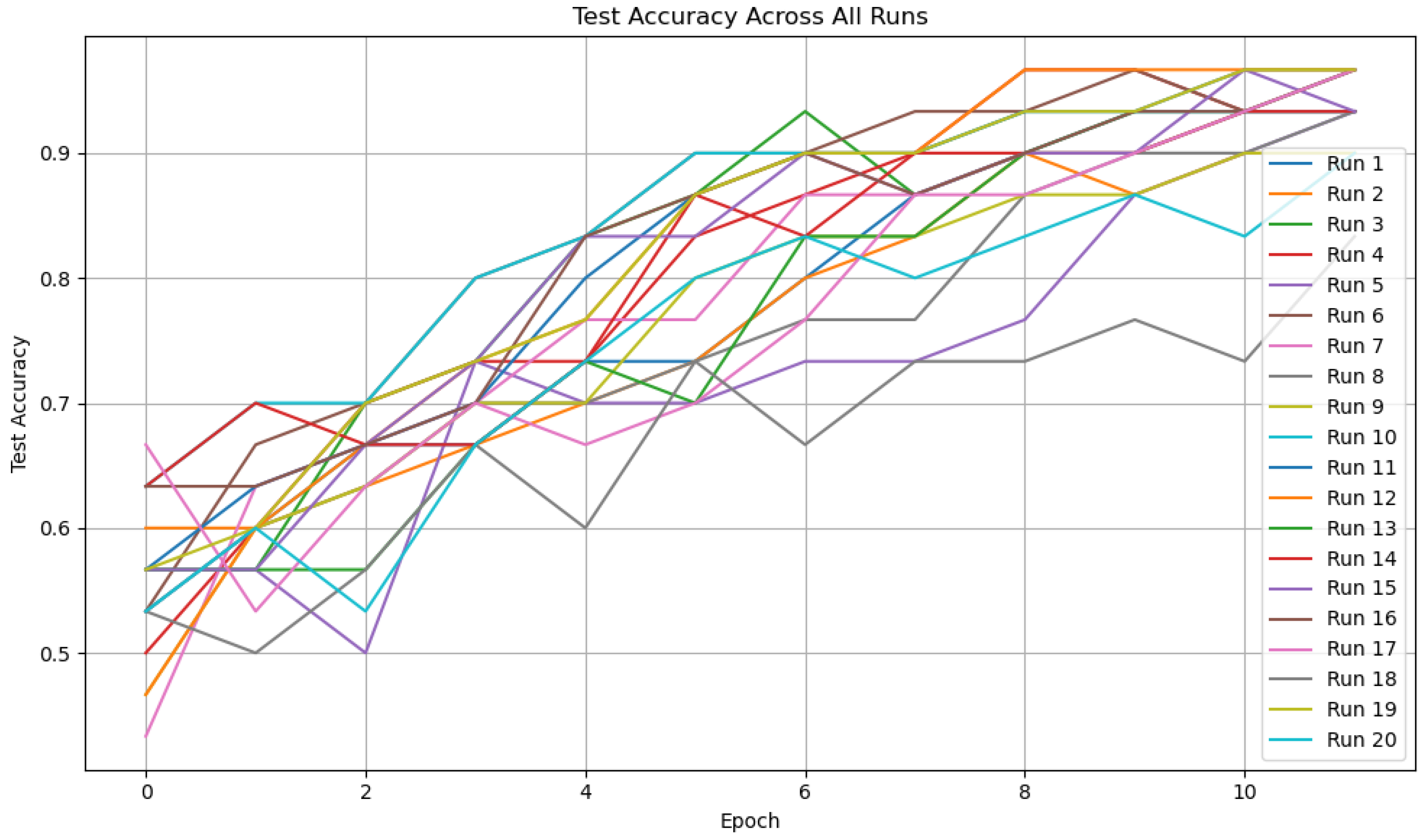

Table 1.
Final test set predictions for the best-performing FQNN run (Run 12).
| Sample # | Input Features (scaled) | Predicted | Expected |
|---|---|---|---|
| 1 | [0.03, 0.42, 0.05, 0.04] | 0 | 0 |
| 2 | [0.50, 0.42, 0.66, 0.71] | 2 | 2 |
| 3 | [0.17, 0.17, 0.39, 0.38] | 1 | 1 |
| 4 | [0.19, 0.12, 0.39, 0.38] | 1 | 1 |
| 5 | [0.03, 0.50, 0.05, 0.04] | 0 | 0 |
| 6 | [0.56, 0.54, 0.63, 0.63] | 1 | 1 |
| 7 | [0.08, 0.67, 0.00, 0.04] | 0 | 0 |
| 8 | [0.31, 0.58, 0.12, 0.04] | 0 | 0 |
| 9 | [0.61, 0.42, 0.71, 0.79] | 2 | 2 |
| 10 | [0.31, 0.42, 0.59, 0.58] | 1 | 1 |
| 11 | [0.83, 0.38, 0.90, 0.71] | 0 | 2 |
| 12 | [0.72, 0.46, 0.69, 0.92] | 2 | 2 |
| 13 | [0.61, 0.42, 0.81, 0.88] | 2 | 2 |
| 14 | [0.58, 0.50, 0.59, 0.58] | 1 | 1 |
| 15 | [0.19, 0.58, 0.08, 0.04] | 0 | 0 |
| 16 | [0.19, 0.54, 0.07, 0.04] | 0 | 0 |
| 17 | [0.42, 0.83, 0.03, 0.04] | 0 | 0 |
| 18 | [0.36, 0.21, 0.49, 0.42] | 1 | 1 |
| 19 | [0.50, 0.38, 0.63, 0.54] | 1 | 1 |
| 20 | [0.47, 0.42, 0.64, 0.71] | 2 | 2 |
| 21 | [0.31, 0.71, 0.08, 0.04] | 0 | 0 |
| 22 | [0.67, 0.46, 0.78, 0.96] | 2 | 2 |
| 23 | [0.64, 0.38, 0.61, 0.50] | 1 | 1 |
| 24 | [0.50, 0.25, 0.78, 0.54] | 2 | 2 |
| 25 | [0.58, 0.33, 0.78, 0.88] | 2 | 2 |
| 26 | [0.67, 0.42, 0.68, 0.67] | 1 | 1 |
| 27 | [0.64, 0.42, 0.58, 0.54] | 1 | 1 |
| 28 | [0.39, 0.75, 0.12, 0.08] | 0 | 0 |
| 29 | [0.61, 0.42, 0.76, 0.71] | 2 | 2 |
| 30 | [0.25, 0.58, 0.07, 0.04] | 0 | 0 |
Table 2.
Final test set predictions for the worst-performing FQNN run (Run 18).
| Sample # | Input Features (scaled) | Predicted | Expected |
|---|---|---|---|
| 1 | [0.03, 0.42, 0.05, 0.04] | 0 | 0 |
| 2 | [0.50, 0.42, 0.66, 0.71] | 2 | 2 |
| 3 | [0.17, 0.17, 0.39, 0.38] | 1 | 1 |
| 4 | [0.19, 0.12, 0.39, 0.38] | 1 | 1 |
| 5 | [0.03, 0.50, 0.05, 0.04] | 0 | 0 |
| 6 | [0.56, 0.54, 0.63, 0.63] | 1 | 1 |
| 7 | [0.08, 0.67, 0.00, 0.04] | 0 | 0 |
| 8 | [0.31, 0.58, 0.12, 0.04] | 0 | 0 |
| 9 | [0.61, 0.42, 0.71, 0.79] | 0 | 2 |
| 10 | [0.31, 0.42, 0.59, 0.58] | 1 | 1 |
| 11 | [0.83, 0.38, 0.90, 0.71] | 0 | 2 |
| 12 | [0.72, 0.46, 0.69, 0.92] | 0 | 2 |
| 13 | [0.61, 0.42, 0.81, 0.88] | 2 | 2 |
| 14 | [0.58, 0.50, 0.59, 0.58] | 1 | 1 |
| 15 | [0.19, 0.58, 0.08, 0.04] | 0 | 0 |
| 16 | [0.19, 0.54, 0.07, 0.04] | 0 | 0 |
| 17 | [0.42, 0.83, 0.03, 0.04] | 0 | 0 |
| 18 | [0.36, 0.21, 0.49, 0.42] | 1 | 1 |
| 19 | [0.50, 0.38, 0.63, 0.54] | 1 | 1 |
| 20 | [0.47, 0.42, 0.64, 0.71] | 2 | 2 |
| 21 | [0.31, 0.71, 0.08, 0.04] | 0 | 0 |
| 22 | [0.67, 0.46, 0.78, 0.96] | 0 | 2 |
| 23 | [0.64, 0.38, 0.61, 0.50] | 1 | 1 |
| 24 | [0.50, 0.25, 0.78, 0.54] | 2 | 2 |
| 25 | [0.58, 0.33, 0.78, 0.88] | 2 | 2 |
| 26 | [0.67, 0.42, 0.68, 0.67] | 1 | 1 |
| 27 | [0.64, 0.42, 0.58, 0.54] | 1 | 1 |
| 28 | [0.39, 0.75, 0.12, 0.08] | 0 | 0 |
| 29 | [0.61, 0.42, 0.76, 0.71] | 0 | 2 |
| 30 | [0.25, 0.58, 0.07, 0.04] | 0 | 0 |
Table 3.
Final classification accuracy on training and test sets for 20 independent FQNN runs.
| Run ID | Training Accuracy | Test Accuracy |
|---|---|---|
| 1 | 0.8667 | 0.9333 |
| 2 | 0.8583 | 0.9000 |
| 3 | 0.8667 | 0.9333 |
| 4 | 0.8833 | 0.9667 |
| 5 | 0.8500 | 0.9333 |
| 6 | 0.8917 | 0.9333 |
| 7 | 0.8583 | 0.9333 |
| 8 | 0.8583 | 0.9333 |
| 9 | 0.8500 | 0.9000 |
| 10 | 0.8750 | 0.9333 |
| 11 | 0.8917 | 0.9667 |
| 12 | 0.8917 | 0.9667 |
| 13 | 0.8667 | 0.9667 |
| 14 | 0.8583 | 0.9333 |
| 15 | 0.8667 | 0.9333 |
| 16 | 0.8667 | 0.9667 |
| 17 | 0.8667 | 0.9667 |
| 18 | 0.8000 | 0.8333 |
| 19 | 0.8750 | 0.9667 |
| 20 | 0.8417 | 0.9000 |
| Mean | 0.8642 | 0.9350 |
| Std Dev | 0.0201 | 0.0324 |
| Variance | 0.000403 | 0.001053 |
Disclaimer/Publisher’s Note: The statements, opinions and data contained in all publications are solely those of the individual author(s) and contributor(s) and not of MDPI and/or the editor(s). MDPI and/or the editor(s) disclaim responsibility for any injury to people or property resulting from any ideas, methods, instructions or products referred to in the content. |
© 2025 by the authors. Licensee MDPI, Basel, Switzerland. This article is an open access article distributed under the terms and conditions of the Creative Commons Attribution (CC BY) license (http://creativecommons.org/licenses/by/4.0/).
Copyright: This open access article is published under a Creative Commons CC BY 4.0 license, which permit the free download, distribution, and reuse, provided that the author and preprint are cited in any reuse.


