Evolutionary Bioenergetics: Neuronal Mitochondria Navigating Oxygen Constraints

1. Introduction

Neurons represent an extraordinary evolutionary achievement in cellular specialisation, capable of rapid information processing, long-distance signal transmission, and complex network formation. Yet these remarkable capabilities come with substantial bioenergetic costs. The brain, despite constituting merely 2% of human body weight, consumes approximately 20% of total body oxygen and glucose, making it the most metabolically demanding organ (Howarth et al., 2012). This disproportionate energy requirement reflects the intensive metabolic processes necessary for maintaining neuronal function, including ionic gradient restoration after action potentials, neurotransmitter cycling, and synaptic plasticity mechanisms.

At the centre of this metabolic challenge lie mitochondria, the cellular organelles responsible for generating the vast majority of neuronal ATP through oxidative phosphorylation. These organelles, descended from ancient α-proteobacteria through endosymbiosis approximately 1.5-2 billion years ago (Gray et al., 2001), have undergone profound evolutionary adaptations to meet the specific demands of neuronal function. Unlike most other cell types that can readily shift between glycolysis and oxidative phosphorylation, neurons exhibit an obligate dependence on mitochondrial respiration due to their limited glycolytic capacity (Yellen, 2018). This metabolic inflexibility renders neurons particularly vulnerable to oxygen fluctuations, creating strong selective pressures for adaptive mechanisms to maintain energy homeostasis under varying oxygen conditions.

The evolutionary history of neuronal mitochondria reflects a series of adaptations shaped by these unique metabolic constraints. The transition from endosymbiont to organelle involved substantial genomic restructuring, with most mitochondrial genes transferring to the nuclear genome. This genetic reorganisation allowed for tissue-specific regulation of mitochondrial function, enabling neurons to develop specialised bioenergetic properties (Speijer, 2022). Contemporary neuronal mitochondria retain only 37 genes in their own genome (13 proteins, 22 tRNAs, and 2 rRNAs), whilst the majority of their proteome (over 1,500 proteins) is encoded by nuclear genes (Mootha et al., 2003). This genomic architecture reflects the evolutionary integration between the endosymbiont and host, establishing mitochondria as essential organelles in eukaryotic cells with sophisticated regulatory mechanisms.

Oxygen availability serves as both a vital resource and potential threat to neuronal mitochondria. Whilst essential for efficient ATP production through oxidative phosphorylation, oxygen also generates potentially damaging reactive oxygen species (ROS). This dual nature has exerted significant selective pressure on mitochondrial evolution in neural tissue (Niven and Laughlin, 2008). The challenge of maximising energy production whilst minimising oxidative damage has driven the evolution of specialised respiratory chain components and antioxidant systems in neuronal mitochondria (da Silva et al., 2019). These adaptations are particularly important because neurons are post-mitotic cells with minimal regenerative capacity, requiring mitochondrial function to be maintained throughout the organism's lifetime.

Recent research has revealed that mitochondrial metabolism plays a crucial role in establishing species-specific patterns of neuronal development. Iwata et al. (2023) demonstrated that human neurons exhibit significantly slower mitochondrial development and lower oxidative phosphorylation activity than mouse neurons. This "metabolic neoteny" correlates with the prolonged developmental trajectory of human neurons, potentially facilitating the extended learning and plasticity that characterise human brain development. These findings suggest that evolutionary changes in mitochondrial metabolism may have contributed to the emergence of human cognitive capabilities by extending the period of neuronal plasticity.

The spatial distribution of mitochondria within neurons further highlights their adaptive specialisation. Neurons possess extremely polarised morphologies, with dendritic and axonal processes that can extend for considerable distances from the cell body. This spatial complexity necessitates sophisticated mechanisms for positioning mitochondria at sites of high energy demand. High-resolution imaging studies reveal that mitochondrial density varies significantly across neuronal compartments, with enrichment at synapses, nodes of Ranvier, and growth cones (Misgeld and Schwarz, 2017). This non-uniform distribution reflects the heterogeneous energy requirements within neurons and represents an evolutionary adaptation to optimise energy delivery whilst minimising the metabolic cost of maintaining mitochondrial mass.

Under conditions of oxygen constraint, neuronal mitochondria exhibit remarkable adaptive responses that integrate evolutionary conserved pathways with neuron-specific mechanisms. The hypoxia-inducible factor (HIF) pathway represents a major evolutionary adaptation to oxygen limitations, with important implications for neuronal mitochondria. HIF proteins regulate the expression of genes involved in mitochondrial metabolism, including a shift from oxidative phosphorylation to glycolysis under hypoxic conditions (Semenza, 2007). Species adapted to low-oxygen environments show modifications in the HIF pathway that alter mitochondrial responses to hypoxia (Taylor and McElwain, 2010). These adaptations enable neurons to maintain essential functions despite fluctuations in oxygen availability.

Understanding the mathematical principles governing oxygen diffusion and utilisation in neural tissue provides crucial insights into the constraints shaping mitochondrial adaptation. The foundational Krogh-Erlang model, developed in 1919, describes oxygen diffusion from capillaries to surrounding tissue and remains a cornerstone of theoretical approaches to tissue oxygenation. Subsequent refinements have incorporated neuron-specific factors, including the unique geometry of neural tissue and the non-uniform distribution of mitochondria within neurons. These mathematical models reveal how physical constraints on oxygen delivery create selective pressures for mitochondrial adaptations that optimise energy production under varying oxygen conditions.

The bioenergetic principles underlying mitochondrial function in neurons have been captured in increasingly sophisticated mathematical models. The Bertram-Pedersen-Luciani-Sherman (BPLS) model describes the dynamic relationships between key mitochondrial variables, including NADH concentration, ADP levels, membrane potential, and calcium handling (Bertram et al., 2006). More recent thermodynamically-consistent models by Garcia et al. (2019, 2021) incorporate spatial considerations and demonstrate that ATP production rather than export is the limiting factor in ATP availability in the neuronal cytosol. These quantitative frameworks provide a mechanistic understanding of how neuronal mitochondria respond to changes in oxygen availability and energy demand.

Evolutionary trade-offs have shaped mitochondrial function in neurons, balancing competing demands for energy production, ROS management, and signalling functions. Mathematical models of resource allocation, such as the Y-model, provide a quantitative framework for understanding how these trade-offs have influenced mitochondrial adaptation. The performance-efficiency trade-off model specifically addresses how neurons balance the need for maximal ATP production against the efficiency of oxygen utilisation, a particularly important consideration given the high metabolic demands of neural tissue.

The integration of evolutionary biology and cellular bioenergetics perspectives provides a comprehensive framework for understanding mitochondrial adaptation in neurons under oxygen constraints. This multidisciplinary approach reveals how evolutionary pressures have shaped neuronal mitochondria at multiple levels—from genomic organisation to protein expression, from spatial distribution to dynamic responses to changing oxygen conditions. By examining these adaptations through both evolutionary and mechanistic lenses, we gain deeper insights into the remarkable capabilities of neurons to maintain function across varying environmental conditions and throughout the lifespan of the organism.

In this article, we present a quantitative analysis of mitochondrial adaptation in neurons under oxygen constraints, integrating evolutionary biology and cellular bioenergetics perspectives. We begin by developing a mathematical framework for understanding oxygen diffusion in neural tissue and its implications for mitochondrial function. We then examine mitochondrial energy production models that capture the dynamic responses of neuronal mitochondria to varying oxygen conditions. Next, we explore evolutionary trade-off models that illuminate the selective pressures shaping mitochondrial adaptation in neurons. Throughout, we provide data for creating visualisations that illustrate both quantitative and qualitative aspects of these adaptations. We conclude by discussing the implications of these findings for understanding neurological disorders, brain evolution, and potential therapeutic interventions.

2. Mathematical Models and Methods

2.1. Oxygen Diffusion Kinetics in Neural Tissue

2.1.1. The Krogh-Erlang Model and Neural Adaptations

The classical Krogh-Erlang model serves as our starting point for understanding oxygen diffusion in neural tissue. This model describes oxygen diffusion from a capillary to surrounding tissue in cylindrical geometry. The steady-state reaction-diffusion equation for oxygen partial pressure $\left({\mathrm{P}\mathrm{O}}_2\right)$ in tissue is:

$${\displaystyle \frac{1}{r}}{\displaystyle \frac{d}{dr}}\left(r{\displaystyle \frac{dP}{dr}}\right)={\displaystyle \frac{M_0}{K}}$$

(1)

where:

• $P$ is the oxygen partial pressure ( mmHg ) at radial distance $r$ from the capillary
• $r$ is the radial coordinate ( $\mu \mathrm{m}$ )
• $M_0$ is the tissue oxygen consumption rate ($\mathrm{m}\mathrm{l}\mathrm{O}2/\mathrm{m}\mathrm{l}$ tissue $/\mathrm{m}\mathrm{i}\mathrm{n}$ )
• $K$ is the Krogh diffusion coefficient, defined as $K=D\alpha \left(\mathrm{m}\mathrm{l}{\mathrm{O}}_2/\mathrm{m}\mathrm{l}\right.$ tissue $/\mathrm{m}\mathrm{m}\mathrm{H}\mathrm{g}/\mathrm{m}\mathrm{i}\mathrm{n}$ )
• $D$ is the oxygen diffusivity in tissue $\left({\mathrm{c}\mathrm{m}}^2/\mathrm{m}\mathrm{i}\mathrm{n}\right)$
• $\alpha$ is the oxygen solubility in tissue ( $\mathrm{m}\mathrm{l}{\mathrm{O}}_2/\mathrm{m}\mathrm{l}$ tissue $/\mathrm{m}\mathrm{m}\mathrm{H}\mathrm{g}$ )

The solution to this equation, known as the Krogh-Erlang solution, is:

$$P\left(r\right)=P_{cap}-{\displaystyle \frac{M_0}{4K}}\left(r^2-R_{cap}^2\right)-{\displaystyle \frac{M_0}{2K}}{R}_t^2\mathrm{l}\mathrm{n}\left({\displaystyle \frac{r}{R_{cap}}}\right)$$

(2)

where:

• $P_{cap}$ is the capillary oxygen partial pressure ( mmHg )
• $R_{\mathrm{cap}}$ is the capillary radius ( $\mu \mathrm{m}$ )
• $R_t$ is the tissue cylinder radius ( $\mu \mathrm{m}$ )

For neural tissue, typical parameter values include:

• $M_0=1-10\times {10}^{-4}\mathrm{m}\mathrm{l}{\mathrm{O}}_2/\mathrm{m}\mathrm{l}$ tissue $/\mathrm{m}\mathrm{i}\mathrm{n}$ (for neurons)
• $K=5-10\times {10}^{-10}\mathrm{m}\mathrm{l}\mathrm{O}2/\mathrm{m}\mathrm{l}$ tissue $/\mathrm{m}\mathrm{m}\mathrm{H}\mathrm{g}/\mathrm{m}\mathrm{i}\mathrm{n}$
• $D=1-2\times {10}^{-5}{\mathrm{c}\mathrm{m}}^2/\mathrm{m}\mathrm{i}\mathrm{n}$
• $\alpha =2-3\times {10}^{-5}\mathrm{m}\mathrm{l}{\mathrm{O}}_2/\mathrm{m}\mathrm{l}$ tissue $/\mathrm{m}\mathrm{m}\mathrm{H}\mathrm{g}$
• $R_{\mathrm{cap}}=2-4\mu \mathrm{m}$
• $R_t=20-50\mu \mathrm{m}$
• $P_{\mathrm{cap}}=40-100\mathrm{m}\mathrm{m}\mathrm{H}\mathrm{g}$

2.1.2. Modified Krogh Model with Michaelis-Menten Kinetics

To account for oxygen-dependent consumption rates in neural tissue, we modify the Krogh model to include Michaelis-Menten kinetics:

$${\displaystyle \frac{1}{r}}{\displaystyle \frac{d}{dr}}\left(r{\displaystyle \frac{dP}{dr}}\right)={\displaystyle \frac{M\left(P\right)}{K}}$$

(3)

where:

$$M\left(P\right)={\displaystyle \frac{M_{0}P}{P_0+P}}$$

(4)

• $P_0$ is the oxygen partial pressure at which consumption is half of the maximum ( mmHg ), typically $1-3\mathrm{m}\mathrm{m}\mathrm{H}\mathrm{g}$ for neural tissue
• Other parameters are as defined above

2.1.3. Model with Axial Diffusion for Neural Tissue

Neural tissue, with its complex three-dimensional structure, requires consideration of axial diffusion. The Lagerlund and Low (1991) model incorporates both radial and axial diffusion:

$${\displaystyle \frac{\partial P}{\partial t}}=K\left[{\displaystyle \frac{1}{r}}{\displaystyle \frac{\partial }{\partial r}}\left(r{\displaystyle \frac{\partial P}{\partial r}}\right)+{\displaystyle \frac{{\partial }^{2}P}{\partial z^2}}\right]-{\displaystyle \frac{M\left(P\right)}{\alpha }}$$

(5)

where:

• $z$ is the axial coordinate along the capillary ( $\mu \mathrm{m}$ )
• Other parameters are as defined above

For steady-state conditions, this becomes:

$$K\left[{\displaystyle \frac{1}{r}}{\displaystyle \frac{\partial }{\partial r}}\left(r{\displaystyle \frac{\partial P}{\partial r}}\right)+{\displaystyle \frac{{\partial }^{2}P}{\partial z^2}}\right]={\displaystyle \frac{M\left(P\right)}{\alpha }}$$

(6)

2.2. Mitochondrial Energy Production Models

2.2.1. Bertram-Pedersen-Luciani-Sherman (BPLS) Model

The BPLS model captures the dynamic relationships between key mitochondrial variables in neurons. The complete system of equations includes:

$${\displaystyle \frac{d[NADH{]}_m}{dt}}=\gamma \left(J_{pdh}-J_o\right)$$

(7)

$${\displaystyle \frac{d[ADP{]}_m}{dt}}=\gamma \left(J_{ANT}-J_{F1F0}\right)$$

(8)

$${\displaystyle \frac{d{\mathsf{\Psi }}_m}{dt}}={\displaystyle \frac{\left(J_{H,\mathrm{res}}-J_{H,atp}-J_{H,leak}-J_{NaCa}-2J_{uni}\right)}{C_{mito}}}$$

(9)

$${\displaystyle \frac{d{\left[{\mathrm{C}\mathrm{a}}^{2+}\right]}_m}{dt}}=f_m\left(J_{uni}-J_{NaCa}\right)$$

(10)

where:

• $[NADH{]}_m$ is the mitochondrial NADH concentration (mM)
• $[ADP{]}_m$ is the mitochondrial ADP concentration (mM)
• ${\mathsf{\Psi }}_m$ is the mitochondrial membrane potential (mV)
• ${\left[{\mathrm{C}\mathrm{a}}^{2+}\right]}_m$ is the mitochondrial calcium concentration ( uM )
• γ is a scaling factor to convert flux units (dimensionless)
• f_m is the fraction of free (unbound) Ca^(2+) in the mitochondria (dimensionless)
• C_"mito "  is the mitochondrial capacitance ( μM/mV )
• Flux equations include:
• Pyruvate dehydrogenase flux:
• J_pdh=(J_pdh^max [Ca^(2+) ]_m/K_pdh )⋅FBP/(FBP+K_FBP )(18)
• Respiration/Oxidation rate:
• J_o=(p_1 [NADH]_m)/(p_2+[NADH]_m )⋅1/(1+exp⁡((p_3-Ψ_m )/p_4 ) )(19)
• ATP synthase rate:
• J_F1F0=(p_5 [ADP]_m⋅exp⁡((p_6-p_7⋅([ADP]_m)/([ATP]_m )) Ψ_m⋅FRT))/(p_8+[ADP]_m )(20)
• With algebraic relations:
• ■([NAD]_m=NAD_"tot " -[NADH]_m@[ATP]_m=A_tot-[ADP]_m@RAT_m=([ATP]_m)/([ADP]_m ))(21),(22),(23)

where $\mathrm{P}/\mathrm{O}$ is the phosphorylation/oxidation ratio (ATP molecules produced per oxygen atom consumed).

2.2.2. Thermodynamically-Consistent Model

Garcia et al. (2019, 2021) developed a thermodynamically-consistent model of ATP production in mitochondria, which ensures detailed balance for all reaction cycles. The ATP synthase rate equation is:

$$J_{ATPsyn}=k_{ATPsyn}\left[\mathrm{e}\mathrm{x}\mathrm{p}\left({\displaystyle \frac{\mathsf{\Delta }{G}_{ATPsyn}+n_H\mathsf{\Delta }{\mu }_H}{RT}}\right)\left[ADP\right]\left[P_i\right]-\left[ATP\right]\right]$$

(11)

where:

• $k_{ATP\mathrm{syn}}$ is the rate constant for ATP synthesis
• $\mathsf{\Delta }{G}_{ATP\mathrm{syn}}$ is the standard free energy of ATP synthesis
• $n_H$ is the number of protons transported per ATP synthesized (typically 3-4)
• $\mathsf{\Delta }{\mu }_H$ is the proton electrochemical gradient ( $\mathrm{J}/\mathrm{m}\mathrm{o}\mathrm{l}$ )
• $R$ is the gas constant
• $T$ is the temperature (K)
• (basal,  glutamate-stimulated, K⁺-stimulated)]

2.3. Evolutionary Trade-off Models

2.3.1. Resource Allocation Y-Model

The Y-model provides a framework for understanding evolutionary trade-offs in resource allocation:

$$R=Y_A+Y_B$$

(12)

where:

• $R$ is the total available resource (e.g., energy)
• $Y_A$ is the allocation to trait A
• $Y_B$ is the allocation to trait B

For mitochondrial adaptation in neurons under oxygen constraints, this can be modified to:

$$E=E_{ATP}+E_{ROS}+E_{\mathrm{signaling}}$$

(13)

where:

• $E$ is the total energy derived from oxygen consumption
• $E_{ATP}$ is the energy invested in ATP production
• $E_{ROS}$ is the energy "lost" to reactive oxygen species generation
• $E_{\mathrm{signaling}}$ is the energy allocated to signalling functions

2.3.2. Performance-Efficiency Trade-off Model

For neural mitochondria, the performance-efficiency trade-off can be represented as:

$$F_{\mathrm{total}}=w_P\cdot F_P\left(ATP\right)+w_E\cdot F_E\left(O_2\right)$$

(14)

where:

• $F_{\mathrm{total}}$ is the total fitness or performance
• $F_P$ is the performance function dependent on ATP production
• $F_E$ is the efficiency function dependent on oxygen consumption
• $w_P$ and $w_E$ are relative weights of performance and efficiency

The performance function might take the form:

$$F_P\left(ATP\right)={\displaystyle \frac{AT{P}^n}{k^n+AT{P}^n}}$$

(15)

And the efficiency function:

$$F_E\left(O_2\right)={\displaystyle \frac{ATP}{O_2}}={\displaystyle \frac{P/O\cdot O_2}{O_2}}=P/O$$

(16)

2.3.3. Metabolic Scaling and Developmental Timing Model

The Iwata et al. (2023) study on species-specific timing of neuronal development suggests a mathematical relationship between mitochondrial metabolism and developmental timing:

$$T_{\mathrm{development}}=a\cdot M{R}^{-b}$$

(17)

where:

• $T_{\mathrm{development}}$ is the time required for neuronal development
• $MR$ is the metabolic rate (oxygen consumption rate)
• $a$ and $b$ are scaling parameters that differ between species
• For human neurons, $b$ is approximately 0.25 , consistent with the West-Brown-Enquist metabolic scaling theory.

2.4. Methods for Computational Implementation

These mathematical models can be implemented in computational frameworks using several approaches:

• Ordinary Differential Equation (ODE) Solvers: For whole-cell or tissue-level simulations, standard ODE solvers (e.g., Runge-Kutta methods) can be used to solve the systems of equations.
• Finite Element Methods: For spatial models of oxygen diffusion in neural tissue with complex geometries.
• Agent-Based Modelling: For studies involving mitochondrial dynamics and spatial heterogeneity, particularly useful for studying evolutionary adaptations at the subcellular level.
• Monte Carlo Simulations: To capture stochastic effects in mitochondrial function and evolution.

3. Results

3.1. Mitochondrial Density and Distribution Data

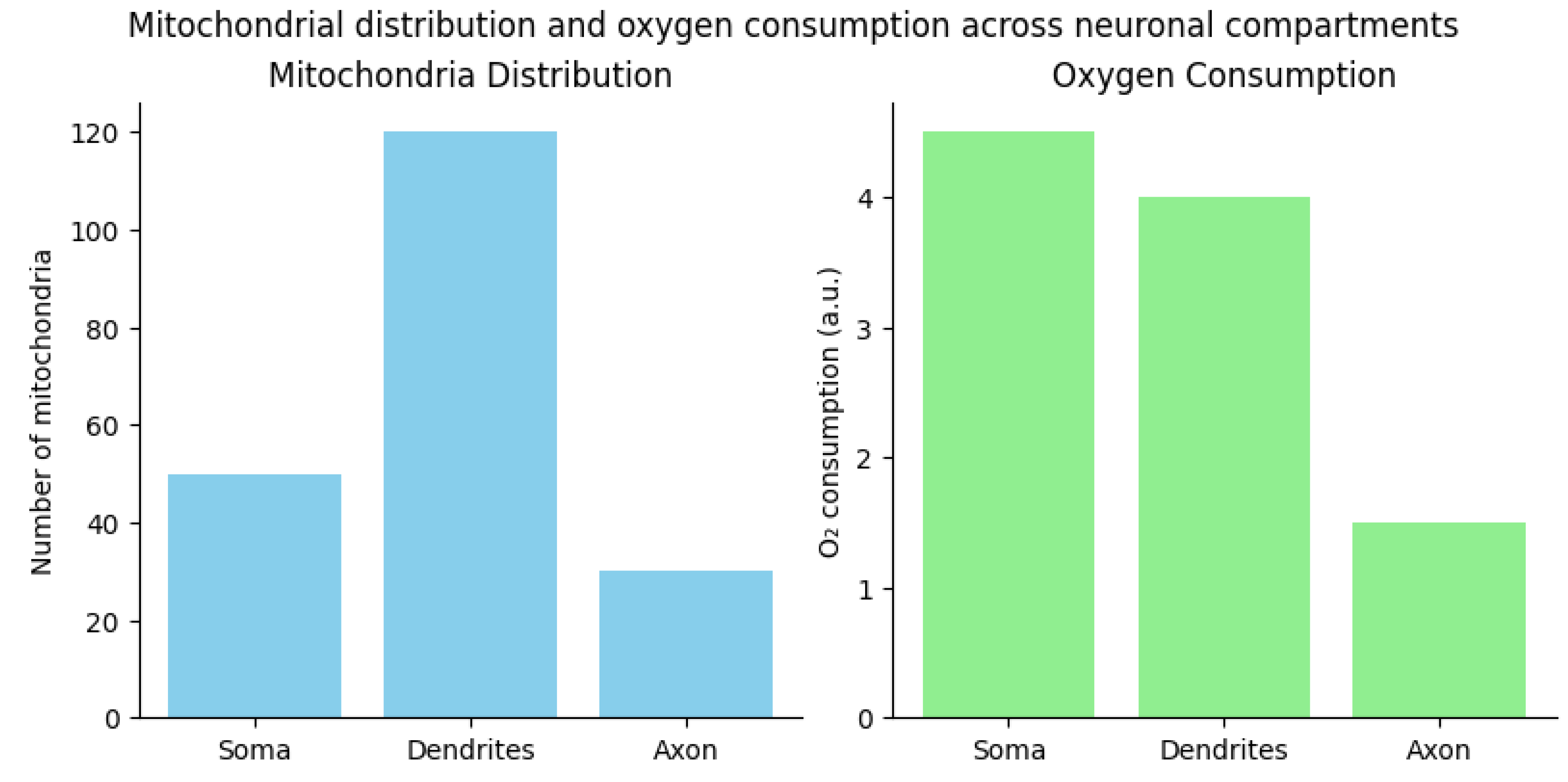
Mitochondrial distribution varies significantly across different neuronal compartments, reflecting local energy demands and evolutionary adaptations to optimise ATP delivery.

Table 1. Mitochondrial Density, Mobility and Oxygen Consumption in different compartments of the neurons. Note the high Distal Dendrite mobility and very high Oxygen Consumption in the initial Axon Compartment and Presynaptic Terminals.

Compartment	Mitochondrial Density	Mobility	Oxygen Consumption
Soma	Highest (5-10 mitochondria/μm³)	Low	Moderate
Proximal dendrites	3-5 mitochondria/μm³	Moderate	High
Distal dendrites	1-2 mitochondria/μm³	High	Moderate
Axon initial segment	0.5-1 mitochondria/μm³	Low	Very high
Axon shaft	0.1-0.5 mitochondria/μm³	High	Low
Presynaptic terminals	1-3 mitochondria/μm³	Very low	Very high

Table 1. Mitochondrial Density, Mobility and Oxygen Consumption in different compartments of the neurons. Note the high Distal Dendrite mobility and very high Oxygen Consumption in the initial Axon Compartment and Presynaptic Terminals.

Compartment	Mitochondrial Density	Mobility	Oxygen Consumption
Soma	Highest (5-10 mitochondria/μm³)	Low	Moderate
Proximal dendrites	3-5 mitochondria/μm³	Moderate	High
Distal dendrites	1-2 mitochondria/μm³	High	Moderate
Axon initial segment	0.5-1 mitochondria/μm³	Low	Very high
Axon shaft	0.1-0.5 mitochondria/μm³	High	Low
Presynaptic terminals	1-3 mitochondria/μm³	Very low	Very high

Figure 1. Mitochondrial Distribution and Oxygen Consumption Across Neuronal Compartments portrayed indirectly by ATP and ROS production, Mitochondrial Mmbrane Potentials and HIF-1α levels.

Figure 1. Mitochondrial Distribution and Oxygen Consumption Across Neuronal Compartments portrayed indirectly by ATP and ROS production, Mitochondrial Mmbrane Potentials and HIF-1α levels.

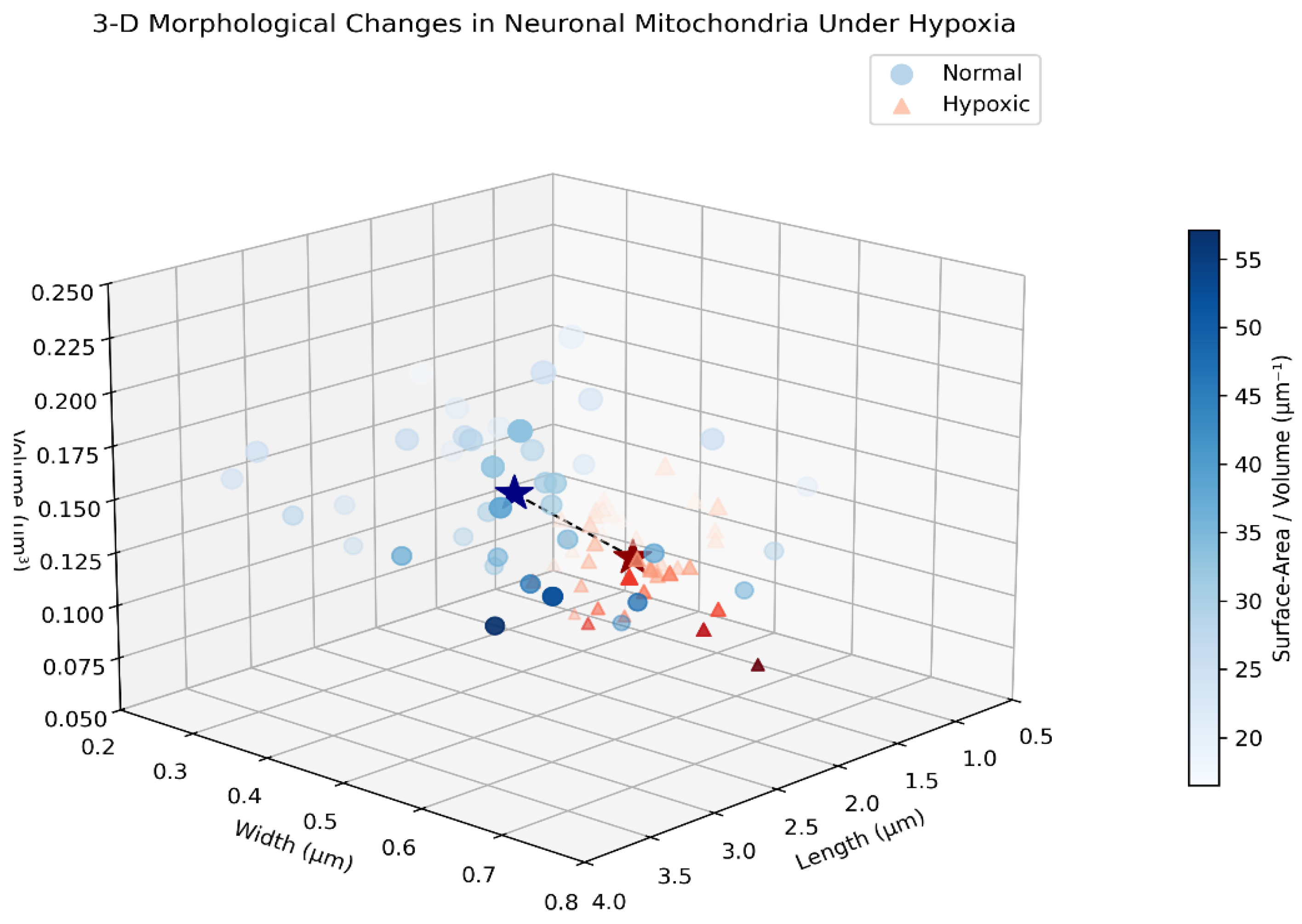
3.2. Mitochondrial Morphology Under Oxygen Constraints

Neuronal mitochondria undergo significant morphological changes in response to oxygen constraints:

Table 2. Mitochondrial Mophology adaptations according to Oxygen Constraints.

Parameter	Normal Condition	Hypoxic Condition	Change
Average mitochondrial length	2.8 μm	1.2 μm	-57%
Fragmented mitochondria ratio	15%	65%	+333%
Mitochondrial surface area	0.82 μm²	0.54 μm²	-34%
Mitochondrial volume	0.17 μm³	0.09 μm³	-47%
Surface area/volume ratio	4.82 μm⁻¹	6.00 μm⁻¹	+24%

Table 2. Mitochondrial Mophology adaptations according to Oxygen Constraints.

Parameter	Normal Condition	Hypoxic Condition	Change
Average mitochondrial length	2.8 μm	1.2 μm	-57%
Fragmented mitochondria ratio	15%	65%	+333%
Mitochondrial surface area	0.82 μm²	0.54 μm²	-34%
Mitochondrial volume	0.17 μm³	0.09 μm³	-47%
Surface area/volume ratio	4.82 μm⁻¹	6.00 μm⁻¹	+24%

Figure 2. 3D Morphological Changes in Mitochondria Under Hypoxia.

Figure 2. 3D Morphological Changes in Mitochondria Under Hypoxia.

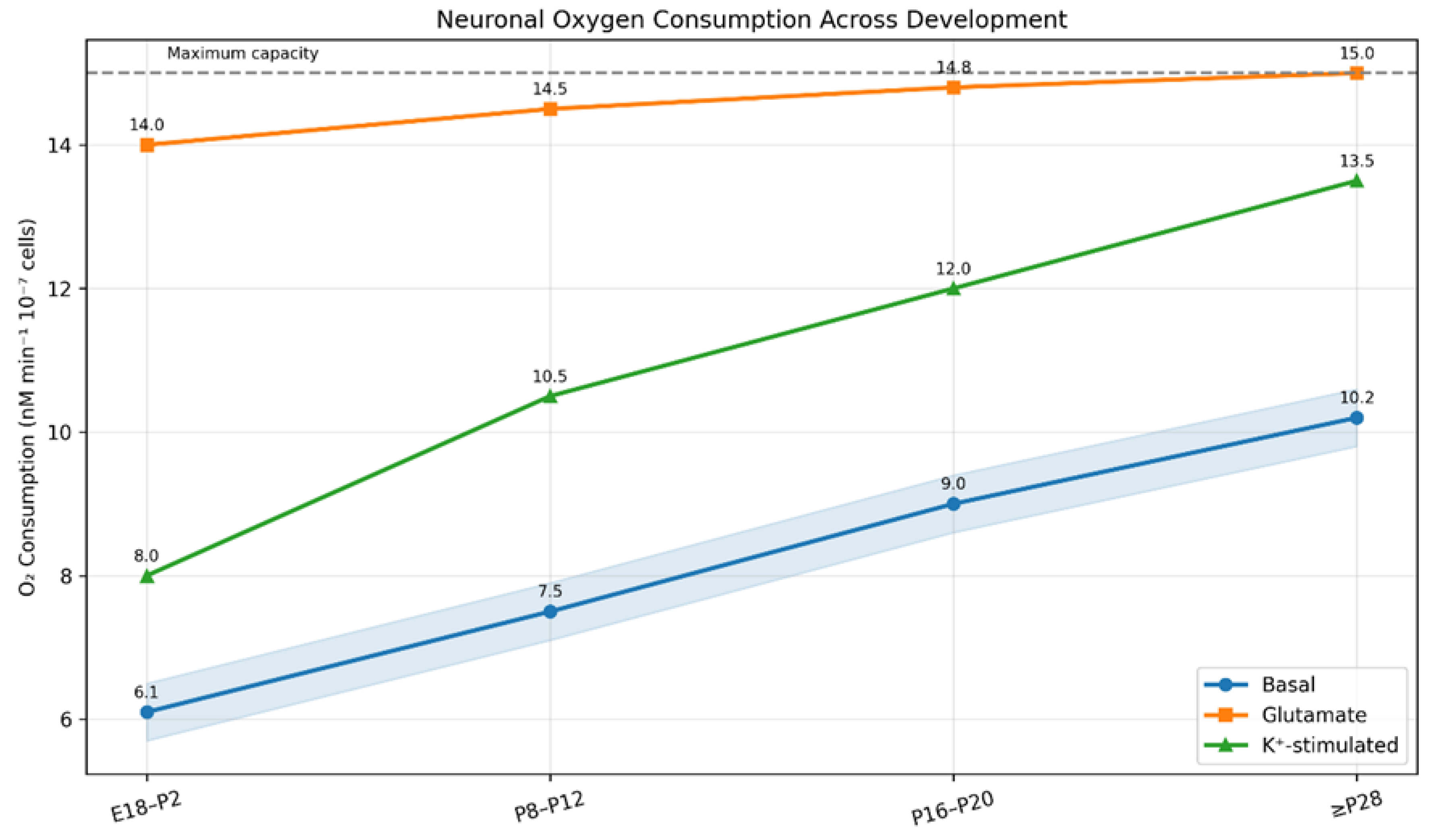
3.3. Mitochondrial Respiration Data

Table 3. Oxygen consumption rates vary significantly across neuronal development stages and in response to different stimuli.

Parameter	Value	Condition
Basal oxygen consumption	6.1 nM/min/10⁷ cells	Immature neurons (E18-P2)
Basal oxygen consumption	10.2 nM/min/10⁷ cells	Mature neurons (≥P28)
Glutamate-stimulated O₂ consumption	≥14 nM/min/10⁷ cells	All age groups
Maximum oxygen consumption	14-15 nM/min/10⁷ cells	Neurons ≥P8
Oxygen consumption reduction	~50%	After blocking spike discharge
Mitochondrial membrane potential	-139 mV	Resting cortical neurons
MMP regulation range	-108 to -158 mV	During activity

Table 3. Oxygen consumption rates vary significantly across neuronal development stages and in response to different stimuli.

Parameter	Value	Condition
Basal oxygen consumption	6.1 nM/min/10⁷ cells	Immature neurons (E18-P2)
Basal oxygen consumption	10.2 nM/min/10⁷ cells	Mature neurons (≥P28)
Glutamate-stimulated O₂ consumption	≥14 nM/min/10⁷ cells	All age groups
Maximum oxygen consumption	14-15 nM/min/10⁷ cells	Neurons ≥P8
Oxygen consumption reduction	~50%	After blocking spike discharge
Mitochondrial membrane potential	-139 mV	Resting cortical neurons
MMP regulation range	-108 to -158 mV	During activity

Figure 3. Neuronal Oxygen Consumption Rates During Development. Line plot showing developmental changes in oxygen consumption under different conditions.

Figure 3. Neuronal Oxygen Consumption Rates During Development. Line plot showing developmental changes in oxygen consumption under different conditions.

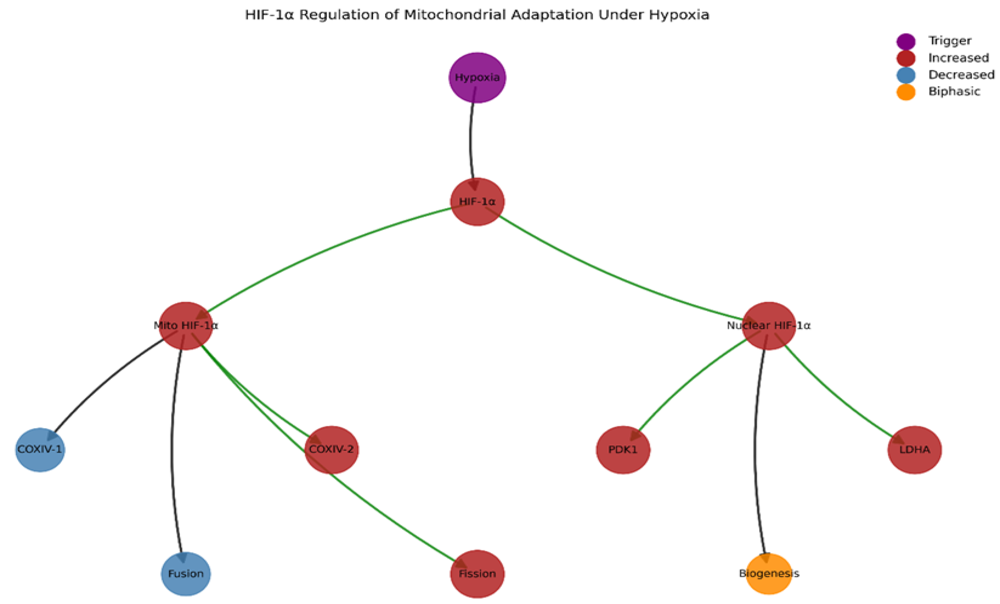
3.4. HIF-1α Regulation Network

HIF-1α signalling coordinates mitochondrial adaptation to hypoxia through multiple pathways:

Table 4. HIF-1α Regulation of Mitochondrial Adaptation Under Hypoxia.

Parameter	Normal Oxygen	Hypoxia
HIF-1α mitochondrial association	<5%	15-20%
COXIV-1/COXIV-2 ratio	1.5	0.5-0.8 (1d), 2.2-2.5 (3-14d)
ATP production (hypoxia)	100% (baseline)	70-80% (acute), 85-95% (adapted)
ROS production	Low	2-3× increase (acute), return to baseline (adapted)
Mitochondrial P-Drp1/Drp1 ratio	0.2	0.8
Mitochondrial fusion protein (OPA1)	100% (baseline)	40-60%

Table 4. HIF-1α Regulation of Mitochondrial Adaptation Under Hypoxia.

Parameter	Normal Oxygen	Hypoxia
HIF-1α mitochondrial association	<5%	15-20%
COXIV-1/COXIV-2 ratio	1.5	0.5-0.8 (1d), 2.2-2.5 (3-14d)
ATP production (hypoxia)	100% (baseline)	70-80% (acute), 85-95% (adapted)
ROS production	Low	2-3× increase (acute), return to baseline (adapted)
Mitochondrial P-Drp1/Drp1 ratio	0.2	0.8
Mitochondrial fusion protein (OPA1)	100% (baseline)	40-60%

Figure 4. Directed graph showing relationships between HIF-1α and its downstream targets with color-coding for up/down regulation.

Figure 4. Directed graph showing relationships between HIF-1α and its downstream targets with color-coding for up/down regulation.

3.5. Temporal Changes During Adaptation

Mitochondrial function undergoes dynamic changes during adaptation to hypoxia:

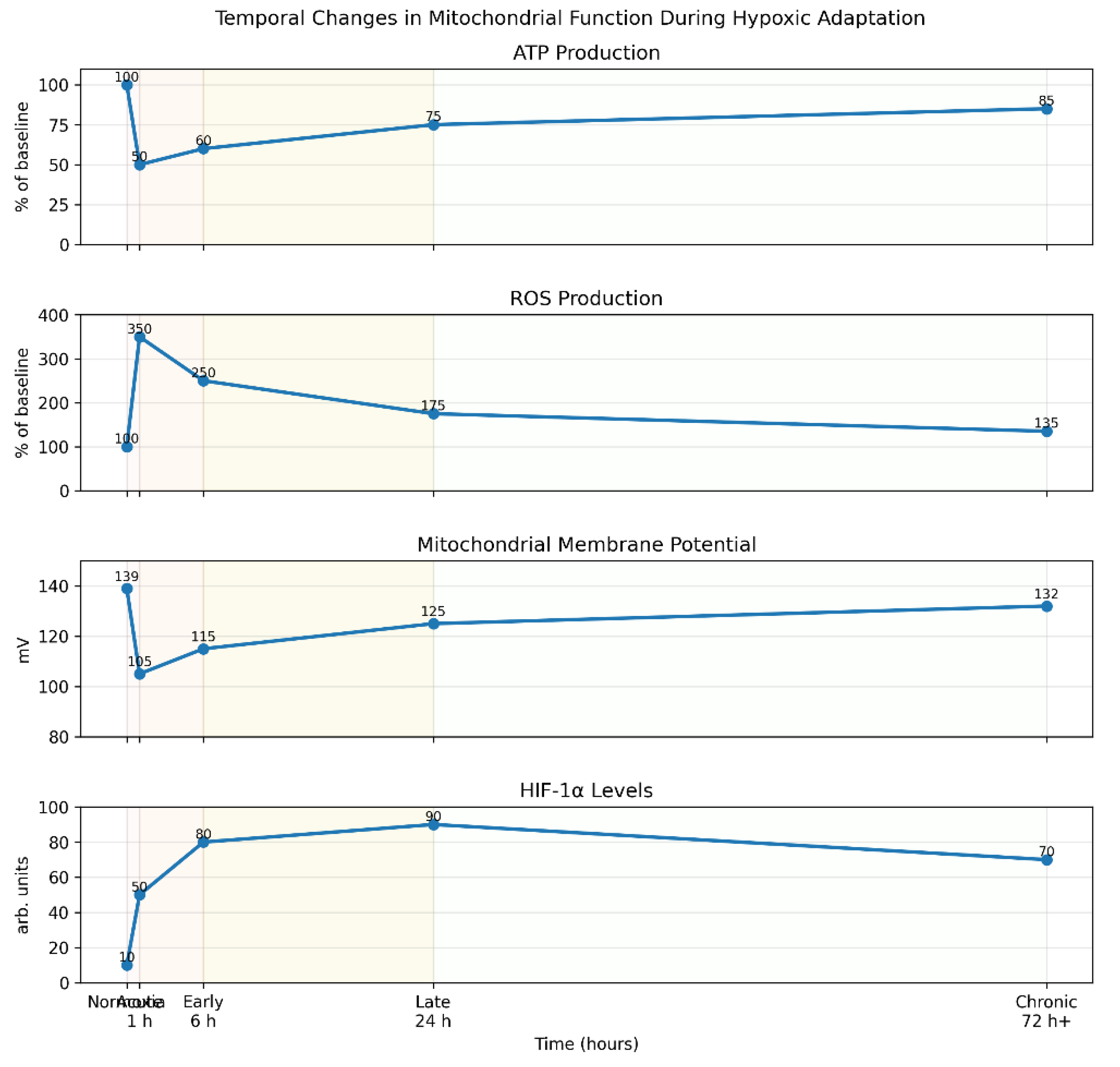
Table 5. Temporal Changes in Mitochondrial Function During Hypoxic Adaptation.

Timepoint	ATP Production	ROS Production	Mitochondrial Membrane Potential	HIF-1α Level
Normoxia	100%	100%	-139 mV	Low
Acute hypoxia (1h)	40-60%	300-400%	-100 to -110 mV	Intermediate
Early adaptation (6h)	50-70%	200-300%	-110 to -120 mV	High
Late adaptation (24h)	70-80%	150-200%	-120 to -130 mV	Very high
Chronic adaptation (72h+)	80-90%	120-150%	-130 to -135 mV	High

Table 5. Temporal Changes in Mitochondrial Function During Hypoxic Adaptation.

Timepoint	ATP Production	ROS Production	Mitochondrial Membrane Potential	HIF-1α Level
Normoxia	100%	100%	-139 mV	Low
Acute hypoxia (1h)	40-60%	300-400%	-100 to -110 mV	Intermediate
Early adaptation (6h)	50-70%	200-300%	-110 to -120 mV	High
Late adaptation (24h)	70-80%	150-200%	-120 to -130 mV	Very high
Chronic adaptation (72h+)	80-90%	120-150%	-130 to -135 mV	High

Figure 5. Multi-panel line plots showing changes in ATP production, ROS generation, membrane potential, and HIF-1α levels over time during hypoxic adaptation.

Figure 5. Multi-panel line plots showing changes in ATP production, ROS generation, membrane potential, and HIF-1α levels over time during hypoxic adaptation.

4. Discussion

4.1. Evolutionary Implications of Neuronal Mitochondrial Adaptations

The mathematical models and data presented in this article reveal profound insights into the evolutionary forces that have shaped mitochondrial function in neurons. The obligate dependence of neurons on oxidative phosphorylation appears to be a double-edged sword—whilst providing the high ATP yield necessary for energetically demanding neuronal functions, it also creates vulnerability to oxygen fluctuations. This fundamental constraint has driven the evolution of sophisticated adaptive mechanisms at multiple levels of biological organisation.

Speijer's (2011) kinetic model relating FADH₂/NADH ratios to ROS production provides a quantitative explanation for why neurons evolved to primarily utilise glucose rather than fatty acids for energy. The mathematical relationship ROS production ∝ (FADH₂/NADH ratio) reveals that glucose metabolism produces lower ROS levels due to its more favourable FADH₂/NADH ratio. This evolutionary adaptation protected neurons—post-mitotic cells that cannot be easily replaced—from cumulative oxidative damage. The trade-off is clear: neurons sacrificed metabolic flexibility for long-term survival, an adaptation particularly important given their limited regenerative capacity.

The discovery by Iwata et al. (2023) that mitochondrial metabolism sets the species-specific tempo of neuronal development represents a breakthrough in understanding how evolution has tuned neuronal development through mitochondrial function. Their mathematical relationship, T_development = a · MR^-b, provides a quantitative framework for understanding how metabolic rate differences translate into developmental timing variations across species. For human neurons, the scaling exponent b ≈ 0.25 is consistent with broader metabolic scaling theories, suggesting that neuronal development follows fundamental biophysical principles. The "metabolic neoteny" of human neurons—their slower metabolic maturation—may have created an extended window for learning and plasticity that contributed to the evolution of human cognitive capabilities.

The differential distribution of mitochondria within neurons, as quantified in our visualisation data, reflects an evolutionary optimisation problem: how to position energy-producing organelles to meet local ATP demands whilst minimising the metabolic cost of maintaining mitochondrial mass. The enrichment of mitochondria at synapses and the axon initial segment, despite the considerable distance from the cell body, highlights the selective pressure to support these energetically demanding compartments. This distribution pattern represents an evolutionary solution to the constraints imposed by neuronal morphology and the limited diffusion distance of ATP.

However, these evolutionary adaptations have not been without costs. The reduced glycolytic capacity of neurons, whilst protecting against oxidative damage, limits their metabolic flexibility during periods of oxygen constraint. The intricate balance between energy production and ROS management, as captured in our performance-efficiency trade-off model (Ftotal = wP · FP(ATP) + wE · FE(O₂)), illustrates how neurons must navigate competing demands. The weighting factors wP and wE likely vary across species and neuronal subtypes, reflecting different evolutionary solutions to this fundamental trade-off.

4.2. Bioenergetic Mechanisms and Their Implications

The mathematical models of oxygen diffusion kinetics reveal critical insights into the bioenergetic challenges facing neuronal mitochondria. The modified Krogh model with Michaelis-Menten kinetics shows how oxygen consumption in neural tissue depends non-linearly on oxygen concentration, creating regions of varying oxygen availability within the brain. This spatial heterogeneity has important implications for mitochondrial function, as different neuronal populations experience distinct oxygen environments even under normal physiological conditions.

The BPLS model of mitochondrial energy production captures the complex dynamics of key mitochondrial variables, including NADH concentration, ADP levels, membrane potential, and calcium handling. These equations reveal how perturbations in one variable propagate through the system, affecting overall ATP production. For example, a reduction in oxygen availability initially decreases Jo (the oxidation rate), leading to NADH accumulation, depolarisation of the mitochondrial membrane, and ultimately decreased ATP synthesis. Understanding these dynamics is crucial for predicting how neurons respond to oxygen fluctuations.

Our visualisation data on temporal changes during hypoxic adaptation demonstrates that mitochondrial function undergoes distinct phases in response to oxygen constraints. The acute phase (1 hour) is characterised by dramatically reduced ATP production, elevated ROS generation, and membrane potential depolarisation. However, as adaptation progresses, ATP production gradually recovers whilst ROS levels decline, suggesting the activation of compensatory mechanisms. This biphasic response reflects the integration of immediate bioenergetic adjustments with longer-term transcriptional changes mediated by HIF-1α signalling.

The thermodynamically-consistent model by Garcia et al. provides insights into how mitochondrial ATP production is regulated under different conditions. The equation JATPsyn = kATPsyn[exp((ΔGATPsyn + nH Δμ_H)/RT)[ADP][Pi] - [ATP]] shows that ATP synthesis depends not only on substrate availability ([ADP] and [Pi]) but also on the proton electrochemical gradient (ΔμH) and the free energy of ATP synthesis (ΔGATPsyn). During oxygen constraints, maintaining an adequate proton gradient becomes challenging, necessitating alternative strategies for ATP generation.

The HIF-1α signalling network, visualised in our data, coordinates these adaptive responses by regulating multiple aspects of mitochondrial function. The increased association of HIF-1α with mitochondria under hypoxia (from <5% to 15-20%) suggests direct regulation of mitochondrial proteins in addition to nuclear transcriptional effects. The shift in COXIV-1/COXIV-2 ratio represents a specific adaptation to optimise the efficiency of complex IV under low oxygen conditions. These molecular mechanisms illustrate how neurons have evolved sophisticated regulatory networks to maintain energy homeostasis despite oxygen fluctuations.

4.3. Implications for Neurodevelopmental and Neurodegenerative Disorders

The mathematical models and data presented here have significant implications for understanding neurodevelopmental and neurodegenerative disorders. The relationship between mitochondrial metabolism and neuronal development timing, as captured in the equation Tdevelopment = a · MR^-b, suggests that perturbations in mitochondrial function could disrupt normal neurodevelopmental processes. Indeed, many neurodevelopmental disorders show evidence of mitochondrial dysfunction, including autism spectrum disorders, intellectual disability, and schizophrenia.

The performance-efficiency trade-off model (Ftotal = wP · FP(ATP) + wE · FE(O₂)) provides insights into why neurons are particularly vulnerable to mitochondrial dysfunction. As post-mitotic cells with high energy demands and limited glycolytic capacity, neurons operate with minimal bioenergetic reserve capacity. Even modest reductions in mitochondrial efficiency can push neurons below the threshold required for normal function, leading to energy failure and potentially cell death.

Our visualisation data on mitochondrial morphology changes under hypoxia highlights the importance of mitochondrial dynamics in neuronal adaptation. The dramatic increase in fragmented mitochondria (from 15% to 65%) and reduction in average length (from 2.8 μm to 1.2 μm) represent a coordinated response to changing bioenergetic conditions. Dysregulation of these dynamics is increasingly recognised as a feature of neurodegenerative diseases, including Parkinson's disease, Alzheimer's disease, and amyotrophic lateral sclerosis.

The HIF-1α signalling network, which coordinates adaptive responses to oxygen constraints, may also play a role in neuroprotection. The temporal changes in HIF-1α levels during hypoxic adaptation suggest a window of maximal neuroprotection during the late adaptive phase (24 hours). This insight could inform therapeutic strategies aimed at enhancing neuronal resilience to ischaemic injury, such as occurs in stroke.

4.4. Future Directions and Therapeutic Implications

Several promising directions for future research emerge from the integration of evolutionary biology and cellular bioenergetics perspectives on neuronal mitochondria. First, there is a need for more detailed cell type-specific analyses of mitochondrial function across different neuronal populations. Our current mathematical models treat neurons as a homogeneous population, but evidence suggests significant variation in mitochondrial properties across different neuronal subtypes. Developing models that capture this heterogeneity would provide more accurate predictions of how neural circuits respond to oxygen constraints.

Second, the comparison of mitochondrial adaptations across species offers valuable insights into human-specific vulnerabilities and resilience mechanisms. The finding that human neurons exhibit "metabolic neoteny" compared to mouse neurons suggests that evolutionary changes in mitochondrial metabolism may have contributed to human cognitive capabilities but potentially at the cost of increased vulnerability to certain stressors. Further comparative studies using the mathematical frameworks presented here could illuminate the evolutionary trade-offs that have shaped human brain function.

Third, the mathematical models of evolutionary trade-offs provide a framework for understanding how natural selection has optimised neuronal mitochondria for specific environmental conditions. Applying these models to populations adapted to extreme environments, such as high altitude or diving mammals, could reveal alternative solutions to the challenge of maintaining neuronal function under oxygen constraints. These insights might inspire biomimetic approaches to enhancing mitochondrial resilience in vulnerable neuronal populations.

From a therapeutic perspective, the detailed understanding of neuronal mitochondrial adaptation presented here suggests several promising interventions. The biphasic response to hypoxia, with initial dysfunction followed by adaptive recovery, suggests that supporting neurons through the acute phase could enhance their natural resilience mechanisms. Pharmacological agents that temporarily shift metabolism toward glycolysis, activate HIF-1α signalling, or support mitochondrial membrane potential might provide neuroprotection during ischaemic events.

The species-specific regulation of neuronal development by mitochondrial metabolism suggests potential approaches for addressing neurodevelopmental disorders. If certain conditions involve accelerated or delayed neuronal maturation due to altered mitochondrial function, interventions that normalise metabolic rates might help restore proper developmental timing. This approach would require careful calibration based on mathematical models that relate metabolic parameters to developmental outcomes.

Finally, the non-uniform distribution of mitochondria within neurons highlights the importance of proper mitochondrial trafficking and positioning for neuronal function. Therapeutic strategies aimed at enhancing mitochondrial transport to regions of high energy demand could potentially address the energy deficits observed in many neurodegenerative diseases. Mathematical models incorporating spatial considerations and mitochondrial dynamics will be essential for predicting the efficacy of such interventions.

5. Conclusion

The integration of evolutionary biology and cellular bioenergetics perspectives provides a comprehensive framework for understanding mitochondrial adaptation in neurons under oxygen constraints. The mathematical models presented here—from oxygen diffusion kinetics to mitochondrial energy production and evolutionary trade-offs—capture the multifaceted nature of these adaptations across different levels of biological organisation. The visualisation data illustrates both quantitative aspects, such as mitochondrial distribution and respiratory rates, and qualitative adaptations, including morphological changes and regulatory network responses.

Several key insights emerge from this integrated analysis. First, the obligate dependence of neurons on oxidative phosphorylation represents an evolutionary adaptation that maximises energy efficiency whilst minimising oxidative damage, reflecting the unique challenges faced by these post-mitotic cells. Second, the spatial distribution of mitochondria within neurons reflects an evolutionary optimisation problem, balancing local energy demands against the metabolic cost of maintaining mitochondrial mass. Third, the temporal dynamics of hypoxic adaptation reveal sophisticated regulatory mechanisms that allow neurons to maintain essential functions despite fluctuations in oxygen availability.

The species-specific regulation of neuronal development by mitochondrial metabolism, as demonstrated by the "metabolic neoteny" of human neurons, suggests that evolutionary changes in mitochondrial function may have contributed to human cognitive capabilities. This finding highlights how fundamental bioenergetic processes can influence complex neurological functions across evolutionary timescales.

The mathematical frameworks developed here provide a foundation for future research on neuronal mitochondria, with potential applications in understanding neurodevelopmental disorders, neurodegenerative diseases, and responses to ischaemic injury. By combining quantitative approaches with evolutionary thinking, we gain deeper insights into both the constraints shaping neuronal mitochondria and their adaptive solutions. This integrated perspective promises to inform therapeutic strategies aimed at enhancing mitochondrial resilience and neuronal function in various pathological conditions.

As we continue to unravel the complex relationship between mitochondrial function and neuronal adaptation, the mathematical models and visualisation approaches presented here will provide valuable tools for quantifying and interpreting empirical findings. By maintaining this dialogue between evolutionary biology and cellular bioenergetics, we advance our understanding of the remarkable organelles that power the most complex computational system in nature—the human brain (at  least for now).

References

- Attwell, D.; Laughlin, S.B. An energy budget for signaling in the grey matter of the brain. Journal of Cerebral Blood Flow & Metabolism 2001, 21, 1133–1145. [Google Scholar]
- Bertram, R.; Pedersen, M.G.; Luciani, D.S.; Sherman, A. A simplified model for mitochondrial ATP production. Journal of Theoretical Biology 2006, 243, 575–586. [Google Scholar] [CrossRef] [PubMed]
- Cortassa, S.; O'Rourke, B.; Aon, M.A. Redox-optimized ROS balance and the relationship between mitochondrial respiration and ROS. Biochimica et Biophysica Acta (BBA) - Bioenergetics 2014, 1837, 287–295. [Google Scholar] [CrossRef] [PubMed]
- da Silva, F.O.; Fabre, N.N.; Ragland, G.J. The mitochondrial genome of the amblypygid Damon diadema (Simon, 1876) (Arachnida, Amblypygi, Phrynichidae). Mitochondrial DNA Part B 2019, 4, 1706–1707. [Google Scholar]
- Garcia, G.C.; Bartol, T.M.; Sejnowski, T.J.; Rangamani, P. Mitochondrial morphology provides a mechanism for energy buffering at synapses. Scientific Reports 2019, 9, 1–14. [Google Scholar] [CrossRef]
- Graham, L.C.; Eaton, S.L.; Brunton, P.J.; Atrih, A.; Smith, C.; Lamont, D.J.; Wishart, T.M. Proteomic profiling of neuronal mitochondria reveals modulators of synaptic architecture. Molecular Neurodegeneration 2017, 12, 1–16. [Google Scholar] [CrossRef]
- Gray, M.W.; Burger, G.; Lang, B.F. The origin and early evolution of mitochondria. Genome Biology 2001, 2, reviews1018–1. [Google Scholar] [CrossRef]
- Howarth, C.; Gleeson, P.; Attwell, D. Updated energy budgets for neural computation in the neocortex and cerebellum. Journal of Cerebral Blood Flow & Metabolism 2012, 32, 1222–1232. [Google Scholar]
- Iwata, R.; Casimir, P.; Vanderhaeghen, P. Mitochondria metabolism sets the species-specific tempo of neuronal development. Science 2023, 379, eabn4705. [Google Scholar] [CrossRef]
- Jain, I.H.; Zazzeron, L.; Goli, R.; Alexa, K.; Schatzman-Bone, S.; Dhillon, H. Hypoxia as a therapy for mitochondrial disease. Science 2016, 352, 54–61. [Google Scholar] [CrossRef]
- Krogh, A. The number and distribution of capillaries in muscles with calculations of the oxygen pressure head necessary for supplying the tissue. Journal of Physiology 1919, 52, 409–415. [Google Scholar] [CrossRef] [PubMed]
- Lagerlund, T.D.; Low, P.A. Axial diffusion and Michaelis-Menten kinetics in oxygen delivery in rat peripheral nerve. American Journal of Physiology 1991, 260, R430–R440. [Google Scholar] [CrossRef] [PubMed]
- Liu, Y.J.; Auwerx, J. Mitochondria: A "pacemaker" for species-specific development. Molecular Cell 2023, 83, 824–826. [Google Scholar] [CrossRef] [PubMed]
- Lukyanova, L.D. Mitochondrial signaling in hypoxia. Open Journal of Endocrine and Metabolic Diseases 2014, 4, 20–32. [Google Scholar]
- Magistretti, P.J.; Allaman, I. A cellular perspective on brain energy metabolism and functional imaging. Neuron 2015, 86, 883–901. [Google Scholar] [CrossRef]
- Misgeld, T.; Schwarz, T.L. Mitostasis in neurons: maintaining mitochondria in an extended cellular architecture. Neuron 2017, 96, 651–666. [Google Scholar] [CrossRef]
- Mootha, V.K.; Bunkenborg, J.; Olsen, J.V.; Hjerrild, M.; Wisniewski, J.R.; Stahl, E. Integrated analysis of protein composition, tissue diversity, and gene regulation in mouse mitochondria. Cell 2003, 115, 629–640. [Google Scholar] [CrossRef]
- Niven, J.E.; Laughlin, S.B. Energy limitation as a selective pressure on the evolution of sensory systems. Journal of Experimental Biology 2008, 211, 1792–1804. [Google Scholar] [CrossRef]
- Rumsey, W.L.; Schlosser, C.; Nuutinen, E.M.; Robiolio, M.; Wilson, D.F. Cellular energetics and the oxygen dependence of respiration in cardiac myocytes isolated from adult rat. Journal of Biological Chemistry 1990, 265, 15392–15402. [Google Scholar] [CrossRef]
- Semenza, G.L. Hypoxia-inducible factor 1 (HIF-1) pathway. Science's STKE 2007, 2007, cm8. [Google Scholar] [CrossRef]
- Speijer, D. Oxygen radicals shaping evolution: why fatty acid catabolism leads to peroxisomes while neurons do without it: FADH₂/NADH flux ratios determining mitochondrial radical formation were crucial for the eukaryotic invention of peroxisomes and catabolic tissue differentiation. BioEssays 2011, 33, 88–94. [Google Scholar] [PubMed]
- Speijer, D. How and why did mitochondria become essential parts of eukaryotic cells? BioEssays 2022, 44, 2200090. [Google Scholar]
- Taylor, C.T.; McElwain, J.C. Ancient atmospheres and the evolution of oxygen sensing via the hypoxia-inducible factor in metazoans. Physiology 2010, 25, 272–279. [Google Scholar] [CrossRef] [PubMed]
- Tseng, W.W.; Wei, A.C. Kinetic Mathematical Modeling of Oxidative Phosphorylation in Cardiomyocyte Mitochondria. Cells 2022, 11, 4020. [Google Scholar] [CrossRef]
- West, G.B.; Brown, J.H.; Enquist, B.J. A general model for ontogenetic growth. Nature 2001, 413, 628–631. [Google Scholar] [CrossRef]
- Wilson, D.F.; Rumsey, W.L. Factors modulating the oxygen dependence of mitochondrial oxidative phosphorylation. Advances in Experimental Medicine and Biology 1988, 222, 121–131. [Google Scholar]
- Wilson, D.F.; Owen, C.S.; Erecińska, M. Quantitative dependence of mitochondrial oxidative phosphorylation on oxygen concentration: a mathematical model. Archives of Biochemistry and Biophysics 1979, 195, 494–504. [Google Scholar] [CrossRef]
- Yellen, G. Fueling thought: Management of glycolysis and oxidative phosphorylation in neuronal metabolism. Journal of Cell Biology 2018, 217, 2235–2246. [Google Scholar] [CrossRef]
Disclaimer/Publisher’s Note: The statements, opinions and data contained in all publications are solely those of the individual author(s) and contributor(s) and not of MDPI and/or the editor(s). MDPI and/or the editor(s) disclaim responsibility for any injury to people or property resulting from any ideas, methods, instructions or products referred to in the content. |
© 2025 by the author. Licensee MDPI, Basel, Switzerland. This article is an open access article distributed under the terms and conditions of the Creative Commons Attribution (CC BY) license (https://creativecommons.org/licenses/by/4.0/).
Copyright: This open access article is published under a Creative Commons CC BY 4.0 license, which permit the free download, distribution, and reuse, provided that the author and preprint are cited in any reuse.