Mathematical Model for NTH Dimensional Space and the Impact of Modified Gravity and Coriolis Effect on Stratified Deep Water Using Series Solution

1.

The model for the nth dimensional space of stratified deep water under modified gravity and Coriolis effect [18] is a mathematical framework that describes the behavior of fluid motion in a stratified ocean or sea under the influence of gravity and the Coriolis force [1,20]. This model is used to study the dynamics of ocean currents, waves, and other phenomena that occur in the ocean or sea [2].

This model is based on the assumption that the fluid motion is incompressible, irrotational, and stratified, meaning that the density of the fluid varies with depth [3,22]. The modified gravity is a term that represents the deviation of the local gravitational acceleration from the standard value of $9.8m/s^2$[4,18]. The Coriolis Effect is a rotational force that arises due to the rotation of the Earth [5], it causes moving objects to be deflected to the right in the Northern Hemisphere and to the left in the Southern Hemisphere [6,7].

The model is typically formulated using the Navier-Stokes equations [8], this describes the motion of an incompressible fluid under the influence of external forces and gravity. The model equations are solved using perturbation method [9], such as the series solution method, to obtain a solution that describes the velocity and height at each layer in the stratified deep water [10].

The model can be extended to higher dimensions, such as four-dimensional to nth-dimensional space [11], to study the effects of different factors [16], such as the shape of the ocean basin [12,18], the presence of obstacles, or the influence of other forces, such as wind or tides [13]. The model can also be used to study the effects of climate change on ocean circulation [14,21].

Overall, the model for the nth dimensional space of stratified deep water under modified gravity and Coriolis effect [17] is a powerful tool for understanding the complex dynamics of ocean currents and other phenomena that occur in the ocean [15,19].

2. Model Assumption

We wish to formulate some necessary and basic assumptions to aid our model mathematically.

The following are the assumptions for the model:

i. The fluid is incompressible with continuous density stratification

ii. In deep water flows the depth is infinite, so the vertical length scale ($h$) and the horizontal length scale (L) guarantee deep water regime when ${\displaystyle \frac{L}{h}}\ll 1\left(deepwaterassumption\right)$ but fails when ${\displaystyle \frac{L}{h}}\gg 1$

ii. Measuring down from this plane to the transition zone which is the thermocline, the point where the circular orbit of the deep water particles decrease at depth $z=-\zeta$($x,y$). The equation $z=-\zeta$($x,y$) is the equation for the bottom surface at where the particles of the deep water decays exponentially.

iii. Take the ($x,y$) horizontal plane as being parallel to the surface of the still water, and the depth of the water at a given point as $h=$($x,y,t$)>0.

vii. The Cartesian coordinates $x,yandz$ will be used, in Cartesian coordinates for deep water waves, the z-axis typically measures the vertical direction, the x-axis is the horizontal direction, the y-axis represents another horizontal direction and the z-axis represents the vertical direction up-down.

iv. The velocity components in the directions of increasing $xandy$will be denoted by $uandv$

v. In Deep Water, the motion of water particle becomes circular as it moves from the perturbed surface through the strata.

vi. The variation in velocity along y- direction is constant because the flow is predominantly in horizontal direction so that partial derivative of velocity with respect to y is zero.

3. Mathematical Formulation of the Problem

The model formulation of stratified deep water under modified gravity and coriolis effect can be done using various physical and mathematical principles, particularly by adopting conservation of momentum and continuity equation.

Figure 1 Shows the exponential decay of deep water waves due to density variation under modified gravity and coriolis effect.

Consider from Figure 3, three layers of incompressible fluid under kinematic and dynamic boundary condition. We shall denote the lower layer 1, the intermediate layer 2 and the upper layer 3, with respective densities ${\rho }_1,{\rho }_{2}and{\rho }_3,$ the mean horizontal velocities $u_1,u_{2}and{u}_3$ and the thicknesses$h_1,h_{2}and{h}_3$, with

$h_1+h_2+h_3=H$, where H is the distance between the mean surface and the overall thermocline position. The pressure P is constant, the unknowns are therefore $h_1,h_2,h_3,u_1,u_2,u_3,{\rho }_1,{\rho }_2,{\rho }_3$and all are functions of (x, t). Similarly, the further stratified layers can have heights and velocities of $h_{11},h_{21},h_{31},\dots {h_n}_{1}and{u}_{11},u_{21},u_{31},\dots {u_n}_1$ to $n^{th}$ dimension.

Figure 2. Symmetry of stratified deep water columns.

Figure 2. Symmetry of stratified deep water columns.

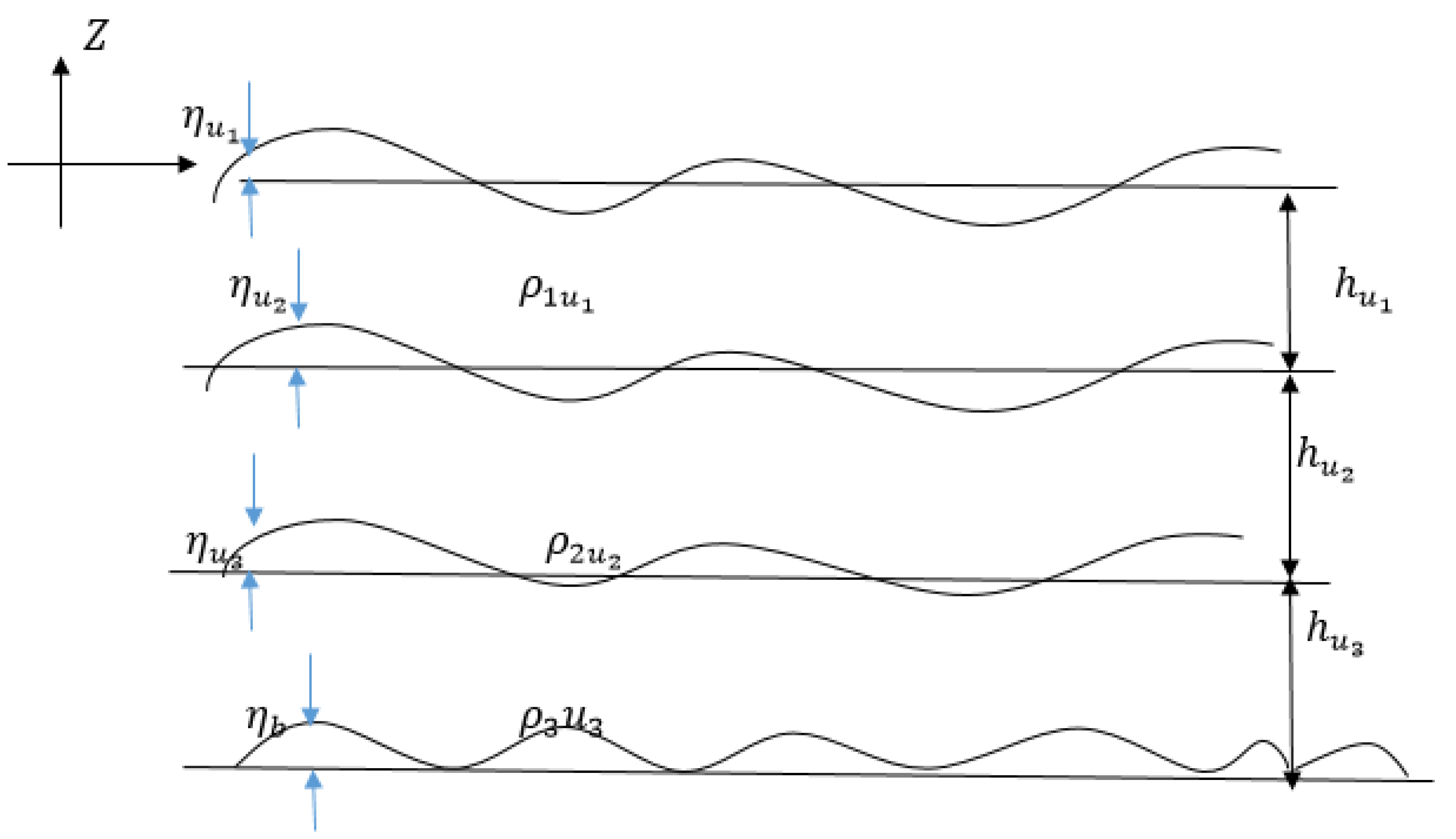
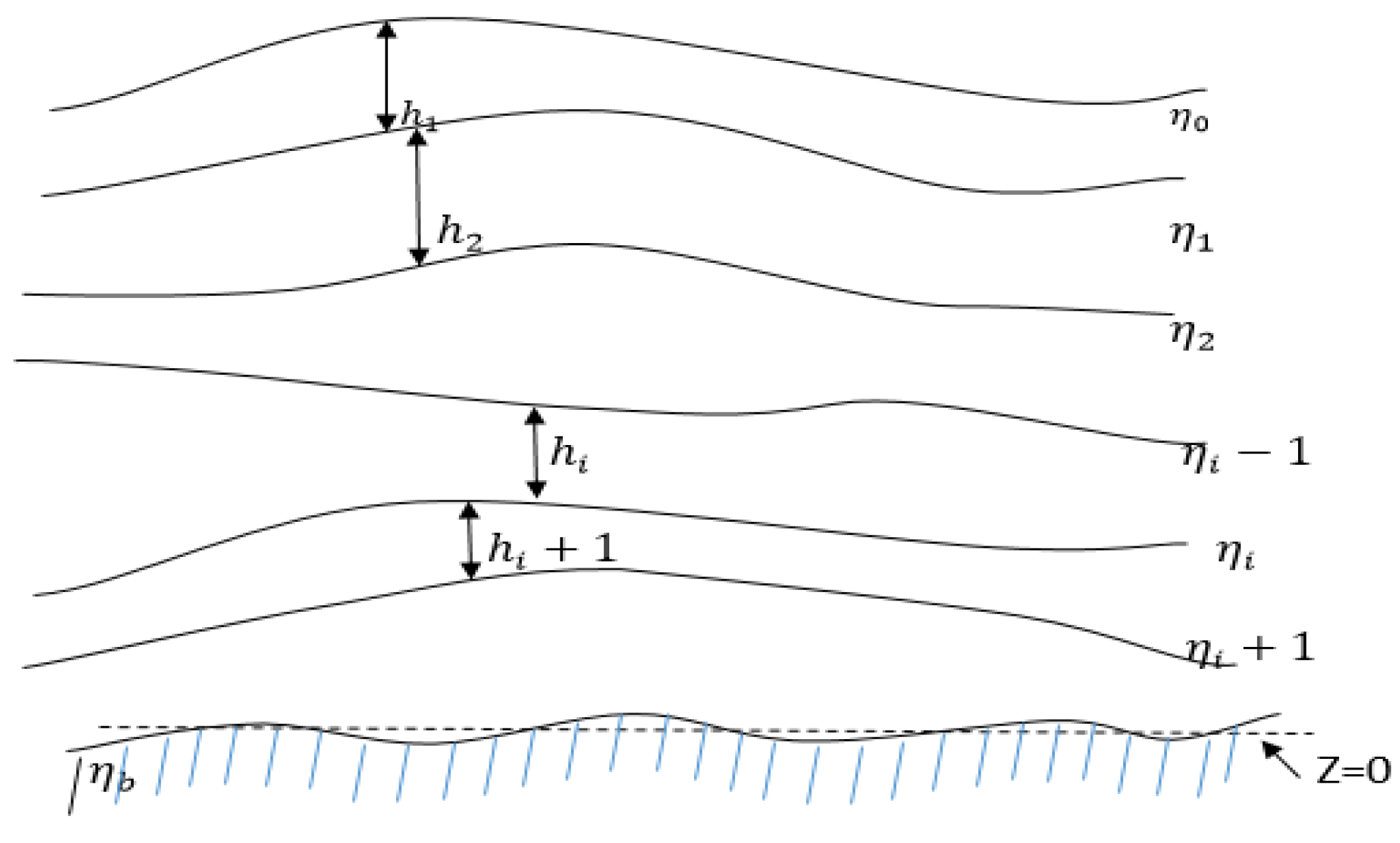
Figure 3. A symmetry of continuous deep water stratification.

Figure 3. A symmetry of continuous deep water stratification.

The substantial derivative of stratified deep property under modified gravity and coriolis effect, $f\left(x,y,z,t\right)inaflowfieldwithvelocityvector$

$U={\left(u,v,w\right)}^T$ is given by

$${\displaystyle \frac{Df}{Dt}}\equiv {\displaystyle \frac{\partial f}{\partial t}}+u{\displaystyle \frac{\partial f}{\partial x}}+v{\displaystyle \frac{\partial f}{\partial y}}+w{\displaystyle \frac{\partial f}{\partial z}}$$

(1)

$$={\displaystyle \frac{\partial f}{\partial t}}+U.\nabla f$$

(2)

$$CurlF=\nabla \times F=\left({\displaystyle \frac{\partial }{\partial x}},{\displaystyle \frac{\partial }{\partial y}},{\displaystyle \frac{\partial }{\partial z}}\right)\times \left(F_1\left(x,y,z\right),F_2\left(x,y,z\right),F_3\left(x,y,z\right)\right)$$

The operator$\nabla$ is a differential operator defined as

$$\nabla \equiv \left({\displaystyle \frac{\partial }{\partial x}},{\displaystyle \frac{\partial }{\partial y}},{\displaystyle \frac{\partial }{\partial z}}\right)$$

(3)

so that $\nabla f={\left(f_x,f_y,f_z\right)}^T$; such that any arbitrary fluid property can be expressed as

$$f\left(x,y,z,t\right)=f\left(x\left(t\right),y\left(t\right),z\left(t\right),t\right)$$

(4)

Differentiating equation (1) with respect to t using chain rule:

$${\displaystyle \frac{df}{dt}}={\displaystyle \frac{\partial f}{\partial x}}{\displaystyle \frac{dx}{dt}}+{\displaystyle \frac{\partial f}{\partial y}}{\displaystyle \frac{dy}{dt}}+{\displaystyle \frac{\partial f}{\partial z}}{\displaystyle \frac{dz}{dt}}+{\displaystyle \frac{\partial f}{\partial t}}{\displaystyle \frac{dt}{dt}}$$

(5)

$$={\displaystyle \frac{\partial f}{\partial t}}+u{\displaystyle \frac{\partial f}{\partial x}}+v{\displaystyle \frac{\partial f}{\partial y}}+w{\displaystyle \frac{\partial f}{\partial z}}$$

(6)

Thus, in the circumstance of velocity components the material derivative is the Lagrangian acceleration which in most cases is the same meaning with Eulerian acceleration. For the x-component of velocity, the substantial derivative from equation (1), we have

$${\displaystyle \frac{Du}{Dt}}={\displaystyle \frac{\partial \left(u\right)}{\partial t}}+u{\displaystyle \frac{\partial \left(u\right)}{\partial x}}+v{\displaystyle \frac{\partial \left(u\right)}{\partial y}}+w{\displaystyle \frac{\partial \left(u\right)}{\partial z}}$$

(7)

${\displaystyle \frac{Du}{Dt}}$ is the total acceleration;

${\displaystyle \frac{\partial u}{\partial t}}$ is the local acceleration;

$u{\displaystyle \frac{\partial \left(u\right)}{\partial x}}+v{\displaystyle \frac{\partial \left(u\right)}{\partial y}}+w{\displaystyle \frac{\partial \left(u\right)}{\partial z}}$ is the convective or advective terms.

This represents the x-direction (Lagrangian, or total) acceleration, $a_x$, of a fluid parcel expressed in Eulerian reference frame. Then in Lagrangian frame the spartial changes in velocity is

$$U.\nabla u={\displaystyle \frac{\partial \left(u\right)}{\partial t}}+u{\displaystyle \frac{\partial \left(u\right)}{\partial x}}+v{\displaystyle \frac{\partial \left(u\right)}{\partial y}}+w{\displaystyle \frac{\partial \left(u\right)}{\partial z}}$$

(8)

Figure 4. cross sectional area pressure of stratified deep water under modified gravity and coriolis effect.

Figure 4. cross sectional area pressure of stratified deep water under modified gravity and coriolis effect.

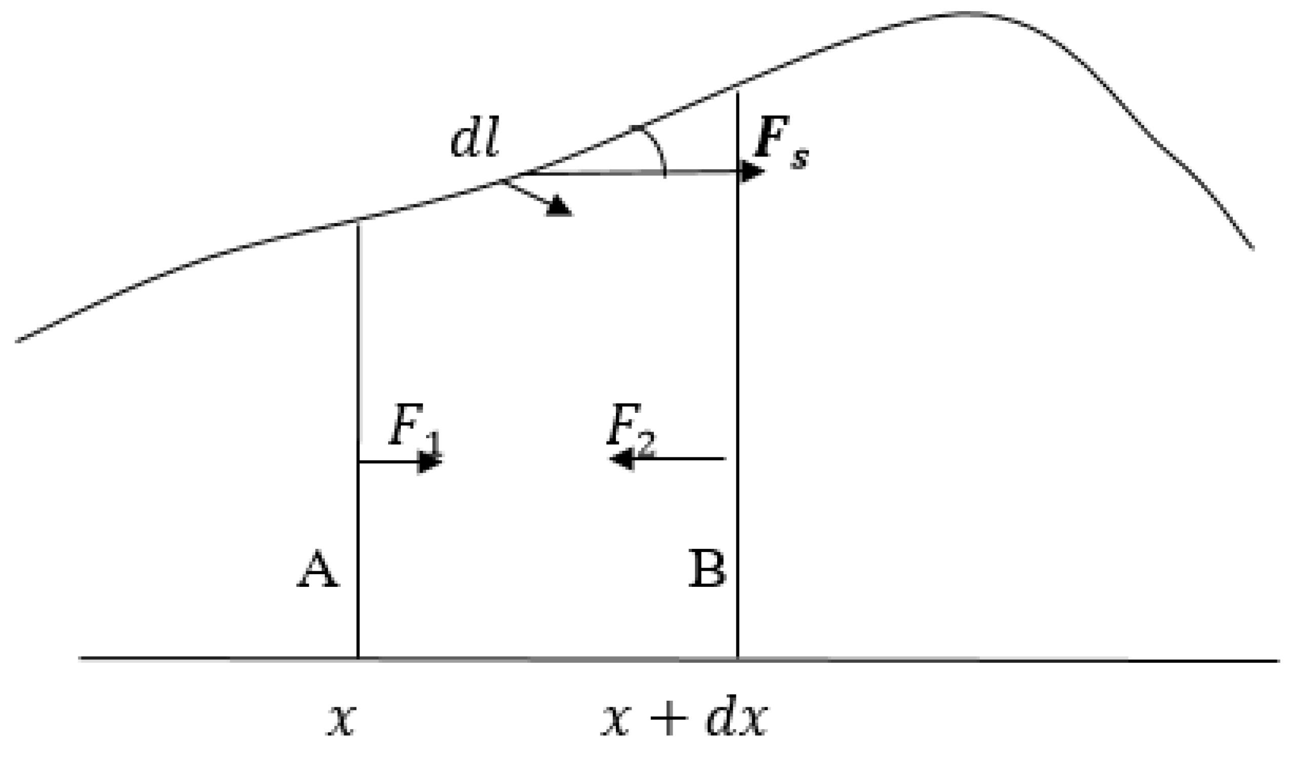
Since the surface area is inclined, the product of pressure and its cross sectional area sustain a non-zero component ${\mathit{p}}_0\mathit{d}\mathit{l}\mathit{s}\mathit{i}\mathit{n}\propto$ stand in the $\mathit{x}$-direction positively, $\left(\propto \right),$ is the interface angle. And, $\mathit{d}\mathit{l}={\displaystyle \frac{\mathit{d}\mathit{x}}{c\mathit{o}\mathit{s}\propto }}$, is influence on the force in x-direction, which is ${\mathit{F}}_{\mathit{s}}={\mathit{p}}_0{\displaystyle \frac{\partial \mathit{h}}{\partial \mathit{x}}}\mathit{d}\mathit{x}$ (but$\mathit{t}\mathit{a}\mathit{n}\propto {\displaystyle \frac{\partial \mathit{h}}{\partial \mathit{x}}}$). From this our net force on the volume, per unit length in$\mathit{y}$, is expressed as:

$$\mathit{F}={\mathit{p}}_0{\displaystyle \frac{\partial \mathit{h}}{\partial \mathit{x}}}\mathit{d}\mathit{x}+{\int }_0^{\mathit{h}}\mathit{p}\left(\mathit{x},\mathit{z}\right)\mathit{d}\mathit{z}-{\int }_0^{\mathit{h}}\mathit{p}\left(\mathit{x}+\mathit{d}\mathit{x},\mathit{z}\right)\mathit{d}\mathit{z}$$

(9)

But, from (9),we have

$$\begin{gathered} {\int }_0^{\mathit{h}}\mathit{p}\mathit{d}\mathit{z}={\int }_0^{\mathit{h}}{\mathit{p}}_0\mathit{d}\mathit{z}+\mathit{\rho }\mathit{g}{\int }_0^{\mathit{h}}\begin{array}{c}\left(\mathit{h}-\mathit{z}\right)dz\end{array} \\ ={\mathit{\rho }}_0\mathit{h}+{\displaystyle \frac{1}{2}}\mathit{\rho }\mathit{g}{\mathit{h}}^2 \end{gathered}$$

(10)

$$\begin{gathered} {\int }_0^{\mathit{h}}\mathit{p}\left(\mathit{x},\mathit{z}\right)\mathit{d}\mathit{z}-{\int }_0^{h}p.\left(x+dx,z\right)dz=p_{0}h\left(x+dx\right)+{\displaystyle \frac{1}{2}}.\rho g{h}^2\left(x\right)-{\displaystyle \frac{1}{2}}\rho g{h}^2.\left(x+dx\right) \\ =-p_0{\displaystyle \frac{\partial h}{\partial x}}dx-\rho gh{\displaystyle \frac{\partial h}{\partial x}}dx \end{gathered}$$

(11)

Therefore for stratified deepwater the acceleration of the volume is given by

$$m{\displaystyle \frac{du}{dt}}=F=-\rho gh{\displaystyle \frac{\partial h}{\partial x}}dx$$

(12)

Now, using our expression$m=\rho hdx$, the preceding equation gives us (cancelling the factors$phdx$)

$${\displaystyle \frac{du}{dt}}=-g{\displaystyle \frac{\partial h}{\partial x}}dx$$

(13)

Our derivative ${\displaystyle \frac{d}{dt}}$ is the substantial derivative that tells us how the velocity of the deep water under modified gravity and coriolis effect changes volume as it travels around and get stratified. This has to be converted into form that tells how the velocity $u$ changes in a stratified coordinate.

$${\displaystyle \frac{du}{dt}}={\displaystyle \frac{\partial u}{\partial t}}+{\displaystyle \frac{dx}{dt}}{\displaystyle \frac{\partial u}{\partial x}}={\displaystyle \frac{\partial u}{\partial t}}+u{\displaystyle \frac{\partial u}{\partial x}}$$

(14)

And thus to write our equation of motion in final form

$${\displaystyle \frac{\partial u}{\partial t}}+u{\displaystyle \frac{\partial u}{\partial x}}=-g{\displaystyle \frac{\partial h}{\partial x}}$$

(15)

Like equation (14), the equation (15) connects the local acceleration in two expressions:

• The pressure slope expression and
• The momentum advection.

Two predictive equations with two unknown velocity and height expressed as $\mathrm{u}(\mathrm{x},\mathrm{t})$and $\mathrm{h}(\mathrm{x},\mathrm{t})$ are obtained from the two equations (14) and (15) which further gives in principle all we need to know to determine how stratified is the deep water and its progress within given initial boundary conditions. The equations are nonlinear and have complex properties in general.

4. Effect of Rotation

There is possibility of extending those equations in two dimensions$(x,y$) with vector velocity $U=(u,v)$ and in order to include rotation therefore we shall add coriolis effect on the equation of momentum, equation (15). Our set of equations will now in vector form become:

$${\displaystyle \frac{\partial u}{\partial t}}+u{\displaystyle \frac{\partial u}{\partial x}}+v{\displaystyle \frac{\partial u}{\partial y}}+fv=-g{\displaystyle \frac{\partial h}{\partial x}}$$

(16)

$${\displaystyle \frac{\partial v}{\partial t}}+u{\displaystyle \frac{\partial v}{\partial x}}+v{\displaystyle \frac{\partial v}{\partial y}}+fu=-g{\displaystyle \frac{\partial h}{\partial y}}$$

(17)

$${\displaystyle \frac{\partial h}{\partial t}}+u{\displaystyle \frac{\partial h}{\partial x}}+v{\displaystyle \frac{\partial h}{\partial y}}=-h\left({\displaystyle \frac{\partial u}{\partial x}}+{\displaystyle \frac{\partial v}{\partial y}}\right)$$

(18)

where $fuandfvaccountfortherotation$ due to coriolis effect.

Now for the modified gravity we employ the concept Topman et al (2024):

$$g{\mathrm{ˈ}}_n=g{\displaystyle \frac{\left({\rho }_{n+1}-{\rho }_n\right)}{{\rho }_n}}$$

(19)

Now for generality we can suppress “n” on $g_n^{\prime }$ to give $g^{\prime }$and express

$$g\mathrm{ˈ}=g{\displaystyle \frac{\left({\rho }_{i+1}-{\rho }_i\right)}{{\rho }_i}}$$

(20)

Where $i=\mathrm{0,1},2,\dots$

5. Model Equation

FOR THE THREE LAYERS MODEL OF A SYSTEM OF NINE PARTIAL DIFFERENTIAL EQUATIONS:

By incorporating the effect of rotation and modified gravity in equations (16), (17) and (18) we obtain our model equations, which are nine set of first order partial differential equations.

$${\displaystyle \frac{\partial \left(h_1{u}_1\right)}{\partial t}}+{\displaystyle \frac{\partial (h_1{u}_1^2+\frac{g{\frac{{\rho }_0-{\rho }_1}{{\rho }_1}h}_1^2}{2}}{\partial x}}=-g{\displaystyle \frac{{\rho }_1-{\rho }_0}{{\rho }_0}}{h}_1{\displaystyle \frac{\partial h_2}{\partial x}}-g{\displaystyle \frac{{\rho }_1-{\rho }_0}{{\rho }_0}}{h}_1{\displaystyle \frac{\partial \left(\xi \right)}{\partial x}}+f{u}_1$$

(21)

$${\displaystyle \frac{\partial \left(h_1{v}_1\right)}{\partial t}}=-g{\displaystyle \frac{{\rho }_1-{\rho }_0}{{\rho }_0}}{h}_1{\displaystyle \frac{\partial \left(\xi \right)}{\partial x}}-f{u}_1$$

(22)

$${\displaystyle \frac{\partial h_1}{\partial t}}+{\displaystyle \frac{\partial \left(h_1{u}_1\right)}{\partial x}}=0$$

(23)

$${\displaystyle \frac{\partial \left(h_2{u}_2\right)}{\partial t}}+{\displaystyle \frac{\partial \left(h_2{u}_2^2+\frac{g\frac{{\rho }_2-{\rho }_1}{{\rho }_1}{h}_2^2}{2}+g\frac{{\rho }_2-{\rho }_1}{{\rho }_1}{h}_2{h}_1\right)}{\partial x}}=-{g{\displaystyle \frac{{\rho }_1-{\rho }_2}{{\rho }_2}}h}_1{\displaystyle \frac{\partial h_2}{\partial x}}-g{\displaystyle \frac{{\rho }_1-{\rho }_2}{{\rho }_2}}{h}_2{\displaystyle \frac{\partial \left(\xi \right)}{\partial x}}+f{u}_2$$

(24)

$${\displaystyle \frac{\partial \left(h_2{v}_2\right)}{\partial t}}=-{g{\displaystyle \frac{{\rho }_2-{\rho }_1}{{\rho }_1}}h}_1{\displaystyle \frac{\partial h_2}{\partial y}}-g{\displaystyle \frac{{\rho }_2-{\rho }_1}{{\rho }_1}}{h}_2{\displaystyle \frac{\partial \left(\xi \right)}{\partial y}}-f{u}_2$$

(25)

$${\displaystyle \frac{\partial h_2}{\partial t}}+{\displaystyle \frac{\partial \left(h_2{u}_2\right)}{\partial x}}=0$$

(26)

$${\displaystyle \frac{\partial \left(h_3{u}_3\right)}{\partial t}}+{\displaystyle \frac{\partial \left(h_3{u}_3^2+\frac{g\frac{{\rho }_3-{\rho }_2}{{\rho }_2}{h}_2^2}{2}+g\frac{{\rho }_3-{\rho }_2}{{\rho }_2}{h}_3{h}_2\right)}{\partial x}}=-{g{\displaystyle \frac{{\rho }_3-{\rho }_2}{{\rho }_2}}h}_1{\displaystyle \frac{\partial h_3}{\partial x}}-g{\displaystyle \frac{{\rho }_3-{\rho }_2}{{\rho }_2}}{h}_3{\displaystyle \frac{\partial \left(\xi \right)}{\partial x}}+f{u}_3$$

(27)

$${\displaystyle \frac{\partial \left(h_3{v}_3\right)}{\partial t}}=-{g{\displaystyle \frac{{\rho }_3-{\rho }_2}{{\rho }_2}}h}_1{\displaystyle \frac{\partial h_2}{\partial y}}-g{\displaystyle \frac{{\rho }_3-{\rho }_2}{{\rho }_2}}{h}_2{\displaystyle \frac{\partial \left(\xi \right)}{\partial y}}-f{u}_3$$

(28)

$${\displaystyle \frac{\partial h_3}{\partial t}}+{\displaystyle \frac{\partial \left(h_3{u}_3\right)}{\partial x}}=0$$

(29)

Equation (21), (22), (23), (24), (25), (26), (27), (28) and (29) are the model equations, Topman et al (2024).

Let us impose necessary boundary condition on our model equations:

With initial condition and boundary condition

$$\left.\begin{array}{c}{u}_1\left(x,0\right)=u_0,u_x\left(0,y,t\right)=0,u_x\left(l,t\right)=0\\ \\ u_2\left(x,0\right)=u_0,u_2\left(x,t\right)=0,u_x\left(x,t\right)=0\\ u_{\left(2\right)x}\left(0,t\right)=0,u_{2\left(x\right)}\left(l,t\right)=0\\ \end{array}\right\}$$

(30)

$$h\left(x,0\right)=m{e}^{-s\left(x^2\right)}-\xi \left(x\right),h_x\left(u,t\right),$$

Where

$\xi \left(x,y\right)=\beta sin\left(\alpha x\right)0\le \alpha \le 90$, and the values of $\beta and\alpha$ which are the measure of stability and measure of strength of the system depends on the size of the stratified layer at thermocline regime.

$$h\left(x,t=0\right)=m{e}^{-s\left(x^2\right)}-\xi \left(x\right)$$

Let us consider this equation so we can expand our model into series

$${\displaystyle \frac{\partial h}{\partial t}}+{\displaystyle \frac{\partial \left(h_{11}{u}_{11}\right)}{\partial x}}+{\displaystyle \frac{\partial \left(h_{21}{u}_{21}\right)}{\partial x}}+{\displaystyle \frac{\partial \left(h_{31}{u}_{31}\right)}{\partial x}}=0{\displaystyle \frac{\partial h}{\partial t}}+{\displaystyle \frac{\partial (h_{11}{u}_{11}+h_{21}{u}_{21}+h_{31}{u}_{31})}{\partial x}}=0$$

(31)

That is,

$${\displaystyle \frac{d{h}_{11}}{dt}}+h_{11}{\displaystyle \frac{\partial \left(u_{11}\right)}{\partial x}}=0$$

(32)

$${\displaystyle \frac{d{h}_{21}}{dt}}+h_{21}{\displaystyle \frac{\partial \left(u_{21}\right)}{\partial x}}=0$$

(33)

$${\displaystyle \frac{d{h}_{31}}{dt}}+h_{31}{\displaystyle \frac{\partial \left(u_{31}\right)}{\partial x}}=0$$

(34)

Therefore,

$${\displaystyle \frac{d{h}_{11}}{dt}}=-h_{11}{\displaystyle \frac{\partial \left(u_{11}\right)}{\partial x}}$$

(35)

$${\displaystyle \frac{d{h}_{21}}{dt}}=-h_{21}{\displaystyle \frac{\partial \left(u_{21}\right)}{\partial x}}$$

(36)

$${\displaystyle \frac{d{h}_{31}}{dt}}=-h_{31}{\displaystyle \frac{\partial \left(u_{31}\right)}{\partial x}}$$

(37)

Note that if, $f=\left(x,y,t\right)\Rightarrow f=(x,t)$, since the variation of velocity in y- direction is very small and then neglected.

$${\displaystyle \frac{df}{dt}}={\displaystyle \frac{\partial f}{\partial t}}.{\displaystyle \frac{dt}{dt}}+{\displaystyle \frac{\partial f}{\partial x}}.{\displaystyle \frac{dx}{dt}}+{\displaystyle \frac{\partial f}{\partial y}}.{\displaystyle \raisebox{1ex}{$dy$}\!\left/ \!\raisebox{-1ex}{$dt$}\right.}$$

(38)

Now, we can rewrite the model equation as,

$${\displaystyle \frac{\partial \left(h_{11}{u}_{11}\right)}{\partial t}}+{\displaystyle \frac{\partial \left(h_{11}{u}_{11}^2+g(\frac{{\rho }_1-{\rho }_0}{{\rho }_0}\right)\raisebox{1ex}{$h_{11}^2$}\!\left/ \!\raisebox{-1ex}{$2$}\right.}{\partial x}}=-g{\displaystyle \frac{{\rho }_1-{\rho }_0}{{\rho }_0}}{\displaystyle \frac{\partial \xi }{\partial x}}+f{u}_{11}$$

(39)

$$u_{11}{\displaystyle \frac{\partial h_{11}}{\partial t}}+h_{11}{\displaystyle \frac{\partial u_{11}}{\partial t}}+u_{11}^2{\displaystyle \frac{\partial h_{11}}{\partial x}}+2h_{11}{u}_{11}{\displaystyle \frac{\partial u_{11}}{\partial x}}+g{{\displaystyle \frac{{\rho }_1-{\rho }_0}{{\rho }_0}}h}_{11}{\displaystyle \frac{\partial h_{11}}{\partial x}}-g{\displaystyle \frac{{\rho }_1-{\rho }_0}{{\rho }_0}}{\displaystyle \frac{\partial \xi }{\partial x}}+f{u}_{11}$$

(40)

This is further simplified as:

$$u_{11}\left({\displaystyle \frac{\partial h_{11}}{\partial t}}+u_{11}{\displaystyle \frac{\partial h_{11}}{\partial x}}\right)+h_{11}\left({\displaystyle \frac{\partial u_{11}}{\partial t}}+2u_{11}{\displaystyle \frac{\partial u_{11}}{\partial x}}\right)+g{\displaystyle \frac{{(\rho }_1-{\rho }_0)}{{\rho }_0}}{h}_{11}{\displaystyle \frac{\partial h_{11}}{\partial x}}=-g{\displaystyle \frac{{(\rho }_0-{\rho }_1)}{{\rho }_1}}{\displaystyle \frac{\partial \xi }{\partial x}}+f{u}_{11}$$

(41)

From equation (41), recall the continuity equation for each of the stratification.

From the first stratification level,

$${\displaystyle \frac{\partial }{\partial t}}\left(h_{11}\right)+{\displaystyle \frac{\partial }{\partial x}}\left(h_{11}{u}_{11}\right)=0$$

(42)

$$\Rightarrow {\displaystyle \frac{\partial }{\partial t}}\left(h_{11}\right)+h_{11}{\displaystyle \frac{\partial }{\partial x}}\left(u_{11}\right)+u_{11}{\displaystyle \frac{\partial \left(h_{11}\right)}{\partial x}}=0$$

(43)

$${\displaystyle \frac{\partial }{\partial t}}\left(h_{11}\right)+u_{11}{\displaystyle \frac{\partial \left(h_{11}\right)}{\partial x}}=-h_{11}{\displaystyle \frac{\partial }{\partial x}}\left(u_{11}\right)$$

(44)

Substituting equation (44) into (41), we get

$$\begin{gathered} -u_{11}{h}_{11}{\displaystyle \frac{\partial u_{11}}{\partial t}}+h_{11}{\displaystyle \frac{\partial }{\partial x}}\left(u_{11}\right)+2u_{11}{h}_{11}{\displaystyle \frac{\partial u_{11}}{\partial x}}+g{h}_{11}{\displaystyle \frac{{\rho }_1-{\rho }_0}{{\rho }_0}}{\displaystyle \frac{\partial h_{11}}{\partial x}}=-g{h}_{11}\left({\displaystyle \frac{{\rho }_1-{\rho }_0}{{\rho }_0}}\right){\displaystyle \frac{\partial \xi }{\partial x}}+f{u}_{11} \\ {h}_{11}\left({\displaystyle \frac{\partial }{\partial t}}{u}_{11}+u_{11}{\displaystyle \frac{\partial }{\partial x}}{u}_{11}\right)+g{h}_{11}\left({\displaystyle \frac{{\rho }_1-{\rho }_0}{{\rho }_0}}\right){\displaystyle \frac{\partial h_{11}}{\partial x}}=-g\left({\displaystyle \frac{{\rho }_1-{\rho }_0}{{\rho }_0}}\right){\displaystyle \frac{\partial \xi }{\partial x}}+f{u}_{11} \end{gathered}$$

(45)

From equation (45),

$$\left({\displaystyle \frac{\partial }{\partial t}}{u}_{11}+u_{11}{\displaystyle \frac{\partial }{\partial x}}{u}_{11}\right)={\displaystyle \frac{d{u}_{11}}{dt}}$$

(46)

Equation (45) becomes;

$$h_{11}{\displaystyle \frac{d{u}_{11}}{dt}}+g{h}_{11}\left({\displaystyle \frac{{\rho }_1-{\rho }_0}{{\rho }_0}}\right){\displaystyle \frac{\partial h_{11}}{\partial x}}=-g\left({\displaystyle \frac{{\rho }_1-{\rho }_0}{{\rho }_0}}\right){\displaystyle \frac{\partial \xi }{\partial x}}+f{u}_{11}$$

(47)

Using (32) in (41), yields;

$$h_{11}{\displaystyle \frac{d{u}_{11}}{dt}}+g{\displaystyle \frac{{(\rho }_1-{\rho }_0)}{{\rho }_0}}{h}_{11}{\displaystyle \frac{\partial h_{11}}{\partial x}}=-g{\displaystyle \frac{{(\rho }_1-{\rho }_0)}{{\rho }_0}}{\displaystyle \frac{\partial \xi }{\partial x}}+f{u}_{11}$$

(48)

Similarly, equation (33) in (41) can be expressed as;

$$u_{21}\left({\displaystyle \frac{\partial h_{21}}{\partial t}}+u_{21}{\displaystyle \frac{\partial h_{21}}{\partial x}}\right)+h_{21}\left({\displaystyle \frac{\partial u_{21}}{\partial t}}+2u_{21}{\displaystyle \frac{\partial u_{21}}{\partial x}}\right)+g{\displaystyle \frac{{(\rho }_2-{\rho }_1)}{{\rho }_1}}{h}_{21}{\displaystyle \frac{\partial h_{21}}{\partial x}}=-g{\displaystyle \frac{{(\rho }_2-{\rho }_1)}{{\rho }_1}}{\displaystyle \frac{\partial \xi }{\partial x}}+f{u}_{21}$$

(49)

Using (4.94) in (4.103), we obtain;

$$h_{21}{\displaystyle \frac{d{u}_{21}}{dt}}+g{\displaystyle \frac{{(\rho }_2-{\rho }_1)}{{\rho }_1}}{h}_{21}{\displaystyle \frac{\partial h_{21}}{\partial x}}=-g{\displaystyle \frac{{(\rho }_2-{\rho }_1)}{{\rho }_1}}{\displaystyle \frac{\partial \xi }{\partial x}}+f{u}_{21}$$

(50)

Again, equation (4.95) in (4.99) can be written as;

$$u_{31}\left({\displaystyle \frac{\partial h_{31}}{\partial t}}+u_{31}{\displaystyle \frac{\partial h_{31}}{\partial x}}\right)+h_{31}\left({\displaystyle \frac{\partial u_{31}}{\partial t}}+2u_{31}{\displaystyle \frac{\partial u_{31}}{\partial x}}\right)+g{\displaystyle \frac{{(\rho }_3-{\rho }_2)}{{\rho }_2}}{h}_{31}{\displaystyle \frac{\partial h_{31}}{\partial x}}=-g{\displaystyle \frac{{(\rho }_3-{\rho }_2)}{{\rho }_2}}{\displaystyle \frac{\partial \xi }{\partial x}}+f{u}_{31}$$

(51)

$$h_{31}{\displaystyle \frac{d{u}_{31}}{dt}}+g{\displaystyle \frac{{(\rho }_2-{\rho }_1)}{{\rho }_1}}{h}_{31}{\displaystyle \frac{\partial h_{31}}{\partial x}}=-g{\displaystyle \frac{{(\rho }_2-{\rho }_1)}{{\rho }_1}}{\displaystyle \frac{\partial \xi }{\partial x}}+f{u}_{31}$$

(52)

Now let $0<f\ll 1,andg=g{\displaystyle \frac{{(\rho }_{i{+}_1}-{\rho }_i)}{{\rho }_i}}=af$

The perturbation method of series solution is a technique used to solve partial differential equations (PDEs) by assuming a solution in the form of an infinite series. In applying this method to solve the PDE of deep water waves, the Coriolis parameter is included on the left-hand side of the equation to account for the effect of rotation on the wave propagation. The inclusion of the Coriolis parameter is important because deep water waves can propagate in the presence of rotation, and this rotation can affect the wave speed and direction. By including the Coriolis parameter on the left-hand side of the equation, the effect of rotation is taken into account, and the solution obtained will be more accurate. Since the coriolis parameter is approximately $7.29\times {10}^{-5}/s$, Gaspard de Coriolis, (1835) which is $\ll 1$, we can equally write the series expansion of the velocities and height in terms of $f$. Thus;

Suppose the solution $(u_{11},u_{21},u_{31},h_{11},h_{21},h_{31})$

$$\left.\begin{array}{c}{u}_{11}\left(x,t\right)=u_{12}\left(x,t\right)+f{u}_{13}\left(x,t\right)+f{u}_{14}^2+\dots \\ u_{21}\left(x,t\right)=u_{22}\left(x,t\right)+f{u}_{23}\left(x,t\right)+f{u}_{24}^2+\dots \\ u_{31}\left(x,t\right)=u_{32}\left(x,t\right)+f{u}_{33}\left(x,t\right)+f{u}_{34}^2+\dots \\ h_{11}\left(x,t\right)=h_{12}\left(x,t\right)+f{h}_{13}\left(x,t\right)+f{u}_{14}^2+\dots \\ h_{21}\left(x,t\right)=h_{22}\left(x,t\right)+f{h}_{23}\left(x,t\right)+f{u}_{24}^2+\dots \\ h_{31}\left(x,t\right)=h_{32}\left(x,t\right)+f{h}_{33}\left(x,t\right)+f{u}_{34}^2+\dots \\ \end{array}\right\}$$

(53)

Substituting equation (53) in (4.93), (33), and (34), we get

$$\left.\begin{array}{c}{\displaystyle \frac{d}{dt}}\left(h_{12}+f{h}_{13}+\dots \right)+\left(h_{12}+f{h}_{13}+\dots \right)\left({\displaystyle \frac{\partial }{\partial x}}\left(u_{12}+f{u}_{13}+\dots \right)+{\displaystyle \frac{\partial }{\partial x}}\left(u_{12}+f{u}_{13}+\dots \right)\right)=0\\ {\displaystyle \frac{d}{dt}}\left(h_{22}+f{h}_{23}+\dots \right)+\left(h_{22}+f{h}_{23}+\dots \right)\left({\displaystyle \frac{\partial }{\partial x}}\left(u_{12}+f{u}_{13}+\dots \right)+{\displaystyle \frac{\partial }{\partial x}}\left(u_{22}+f{u}_{23}+\dots \right)\right)=0\\ {\displaystyle \frac{d}{dt}}\left(h_{32}+f{h}_{33}+\dots \right)+\left(h_{32}+f{h}_{33}+\dots \right)\left({\displaystyle \frac{\partial }{\partial x}}\left(u_{12}+f{u}_{13}+\dots \right)+{\displaystyle \frac{\partial }{\partial x}}\left(u_{32}+f{u}_{33}+\dots \right)\right)=0\end{array}\right\}$$

(54)

Which simplifies to;

$$\left.\begin{array}{c}{\displaystyle \frac{d}{dt}}{h}_{12}+{\displaystyle \frac{d}{dt}}f{h}_{13}+\dots +h_{12}{\displaystyle \frac{\partial }{\partial x}}{u}_{12}+h_{12}{\displaystyle \frac{\partial }{\partial x}}f{u}_{13}+f{h}_{13}{\displaystyle \frac{\partial }{\partial x}}{u}_{12}+f^2{h}_{13}{\displaystyle \frac{\partial }{\partial x}}f{u}_{13}+\dots =0\\ {\displaystyle \frac{d}{dt}}{h}_{22}+{\displaystyle \frac{d}{dt}}f{h}_{23}+\dots +h_{22}{\displaystyle \frac{\partial }{\partial x}}{u}_{22}+h_{22}{\displaystyle \frac{\partial }{\partial x}}f{u}_{23}+f{h}_{23}{\displaystyle \frac{\partial }{\partial x}}{u}_{22}+f^2{h}_{23}{\displaystyle \frac{\partial }{\partial x}}f{u}_{23}+\dots +=0\\ {\displaystyle \frac{d}{dt}}{h}_{32}+{\displaystyle \frac{d}{dt}}f{h}_{33}+\dots +h_{32}{\displaystyle \frac{\partial }{\partial x}}{u}_{32}+h_{32}{\displaystyle \frac{\partial }{\partial x}}f{u}_{33}+f{h}_{33}{\displaystyle \frac{\partial }{\partial x}}{u}_{32}+f^2{h}_{33}{\displaystyle \frac{\partial }{\partial x}}f{u}_{33}+\dots +=0\end{array}\right\}$$

(55)

Substituting equation (53) in (48), we get,

$$\begin{gathered} \left(h_{12}+f{h}_{13}+\dots \right){\displaystyle \frac{d}{dt}}\left(u_{12}+f{u}_{13}+\dots \right)+af\left(h_{12}+f{h}_{13}+\dots \right){\displaystyle \frac{\partial }{\partial x}}(h_{12}+f{h}_{13}+\dots \\ =-af{\displaystyle \frac{\partial \xi }{\partial x}}+f(u_{12}+f{u}_{13}+\dots ) \end{gathered}$$

$$\left.\begin{array}{c}{h}_{12}{\displaystyle \frac{d}{dt}}{u}_{12}+f{h}_{12}{\displaystyle \frac{d}{dt}}{u}_{13}+f{h}_{13}{\displaystyle \frac{d}{dt}}{u}_{12}+f^2{h}_{13}{\displaystyle \frac{d}{dt}}{u}_{13}+\dots +af{h}_{12}{\displaystyle \frac{\partial }{\partial x}}{h}_{12}+a{f}^2{h}_{12}{\displaystyle \frac{\partial }{\partial x}}{h}_{13}+\\ a{f}^2{h}_{13}{\displaystyle \frac{\partial }{\partial x}}{h}_{12}+a{f}^3{h}_{13}{\displaystyle \frac{\partial }{\partial x}}{h}_{13}+\dots +=-af{\displaystyle \frac{\partial \xi }{\partial x}}+f{u}_{12}+f^2{u}_{13}+\dots \end{array}\right\}$$

(56)

Substituting equation (53) in (50), we obtain;

$$\left(h_{12}+f{h}_{13}+\dots \right){\displaystyle \frac{d}{dt}}\left(u_{22}+f{u}_{23}+\dots \right)+af\left(h_{22}+f{h}_{23}+\dots \right){\displaystyle \frac{\partial }{\partial x}}\left(h_{22}+f{h}_{23}+\dots \right)=-af{\displaystyle \frac{\partial \xi }{\partial x}}+f(u_{12}+f{u}_{13}+\dots )$$

(57)

$$\left.\begin{array}{c}{h}_{22}{\displaystyle \frac{d}{dt}}{u}_0+f{h}_{22}{\displaystyle \frac{d}{dt}}{u}_{23}+f{h}_{23}{\displaystyle \frac{d}{dt}}{u}_{22}+f^2{h}_{23}{\displaystyle \frac{d}{dt}}{u}_{23}+\dots +af{h}_{22}{\displaystyle \frac{\partial }{\partial x}}{h}_0+a{f}^2{h}_{22}{\displaystyle \frac{\partial }{\partial x}}{h}_{23}+\\ a{f}^2{h}_{23}{\displaystyle \frac{\partial }{\partial x}}{h}_{22}+a{f}^3{h}_{23}{\displaystyle \frac{\partial }{\partial x}}{h}_{23}+\dots +=-af{\displaystyle \frac{\partial \xi }{\partial x}}+f{u}_{22}+f^2{u}_{23}+\dots \end{array}\right\}$$

(58)

Substituting equation (53) in (52), we obtain;

$$\left.\begin{array}{c}{h}_{32}{\displaystyle \frac{d}{dt}}{u}_{32}+f{h}_{32}{\displaystyle \frac{d}{dt}}{u}_{33}+f{h}_{33}{\displaystyle \frac{d}{dt}}{u}_{32}+f^2{h}_{33}{\displaystyle \frac{d}{dt}}{u}_{33}+\dots +af{h}_{32}{\displaystyle \frac{\partial }{\partial x}}{h}_{32}+a{f}^2{h}_{32}{\displaystyle \frac{\partial }{\partial x}}{h}_{33}+\\ a{f}^2{h}_{33}{\displaystyle \frac{\partial }{\partial x}}{h}_{32}+a{f}^3{h}_{33}{\displaystyle \frac{\partial }{\partial x}}{h}_{33+\dots +}=-af{\displaystyle \frac{\partial \xi }{\partial x}}+f{u}_{32}+f^2{u}_{33}+\dots \end{array}\right\}$$

(59)

Comparing the coefficient of powers of$f$from (56), (58) and (59), we have;

$$\begin{gathered} f^0 \\ {h}_{12}{\displaystyle \frac{d{u}_{12}}{dt}}=0;u_{13}\left(x,0\right)=u_{13} \end{gathered}$$

(60)

$$h_{22}{\displaystyle \frac{d{u}_{22}}{dt}}=0;u_{23}\left(x,0\right)=u_{23}$$

(61)

$$h_{32}{\displaystyle \frac{d{u}_{32}}{dt}}=0;u_{33}\left(x,0\right)=u_{33}$$

(62)

$$\left.\begin{array}{c}{\displaystyle \frac{d{h}_{12}}{dt}}=-h_{12}\left({\displaystyle \frac{\partial u_{13}}{\partial x}}\right);h_{12}\left(x,0\right)=m{e}^{-s\left(x^2\right)}-\xi \left(x,0\right)\\ {\displaystyle \frac{d{h}_{22}}{dt}}=-h_{22}\left({\displaystyle \frac{\partial u_{23}}{\partial x}}\right);h_{22}\left(x,0\right)=m{e}^{-s\left(x^2\right)}-\xi \left(x,0\right)\\ {\displaystyle \frac{d{h}_{32}}{dt}}=-h_{32}\left({\displaystyle \frac{\partial u_{33}}{\partial x}}\right);h_{32}\left(x,0\right)=m{e}^{-s\left(x^2\right)}-\xi \left(x,0\right)\\ \\ \end{array}\right\}$$

(63)

$$\begin{gathered} f^1 \\ \left.\begin{array}{c}{h}_{12}{\displaystyle \frac{d{u}_{13}}{dt}}+h_{13}{\displaystyle \frac{d{u}_{12}}{dt}}+a{h}_{12}{\displaystyle \frac{\partial h_{12}}{\partial x}}=-a{\displaystyle \frac{\partial \xi }{\partial x}}+u_{12};u_{13}\left(x,0\right)=0\\ h_{22}{\displaystyle \frac{d{u}_{23}}{dt}}+h_{23}{\displaystyle \frac{d{u}_{22}}{dt}}+a{h}_{22}{\displaystyle \frac{\partial h_{22}}{\partial x}}=-a{\displaystyle \frac{\partial \xi }{\partial x}}+u_{22};u_{23}\left(x,0\right)=0\\ h_{32}{\displaystyle \frac{d{u}_{33}}{dt}}+h_{33}{\displaystyle \frac{d{u}_{32}}{dt}}+a{h}_{32}{\displaystyle \frac{\partial h_{32}}{\partial x}}=-a{\displaystyle \frac{\partial \xi }{\partial x}}+u_{32};u_{33}\left(x,0\right)=0\end{array}\right\} \end{gathered}$$

(64)

$${\displaystyle \frac{d{h}_{13}}{dt}}+h_{12}{\displaystyle \frac{\partial u_{13}}{\partial x}}+h_{13}{\displaystyle \frac{\partial u_{12}}{\partial x}}=0$$

(65)

$${\displaystyle \frac{d{h}_{23}}{dt}}+h_{22}{\displaystyle \frac{\partial u_{23}}{\partial x}}+h_{23}{\displaystyle \frac{\partial u_{22}}{\partial x}}=0$$

(66)

$${\displaystyle \frac{d{h}_{33}}{dt}}+h_{32}{\displaystyle \frac{\partial u_3}{\partial x}}+h_{33}{\displaystyle \frac{\partial u_{32}}{\partial x}}=0$$

(67)

$$\begin{gathered} f^2 \\ \left.\begin{array}{c}{h}_{13}{\displaystyle \frac{d}{dt}}{u}_{13}+{ah}_{12}{\displaystyle \frac{\partial }{\partial x}}{h}_{13}+a{h}_{13}{\displaystyle \frac{\partial }{\partial x}}{h}_{12}=u_{13};u_{13}\left(x,0\right)=0\\ h_{23}{\displaystyle \frac{d}{dt}}{u}_{23}+{ah}_{22}{\displaystyle \frac{\partial }{\partial x}}{h}_{23}+a{h}_{23}{\displaystyle \frac{\partial }{\partial x}}{h}_{22}=u_{23};u_{23}\left(x,0\right)=0\\ h_{33}{\displaystyle \frac{d}{dt}}{u}_{33}+{ah}_{32}{\displaystyle \frac{\partial }{\partial x}}{h}_{33}+a{h}_{33}{\displaystyle \frac{\partial }{\partial x}}{h}_{32}=u_{33};u_{33}\left(x,0\right)=0\end{array}\right\} \end{gathered}$$

(68)

$$\begin{gathered} f^3 \\ \left.\begin{array}{c}{ah}_{13}{\displaystyle \frac{\partial }{\partial x}}{h}_{13=0}\\ {ah}_{23}{\displaystyle \frac{\partial }{\partial x}}{h}_{23=0}\\ {ah}_{33}{\displaystyle \frac{\partial }{\partial x}}{h}_{33=0}\\ \end{array}\right\} \end{gathered}$$

(69)

Now integrating (60) with respect to t, we have;

$$\begin{gathered} u_{12}\left(x,t\right)=c_{13}=constant \\ {u}_{12}\left(x,0\right)=c_{13}=u_{12} \\ {u}_{12}\left(x,t\right)=u_{12} \end{gathered}$$

(70)

Integrating (61) with respect to $t$, we have;

$$u_{22}\left(x,t\right)=c_{23}=constant{u}_{22}\left(x,0\right)=c_{23}=u_{22}$$

Then

$$u_{22}\left(x,t\right)=u_{22}$$

(71)

By using (70) and (71), equation (62) reduces to

$${\displaystyle \frac{d{h}_{32}}{dt}}=-h_{32}\left(0\right)=0$$

(72)

$${\displaystyle \frac{d{h}_{32}}{dt}}=0$$

(73)

$$h_{32}\left(x,0\right)=d-\xi \left(x,0\right)=m{e}^{-s\left(x^2\right)}-\beta \sin \left(\alpha x\right)$$

(74)

$$=m{e}^{-s{x}^2}-\beta \sin \left(\alpha x\right)$$

(75)

Integrating with respect to t, gives;

$$h_{32}\left(x,t\right)=c_{33}=constant$$

$$h_{32}\left(x,0\right)=c_{33}=m{e}^{-s\left(x^2\right)}-\xi (x,0)$$

(76)

$$h_{32}\left(x,t\right)=m{e}^{-s{x}^2}-\beta \sin \left(\alpha x\right)$$

(77)

Using (70), (71) and (77), equation (64) reduces to

$${\displaystyle \frac{d{u}_{13}}{dt}}={\displaystyle \frac{-h_{13}\frac{d{u}_{12}}{dt}-a{h}_{12}\frac{\partial h_{12}}{\partial x}-a\frac{\partial \xi }{\partial x}+u_{12}}{h_{12}}}=-{\displaystyle \frac{h_{13}}{h_{12}}}{\displaystyle \frac{d{u}_{12}}{dt}}-a{\displaystyle \frac{\partial h_{12}}{\partial x}}-{\displaystyle \frac{a}{h_{12}}}{\displaystyle \frac{\partial \xi }{\partial x}}+{\displaystyle \frac{u_{12}}{h_{12}}}$$

(78)

$${\displaystyle \frac{d{u}_{13}}{dt}}=2amsx{e^{-s}}^{{(x}^2)}+\alpha \alpha \beta cos\alpha x-{\displaystyle \frac{\alpha \alpha \beta cos\alpha x}{m{e}^{-s{x}^2}-\beta \sin \alpha x}}+{\displaystyle \frac{u_{12}}{m{e}^{-s{x}^2}-\beta \sin \alpha x}}$$

(79)

Integrating with respect to $t$, we have

$$u_{13}=\left(2amsx{e^{-s}}^{{(x}^2)}+\alpha \alpha \beta cos\alpha x-{\displaystyle \frac{\alpha \alpha \beta cos\alpha x}{m{e}^{-s{x}^2}-\beta \sin \alpha x}}+{\displaystyle \frac{u_0}{m{e}^{-s{x}^2}-\beta \sin \alpha x}}\right)t+c_{10}$$

(80)

But $u_{13}\left(x,0\right)=0⟹c_{10}=0$

$$u_{13}\left(x,t\right)=\left(2amsx{e^{-s}}^{x^2}+\alpha \alpha \beta cos\alpha x-{\displaystyle \frac{\alpha \alpha \beta cos\alpha x}{m{e}^{-s{x}^2}-\beta \sin \alpha x}}+{\displaystyle \frac{u_0}{m{e}^{-s{x}^2}-\beta \sin \alpha x}}\right)t$$

(81)

Using (70), (71) and (77), equation (64)) reduces to

$${\displaystyle \frac{d{u}_{23}}{dt}}={\displaystyle \frac{-h_{23}\frac{d{u}_{22}}{dt}-a{h}_{22}\frac{\partial h_{22}}{\partial x}-a\frac{\partial \xi }{\partial x}+u_{22}}{h_0}}=-{\displaystyle \frac{h_{23}}{h_0}}{\displaystyle \frac{d{u}_{22}}{dt}}-a{\displaystyle \frac{\partial h_{22}}{\partial x}}-{\displaystyle \frac{a}{h_0}}{\displaystyle \frac{\partial \xi }{\partial x}}+{\displaystyle \frac{u_{22}}{h_{22}}}$$

(82)

$${\displaystyle \frac{d{u}_{23}}{dt}}=2amsx{e^{-s}}^{{(x}^2)}+\alpha \alpha \beta cos\alpha x-{\displaystyle \frac{\alpha \alpha \beta cos\alpha x}{m{e}^{-s{x}^2}-\beta \sin \alpha x}}+{\displaystyle \frac{u_{22}}{m{e}^{-s{x}^2}-\beta \sin \alpha x}}$$

(83)

Integrating with respect to $t,$ we get

$$u_{23}=\left(2amsx{e^{-s}}^{{(x}^2)}+\alpha \alpha \beta cos\alpha x-{\displaystyle \frac{\alpha \alpha \beta cos\alpha x}{m{e}^{-s{x}^2}-\beta \sin \alpha x}}+{\displaystyle \frac{u_{22}}{m{e}^{-s{x}^2}-\beta \sin \alpha x}}\right)t+c_{20}$$

(84)

But $u_{23}\left(x,0\right)=0\Rightarrow c_{20}=0$

$$u_{23}\left(x,t\right)=\left(2amsx{e^{-s}}^{{(x}^2)}+\alpha \alpha \beta cos\alpha x-{\displaystyle \frac{\alpha \alpha \beta cos\alpha x}{m{e}^{-s{x}^2}-\beta \sin \alpha x}}+{\displaystyle \frac{u_{22}}{m{e}^{-s{x}^2}-\beta \sin \alpha x}}\right)t$$

(85)

Using (70), (71) and (77), equation (64) reduces to

$${\displaystyle \frac{d{u}_{33}}{dt}}={\displaystyle \frac{-h_{33}\frac{d{u}_{32}}{dt}-a{h}_{32}\frac{\partial h_{32}}{\partial x}-a\frac{\partial \xi }{\partial x}+u_{32}}{h_0}}=-{\displaystyle \frac{h_{33}}{h_{32}}}{\displaystyle \frac{d{u}_{32}}{dt}}-a{\displaystyle \frac{\partial h_{32}}{\partial x}}-{\displaystyle \frac{a}{h_{32}}}{\displaystyle \frac{\partial \xi }{\partial x}}+{\displaystyle \frac{u_{32}}{h_{32}}}$$

(86)

$${\displaystyle \frac{d{u}_{33}}{dt}}=2amsx{e^{-s}}^{{(x}^2)}+\alpha \alpha \beta cos\alpha x-{\displaystyle \frac{\alpha \alpha \beta cos\alpha x}{m{e}^{-s{x}^2}-\beta \sin \alpha x}}+{\displaystyle \frac{u_{32}}{m{e}^{-s{x}^2}-\beta \sin \alpha x}}$$

(87)

Integrating with respect to $t,$ we get

$$u_{33}=\left(2amsx{e^{-s}}^{{(x}^2)}+\alpha \alpha \beta cos\alpha x-{\displaystyle \frac{\alpha \alpha \beta cos\alpha x}{m{e}^{-s{x}^2}-\beta \sin \alpha x}}+{\displaystyle \frac{u_{32}}{m{e}^{-s{x}^2}-\beta \sin \alpha x}}\right)t+c_{30}$$

(87)

But $u_{33}\left(x,0\right)=0\Rightarrow c_{30}=0$

$$u_{33}\left(x,t\right)=\left(2amsx{e^{-s}}^{{(x}^2)}+\alpha \alpha \beta cos\alpha x-{\displaystyle \frac{\alpha \alpha \beta cos\alpha x}{m{e}^{-s{x}^2}-\beta \sin \alpha x}}+{\displaystyle \frac{u_{32}}{m{e}^{-s{x}^2}-\beta \sin \alpha x}}\right)t$$

(88)

Now using (70), (71), (77), (81) and (85), equation (65) becomes;

$${\displaystyle \frac{d{h}_{13}}{dt}}=-h_{12}\left({\displaystyle \frac{\partial u_1}{\partial x}}\right)-h_{13}\left({\displaystyle \frac{\partial u_{12}}{\partial x}}\right)$$

(89)

That is

$${\displaystyle \frac{d{h}_{13}}{dt}}=-h_{12}\left({\displaystyle \frac{\partial u_{13}}{\partial x}}\right)$$

(90)

This simplifies to;

$${\displaystyle \frac{\partial u_{13}}{\partial x}}=\left(\begin{array}{c}\begin{array}{c}2amsx{e^{-s}}^{x^2}-4am{s}^2{x}^2{e}^{-s{x}^2}+a{\alpha }^2\beta \sin \left(\alpha x\right)-\\ {\displaystyle \frac{m\alpha \beta e^{-s{x}^2}\left(2cos\alpha x-sin\alpha x\right)+a{\alpha }^2{\beta }^2({\sin }^2\alpha x+{\cos }^2\alpha x)}{{\left(m{e}^{-s{x}^2}-\beta sin\alpha x\right)}^2}}+u_{12}{\displaystyle \frac{(2mx{e}^{-s{x}^2}+\alpha \beta cos\alpha x)}{{\left(m{e}^{-s{x}^2}-\beta sin\alpha x\right)}^2}}\end{array}\end{array}\right)t$$

(91)

$${\displaystyle \frac{d{h}_{13}}{dt}}=-\left(m{e}^{-s{x}^2}-\beta sin\alpha x\right)\left(\begin{array}{c}\begin{array}{c}2amsx{e^{-s}}^{x^2}-4am{s}^2{x}^2{e}^{-s{x}^2}+a{\alpha }^2\beta \sin \left(\alpha x\right)-\\ {\displaystyle \frac{m\alpha \beta e^{-s{x}^2}\left(2cos\alpha x-sin\alpha x\right)+a{\alpha }^2{\beta }^2({\sin }^2\alpha x+{\cos }^2\alpha x)}{{\left(m{e}^{-s{x}^2}-\beta sin\alpha x\right)}^2}}+u_{12}{\displaystyle \frac{(2mx{e}^{-s{x}^2}+\alpha \beta cos\alpha x)}{{\left(m{e}^{-s{x}^2}-\beta sin\alpha x\right)}^2}}\end{array}\end{array}\right)t$$

(92)

Integrating with respect to t, we get

$$h_{13}=-\left(m{e}^{-s{x}^2}-\beta sin\alpha x\right)\left(\begin{array}{c}\begin{array}{c}2amsx{e^{-s}}^{x^2}-4am{s}^2{x}^2{e}^{-s{x}^2}+a{\alpha }^2\beta \sin \left(\alpha x\right)-\\ {\displaystyle \frac{m\alpha \beta e^{-s{x}^2}\left(2cos\alpha x-sin\alpha x\right)+a{\alpha }^2{\beta }^2}{{\left(m{e}^{-s{x}^2}-\beta sin\alpha x\right)}^2}}+u_{12}{\displaystyle \frac{(2mx{e}^{-s{x}^2}+\alpha \beta cos\alpha x)}{{\left(m{e}^{-s{x}^2}-\beta sin\alpha x\right)}^2}}\end{array}\end{array}\right){\displaystyle \raisebox{1ex}{$t^2$}\!\left/ \!\raisebox{-1ex}{$2$}\right.}+c_7$$

(93)

Since ${\sin }^2\alpha x+{\cos }^2\alpha x=1$

$$\therefore h_{13}=-\left(m{e}^{-s{x}^2}-\beta sin\alpha x\right)\left(\begin{array}{c}\begin{array}{c}2amsx{e^{-s}}^{x^2}-4am{s}^2{x}^2{e}^{-s{x}^2}+a{\alpha }^2\beta \sin \left(\alpha x\right)-\\ {\displaystyle \frac{m\alpha \beta e^{-s{x}^2}\left(2cos\alpha x-sin\alpha x\right)+a{\alpha }^2{\beta }^2}{{\left(m{e}^{-s{x}^2}-\beta sin\alpha x\right)}^2}}+u_{12}{\displaystyle \frac{(2mx{e}^{-s{x}^2}+\alpha \beta cos\alpha x)}{{\left(m{e}^{-s{x}^2}-\beta sin\alpha x\right)}^2}}\end{array}\end{array}\right){\displaystyle \raisebox{1ex}{$t^2$}\!\left/ \!\raisebox{-1ex}{$2$}\right.}$$

(94)

$$\begin{gathered} h_{13}=-t^{2}g{\displaystyle \frac{{\rho }_1-{\rho }_0}{{\rho }_0}}{m}^{2}sx{e}^{-2s{x}^2}+t^2\beta sin\alpha xg{\displaystyle \frac{{\rho }_1-{\rho }_0}{{\rho }_0}}msx{e^{-s}}^{x^2}+2t^{2}g{\displaystyle \frac{{\rho }_1-{\rho }_0}{{\rho }_0}}{m}^2{s}^2{x}^2{e}^{-2s{x}^2}- \\ 2t^2\beta \sin \left(\alpha x\right)g{\displaystyle \frac{{\rho }_1-{\rho }_0}{{\rho }_0}}m{s}^2{x}^2{e}^{-s{x}^2}-{\displaystyle \frac{1}{2}}{t}^{2}m{e}^{-s{x}^2}g{\displaystyle \frac{{\rho }_1-{\rho }_0}{{\rho }_0}}{\alpha }^2\beta \sin \left(\alpha x\right)+{\displaystyle \frac{1}{2}}{t}^{2}g{\displaystyle \frac{{\rho }_1-{\rho }_0}{{\rho }_0}}{\alpha }^2{\beta }^2{\sin }^2\left(\alpha x\right)+ \\ {\displaystyle \frac{1}{2}}{t}^2{\displaystyle \frac{m^2\alpha \beta e^{-2s{x}^2}\left(2cos\alpha x-sin\alpha x\right)+m{e}^{-s{x}^2}g\frac{{\rho }_1-{\rho }_0}{{\rho }_0}{\alpha }^2{\beta }^2}{{\left(m{e}^{-s{x}^2}-\beta sin\alpha x\right)}^2}}-{\displaystyle \frac{1}{2}}{t}^2{\displaystyle \frac{m\alpha {\beta }^2\sin \left(\alpha x\right)e^{-s{x}^2}\left(2cos\alpha x-sin\alpha x\right)+g\frac{{\rho }_1-{\rho }_0}{{\rho }_0}{\alpha }^2{\beta }^3\sin \left(\alpha x\right)}{{\left(m{e}^{-s{x}^2}-\beta sin\alpha x\right)}^2}}- \\ {\displaystyle \frac{1}{2}}{t}^2{u}_{12}m{e}^{-s{x}^2}{\displaystyle \frac{(2mx{e}^{-s{x}^2}+\alpha \beta cos\alpha x)}{{\left(m{e}^{-s{x}^2}-\beta sin\alpha x\right)}^2}}+{\displaystyle \frac{1}{2}}{t}^2{u}_{12\beta \mathrm{s}\mathrm{i}\mathrm{n}\left(\alpha x\right)}{\displaystyle \frac{(2mx{e}^{-s{x}^2}+\alpha \beta cos\alpha x)}{{\left(m{e}^{-s{x}^2}-\beta sin\alpha x\right)}^2}} \end{gathered}$$

(95)

Equation (95) is the height of the first stratified column under the modified gravity and coriolis effect.

From equation (66);

$${\displaystyle \frac{d{h}_{23}}{dt}}+h_{22}{\displaystyle \frac{\partial u_{23}}{\partial x}}+h_{23}{\displaystyle \frac{\partial u_{22}}{\partial x}}=0$$

$${\displaystyle \frac{d{h}_{23}}{dt}}=-h_{22}\left({\displaystyle \frac{\partial u_{23}}{\partial x}}\right)$$

So

$${\displaystyle \frac{\partial u_{23}}{\partial x}}=\left(\begin{array}{c}\begin{array}{c}2ams{e^{-s}}^{x^2}-4am{s}^2{e}^{-s{x}^2}+a{\alpha }^2\beta \sin \left(\alpha x\right)-\\ {\displaystyle \frac{m\alpha \beta e^{-s{x}^2}\left(2cos\alpha x-sin\alpha x\right)+a{\alpha }^2{\beta }^2({\sin }^2\alpha x+{\cos }^2\alpha x)}{{\left(m{e}^{-s{x}^2}-\beta sin\alpha x\right)}^2}}+u_{22}{\displaystyle \frac{(2ms{e}^{-s{x}^2}+\alpha \beta cos\alpha x)}{{\left(m{e}^{-s{x}^2}-\beta sin\alpha x\right)}^2}}\end{array}\end{array}\right)t$$

(96)

$${\displaystyle \frac{d{h}_{23}}{dt}}=-\left(m{e}^{-s{x}^2}-\beta sin\alpha x\right)\left(\begin{array}{c}\begin{array}{c}2amsx{e^{-s}}^{x^2}-4am{s}^2{x}^2{e}^{-s{x}^2}+a{\alpha }^2\beta \sin \left(\alpha x\right)-\\ {\displaystyle \frac{m\alpha \beta e^{-s{x}^2}\left(2cos\alpha x-sin\alpha x\right)+a{\alpha }^2{\beta }^2({\sin }^2\alpha x+{\cos }^2\alpha x)}{{\left(m{e}^{-s{x}^2}-\beta sin\alpha x\right)}^2}}+u_{22}{\displaystyle \frac{(2mx{e}^{-s{x}^2}+\alpha \beta cos\alpha x)}{{\left(m{e}^{-s{x}^2}-\beta sin\alpha x\right)}^2}}\end{array}\end{array}\right)t$$

(97)

Integrating with respect to t, we get

$$h_{23}=-\left(m{e}^{-s{x}^2}-\beta sin\alpha x\right)\left(\begin{array}{c}\begin{array}{c}2amsx{e^{-s}}^{x^2}-4am{s}^2{x}^2{e}^{-s{x}^2}+a{\alpha }^2\beta \sin \left(\alpha x\right)-\\ {\displaystyle \frac{m\alpha \beta e^{-s{x}^2}\left(2cos\alpha x-sin\alpha x\right)+a{\alpha }^2{\beta }^2}{{\left(m{e}^{-s{x}^2}-\beta sin\alpha x\right)}^2}}+u_{22}{\displaystyle \frac{(2mx{e}^{-s{x}^2}+\alpha \beta cos\alpha x)}{{\left(m{e}^{-s{x}^2}-\beta sin\alpha x\right)}^2}}\end{array}\end{array}\right){\displaystyle \raisebox{1ex}{$t^2$}\!\left/ \!\raisebox{-1ex}{$2$}\right.}+c_8$$

(98)

Since ${\sin }^2\alpha x+{\cos }^2\alpha x=1$

$$\therefore h_{23}=-\left(m{e}^{-s{x}^2}-\beta sin\alpha x\right)\left(\begin{array}{c}\begin{array}{c}2ams{e^{-s}}^{x^2}-4am{s}^2{e}^{-s{x}^2}+a{\alpha }^2\beta \sin \left(\alpha x\right)-\\ {\displaystyle \frac{m\alpha \beta e^{-s{x}^2}\left(2cos\alpha x-sin\alpha x\right)+a{\alpha }^2{\beta }^2}{{\left(m{e}^{-s{x}^2}-\beta sin\alpha x\right)}^2}}+u_{22}{\displaystyle \frac{(2m{e}^{-s{x}^2}+\alpha \beta cos\alpha x)}{{\left(m{e}^{-s{x}^2}-\beta sin\alpha x\right)}^2}}\end{array}\end{array}\right){\displaystyle \raisebox{1ex}{$t^2$}\!\left/ \!\raisebox{-1ex}{$2$}\right.}$$

(99)

$$\begin{gathered} h_{23}(x,t)=-t^{2}g{\displaystyle \frac{{\rho }_2-{\rho }_1}{{\rho }_1}}{m}^{2}sx{e}^{-2s{x}^2}+t^2\beta sin\alpha xg{\displaystyle \frac{{\rho }_2-{\rho }_1}{{\rho }_1}}msx{e^{-s}}^{x^2}+2t^{2}g{\displaystyle \frac{{\rho }_2-{\rho }_1}{{\rho }_1}}{m}^2{s}^2{x}^2{e}^{-2s{x}^2} \\ -2t^2\beta \sin \left(\alpha x\right)g{\displaystyle \frac{{\rho }_2-{\rho }_1}{{\rho }_1}}m{s}^2{x}^2{e}^{-s{x}^2}-{\displaystyle \frac{1}{2}}{t}^{2}m{e}^{-s{x}^2}g{\displaystyle \frac{{\rho }_2-{\rho }_1}{{\rho }_1}}{\alpha }^2\beta \sin \left(\alpha x\right)+{\displaystyle \frac{1}{2}}{t}^{2}g{\displaystyle \frac{{\rho }_2-{\rho }_1}{{\rho }_1}}{\alpha }^2{\beta }^2{\sin }^2\left(\alpha x\right)+ \\ {\displaystyle \frac{1}{2}}{t}^2{\displaystyle \frac{m^2\alpha \beta e^{-2s{x}^2}\left(2cos\alpha x-sin\alpha x\right)+m{e}^{-s{x}^2}g\frac{{\rho }_2-{\rho }_1}{{\rho }_1}{\alpha }^2{\beta }^2}{{\left(m{e}^{-s{x}^2}-\beta sin\alpha x\right)}^2}}-{\displaystyle \frac{1}{2}}{t}^2{\displaystyle \frac{m\alpha {\beta }^2\sin \left(\alpha x\right)e^{-s{x}^2}\left(2cos\alpha x-sin\alpha x\right)+g\frac{{\rho }_2-{\rho }_1}{{\rho }_1}{\alpha }^2{\beta }^3\sin \left(\alpha x\right)}{{\left(m{e}^{-s{x}^2}-\beta sin\alpha x\right)}^2}}- \\ {\displaystyle \frac{1}{2}}{t}^2{u}_{22}m{e}^{-s{x}^2}{\displaystyle \frac{(2mx{e}^{-s{x}^2}+\alpha \beta cos\alpha x)}{{\left(m{e}^{-s{x}^2}-\beta sin\alpha x\right)}^2}}+{\displaystyle \frac{1}{2}}{t}^2{u}_{22\beta \mathrm{s}\mathrm{i}\mathrm{n}\left(\alpha x\right)}{\displaystyle \frac{(2mx{e}^{-s{x}^2}+\alpha \beta cos\alpha x)}{{\left(m{e}^{-s{x}^2}-\beta sin\alpha x\right)}^2}} \end{gathered}$$

(100)

Now using (70), (71), (77), (81) and (85), equation (67) becomes;

$${\displaystyle \frac{d{h}_{33}}{dt}}=-h_{32}\left({\displaystyle \frac{\partial u_{33}}{\partial x}}\right)-h_{33}\left({\displaystyle \frac{\partial u_{32}}{\partial x}}\right)$$

That is

$${\displaystyle \frac{d{h}_{33}}{dt}}=-h_{32}\left({\displaystyle \frac{\partial u_{33}}{\partial x}}\right)$$

This becomes,

$${\displaystyle \frac{\partial u_{33}}{\partial x}}=\left(\begin{array}{c}\begin{array}{c}2ams{e^{-s}}^{x^2}-4am{s}^2{e}^{-s{x}^2}+a{\alpha }^2\beta \sin \left(\alpha x\right)-\\ {\displaystyle \frac{m\alpha \beta e^{-s{x}^2}\left(2cos\alpha x-sin\alpha x\right)+a{\alpha }^2{\beta }^2({\sin }^2\alpha x+{\cos }^2\alpha x)}{{\left(m{e}^{-s{x}^2}-\beta sin\alpha x\right)}^2}}+u_{32}{\displaystyle \frac{(2mx{e}^{-s{x}^2}+\alpha \beta cos\alpha x)}{{\left(m{e}^{-s{x}^2}-\beta sin\alpha x\right)}^2}}\end{array}\end{array}\right)t$$

(101)

$${\displaystyle \frac{d{h}_{33}}{dt}}=-\left(m{e}^{-s{x}^2}-\beta sin\alpha x\right)\left(\begin{array}{c}(z\begin{array}{c}2ams{e^{-s}}^{x^2}-4am{s}^2{e}^{-s{x}^2}+a{\alpha }^2\beta \sin \left(\alpha x\right)-\\ {\displaystyle \frac{m\alpha \beta e^{-s{x}^2}\left(2cos\alpha x-sin\alpha x\right)+a{\alpha }^2{\beta }^2({\sin }^2\alpha x+{\cos }^2\alpha x)}{{\left(m{e}^{-s{x}^2}-\beta sin\alpha x\right)}^2}}+u_{32}{\displaystyle \frac{(2ms{e}^{-s{x}^2}+\alpha \beta cos\alpha x)}{{\left(m{e}^{-s{x}^2}-\beta sin\alpha x\right)}^2}}\end{array}\end{array}\right)t$$

(102)

Integrating with respect to t, we get

$$h_{33}=-\left(m{e}^{-s{x}^2}-\beta sin\alpha x\right)\left(\begin{array}{c}\begin{array}{c}2amsx{e^{-s}}^{x^2}-4am{s}^2{x}^2{e}^{-s{x}^2}+a{\alpha }^2\beta \sin \left(\alpha x\right)-\\ {\displaystyle \frac{m\alpha \beta e^{-s{x}^2}\left(2cos\alpha x-sin\alpha x\right)+a{\alpha }^2{\beta }^2}{{\left(m{e}^{-s{x}^2}-\beta sin\alpha x\right)}^2}}+u_{32}{\displaystyle \frac{(2mx{e}^{-s{x}^2}+\alpha \beta cos\alpha x)}{{\left(m{e}^{-s{x}^2}-\beta sin\alpha x\right)}^2}}\end{array}\end{array}\right){\displaystyle \raisebox{1ex}{$t^2$}\!\left/ \!\raisebox{-1ex}{$2$}\right.}+c_9$$

(103)

Since ${\sin }^2\alpha x+{\cos }^2\alpha x=0$

$$\therefore h_{33}=-\left(m{e}^{-s{x}^2}-\beta sin\alpha x\right)\left(\begin{array}{c}\begin{array}{c}2amsx{e^{-s}}^{x^2}-4am{s}^2{x}^2{e}^{-s{x}^2}+a{\alpha }^2\beta \sin \left(\alpha x\right)-\\ {\displaystyle \frac{m\alpha \beta e^{-s{x}^2}\left(2cos\alpha x-sin\alpha x\right)+a{\alpha }^2{\beta }^2}{{\left(m{e}^{-s{x}^2}-\beta sin\alpha x\right)}^2}}+u_{32}{\displaystyle \frac{(2mx{e}^{-s{x}^2}+\alpha \beta cos\alpha x)}{{\left(m{e}^{-s{x}^2}-\beta sin\alpha x\right)}^2}}\end{array}\end{array}\right){\displaystyle \raisebox{1ex}{$t^2$}\!\left/ \!\raisebox{-1ex}{$2$}\right.}$$

(104)

$$\begin{gathered} h_{33}(x,t)=-t^{2}g{\displaystyle \frac{{\rho }_3-{\rho }_2}{{\rho }_2}}{m}^{2}sx{e}^{-2s{x}^2}+t^2\beta sin\alpha xg{\displaystyle \frac{{\rho }_3-{\rho }_2}{{\rho }_2}}msx{e^{-s}}^{x^2}+2t^{2}g{\displaystyle \frac{{\rho }_3-{\rho }_2}{{\rho }_2}}{m}^2{s}^2{x}^2{e}^{-2s{x}^2}- \\ 2t^2\beta \sin \left(\alpha x\right)g{\displaystyle \frac{{\rho }_3-{\rho }_2}{{\rho }_2}}m{s}^2{x}^2{e}^{-s{x}^2}-{\displaystyle \frac{1}{2}}{t}^{2}m{e}^{-s{x}^2}g{\displaystyle \frac{{\rho }_3-{\rho }_2}{{\rho }_2}}{\alpha }^2\beta \sin \left(\alpha x\right)+{\displaystyle \frac{1}{2}}{t}^{2}g{\displaystyle \frac{{\rho }_3-{\rho }_2}{{\rho }_2}}{\alpha }^2{\beta }^2{\sin }^2\left(\alpha x\right)+ \\ {\displaystyle \frac{1}{2}}{t}^2{\displaystyle \frac{m^2\alpha \beta e^{-2s{x}^2}\left(2cos\alpha x-sin\alpha x\right)+m{e}^{-s{x}^2}g\frac{{\rho }_3-{\rho }_2}{{\rho }_2}{\alpha }^2{\beta }^2}{{\left(m{e}^{-s{x}^2}-\beta sin\alpha x\right)}^2}}-{\displaystyle \frac{1}{2}}{t}^2{\displaystyle \frac{m\alpha {\beta }^2\sin \left(\alpha x\right)e^{-s{x}^2}\left(2cos\alpha x-sin\alpha x\right)+g\frac{{\rho }_3-{\rho }_2}{{\rho }_2}{\alpha }^2{\beta }^3\sin \left(\alpha x\right)}{{\left(m{e}^{-s{x}^2}-\beta sin\alpha x\right)}^2}}- \\ {\displaystyle \frac{1}{2}}{t}^2{u}_{32}m{e}^{-s{x}^2}{\displaystyle \frac{(2mx{e}^{-s{x}^2}+\alpha \beta cos\alpha x)}{{\left(m{e}^{-s{x}^2}-\beta sin\alpha x\right)}^2}}+{\displaystyle \frac{1}{2}}{t}^2{u}_{32\beta \mathrm{s}\mathrm{i}\mathrm{n}\left(\alpha x\right)}{\displaystyle \frac{(2mx{e}^{-s{x}^2}+\alpha \beta cos\alpha x)}{{\left(m{e}^{-s{x}^2}-\beta sin\alpha x\right)}^2}} \end{gathered}$$

(105)

So the velocity in the first layer becomes:

$$u_{13}\left(x,t\right)=u_{12}\left(x,t\right)+f{u}_{13}(x,t)+f^2{u}_{14}\left(x,t\right)+\dots$$

$$u_{13}\left(x,t\right)=u_{12}+f\left(2ams{e^{-s}}^{x^2}+\alpha \alpha \beta cos\alpha x-{\displaystyle \frac{\alpha \alpha \beta cos\alpha x}{m{e}^{-s{x}^2}-\beta \sin \alpha x}}+{\displaystyle \frac{u_0}{m{e}^{-s{x}^2}-\beta \sin \alpha x}}\right)t$$

(106)

The term $f^2{u}_{14}\left(x,t\right)$ varnishes since coriolis parameter $f$ is extremely small. And

$$u_{23}\left(x,t\right)=u_{22}\left(x,t\right)+f{u}_{23}+f^2{u}_{24}\left(x,t\right)+\dots$$

$$u_{23}\left(x,t\right)=u_{22}+\left(\begin{array}{c}f(2ams{e^{-s}}^{x^2}+\alpha \alpha \beta cos\alpha x-{\displaystyle \frac{\alpha \alpha \beta cos\alpha x}{m{e}^{-s{x}^2}-\beta \sin \alpha x}}+{\displaystyle \frac{u_{22}}{m{e}^{-s{x}^2}-\beta \sin \alpha x}})\\ \end{array}\right)t$$

(107)

This simplifies to:

$$u_{23}\left(x,t\right)=u_{22}+\left(\begin{array}{c}f(2g{\displaystyle \frac{{\rho }_2-{\rho }_1}{{\rho }_1}}ms{e^{-s}}^{x^2}+g{\displaystyle \frac{{\rho }_2-{\rho }_1}{{\rho }_1}}\alpha \beta cos\alpha x-{\displaystyle \frac{g\frac{{\rho }_2-{\rho }_1}{{\rho }_1}\alpha \beta cos\alpha x}{m{e}^{-s{x}^2}-\beta \sin \alpha x}}+{\displaystyle \frac{u_{22}}{m{e}^{-s{x}^2}-\beta \sin \alpha x}})\\ \end{array}\right)t$$

(108)

Equation (108) is the velocity at the second layer.

And

$$u_{33}\left(x,t\right)=u_{32}\left(x,t\right)+f{u}_{33}+f^2{u}_{34}\left(x,t\right)+\dots$$

$$u_{33}\left(x,t\right)=u_{32}+\left(\begin{array}{c}f(2g{\displaystyle \frac{{\rho }_2-{\rho }_1}{{\rho }_1}}ms{e^{-s}}^{x^2}+g{\displaystyle \frac{{\rho }_2-{\rho }_1}{{\rho }_1}}\alpha \beta cos\alpha x-{\displaystyle \frac{g\frac{{\rho }_2-{\rho }_1}{{\rho }_1}\alpha \beta cos\alpha x}{m{e}^{-s{x}^2}-\beta \sin \alpha x}}+{\displaystyle \frac{u_{32}}{m{e}^{-s{x}^2}-\beta \sin \alpha x}})\end{array}\right)t$$

(109)

Equation (109) is the velocity in the third layer for the stratified deep water under modified gravity and coriolis effect.

6. The ${\mathit{N}}^{\mathit{t}\mathit{h}}$ Stratified Column

We consider continuously stratified deep water up to nth layer and derive a general equation for the series expansion.

$n_b$ is the nth stratified layer at bottom.

$$h_{10}{\displaystyle \frac{d{u}_{11}}{dt}}+h_{11}{\displaystyle \frac{d{u}_{10}}{dt}}+a{h}_{10}\left({\displaystyle \frac{\partial h_{10}}{\partial x}}\right)=-a{\displaystyle \frac{\partial \xi }{\partial x}}+u_{10}$$

(110)

$$h_{20}{\displaystyle \frac{d{u}_{21}}{dt}}+h_{21}{\displaystyle \frac{d{u}_{20}}{dt}}+a{h}_{20}\left({\displaystyle \frac{\partial h_{20}}{\partial x}}\right)=-a{\displaystyle \frac{\partial \xi }{\partial x}}+u_{20}$$

(111)

$$h_{30}{\displaystyle \frac{d{u}_{31}}{dt}}+h_{31}{\displaystyle \frac{d{u}_{30}}{dt}}+a{h}_{30}\left({\displaystyle \frac{\partial h_{30}}{\partial x}}\right)=-a{\displaystyle \frac{\partial \xi }{\partial x}}+u_{30}$$

(112)

$${\displaystyle \frac{d{h}_{11}}{dt}}=-h_{11}\left({\displaystyle \frac{\partial u_{10}}{\partial x}}\right)-h_{10}\left({\displaystyle \frac{\partial u_{11}}{\partial x}}\right)$$

(113)

$${\displaystyle \frac{d{h}_{21}}{dt}}=-h_{21}\left({\displaystyle \frac{\partial u_{20}}{\partial x}}\right)-h_{20}\left({\displaystyle \frac{\partial u_{21}}{\partial x}}\right)$$

(114)

$${\displaystyle \frac{d{h}_{31}}{dt}}=-h_{31}\left({\displaystyle \frac{\partial u_{30}}{\partial x}}\right)-h_{30}\left({\displaystyle \frac{\partial u_{31}}{\partial x}}\right)$$

(115)

Equation (110-115) are the equations of heights for stratified columns as we have established.

Similarly, for the infinite layers of stratified deep water, that is for nth dimensional space we have

$$h_{n0}{\displaystyle \frac{d{u}_{n1}}{dt}}+h_{n1}{\displaystyle \frac{d{u}_{n0}}{dt}}+a{h}_{n0}\left(\begin{array}{c}{\displaystyle \frac{\partial h_{10}}{\partial x}}+{\displaystyle \frac{\partial h_{20}}{\partial x}}+{\displaystyle \frac{\partial h_{30}}{\partial x}}+\dots +\partial u_{n0}\end{array}\right)+n{h}_{(n-1)0}a{\displaystyle \frac{\partial h_{n0}}{\partial x}}=-a{h}_{n0}{\displaystyle \frac{\partial \xi }{\partial x}}+u_{n0}$$

(116)

And

$${\displaystyle \frac{d{h}_{n+1}}{dt}}=-h_{n1}\left({\displaystyle \frac{\partial u_{n0}}{\partial x}}\right)-h_{n0}{\displaystyle \frac{\partial u_{n1}}{\partial x}}$$

(117)

Where n=1,2, …

Equation (116) and (117) are the general equation of conservation or momentum equation and the general continuity equation for nth layers of stratified deep water respectively under the influence of modified gravity and Coriolis effect.

7. Result

Figure 4. The impact of velocity with measure of stability at various values $\beta =0.05,0.1,0.3and0.5$.

Figure 4. The impact of velocity with measure of stability at various values $\beta =0.05,0.1,0.3and0.5$.

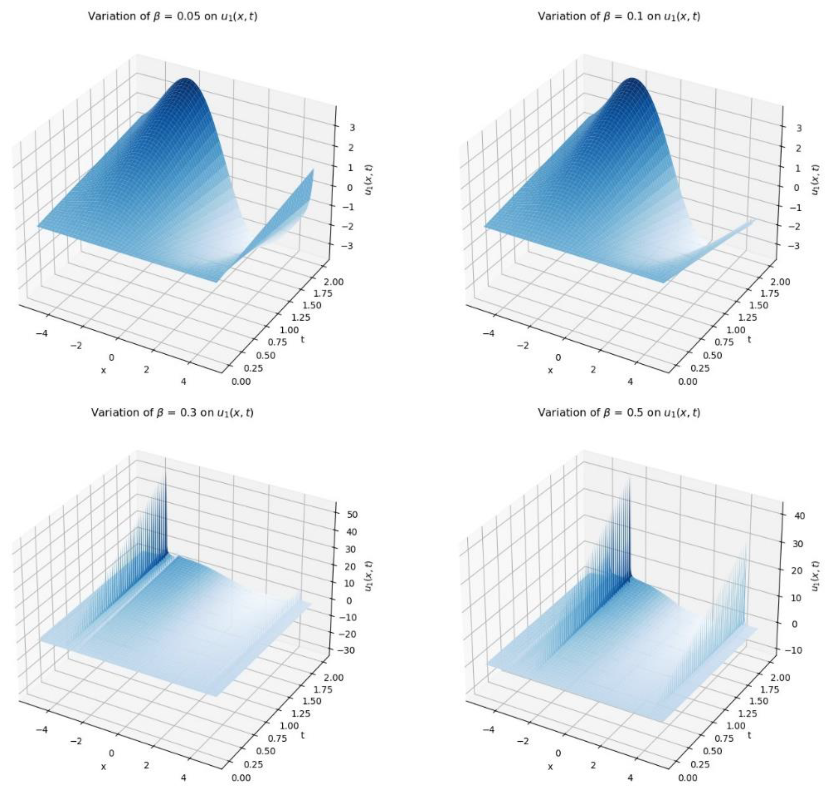
Figure 5. The effect of velocities on the three stratified layers of deep water under modified gravity and Coriolis effect.

Figure 5. The effect of velocities on the three stratified layers of deep water under modified gravity and Coriolis effect.

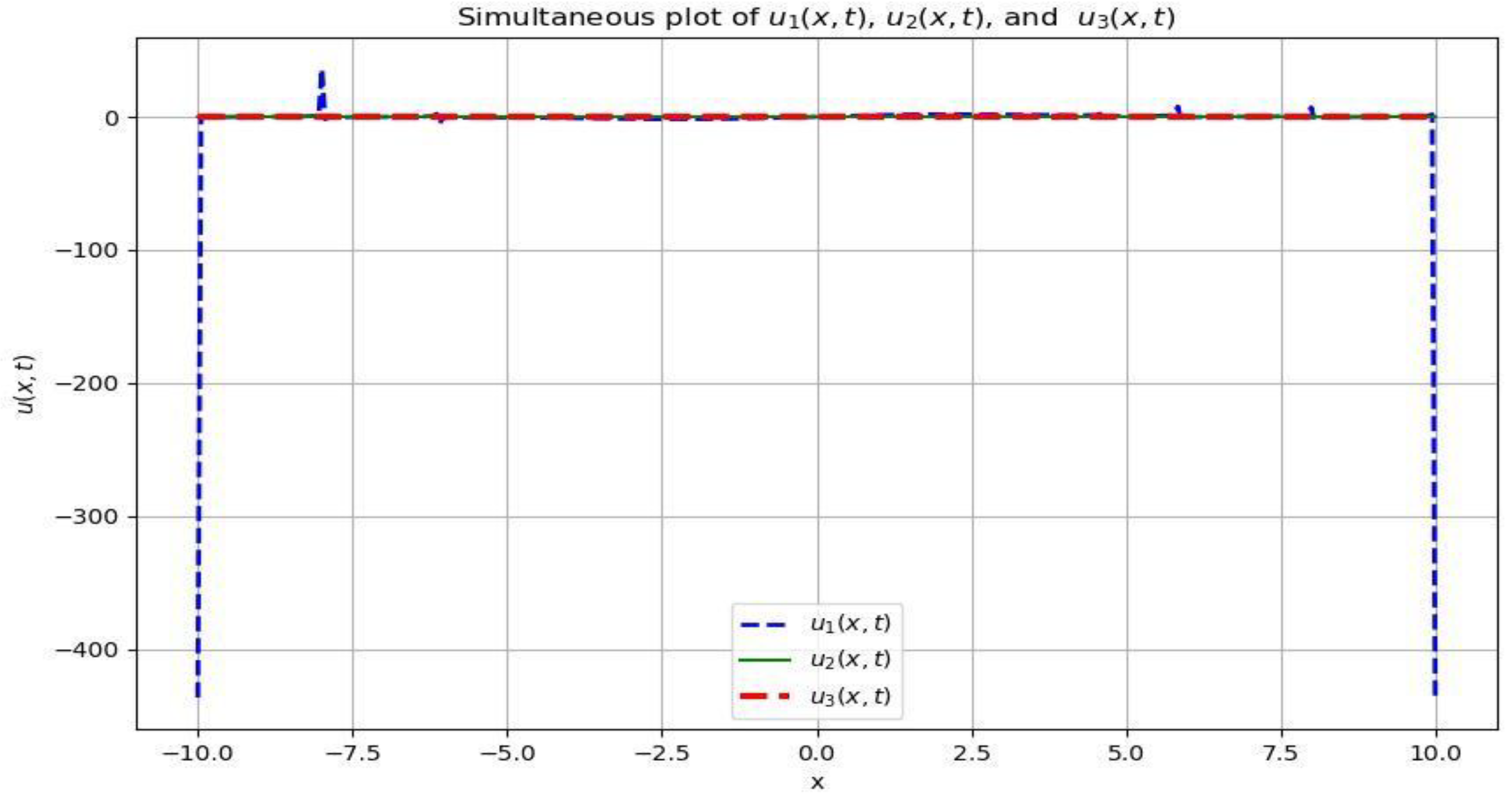
Here the velocity at the first stratified layer is faster and the spec or bubble shows its interaction with the air molecules, the velocities at second and third layers are slower due to density variation leading to gravity modification which causes the stratification. Between $-7.5to5.0$ the velocities $u_1,u_{2}and{u}_3$ are at phase due to the interactions between the internal waves in the three strata.

Figure 6. The impact of modified gravity on the velocity of the first layer.

Figure 6. The impact of modified gravity on the velocity of the first layer.

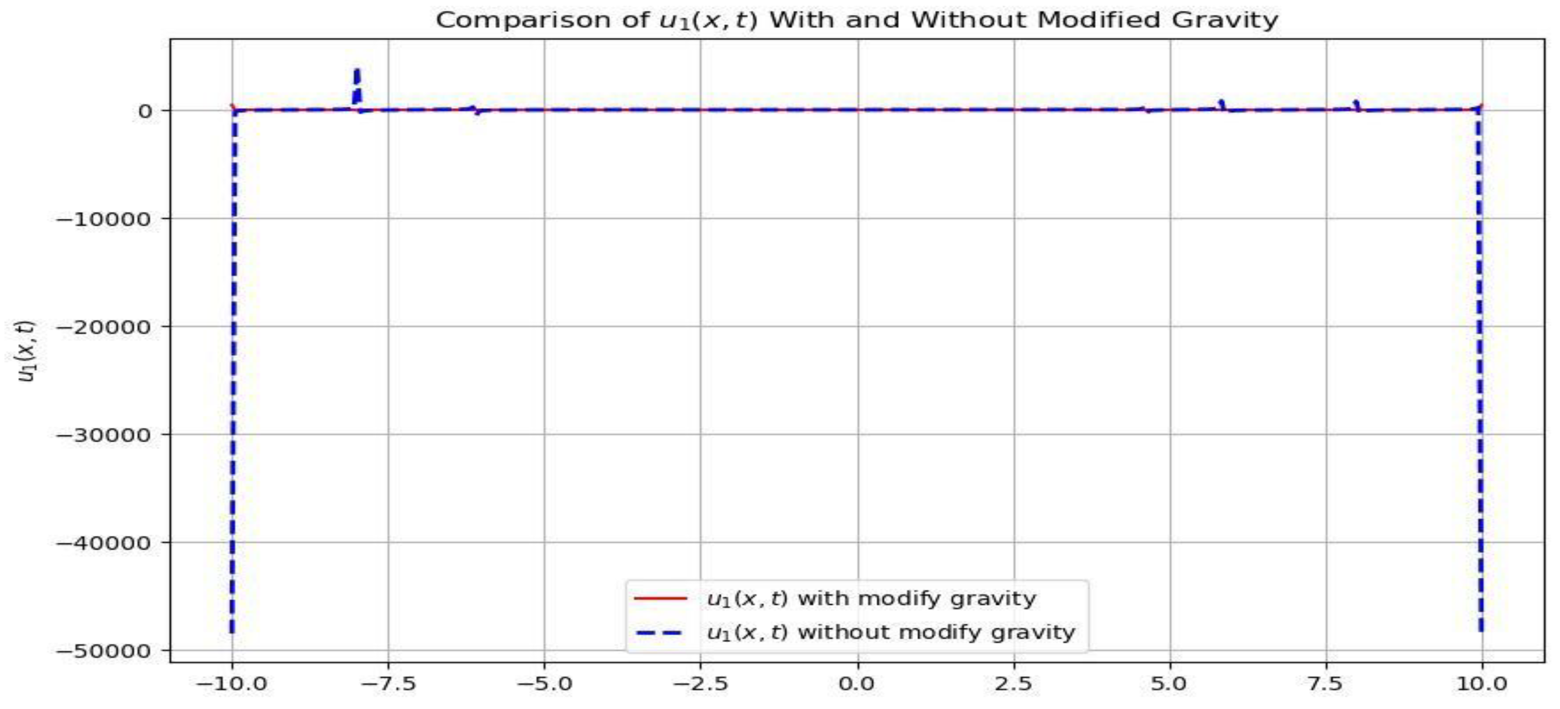
At normal gravity of $9.8m/s^2$ the velocity in first column is faster due to salinity and temperature of the surface water but slows down when gravity is modified leading to stratification.

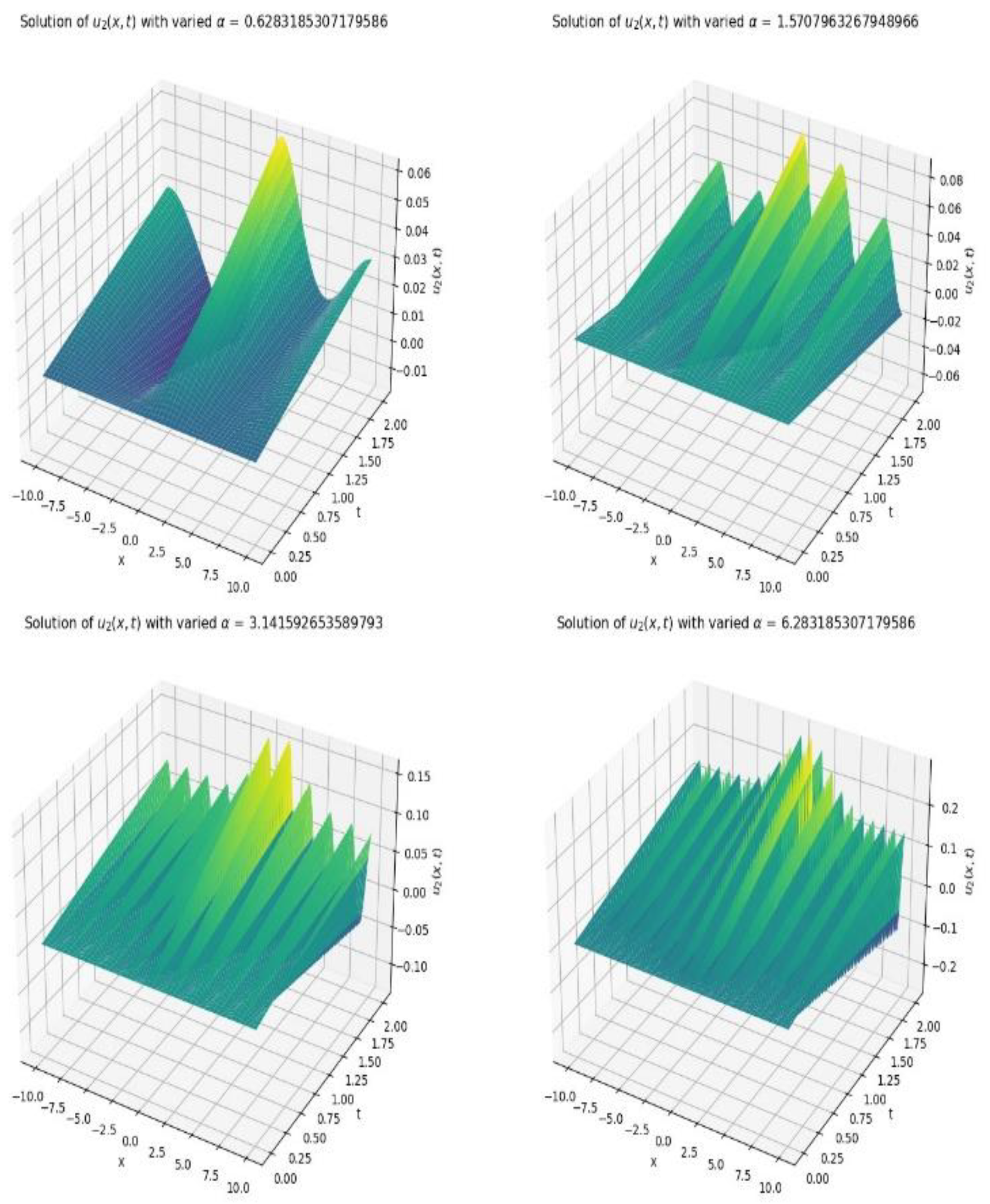
Figure 7. The impact of modified gravity on the velocity of the second stratified layer.

Figure 7. The impact of modified gravity on the velocity of the second stratified layer.

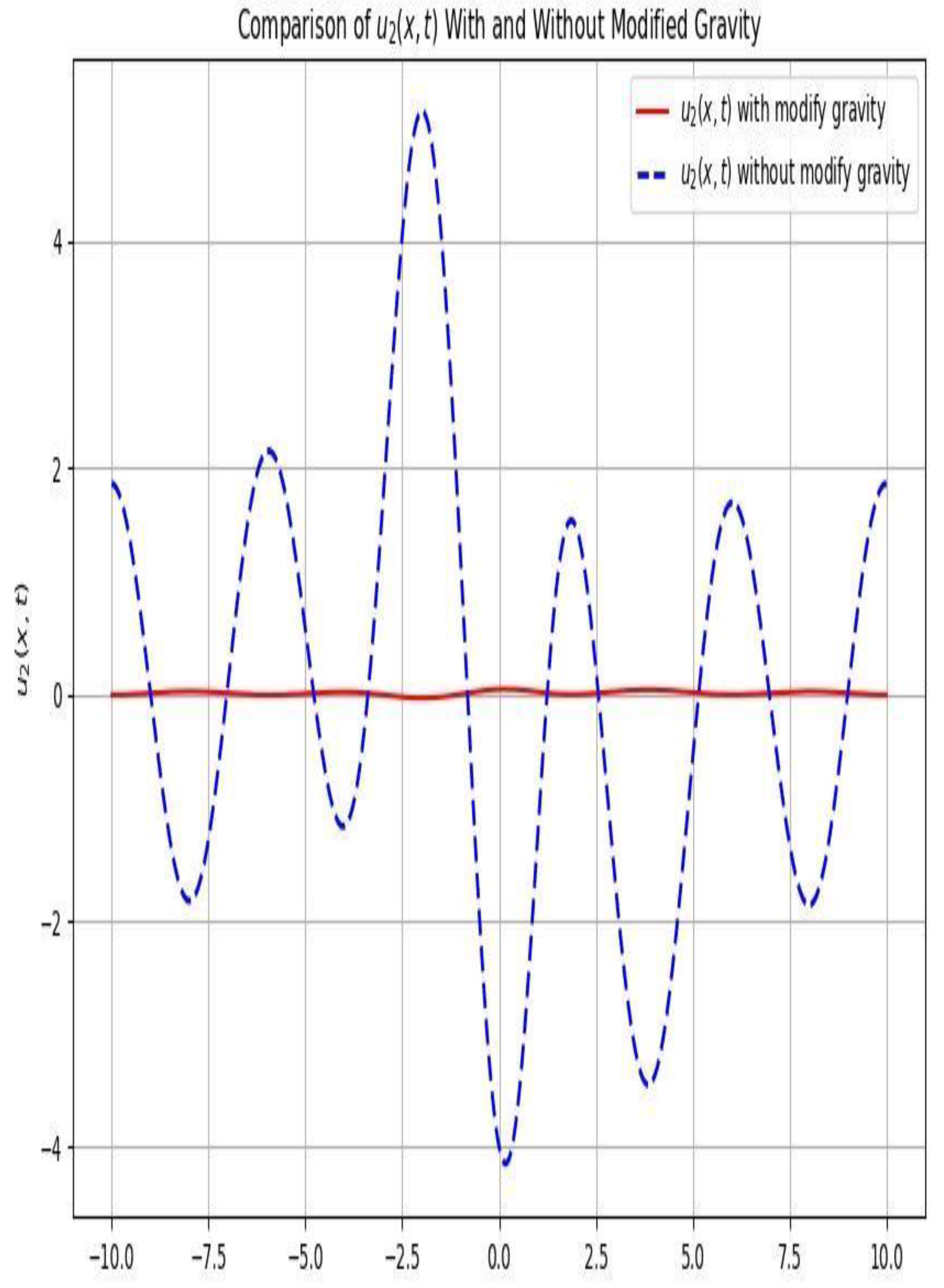
Without the presence of modified gravity the motion is sinusoidal or oscillatory and has its highest amplitude at (0,0) which is at the equilibrium position, but when modified gravity is introduced the motion become nearly uniform and the deep water is stratified at second layer

Figure 8. The impact of modified gravity on third layer of stratified deep water.

Figure 8. The impact of modified gravity on third layer of stratified deep water.

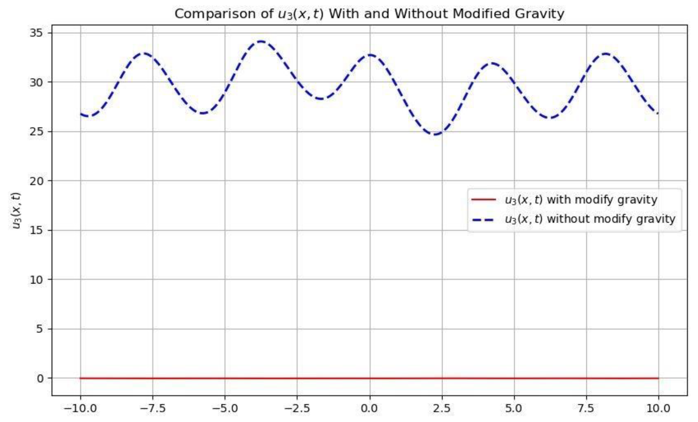
The effect of modified gravity caused the deep water at third layer to be stratified and move with constant velocity. Without the impact of modified gravity the deep water at third layer is not stratified as shown, rather there is an oscillatory motion with varying amplitudes.

Figure 9. The behavior of modified gravity on height in second layer of stratified deep water.

Figure 9. The behavior of modified gravity on height in second layer of stratified deep water.

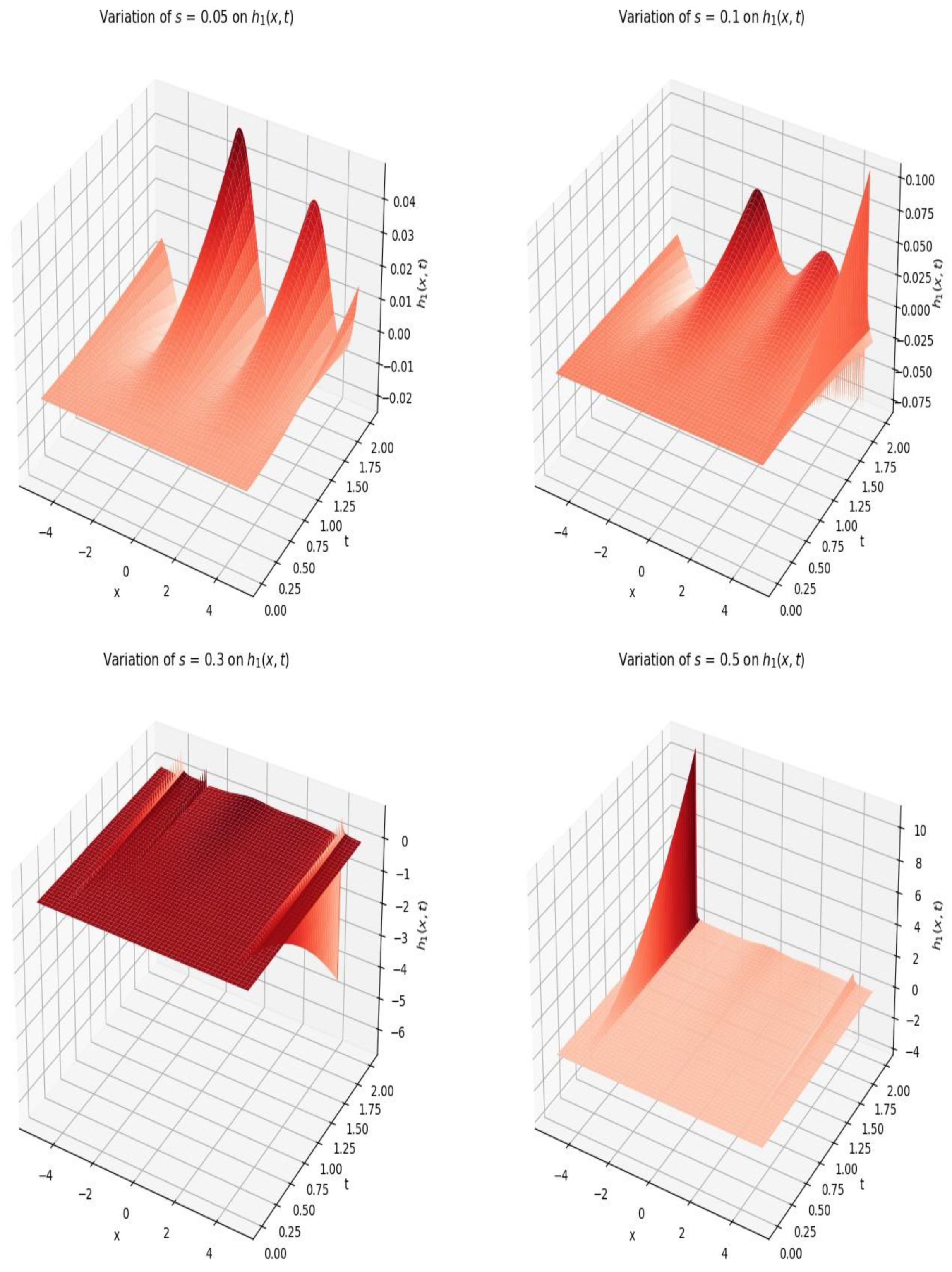
As result of gravity modification there is layering of water masses in vertical column leading to stratified height of the column. There is stratification on the first layer at different values of $\beta =0.05,0.1,0.3and0.5$

The clear impact of gravity modification is shown in Figure 12 as variation in measure of strength on velocity at $\alpha =0.6283185307179586,\alpha =1.5707963267948966,\alpha =3.141592653589793,\alpha =6.283185307179586$ leads to more stratified columns.

Figure 10. The impact of measure of strength on velocity of the second stratified column.

Figure 10. The impact of measure of strength on velocity of the second stratified column.

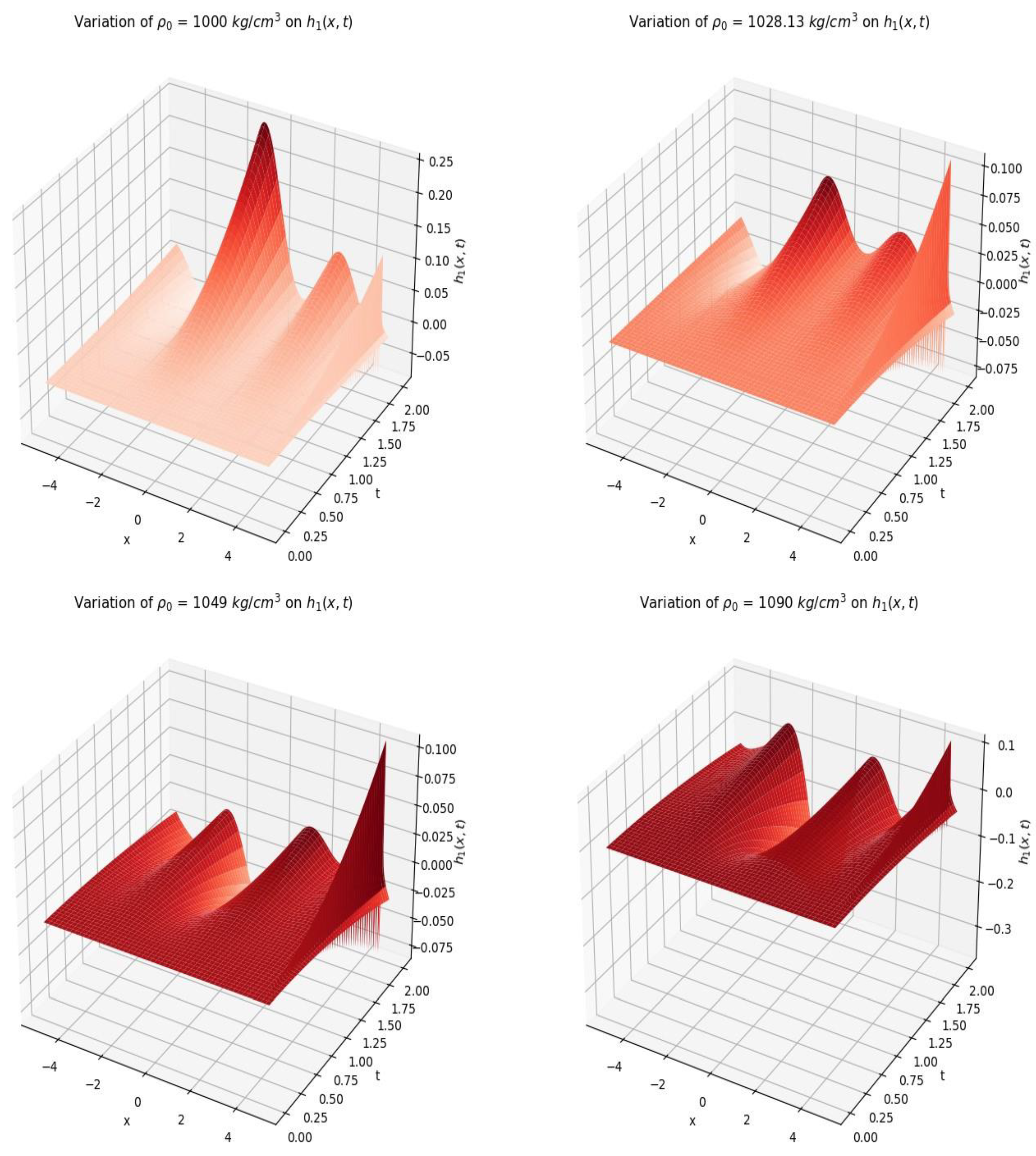
The impact of density on stratification under modified gravity is shown on Figure 13 as there are various degree of stratification at $\rho =1000kg/c{m}^3,\rho =1028.13kg/c{m}^3$, $\rho =1049kg/c{m}^3$, $\rho =1090kg/c{m}^3.$ Owing to modified gravity there is stratification in first layer. This shows that density variation leads to gravity modification which equally causes stratification.

Figure 11. The density variation leading to more stratified columns.

Figure 11. The density variation leading to more stratified columns.

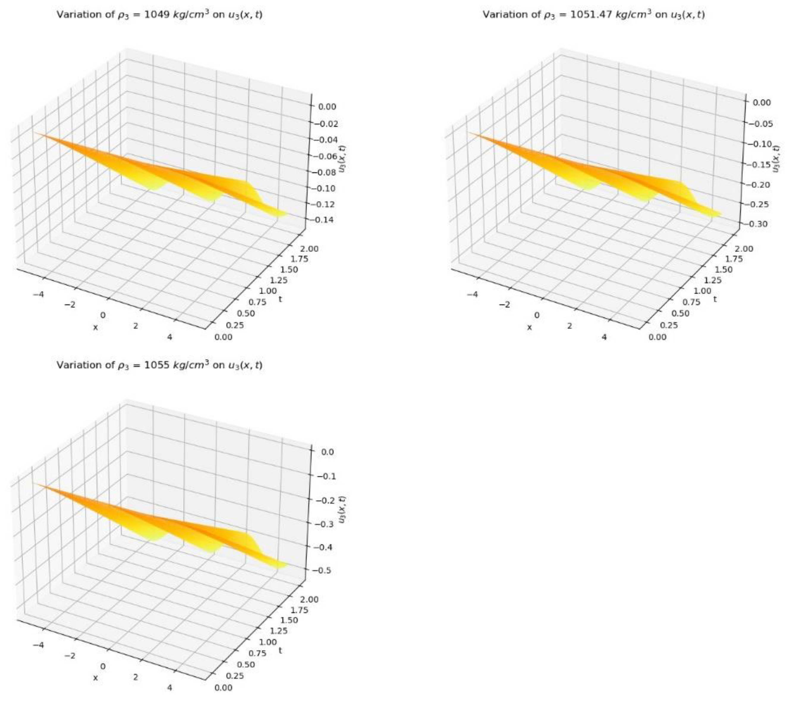
The effect of variation density with velocity in the third layer is shown in Figure 14.

Figure 12. Variation of densities with velocities in third layer.

Figure 12. Variation of densities with velocities in third layer.

8. Conclusions

We have sufficiently shown that modified gravity and Coriolis effect are the major factors that facilitate stratification in deep water.

The nth dimensional model of stratified deep water equations under modified gravity and Coriolis effect can provide better insights in making accurate predictions on the dynamics of fluid motion in stratified systems. Its ability to take into account the effects of gravity and Coriolis force makes it a valuable tool for studying a wide range of phenomena in oceanography, meteorology, and other fields of interest. The model can improve our understanding of ocean dynamics: By studying the behavior of stratified deep water under modified gravity and Coriolis effect, researchers can gain a better understanding of the complex dynamics of the ocean. This knowledge can be used to improve ocean models, which are essential for predicting ocean currents, waves, and other phenomena that can impact weather patterns, marine ecosystems, and human activities.

The model gives better understanding of the climate, and the behavior of stratified deep water under modified gravity and Coriolis effect captured in this model will provide a significant insight on global climate patterns for more accurate predictions of future climate change and help policymakers develop strategies to mitigate its impacts.

The model provides an enhance understanding of stratified deep water environments which are often rich in oil and gas resources. By studying the behavior of fluids in these environments under modified gravity and Coriolis effect, we can develop new techniques for oil and gas exploration and extraction, leading to more efficient and cost-effective methods for extracting these valuable resources.

The model helps in advancement of underwater robotics. The study of nth dimensional model equations of stratified deep water under modified gravity and Coriolis effect, lead to advancements in underwater robotics. It enhances our understanding in developing robots that can operate in deep water environment.

In conclusion, this model provides researchers with opportunities to explore and study the ocean in ways that were previously impossible, leading to new discoveries and insights into the ocean's depths and its stability.

References

- Abd-el-Malek M. B. and Helal M. H. (2009). “Application of the Fractional Steps Method for the Numerical Solution of the Two - Dimensional.
- Abd-el-Malek M. B., Badran N. A. and Hassan H. S. (2007). “Lie-Group Method for Predicting Water Content for Immiscible Flow of Two Fluids in a Porous Medium,” Applied Mathematical Sciences, Vol. 1,No.24, pp. 1169-1180.
- M. de Boer, A. J. von der Heydt, and M. K. M. de Ruijter (2020),"Deep water mass formation and circulation in the North Atlantic: A review of recent findings" by Oceanography, 33(1), 32-40.
- Chae, D.: Note on the Liouville-type problem for the stationary Navier-Stokes equations in R3. J. Differ. Equ. 268, 1043–1049 (2020). [CrossRef]
- Charney J. G. (1948), on that scale of Atmospheric Motion. Academic Press, New-York, 1982.
- Chen, R.M., Fan, L., Walsh, S., Wheeler, M.H.: Rigidity of three-dimensional internal waves with constant vorticity. J. Math. Fluid Mech. (2023). https://doi.org/10.1007/s00021-023-00816-5 6. Constantin, A.: On the deep water wave motion. J. Phys. A 34, 1405–1417 (2001). https://doi.org/10. 1088/0305-4470/34/7/313.
- Constantin, A., Kartashova, E.: Effect of non-zero constant vorticity on the nonlinear resonances of capillary water waves. Europhys. Lett. 86, 29001 (2009). https://doi.org/10.1209/0295-5075/86/29001 8. Constantin, A.: Nonlinear Water Waves with Applications to Wave-Current Interac tions and Tsunamis. CBMS-NSF Regional Conference Series in Applied Mathematics, Society for Industrial and Applied Mathematics (SIAM), Philadelphia, PA 81, (2011). https://epubs.siam.org/doi/book/10.1137/1.9781611971873.
- Constantin, A.: Two-dimensionality of gravity water flows of constant non-zero vorticity beneath a surface wave train. Eur. J. Mech. B, Fluids 30, 12–16 (2011). https://doi.org/10.1016/j.euromechflu.2010.09.008 10. Constantin, A., Ivanov, R.I.: Equatorial wave-current interactions. Comm. Math. Phys. 370(1), 1–48 (2019). https://doi.org/10.1007/s00220-019-03483-8.
- Durran D. R. (2010). “Numerical Methods of Wave Equations in Geophysics Fluid Dynamics,” Springer-Verlag, New York.
- Escher, J., Matioc, A.V., Matioc, B.V.: On stratified steady periodic water waves with linear density distribution and stagnation points. J. Differ. Equs. 251(10), 2932–2949 (2011). [CrossRef]
- "The impact of climate change on deep water masses and ocean circulation: A review" T. M. Joyce, D. W. Waugh, and R. M. R. Jensen (2020), Climate Dynamics, 55(3-4), 735-754.
- Le Veque R. (2004). Finite Volume Methods for Hyperbolic Problems.
- Liu, M., Park, J. & Santamarina, J.C (2024). “Stratified water columns: Homogenization and interface evolution. Sci Rep 14, 11453. [CrossRef]
- Martin, C.I.: Some explicit solutions to the three-dimensional water wave problem. J. Math. Fluid Mech. 23(2), 33 (2021). [CrossRef]
- Martin, C.I.: On flow simplification occurring in three-dimensional water flows with non-vanishing constant vorticity. Appl. Math. Lett. 124, 107690 (2022). https://doi.org/10.1016/j.aml.2021.107690 39. Martin, C.I.: Liouville-type results for the time-dependent three-dimensional (inviscid and viscous) water.
- Mbah G. C.E . and Udogu, C. I. (2015) Open Channel Flow Over A Permeable River Bed Open Access Library Journal, 2, 1-7. [CrossRef]
- Martin, C.I.: Resonant interactions of capillary-gravity water waves. J. Math. Fluid Mech. 19(4), 807–817 (2017). [CrossRef]
- Nnamani Nicholas Topman and G.C.E Mbah (2024), Mathematical Modelling of Geophysical Fluid Flow: The Condition for Deep Water Stratification. [CrossRef]
- N.N Topman, G.C.E. Mbah, O.C. Collins and B.C. Agbata (2023). An application of Homotopy Perturbation Method (HPM) in a population. Volume 6, Issue 2 (Oct.-Nov.), 2023, ISSN(Online): 2682-5708.
- Pedlosky J. (1987). “Geophysical Fluid Dynamics,” Springer, New York.
- Pedlosky,J. (2003). Waves in the ocean and atmosphere: Introduction to wave Dynamics. Springer.3.2.4.
- Ponte R.M (2021). Deep water stratification and impacts on ocean currents and climate.
Figure 1.
Stratification in three layers under modified gravity and coriolis effect.
Disclaimer/Publisher’s Note: The statements, opinions and data contained in all publications are solely those of the individual author(s) and contributor(s) and not of MDPI and/or the editor(s). MDPI and/or the editor(s) disclaim responsibility for any injury to people or property resulting from any ideas, methods, instructions or products referred to in the content. |
© 2025 by the authors. Licensee MDPI, Basel, Switzerland. This article is an open access article distributed under the terms and conditions of the Creative Commons Attribution (CC BY) license (http://creativecommons.org/licenses/by/4.0/).
Copyright: This open access article is published under a Creative Commons CC BY 4.0 license, which permit the free download, distribution, and reuse, provided that the author and preprint are cited in any reuse.