Submitted:
02 May 2025
Posted:
06 May 2025
You are already at the latest version
Abstract
Distinguishing human written text from machine generated text is a widely studied topic. In our approach we intend to apply this to purely academic text, and compute Vietoris-Rips up to H2 to produce persistence diagrams which we can statistically analyze. We contribute a classification process with promising success rates. Later, we analyze the transformer structure using Alpha complex filtration.
Keywords:
n/a
; topological data analysis
; alpha complexes
; vietoris-rips complexes
1. Introduction
As AI tools become more ubiquitous, there is concern they may be used in inappropriate contexts. Some studies suggest that the cognitive offloading from using AI tools hinders critical thinking skills [1]. In academics, therefore, use of AI tools may impede learning. Identifying the use of machine-generated text in academic writing could help combat this harmful phenomenon.
Existing research on identifying machine written text usually focuses broadly on all types of text and uses machine learning models for classification [2]. Machine learning algorithms for identifying academic AI generated text in particular have also shown success [3].
Topological data analysis (TDA), on the other hand, has been used to study the structure of text and embeddings in many interesting ways. For example, differences in the structure of languages used to write the texts [4], differences between adult writing and children’s writing [5] and much more [6]. Applying TDA to the task of distinguishing machine written text versus human written text has also already been investigated [7], though on a generalized data set. Use of TDA to identify academic papers with fabricated results has also shown success [8]. We aim to expand on this by using topological data analysis to study academic writing; in particular, we analyze abstracts from published papers, and use novel metrics with simplicial complex filtrations to evaluate the topological differences in structure between human written abstracts and machine written ones.
1.1. Methodology
We will use two different embedding types to represent our data, each operating on a per-sentence level. First, we use the simple Bag of Words (BoW) embeddings, which gives a representation of which words were used in a given sentence out of all the words in the text. Next, we generate embeddings using Sentence-level Bi-directional Encoder Representations from Transformers (SBERT) to represent complex inter-mixing of context that is not represented well by simpler vector embeddings such as BoW. We use filtrations within the topological space induced by our metrics to generate Vietoris Rips simplicial complexes. The final topological output is persistence images, which are statistically modeled using two methods. Finally, we invoke our model to classify test cases and evaluate success against the known classification.
1.2. Manual Evaluation of Data
Our selected dataset from Hugging Face [9] took a sample of 10,000 published research papers and captured their title and abstract. From these, a set of machine-generated abstracts was created using the GPT-3.5-turbo-0301 model, prompted by the original paper’s title and abstract length (as a target length for the machine generated version).
As a motivating example, we manually compare a selection of a human-written abstract and the associated machine-generated abstract. The two abstracts below are both associated with the title 4d Gauge Theory and Gravity Generated from 3d Ones at High Energy. First we look at the human written abstract with an eye for any notable syntactic features:
Dynamical generation of 4d gauge theories and gravity at low energy from the 3d ones at high energy is studied, based on the fermion condensation mechanism recently proposed by Arkani-Hamed, Cohen and Georgi. For gravity, 4d Einstein gravity is generated from the multiple copy of the 3d ones, by referring to the two form gravity. Since the 3d Einstein action without matter coupling is topological, ultraviolet divergences are less singular in our model. In the gauge model, matter fermions are introduced on the discrete lattice following Wilson. Then, the 4d gauge interactions are correctly generated from the 3d theories even in the left-right asymmetric theories of the standard model. In order for this to occur, the Higgs fields as well as the gauge fields of the extra dimension should be generated by the fermion condensates. Therefore, the generation of the 4d standard model from the multiple copy of the 3d ones is quite promising. To solve the doubling problem in the weak interaction sector, two kinds of discrete lattices have to be introduced separately for L- and R-handed sectors, and the two types of Higgs fields should be generated.
Next we do the same examination for the machine-generated abstract:
In this paper, we investigate the relationship between 4d gauge theory and gravity that arises from 3d ones at high energy. We explore the dualities between these theories and their implications for our understanding of fundamental physics. Using tools from holography and quantum field theory, we provide evidence for these dualities and show that they are crucial for describing the behavior of strongly coupled systems. Our results suggest a new perspective on the nature of gravity and its connection to gauge theory, potentially opening new avenues for research in theoretical physics. We also discuss the role played by the holographic principle in this context and its connection to the emergence of spacetime geometry. Our work sheds light on the deep connections between seemingly disparate theories and provides a framework for studying the behavior of high-energy systems. Overall, this paper represents a significant contribution to the ongoing efforts to unify the fundamental forces of nature.
Our cursory comparison of the texts reveals several features. First, the human-written text has more direct references to proper nouns (i.e., referencing works by specific authors), as well as technical terms (“Einstein gravity”, “Higgs fields”, etc...). Furthermore, the machine-generated abstract uses more repetitive words as well as less technical jargon. Finally, the machine-generated abstract features more “stock phrases" such as “in this paper.” Overall, the machine generated text is simpler, with each word deviating but little from a normal non-technical vocabulary and each sentence offering little new vocabulary in relation to the rest of the abstract. The words of the human-written abstract are far more technical, and there are more sentences that do not directly relate to the others by vocabulary alone. Previous literature [10] has come to similar conclusions on AI-generated text in general. These facts can help inform us on what topological structures we might want to study to differentiate the two.
In particular, we can create a topological structure that represents the “similarity” between sentences in an abstract with all other sentences in the same abstract. We hypothesize that the structures will be “closer” in the machine written text and therefore generate different persistent homologies than in the human written text, to the extent that we expect a statistical analysis of persistence images to separate the two classes of texts and correctly identify if a persistence diagram came from a human-written abstract or a machine-written one.
2. Vietoris Rips-Based Evaluation
2.1. Text Embeddings
Text embeddings are a vector representation of a piece of text. The general construction is usually handled by models specialized in specific ways of representing features of the text. We have also decided to chunk the data into sentences, so our embeddings will each represent an entire sentence.
The simplest model, and our first choice of embedding is the Bag of Words (BoW) model. For BoW, an n dimensional vector is initialized that represents n unique words in a given abstract. From there, a count of each word, represented by the position in the vector, is made for all words in a sentence. This will give us a general representation of the layout of words across the abstract. In mathematical terms, if we consider to be the set of sentences in an abstract, the BoW model can be considered a map; .
The next model we chose is one of the most advanced, Bidirectional Encoder Representations from Transformers (BERT) [11]. We do not cover the specifics of the model here, electing instead to highlight a few key aspects of the resultant embedding. First, a key aspect is that synonyms and words with related meanings will be positioned near each other and given certain weights even if the specific word is not used. This helps the resultant vector be “closer” using traditional distance functions to other vectors that use the related words. BERT optimizes this even further and is able to use contextual information to identify use of homonyms, so even if the same word is used, if the contextual meanings are different, the resulting vector representation is not the same. Further, since we are operating on the set of sentences, we use Sentence-BERT [12] (SBERT) which further optimizes for sentence-level embeddings. Mathematically, we can consider where q is a constant number determined by the exact model used. For our purposes, we have selected a generalized pre-trained model “all-MiniLM-L6-v2” [13] which maps to a dimensional vector.
The code for each embedding type can be found in Appendix A.
2.2. Metric Selection
2.2.1. Cosine Similarity and Angular Distance
Cosine similarity has long been a popular measurement for comparing similarity of text documents [14]. In order to study the structure of texts based on how similar each token is to one another (since we posited earlier that the AI generated texts may be more self-similar than the human written ones), it makes intuitive sense to do our investigation within the metric space formed by this measure. However, the traditional definition, as defined in 1[15] where A, B are n-dimensional vectors, does not meet the definition of a metric
Notably, this is the cosine of the angle between two vectors, therefore the value is zero when they are orthogonal, so does not imply . More importantly, it does not follow the triangle inequality. This can be seen in a simple two-dimensional case with vectors , , and . , and , which then gives .
However, we can recover the angular distance measure from the cosine similarity by using 2:
Which gives us as a metric when A and B are normalized (i.e., , which can be achieved with normalization ).
Proof.
First we note for all x. Next, when , then . On the converse, when , then so . From the Cauchy–Schwarz inequality we know this holds if and only if . This can be further reduced if we take A and B only from the unit sphere (which can be achieved via normalizing), so when . Therefore we get a further refinement to 3
Considering points , we can take the plane containing all three points and consider it in . Then, we can write them using their angle, i.e., , and . Using a common trigonometric identity to write , our angular distance function is now equivalent to . Therefore,
so we see the property holds. Therefore 3 is a metric. □
A final step is to multiply by a factor of to normalize the output to fall within the segment , which has no effect on the validity of the metric. So our final metric becomes:
The overall flow of generating this distance from our data is depicted in Figure 1, starting with sentences from to ending up with our measure of distance in .
2.2.2. Experimental Composite Metric
We do not know up front which embeddings are best to capture the structure of sentences that will give the most topologically interesting views of the texts. One way to handle this scenario is to use a composite distance metric that incorporates multiple embeddings, with a weighting variable that we can tune to compare how certain weights affect the topology generated by the filtration. In essence, the function will map from the set , the collection of sentences to a distance in . Treating the different embeddings of the sentences as black box functions mapping from to where n is decided by the embedding, we can write them as . Taking two embeddings , , sentences , and some we can take a composite metric as
Proof.
Proof is a metric. We have already proved that is a metric. Therefore, for , we can see when ,
and when then which leads to . Next we see
Finally, for the triangle inequality,
Therefore, is a metric. □
For our purposes, we are using the composite metric on BoW and SBERT, so our metric in particular will be
The pipeline for fully calculating the composite metric is pictured in Figure 2.
2.2.3. Smoothing
As discussed in [16], a way of encoding basic structural information is to use “smoothing.” The basic idea is to force closeness for nearby sentences by taking an embedding for sentence ; A is a weighted average of the embeddings of the k closest sentences, i.e., . For our purposes, we chose , with weights and . The resultant comprised of the smoothed vectors still is a vector in for , therefore our metrics are still valid.
2.3. Method and Implementation
Since we have chosen distance functions that fully realize all properties of a metric, we are able to operate in a metric space, which is the basis of a certain topology [17]. We build simplicial complexes using Vietoris-Rips which consists of simplices at different filtration levels such that:
The diameter is determined by the distance, computed with the relevant metrics. Vertices are included at the first filtration be default since for any metric. Edges between vertices are added once the pairwise distance of the points fits within the filtration. Triangles are added once the last edge to complete it is added, and so on in higher dimensions. Running through with increasing filtration levels, we can determine the where a given first appears (known as its “birth”). A simplex may then join a chain with other simplices of the same dimension, until a homology is formed. Once that homology is absorbed into a simplex at a higher dimension at a certain filtration level , we mark that as the “death”. We then have the persistence interval for that homology from [, ]. We analyze these homologies in H0 (connected components), H1 (loops), and H2 (voids). Tracking these across the different dimensions shows tells us about the persistent homology. The algorithm [18] for calculating these birth/death pairs uses a boundary matrix from an ordering of the simplicial complexes based on the birth epoch of the simplices. The reduced form of this matrix reveals the persistent homologies, and also allows us to keep track of the chains involved.
In our case, we are running a Vietoris-Rips filtration per combination of embedding type, metric, and presence of smoothing or not for a given abstract. Given our limited compute power, we ran on 1000 abstracts (which involved two filtrations per abstract - one for the human version and one for the AI version) for each combination.
Our implementation is done in python and can be found at https://github.com/aguilin1/tda_ai_text_generation/blob/main/tda_ai_text_detection.ipynb. Simplices are built up by first evaluating the pairwise distance (using the chosen metric, in this case angular distance) between two embedding vectors. We track and label the simplices using an extended “frozenset” object that tracks the sentence included in that given simplex. These distances are then used to compute the simplices in 0 dimensions (just the sentences themselves), 1 dimensions (the edges between two sentences), 2 dimensions, 3 dimensions and 4 dimensions, where each simplex keeps track of the distance of the largest edge involved in its construction. From here, we iterate through each measured distance and create an ordered list of simplices by birth time. Then, we create a sparse representation of the boundary matrix and run the persistence algorithm. Set symmetric differences of indices are used to mimic addition in .
For speed, we also leveraged the python Ripser package [19] for evaluating persistence using the composite metric, which leverages a distance matrix calculated using the composite metric described above.
During the evaluation, we tracked the number of persistent members of H0, H1, and H2 (where persistent indicates they were not born and died in the same filtration). We took the average size across all abstracts in a given run and would expect to see different sizes between the human written abstracts and the AI generated ones. As seen in Table 1, there were slight differences, which does show the structures between human text and AI text generally were different.
3. Results
We present two representations of simplicial complex persistence and discuss their usefulness in this analysis. A major point of study is a statistical method to describe the topological structure of many abstracts as a group or groups and then classify test cases based on their adherence to a particular statistical description. Our main result shows that a linear statistical model can helpfully describe statistical difference between the topological structures of human or AI abstracts when embedded and measured using the encodings and metrics given above. This contribution serves as a preliminary, exploratory topological data analysis with numerical results which can be used as a lower bound on success, to be raised in future efforts.
3.1. Metric Values
Here we briefly revisit our hypothesis that structures formed by the vector embeddings from AI-generated abstracts will be “closer” to each other than those formed by embeddings from human-generated abstracts. Within a class of abstracts, AI or human, we found a remarkable diversity in the histograms of distances between the vectors under our metrics. Several examples are shown in Figure 3. Our hypothesis was not confirmed by smaller distance values in the AI-generated samples. Nevertheless, we show below in our classification section that the structures between classes are indeed significantly different—this is simply not revealed by the metric values.
3.2. Simplicial Complex Outputs and Their Transformations
The foremost measure of significance of a topological structure in a simplicial complex is persistence, meaning a measure of how long a feature lives after being born at some epoch of complex filtration but before being killed by a higher-dimension feature in another (possibly later) epoch. Typically, those features which die quickly are insignificant to the underlying structure of the data. For example, if the data has an inherent geometric ring-like structure with a large hole in the center, the hole in the center should live much longer than a hole triangulated between three neighboring points on the diameter of the ring. There are many different measures and visualizations for persistence, and we present two here. Our code tracks and averages the number of elements which have nonzero lifetime in each dimension which gives a rude measure of how many important topological features an average abstract has under our embeddings and metrics. See the tabulated results in Table 1.
These results show that there are a significant number of connected components in each abstract, probably corresponding roughly to the number of sentences in the abstract. There is roughly 1 cycle in each abstract. The 3-dimensional voids are interesting because, although they occur very infrequently, they clearly occur at different rates in AI abstracts ( in 30 abstracts) than in Human abstracts ( in 21 abstracts). This difference is a contributing factor to the better classification scores in H2 than in H0-H1. These scores are discussed below.
3.2.1. Persistence Diagrams
A persistence diagram is a simple and effective representation of persistence. The data on a persistence diagram is (x,y) pairs corresponding to the birth epoch and death epoch of a certain homological feature during the filtration of a simplicial complex. These birth and death epochs are found by a running reduction of a boundary map matrix that is built up as the filtration steps through each epoch. Naturally, all points on a persistence diagram are on or above the x=y (birth = death) diagonal, and the vertical distance of a point from the diagonal is the lifetime or persistence of that feature. Various simplifications and clarifications are often used, such as omitting points on the diagonal, coloring differently points of different dimensions, and including a horizontal “infinity” line above the maximum epoch value to gather undying features.
The strongest benefits of the persistence diagram are the ability to show multiple dimensions of features in a single visualization and to identify precisely the persistence of features. Depending on the complexity of filtration implementation and the size of the data, a point on a persistence diagram may be explicitly related to the textual feature it represents. This may allow better analysis of the meaning of a persistent feature. Persistence diagrams are stable to small changes in the data, and are also pairwise comparable using various distance measures such as bottleneck distance[20].
3.2.2. Persistence Images
A more recent development is the persistence image, which similarly promises stability under noise in the data. This is a key assertion, because persistence of a feature without stability may not be meaningful. Posed as a question, is a feature truly persistent if a small amount of noise causes its lifetime to decrease significantly? To that end, Adams et al. have shown that, like persistence diagrams, persistence images are stable in the presence of noise[21].
Furthermore, a persistence image is a vector representation of a persistence diagram (see Figure 4). There are two major implications of this statements. First, persistence images are well-suited for machine learning applications, or more broadly, well-suited for analysis of large sets of persistence diagrams. Recall that persistence diagrams are best compared pairwise rather than as a large set. Second, persistence images can be produced directly from the persistence diagram data, which is a set of birth-death pairs for each dimension. One disadvantage of persistence images is they are exclusive to one dimension, meaning that a persistence diagram for up to dimension 2 can have 3 different persistence images.
Persistence images are formed as follows. First, data is transformed by converting birth-death points into birth-lifetime points and applying a weight function to them. The weight function is often linear with the lifetime so that higher lifetimes are emphasized. The next step is to sum over all the weighted points times a Gaussian probability distribution, resulting in a persistence surface. Then, by integrating over a specific pixelation of that surface, the persistence image is created and is visualized as a heatmap of the discrete statistical distribution of persistence versus birth epoch. Because the persistence image is pixelated, it can be flattened into a vector format as mentioned above and compared to other persistence images of the same resolution. There are other methods of binning the birth-death pairs and applying statistical distributions to persistence diagrams. We use persistence images in our analysis for their understandable graphical representation and tunable mathematical characteristics[21]. , The reader may refer to the Appendices for example persistence images from each embedding type, smoothing choice, and metric choice.
A critical step in the analysis is tuning the variance, or width, of the Gaussian PDF used in creating the persistence images. For H0, all the points are on the vertical axis since they are all born at zero, so the x-variance should be very close to zero. For all dimensions, the variance should be small enough that important features are not washed out by overly wide Gaussian surfaces, but large enough that some smoothing is achieved. Our implementation uses a pixel size of 0.05 to make 20X20 images and uses a Gaussian variance of 0.001 to distribute each persistence diagram point over several pixels in the image. For reference, the Gaussian curve will reach approximately zero at about +/- 0.15 (three pixel widths) away from the mean.
3.3. Statistical Modeling and Test Case Analysis
We generated two statistical classification models to operate on test-case abstracts and determine whether each abstract was human-created or ai-generated. The approaches were linear regression and basic binning, and both were largely successful relative to their sophistication level. Training of complex classification models was outside the main scope of this study, so we did not attempt to implement any machine learning models for classification.
3.3.1. Regression Models
We implemented a simple linear regression model first. In this approach, for each of the 3 dimensions, our code randomly took 80% of the images from the full set of flattened persistence images and fed them as training data into a linear regression fitting tool. The remaining 20% of images were used as test data. Each run had a minimum of 300 images (100 abstracts) and the largest run included 3000 images (1000 abstracts) of each class. The regression model classified test cases at all dimensions from zero to two at a best success rate of 70% or greater. The numerical results tabulated below in Table 2). From this we noted the following:
- A linear model does capture the statistical relationship between the topological structures of human-created and AI-generated texts under the chosen embeddings and metrics, and
- Overlap in the bell-shaped PI representations of a homology for the two classes probably corresponds to errors in classification for any model
- No assertion can be made, based on these results, about the effectiveness of a linear model on similar data under different choices of embeddings and metrics.
With the linear regression serving as an informative and successful first attempt, we also implemented support vector machine (SVM) model using a nonlinear radial basis function (RBF). The RBF kernel maps the (presumed) nonlinear data into a higher dimensional space where it can discriminate linearly between classes (see explanation here). In the scikit-learn Python implementation, the code looks very similar to the linear model, with one critical change: there are two parameters to adjust to tune the SVM model. There is an additional iterative training suite that can find the best parameters, so we first ran all of the test data through through that suite to determine the correct parameter choices. Upon inputting those optimal parameter values into the main code and running the model on test cases, the model score dropped to approximately zero. We also frequently obtained negative scores, which according to the documentation are possible because the score is not a success rate but rather is a coefficient of determination with a maximum of 1.0 and no minimum since the model can be arbitrarily poor.
3.3.2. Binning
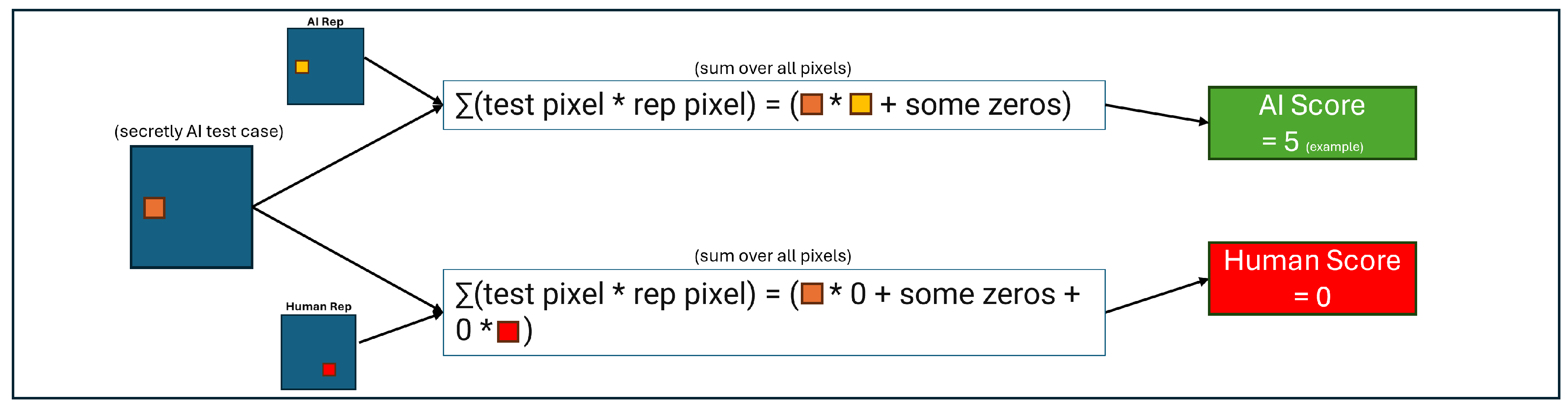
Our final approach to classification was to sum by pixel over all the randomly-selected training persistence images in a class (AI or human) and normalize the result by the sum over all pixels in the summed image. The result is a persistence image with contributions from every training image, but with a total pixel value sum of 1. This mimics a discrete PDF, and we denote it as the “class representative image” as in Figure 5. Then, for a randomly selected test persistence image, we took the dot product with each class representative image. The larger of the two resultant values determined the classification of the test image. Over the whole set of test images for a given embedding and metric, we summed the successful classifications and divided by the total number of test images to obtain a score.
Figure 5.
Process for generating class-representative persistence images from the body of randomly selected training persistence images for each class.
Figure 5.
Process for generating class-representative persistence images from the body of randomly selected training persistence images for each class.
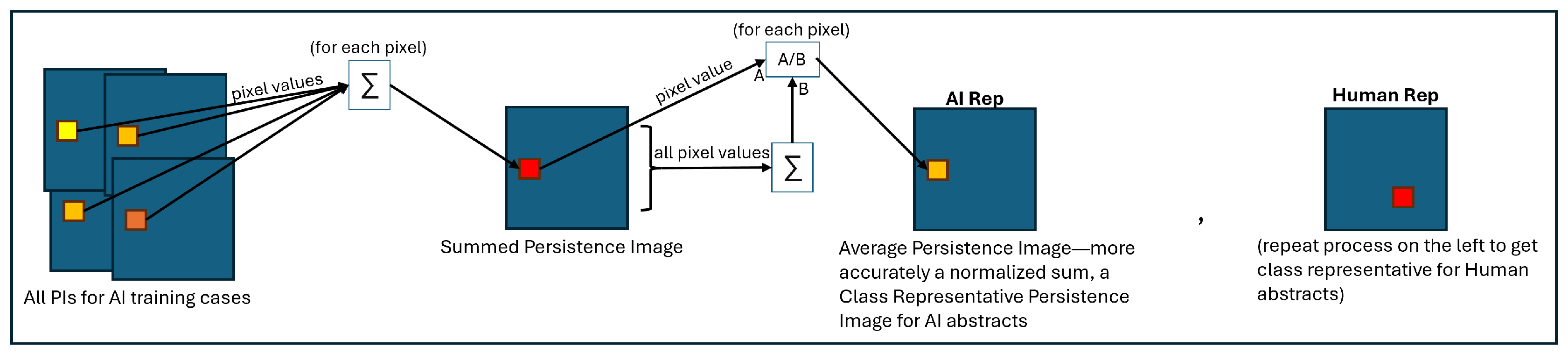
Figure 6.
Process for classifying a randomly selected test persistence image using the class-representative persistence images.
Figure 6.
Process for classifying a randomly selected test persistence image using the class-representative persistence images.
3.3.3. Test Case Classification Results
In Table 2 we show the classification score for each tested combination of embedding, metric, classification tool, and dimension. Note that the best results for every dimension are 70% or higher. These numbers are for 1000 total abstracts split randomly into 800 training cases and 200 test cases. Because of the averaging performed on the class representative persistence diagram in each dimension, the results are not highly sensitive to slight changes in the number of samples.
4. Discussion
Based on our results, we achieved moderate success in identifying AI text from human text only using topological features. This shows that even simple embeddings that track small bits of information (such as count of words for Bag of Words) can be used to analyze the topological structure of short, academic texts and find meaningful differences. We are also optimistic that further tuning of each step in the algorithm chain would further increase the classification scores of our model.
Generally the worst performance came from using the Bag of Words embedding with smoothing. This may be because averaging out word usage across neighboring sentences likely flattens out the whole abstract into indistinguishable sentences. On the other hand, the best performance came from the SBERT embeddings. We can also notice that the composite metrics that were weighted toward SBERT did better than the ones weighted toward BoW. This likely indicates that SBERT is capturing more than just word choice, and the differences in meaning across sentences is a stronger differentiator of AI text versus human text. SBERT also showed the biggest difference in the size of the homologies across human text and AI text, showing that the topological structures were quite distinct.
However, there may be stronger links and even more distinct topological structure available if we were able to represent more information about the text in our embeddings. For example, our embeddings generally do not capture sentence structure (arrangement of the different parts of speech in certain orderings), but that may be a feature that is very different between AI text and human text, and result in more distinct topological structures. Additionally, we relied on pre-trained encoders. These are trained on a large set of most-common words, and academic language may be underrepresented in that body of words. These aspects, as well as investigating filtrations based on Alpha complexes are explored in the latter half of the paper.
We also observed that linear regression consistently outperformed binning in H0, but the reverse happened in H1. We were able to most consistently achieve good classification scores with our variety of embedding and metric types using the H0 data. An interesting experiment would be to classify based on the predicted classifications from each dimension, in hopes that the redundancy would provide better results. For example, how often will an Human abstract be classified correctly if the H0, H1, and H2 classifiers all predict it is Human? What if one dimension has a dissenting prediction? This sort of probabilistic analysis would be very informative and should raise the confidence level of any tool created on a similar architecture to ours.
For most choices of a pixel size, our persistence images were either a line of values (H0) or a Gaussian-weighted blob of various values centered at some location in the image. We believe the success of the linear regression model and binning method depended on this fact and that the presence of additional “hot” areas on the persistence images would have destroyed the usability of linear regression. For example, with only one hot area per persistence image in a given AI or human class, the regression model could simply draw a line between the heat center for an average AI image and the heat center for an average human image. The results were not perfect for several reasons. First, there remained some overlap in hot areas across classes as shown in Figure 7; this means that some test case points scored very similarly for each class for both linear regression and binning. Second, experimenting with very small persistence image pixel sizes and Gaussian variances showed that the data did not always fit in a single hot area. For instance, the H2 persistence diagrams under SBERT embeddings with a very small pixel size showed two neighboring hot spots. These reasons contribute to imperfect test scores, but linear regression and binning were still able to discriminate between classes at each dimension on average.
5. Transformer Investigation
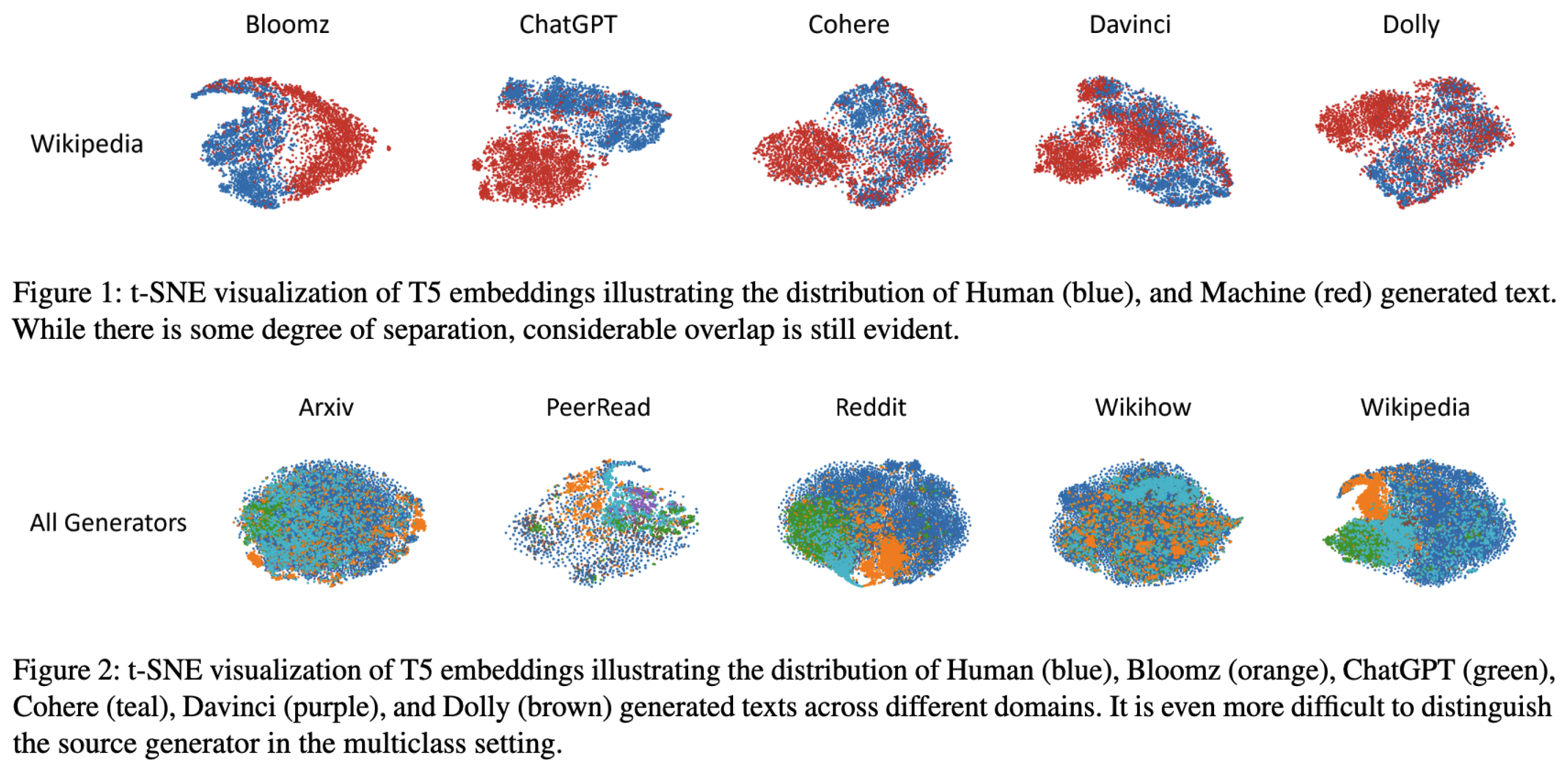
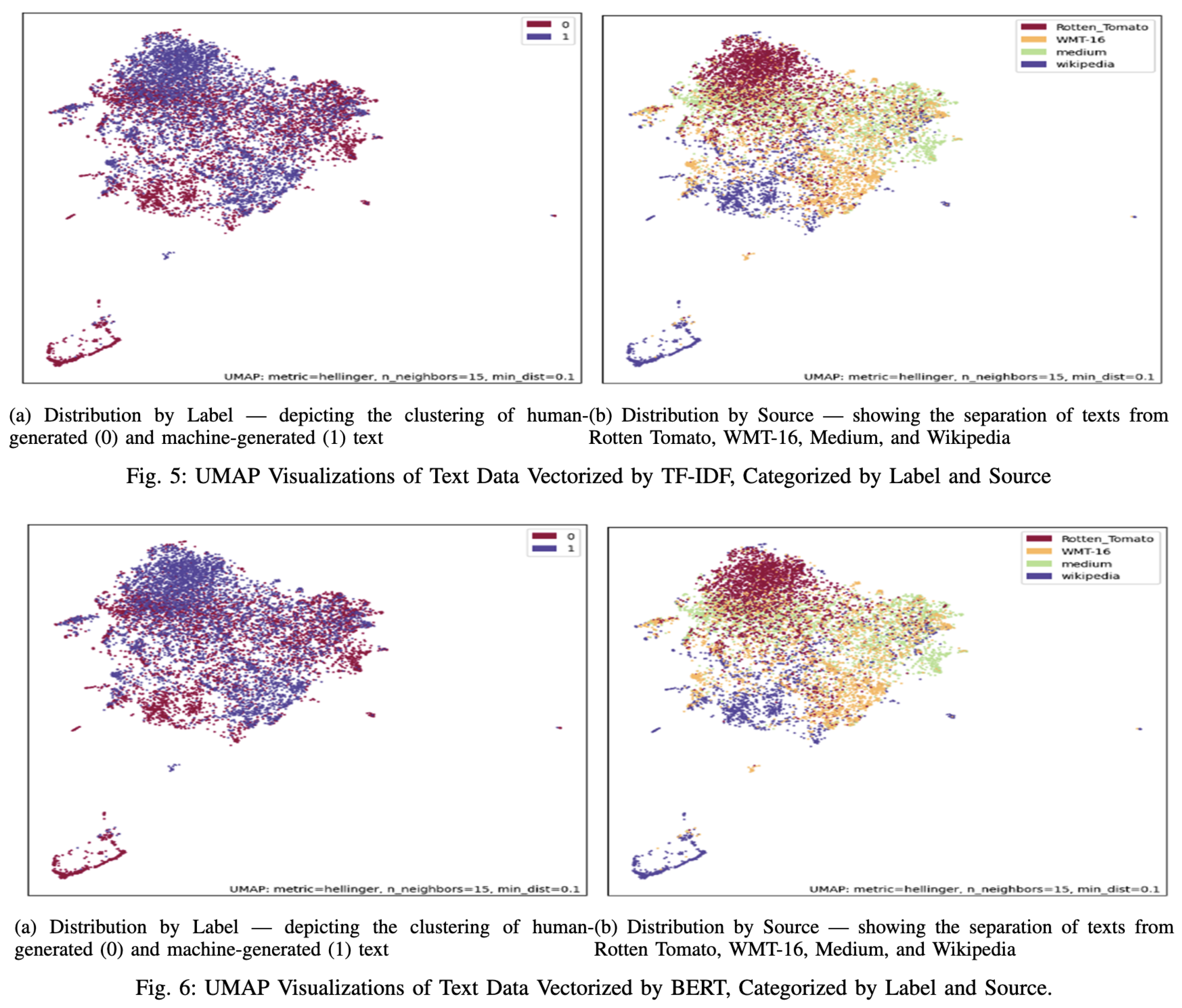
Transformers are not yet fully understood. Most of the Generative-AI models hinge upon various Transformer model variations. We intend to use topological analysis to understand impact of embeddings generated by encoder-decoders layers on over-all efficacy of AI/Human text generation detection methods. Today we do not see any research in this area that goes beyond common UMAP, t-SNE based clustering [22], generating outcome as following, while very useful but giving no information about how various representations could have changed this separation.
We, in our-approach, will traverse Transformer architecture and generated BERT homology, back and forth to gain insight into what changes in transformer drive actual separation of data. This is a poorly understood problem as Bataineh et. al. [2] correctly point out BERT embeddings can not be explained simply. Key hinderance encountered in deploying AI, in any regulatory settings that requests to Right to Explanation.
With our limited compute budget, we do not aim to go deeper in to the complex topological multidimensional spaces beyond 4 dimensions.
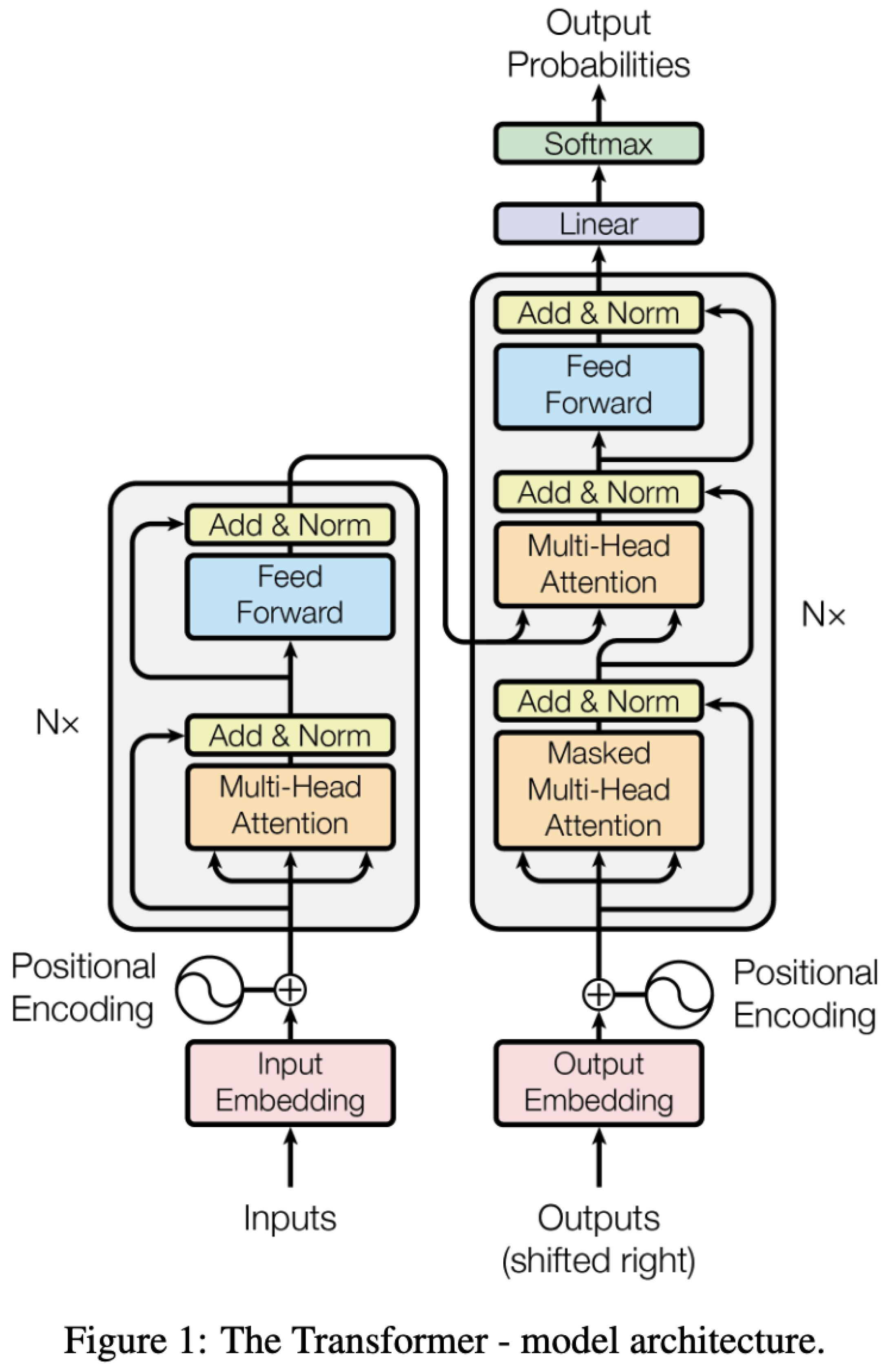
Transformers use sin/cosine functions of different frequencies to encode position of various tokens in a paragraph (see Input Embedding Sublayer in the Transformer Model) (as we are using 200 word fixed size paragraphs). This representation will be very different from BoW, TF-IDF representations as these representations have no context and position is essentially a linear function. We want to use topological analysis to understand transformers.
5.1. Why Do We Care About Embedding?
BERT Embeddings can not be explained easily [2] Vast amount of published research using BERT embeddings has relied upon H0/H1 homology information from Vietoris-Rips like coarse grain simplicial complexes which are not suitable for such analysis as it includes all simplices based on simple pairwise distance criterion. Many have declared that "Hidden state representation remains topologically simple throughout training" [23]. This can not be farther from truth. Others have also verified this thus making it harder to dispute. We present bert-base-uncased transformer model’s topological analysis for "[CLS] " token showing all 13 layers (12 + 1 classification). We also share Jupyter Notebook VietorisVsAlpha.ipynb that anyone can run to verify this for their own transformer datasets (we have used tda-scikit as reference).
Persistent Homology and Transformers [24] Transformers carry fine grained topological structures that can not be utilized using coarse grain topological data analysis tools and even with extensive filtration, complexes collapse early and often are unable to provide any information about persistent homology that is representative of underlying topology [25]. This is the reason, Biological topological data analysis almost never uses Vietoris-Rips complexes.
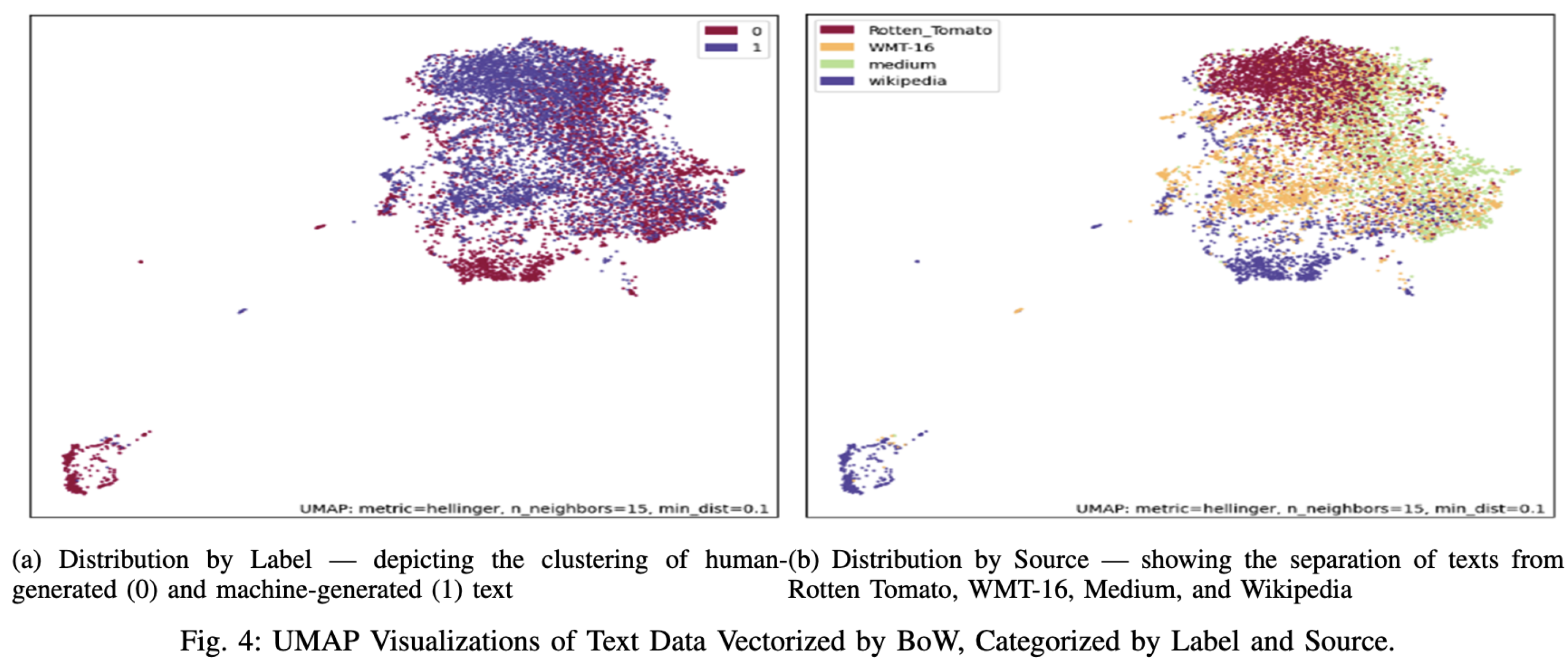
Many topological analysis approaches UMAP and Machine Learning based classification algorithms such as XGBoost and Random Forest fail, when algorithms implementing these models are fed Bidirectional Encoder based embeddings [2], as BoW (Bag of Words), TF-IDF do not carry context information embedded in encodings coming from Transformers so machine vs human generated data can discern features to lock on to, much more easily. XGBoost, Random Forest based classification methods take upto 20 percent hit in classification accuracy as they encounter BERT based vector representations.
See UMAP based clustering failing to separate Human vs AI text using BERT representation [2], while it was successful for BoW and TF-IDF.
We intend to connect transformers to TDA analysis by not replacing, any underlying representations, along the way. We want to be able to go back to transformers, generate new embeddings if needed and have this data fed to code, using various metrics (way to separate points), filtrations, and simplicial complexes such as Vietoris-Rips and Weighted Alpha Complexes generating homology (H0, H1, H2 etc..), persistence diagrams as these features come to life and disappear based on filtration values (radius of balls deployed) reflecting end to end connection. Our hope is that this approach will shed more light into inner-workings of Transformers.
5.2. Challenges
Topological data analysis of transformer generated text is not new. However almost all approaches run into following walls.
5.2.1. Text Vector Representation and Tool Effectiveness
Representation changes outcome. Using BERT, XGBoost takes 20 percent hit in performance. BERT representation can be changed to vectors of 50 integers, 80 integers or 200 integers, reflecting the complexity of implementation (6 mor more layers, heads (single/multihead), residual connections bypassing layers etc. are deployed). We will use nanoGPT with pre-loaded weights for our experimentation, changing only the embeddings (set to fixed size 50) going in as input embedding thus gaining insight into the role of Encoder-Decoder stacks.
5.2.2. Non English Text
We are using this as input to transformers to see how embedding separation changes for a given manifold deploying certain topology as semantic changes.
5.2.3. Shorter Text (1000 Characters or Less) Fails Detection - Analysis of Features Using Explanable Models from SHAP [26]
Plagiarism detection tools can be fooled simply by not using certain kind of phrases by detecting how Perplexity and Burstiness is modeled in underlying LLM implementation. By using shorter phrases, writer can control how complexity and burstiness is manifested in text generation thus changing BERT representation, thus forcing AI generated BERT vector to land close to human generated text. We hop to overcome this challenge by going deeper into the topological space by also looking at H1 and H2 homology as well as homology generated by 2 simplicial complexes (Alpha and Vietoris-Rips).
SHAP uses learnings from co-operative game theory to detect which feature in any AI model are playing any role in final assignment of classification using local-accuracy and missingness. SHAP assigns each feature a (-4,4) value tracking each prediction tracking additive feature attribution methods (https://github.com/shap/shap. SHAP provides an explanation model to explain predictions performed by any model based on its underlying features and then SHAP uses co-operative game theory theorem using local accuracy and missingness properties while arguing that consistency property becomes redundant in context of additive feature attribution explanation context for prediction outcomes using Shapley Values).
Key mathematical ideas for additive feature attribution (we should see these in our topological analysis as well) are:
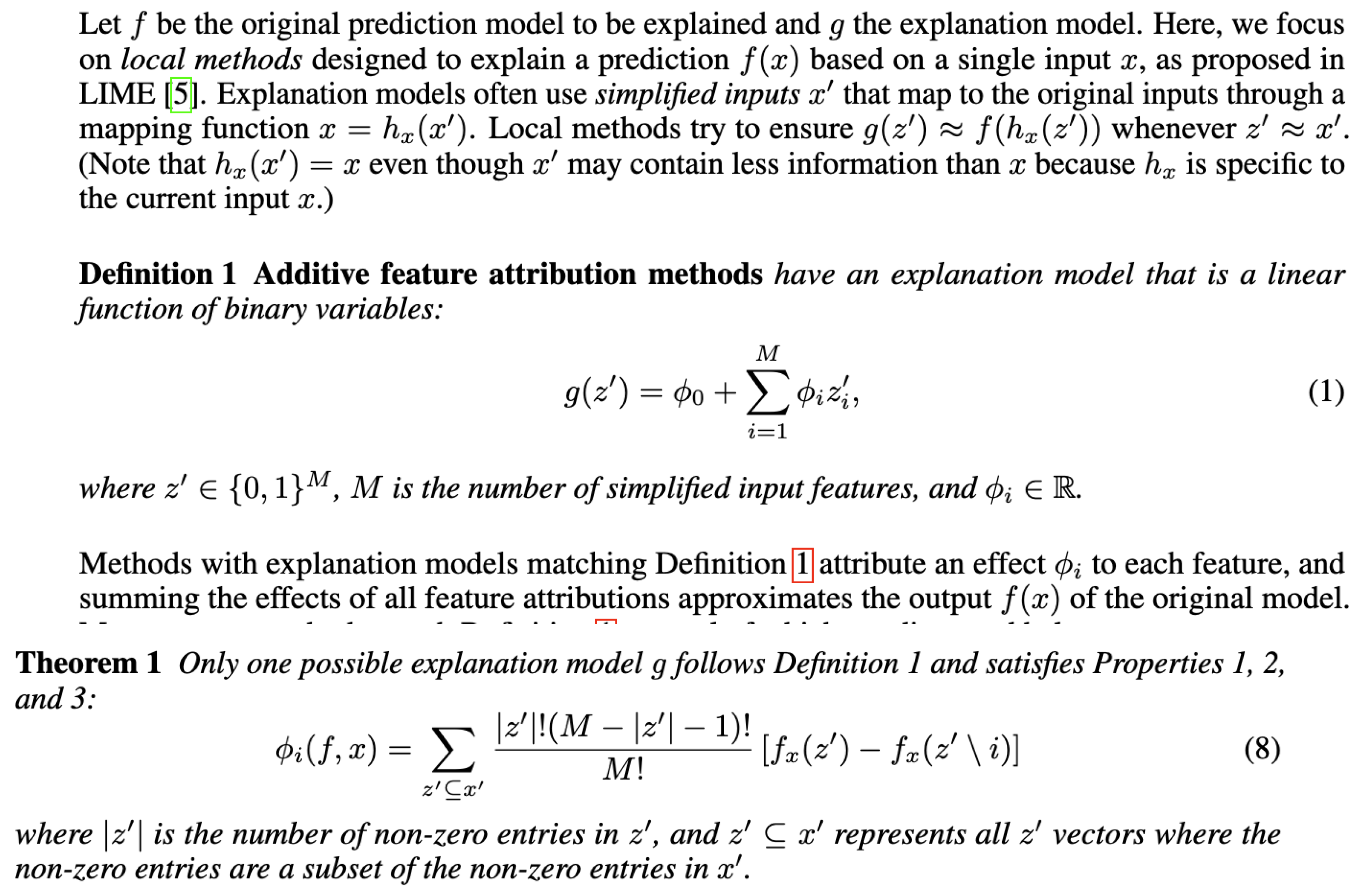
See SHAP paper [26] for further details.
5.2.4. Fine-Tuned Generative Models
State of the model fine-tuned to write briefings for lawyers are designed to mimic humans. These models use boiler-plate language which is almost identical to what is used by lawyers in large law firms as they themselves have these boiler-plate templates for junior lawyers to copy. Such text evades AI vs Human Text generation often. We do not have access to any data-set representing this so we will leave our analysis with this caveat open.
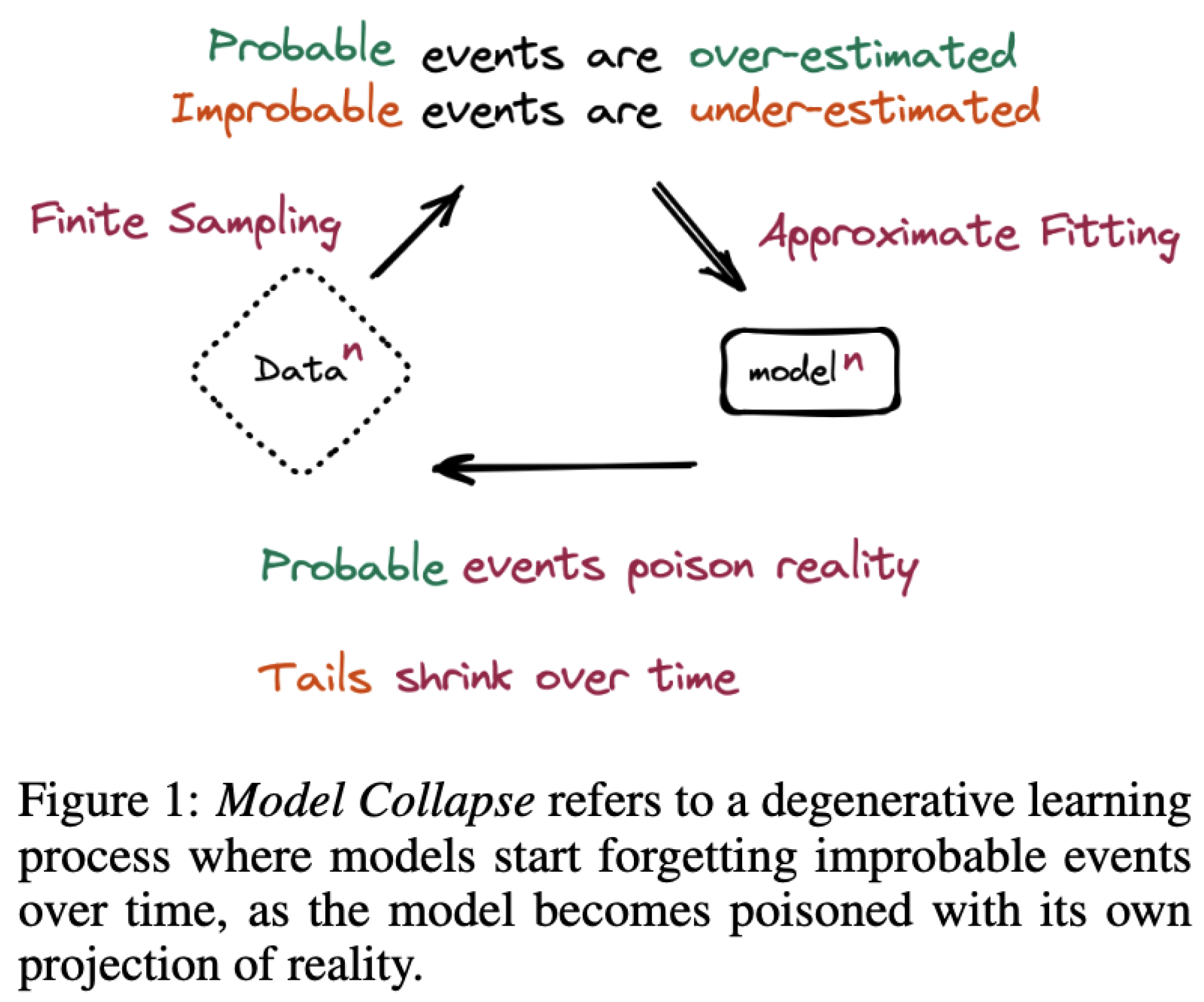
5.2.5. Curse of Recursion
Ilia Shumailov et al. [27] argue that lot of text written by humans in online articles is already generated by LLMs as revised text correcting errors or setting an alternate tone that is different than how original author generally writes. Using this text as “human generated” text for training is causing models detecting difference between LLM text and genuine human text harder and harder. This is leading to "Modal Collapse". This is attribute to Diffusion of features creeping from text that dataset thinks is human generated, but it may not be so... (GAN inspired) (The Curse Of Recursion)
5.3. Methods - Coaxing Data to Our Small Complexes
We share our Jupyter notebook that processes data along with methods to reduce dimensionality of BERT vector representations of 768 bytes down to 50 bytes using Subspace Embedding [28].
We can either iterate on a Matrix representation as highlighted below or just pick one shot-representation picking 50 winners from 760 byte representation allowing 25 largest (+ve) values and 25 (-ve) smallest values.
We want to keep this projection separate from our metric calculations defining topology as then we may not be able to separate out impact on analysis of separation coming out from topology vs our inability to process large vectors in a meaningful way. We want to keep two projections separate [29]
5.4. Alpha Complexes
Most of the literature on AI generated text analysis, has relied upon Vietoris-Rips complexes, due to highly efficient open-source implementation Ripser[30]. We present two views of a dataset ( at our Github_Code_Repository, showing what we loose for this gain in performance just based on this one dataset. We also address poor-scalability issue by using Heron’s algorithm to get a Bounding Sphere in 3-D and then perform geometric analysis to get a upper bound on distance to ensure that 4 balls do intersect as long as 4th ball is within radius of bounding sphere (R) . These distances come from upper-bound of regular tetrahedron that can be inside the sphere generated by pther 3 longest distances, making Ball at point 4 intersect the point of intersection of other three balls if the 4th largest distance from other points is at-most . See further details at Tetrahedron.
5.5. Alpha Complex from Distance Matrix
We also avoided having to perform Multi-dimensional Sampling (MDS) to get to Gram Matrix to get x,y,z co-ordinates of points in order to compute exact point of intersection ensuring all 4 balls do intersect. Our scheme works for same size balls. Existing implementations rely on kernels from CGAL, taking co-ordinates of points (not distance matrix) to compute Alpha Complex. Gudhi Alpha Complex. CGAL Geometry Kernel
5.6. Theoretical Underpinnings
Vietoris-Rips closes cells, with-out following Nerve Theorem, thus making it computationally performant, resulting in some missing important H1 homology information. This comes as no surprise as [31,32] others have also observed that "In terms of computational topology, the alpha complex is homotopy equivalent to the union of cells [31]
Alpha complex thus closely follows Nerve Theorem, only forming simplices if balls at points under consideration do intersect, unlike Vietoris-Rips where pair-wise distance is enough for inclusion. Alpha complex thus represents nerve of a cover of the space by intersection balls. For general discussion on how closed convex sets in Euclidean Space provide valid covers satisfying Nerve Theorem see [33]. We restrict the dimension of the space to 4 (i.e., only going upto tetrahedrons), to manage computation complexity.
5.7. Locally Lipschitz
Our data is in the form of finite point cloud. While performing filtrations on point cloud data using Alpha Complex, which is not locally Lipschitz (unlike Vietoris-Rips, Cech), we need to ensure that the size of a simplicial complex is not affected by the exact location of the points within the point cloud.
5.8. Stability
Lipschitz continuity ensures that small changes in the input point cloud do not lead to drastic changes in the resulting topological homology computations. While Vietoris-Rips Cech remain locally lipschitz continuous throughout filtrations, Alpha complex requires us to ignore points on the diagonal of persistence diagram. For more details see Locally Lipschitz
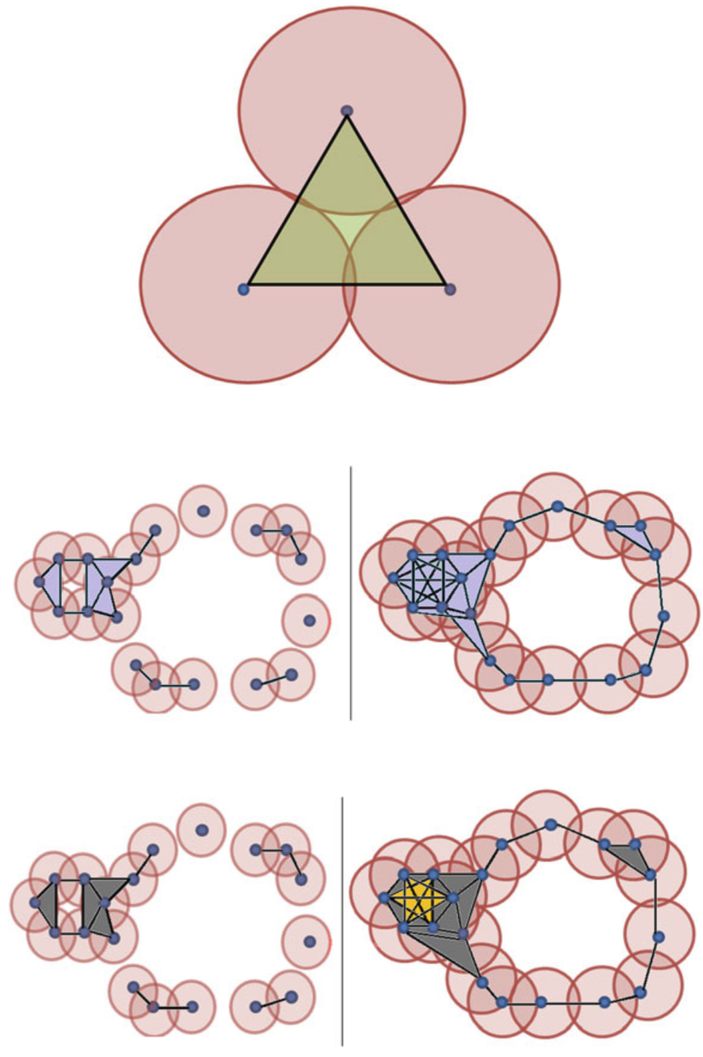
Figure 8.
Vietrois-Rips Vs Alpha Filtration, Vietoris-Rips fails to capture non empty intersection[25]
Figure 8.
Vietrois-Rips Vs Alpha Filtration, Vietoris-Rips fails to capture non empty intersection[25]
5.9. Computational Complexity
As outlined in [31], we avoided creating full Delaunay complex and removing simplices which do not come from a Voronoi face, which has a circumscribing circle carrying no near by points. We achieved this by incrementally going over distance matrix/simplex tree based design only including faces satisfying Nerve Theorem (i.e., intersection of balls was not empty). We also used Simplical Set backing ACSets, allowing further exploration related to gluing options involving spaces with curvatures. We exploited empty circum-sphere property, stating 3-simplex tetrahedron belongs to , if and only if its circum-sphere contains no points [34]
5.10. Observations
5.10.1. Vietoris-Rips Does Not Capture Scale Accurately
With each filtration, Vietoris-Rips generate large multi-dimensional simplical complex without accurately capturing structure. At each filtration, we merely get an approximation of the structure of the underlying space.

Table 3.
Vietoris-Rips vs Alpha : Homology information captured with filtration.
| Filtrations | Vietoris-Rips | Alpha |
| 1.5 | h1 = 0 | h1 = 0 |
| 2.5 | h1 = 5 | h1 = 21 |
| 3.5 | h1 = 0 | h1 = 75 |
| 3.9 | h1 = 0 | h1 = 12 |
| 5.0 | h1 = 0 | h1 = 3 |
5.10.2. Vietoris-Rips Grows Exponentially With Points
We need to restrict dimension otherwise our calculations will take hours, preventing us from trying other options. We restricted our explorations to 4 dimensions. We do not keep higher dimensional structures in memory or process them any further after gaining all tetrahedrons.
5.10.3. Reductions Play a Key Role In Reducing Complexity
We did not pre-process data. We broke down addition of higher dimensional simplices into 2 separate steps.
First step added triangles and tetrahedrons into simplex tree, after vertices and edges were added, if we encountered non duplicate structures confirming non empty intersection of Balls in play (3 for triangles and 4 for tetrahedrons) for Alpha Complexes and checking presence of edges under filtration constraint for Vietoris-Rips complex.
Second step performed actual reduction of non adding multiple zero cycle elements over and over [35]. We did not collapse edges etc.. as on 28 core machine with 56 GB memory, we could run through all 5 filtrations in less than 20 minutes, largest taking about 10 minutes for filtration ball radius of 5.0.
5.11. Implementation
We used Simplex Tree to organize our simplicials such that any node and all its edges can be looked at by only going one level down on a simplex tree.
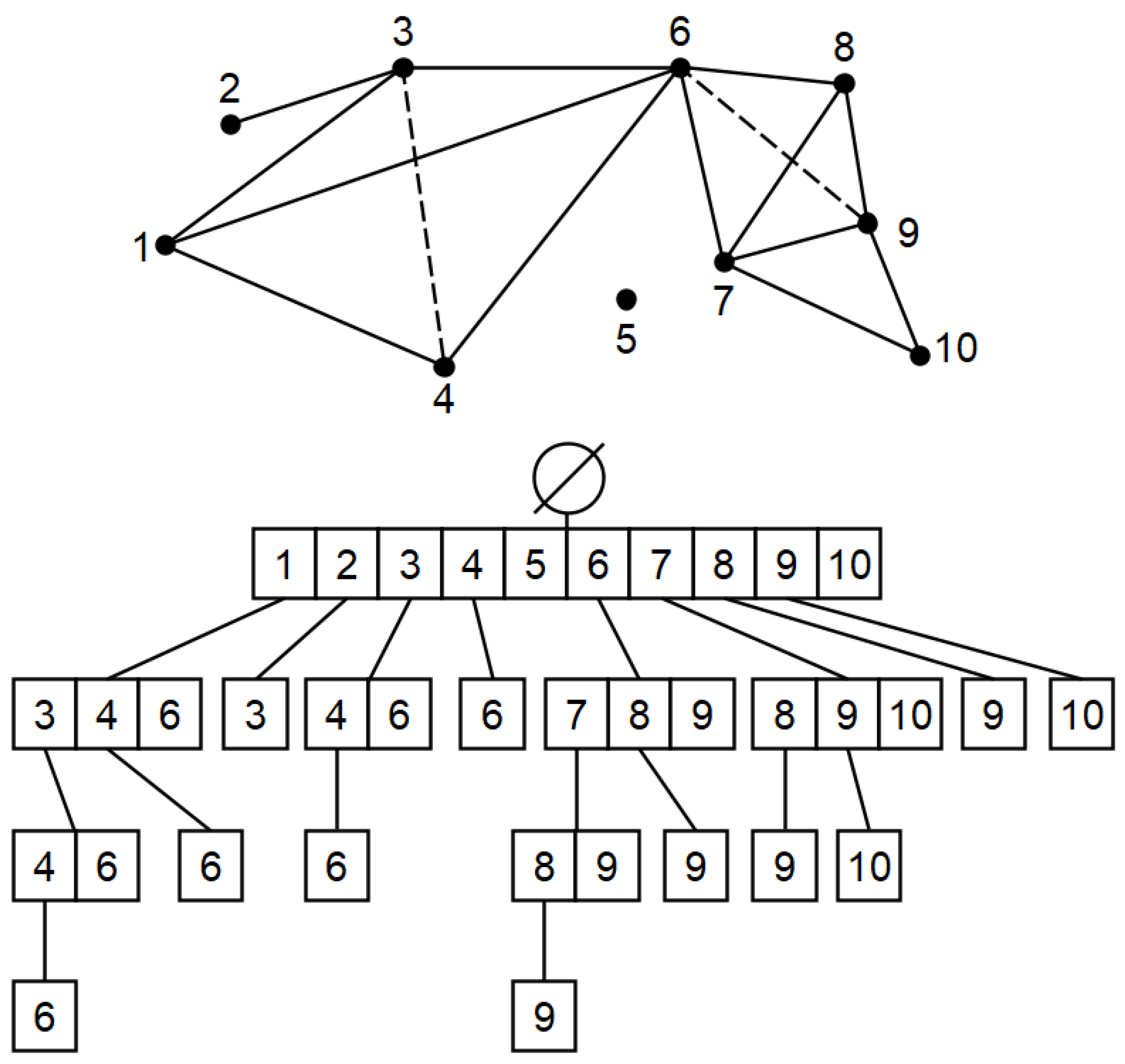
Figure 9.
Simplex Tree, Source : Wikipedia.
We use 2 other data structures, one for managing gluing (process of connecting topological structures) using Simplicial Sets build on top of C-Sets, and the other to manage reduction of 3 and 4 dimensional structures coming in to reduction algorithm in top level driver file with first three nodes forming a tuple as key. This for Vietoris-Rips, prevents repeated duplication of 0 cycles.
Using the same structure with tuple as key, We insert observed triangles as order in which traingles and tetrahedrons arrive changes significantly for Alpha complexes. Knowing what has already been seen, helps us organize for correct orientation, resulting in proper calculation of homologies.
These steps allow for independent implementation and experimentation of various reduction algorithms. We recommend using Rank function from LinearAlgebra packages over other methods (RowEchelon.jl, SmithNormalForm.jl etc..) due to better numerical stability.
5.11.1. Computation over Z2
Using Nemo, one can create a ResidueRing and then perform all rank computations using LinearAlgebra.rank over Z2 disregarding orientations, however we see biggest gains in performance due to reduction/proper handling of orientations by not even injecting them in to matrix. For example, it is not uncommon to see 136126 triangles and 8794 tetrahedrons creating 1197 million element matrix. This can be easily reduced by ignoring insertion of alternating structures over and over.
We leave Z2 based computations as a fall back method if orientations tracking go wrong.
6. Results
6.1. Working Transformer Model
We started out with bert-base-uncased and trained it on our dataset by dividing data in 3 sets; 14000 for training, 3000 for validation and finally we randomly picket 300 sentences out of unseen 3000 test set to verify model correctness. As before we can do any TDA analysis of transformer, transformer has to work. vinay_bert_classifier.py file has lines 254 to 277 commented out, which can be used to retrain model. We used same file for extracting embeddings, sentence_transformer experimentation and avaeraging of embeddings for entire paragraph experiments so feel free to utilize that code as well. In our experience, sentence_transformer (SBERT) pooling layers became completely corrupt after training sentence_transformer could not find enough similarities anywhere, thus declaring all AI/Human generated texts with 86 percent probability as AI text.
If you just want to try some sentences from your favorite Generative AI model (Deepseek, GPT, Grok-3), see vinay_bert_bertgen_11_cls.py Lines 74 to 88, see Line 290 for model loading code. Our transformer model can be used directly from following google drive. Just copy it to your local drive and run python script.
We are adding "[CLS] ", start of paragraph token at Lines 305 to 311. This is not needed for Grok-3, GPT4.x or Deepseek. If you have your own model, you may want to ensure that such token exists at start of your generated paragraph.
Files vinay_bert_bertgen_[1..12]_cls.py are also used to generate 768 byte embeddings of "[CLS ]" token from layers 1 to 12 (in pickle format line 398-401) for any random set of paragraphs using DATA_COUNT and Offset (Line 352). LAYER selects transformer layer and hidden_states[LAYER][0][0] picks "[CLS] " token BERT vector. See line 331 for shape of hidden_states.
This way we do not build any bias in topological data analysis and keep all Alpha Complex/ Vietoris-Rips based analysis, agnostic to any ordering of sentences present in dataset.
For testing model for any unseen, AI or Human written text, see lines 287 to 346 of vinay_bert_bertgen_11_cls.py. One can create BERT vectors from these unseen non dataset sentences and dump them for any transformer layer using code at lines 350 to 401, just by changing line 354 that passes text from dataset to tokenizer.
Use tar xvzf to extract models.
To just run prediction for text and do cosine similarity calculations using bert-base-uncased or just to reproduce sentence_transformer results, see vinay_bert_classifier.py while not using lines 340 to 374 as xgboost did not pick up sentence_transformer embeddings correctly. This file only has examples from dataset.
BERT Model : https://drive.google.com/drive/u/1/folders/1PEH1rTYDwVQgrilJfWoldg4DiBEn85j3 Use BERT model for Human/Ai text classification.
SBERT Model : https://drive.google.com/drive/u/1/folders/1PEH1rTYDwVQgrilJfWoldg4DiBEn85j3
SBERT declared every sentence as AI generated text with 87 percent confidence due to its pooling layer corruption as it could not learn interplay of context among words from AI text and Human generated texts.
Figure 10.
1-3 Layers of bert-base-uncased Vietoris-Rips vs Alpha Complex.
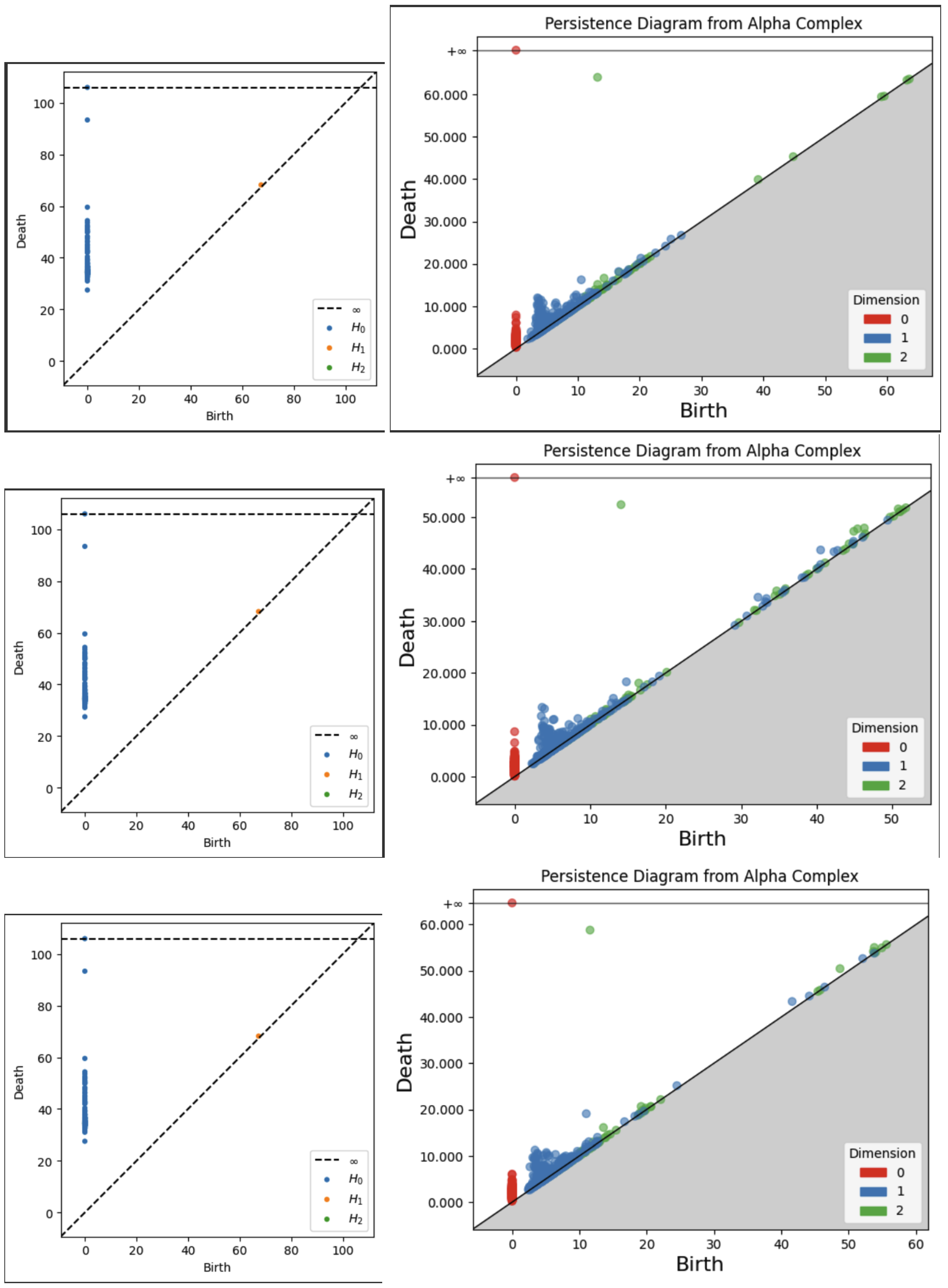
Figure 11.
3-6 Layers of bert-base-uncased Vietoris-Rips vs Alpha Complex.
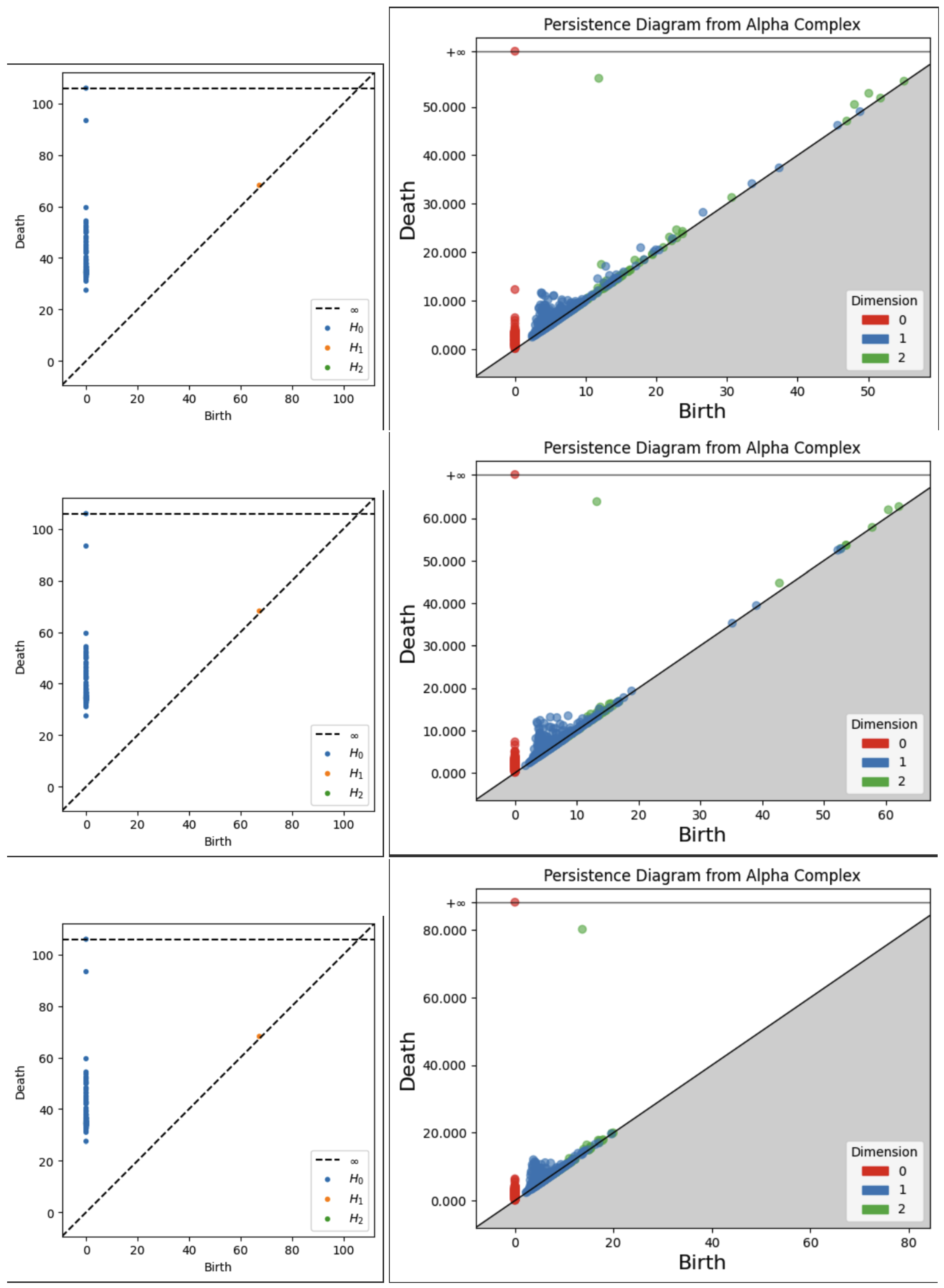
Figure 12.
6-9 Layers of bert-base-uncased Vietoris-Rips vs Alpha Complex.
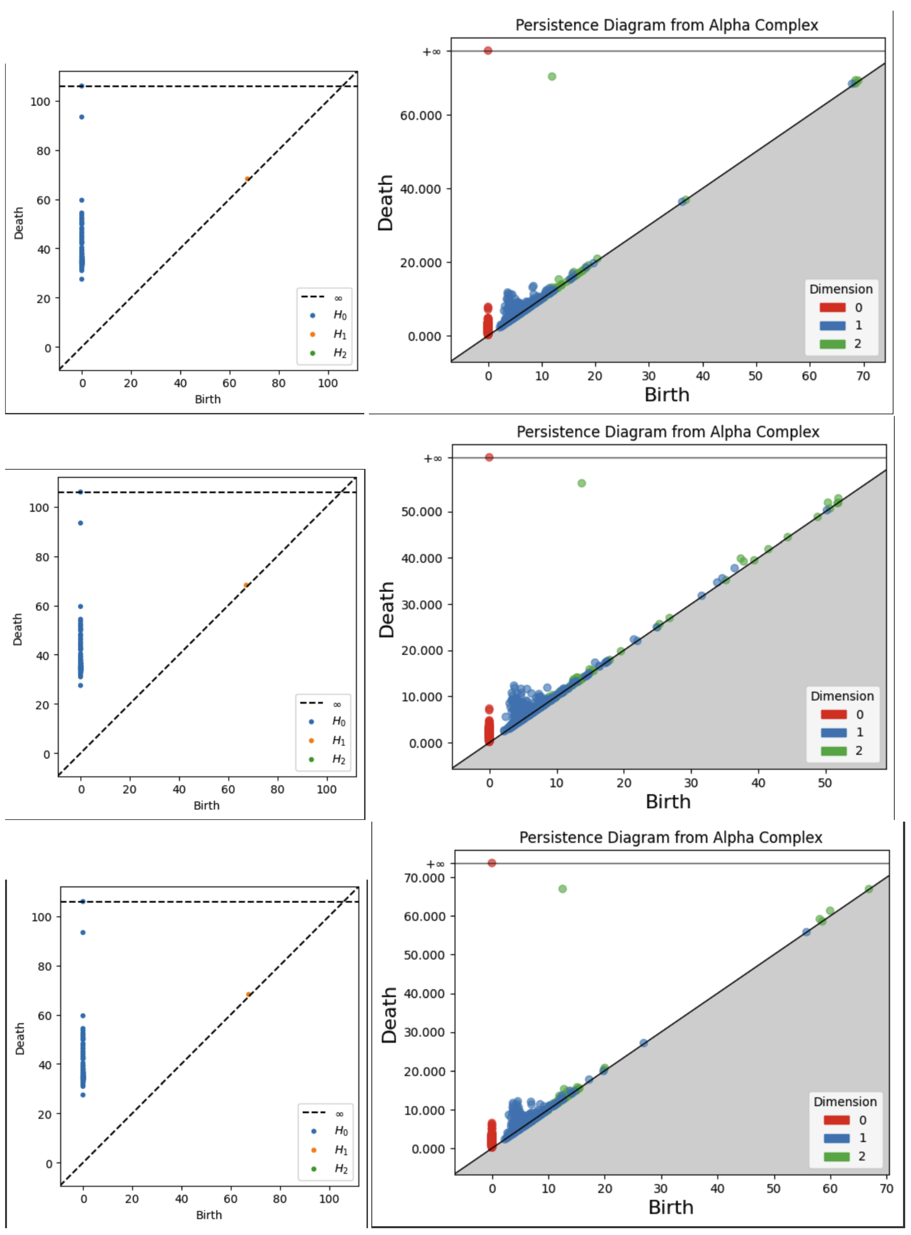
Figure 13.
9-12 Layers of bert-base-uncased Vietoris-Rips vs Alpha Complex.

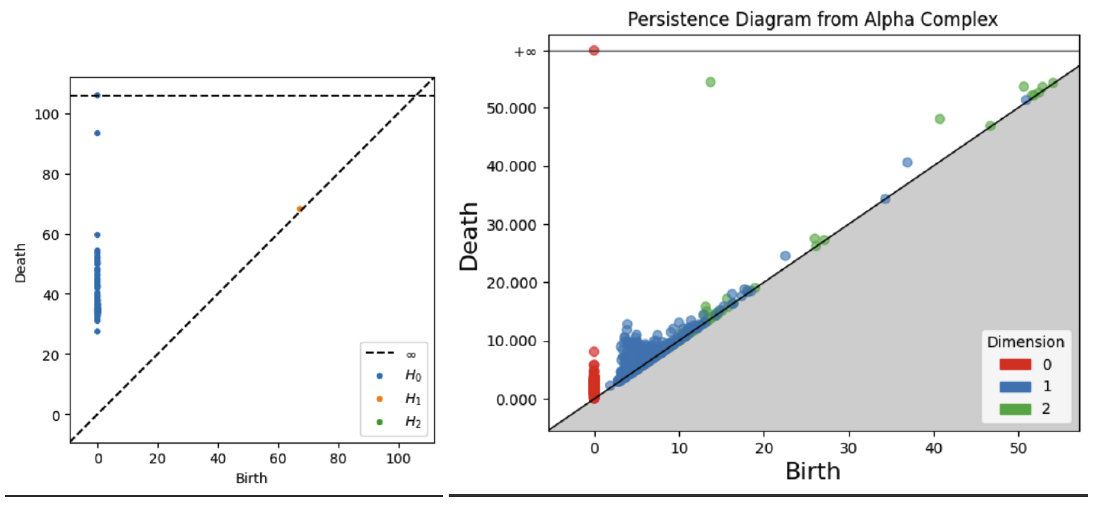
Figure 14.
Classification Head of bert-base-uncased Vietoris-Rips vs Alpha Complex.
7. Conclusions
Vietoris Rips is not a suitable tool for analyzing transformer topological homological properties.
Appendix A. Embeddings
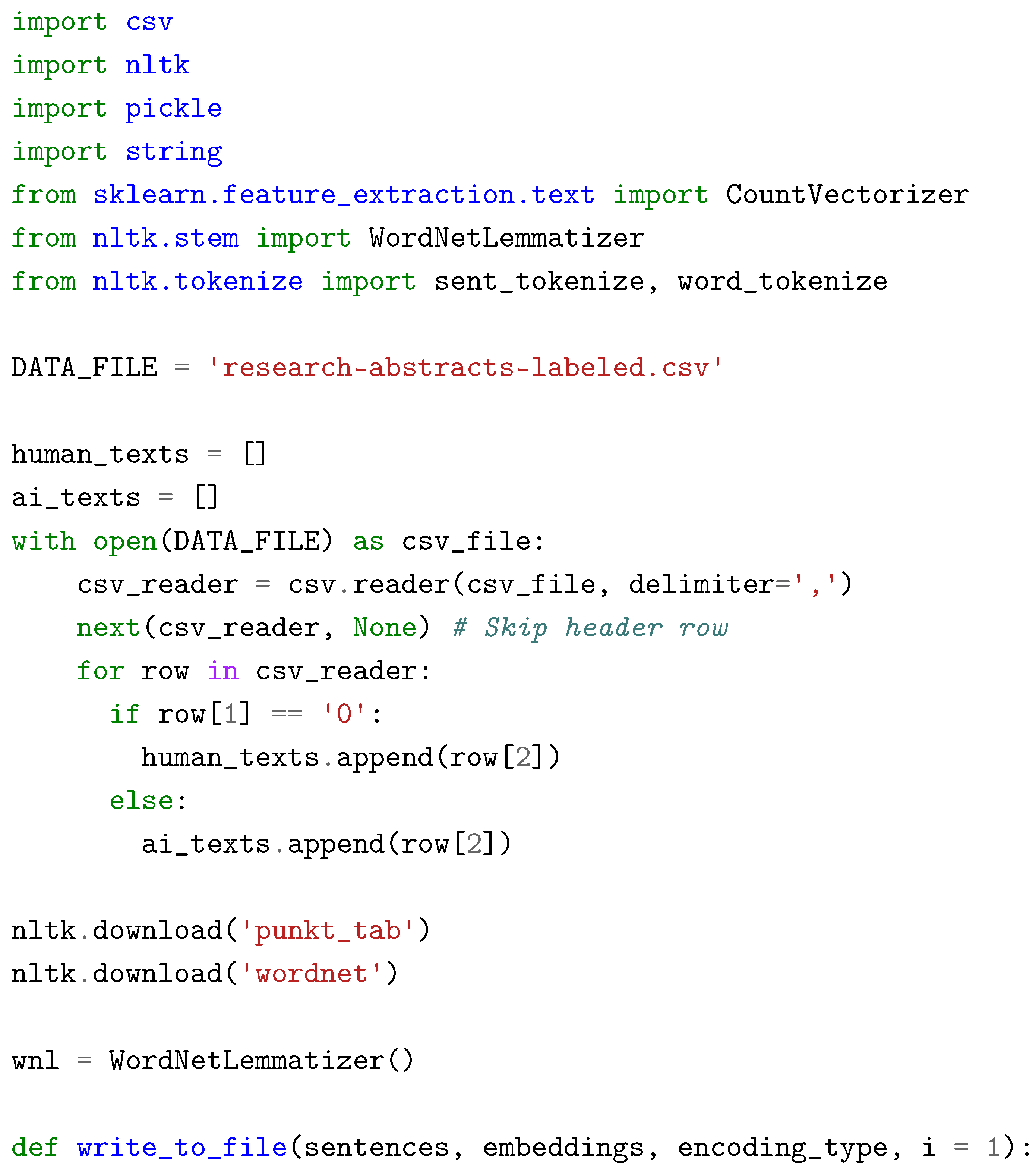
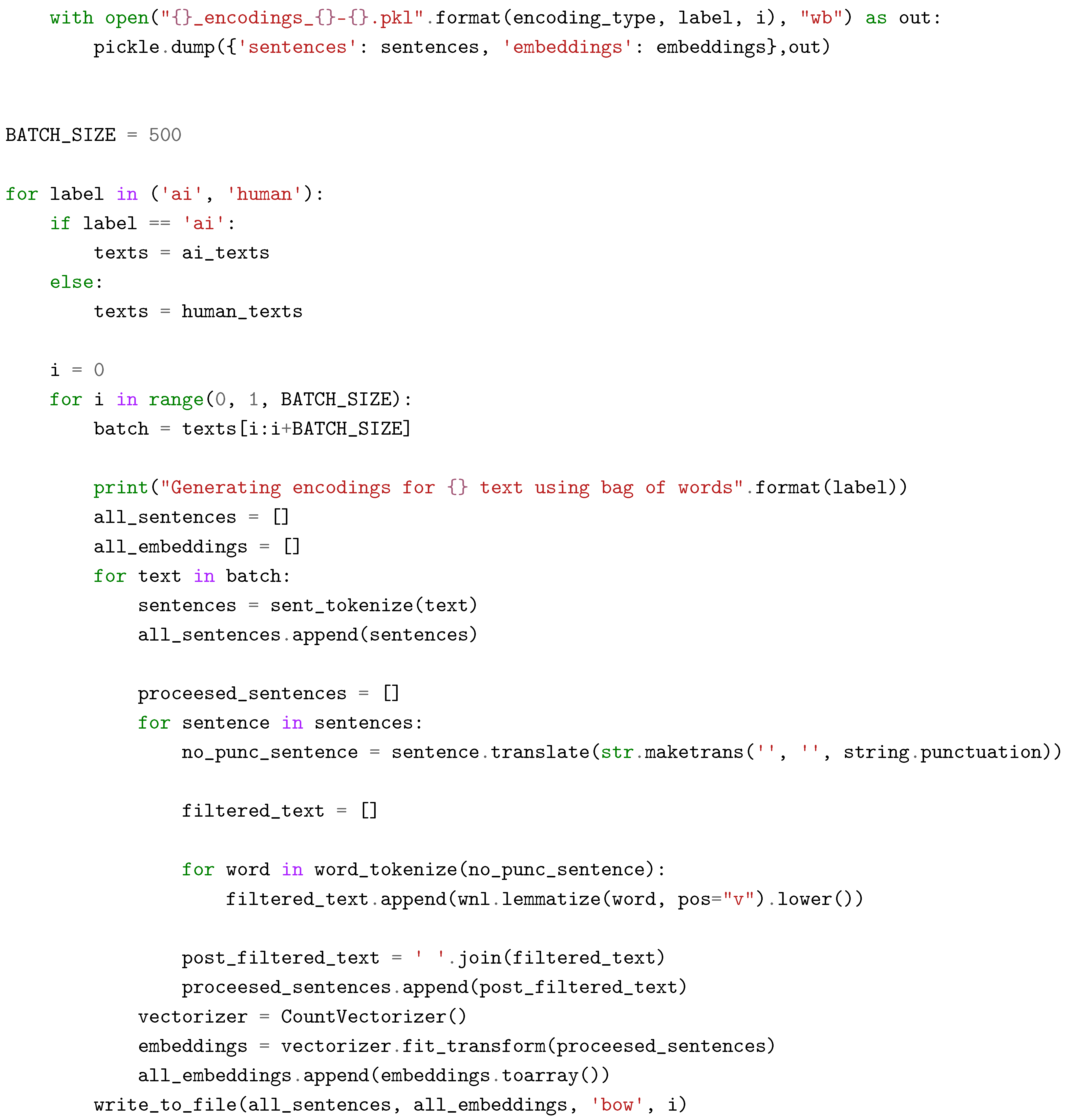
Appendix A.1. Bag Of Words
Python code for generating BoW embeddings for the abstracts data
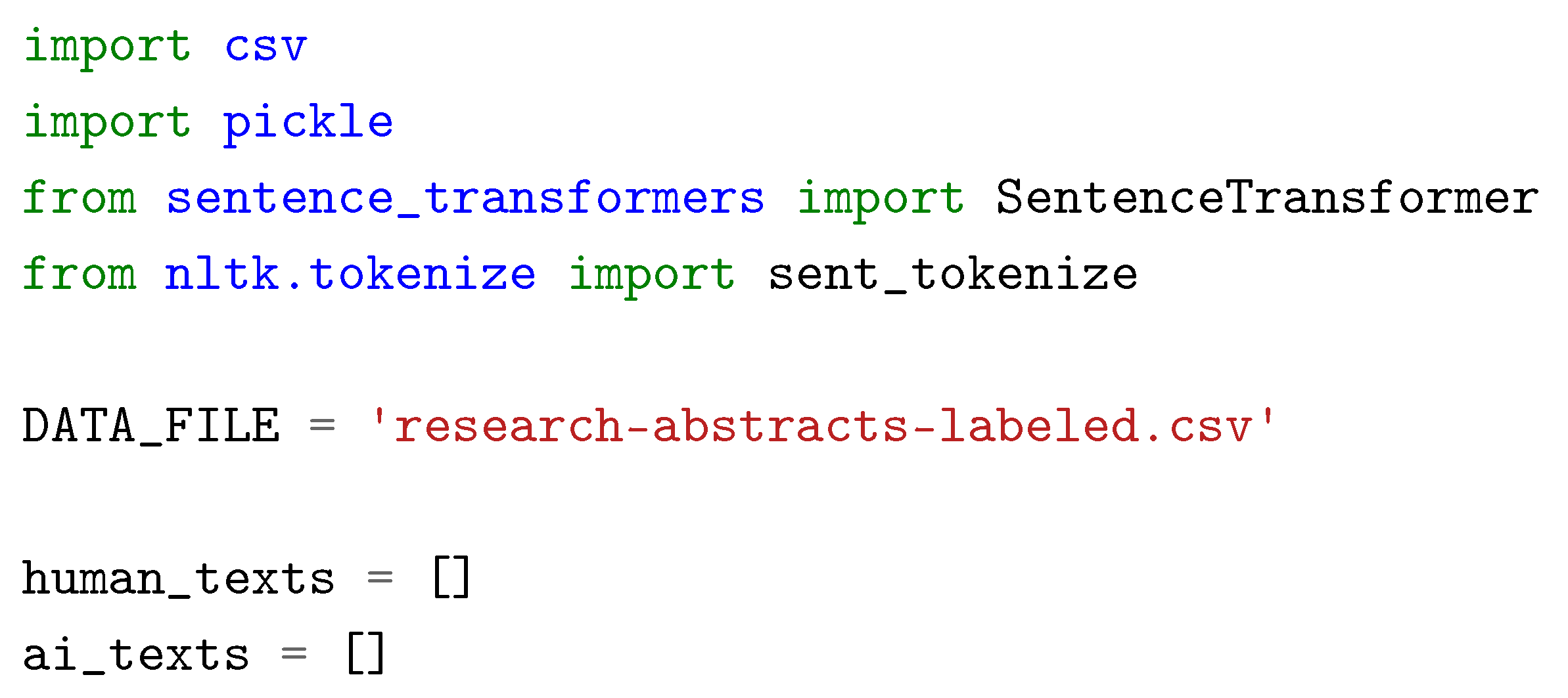
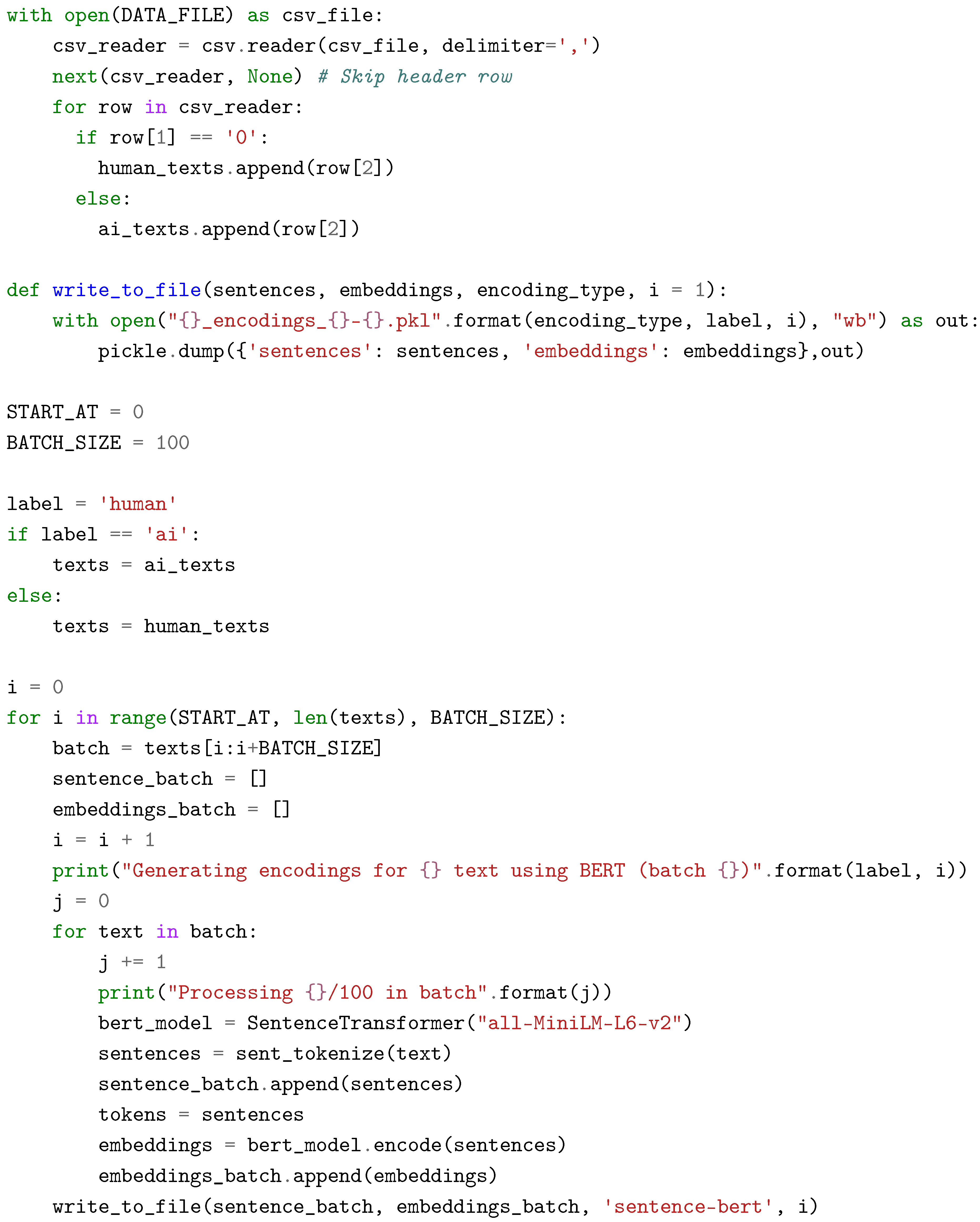
Appendix A.2. SBERT
Python code for generating SBERT embeddings for the abstracts data
Appendix B. Persistence for Vietoris-Rips
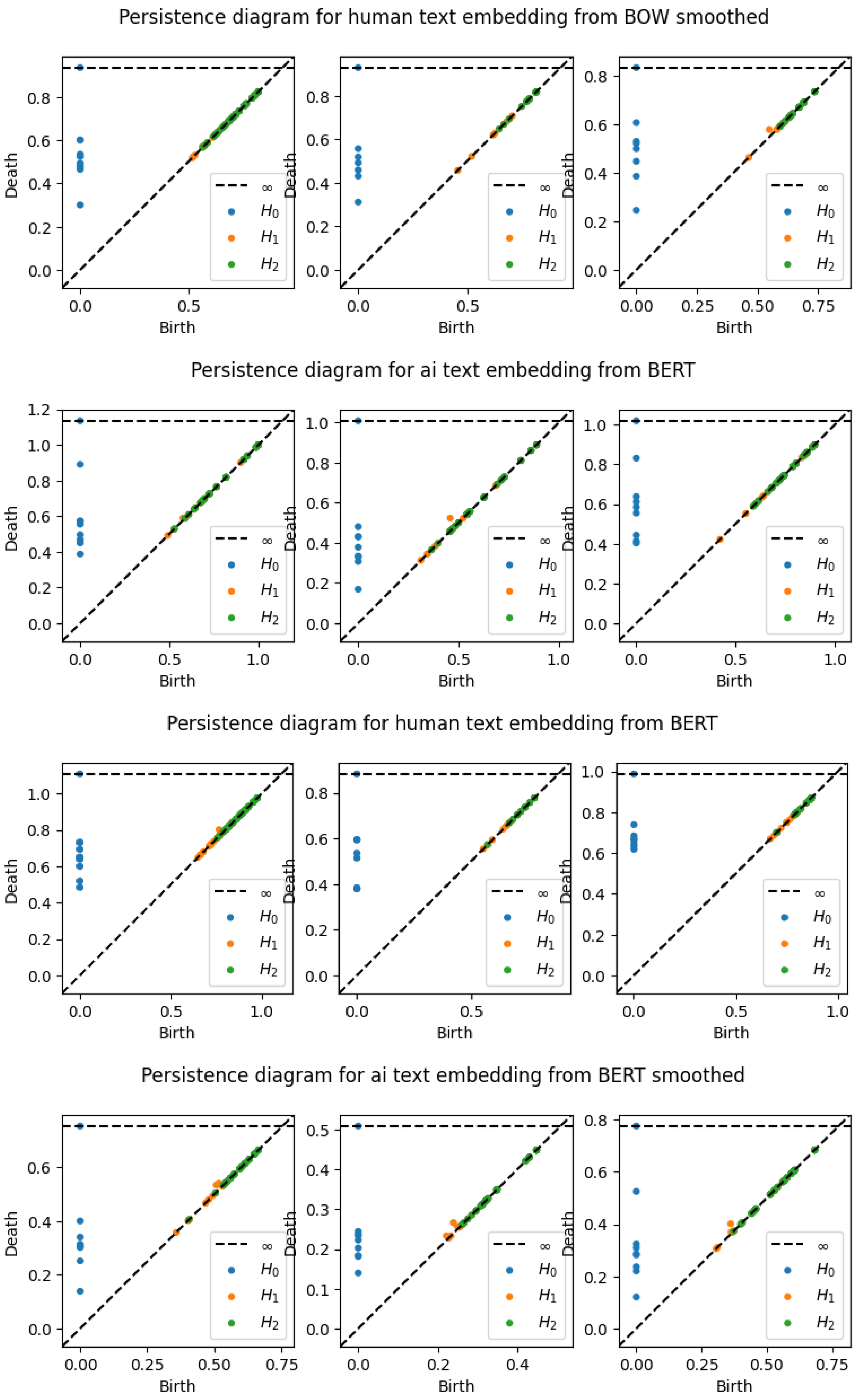
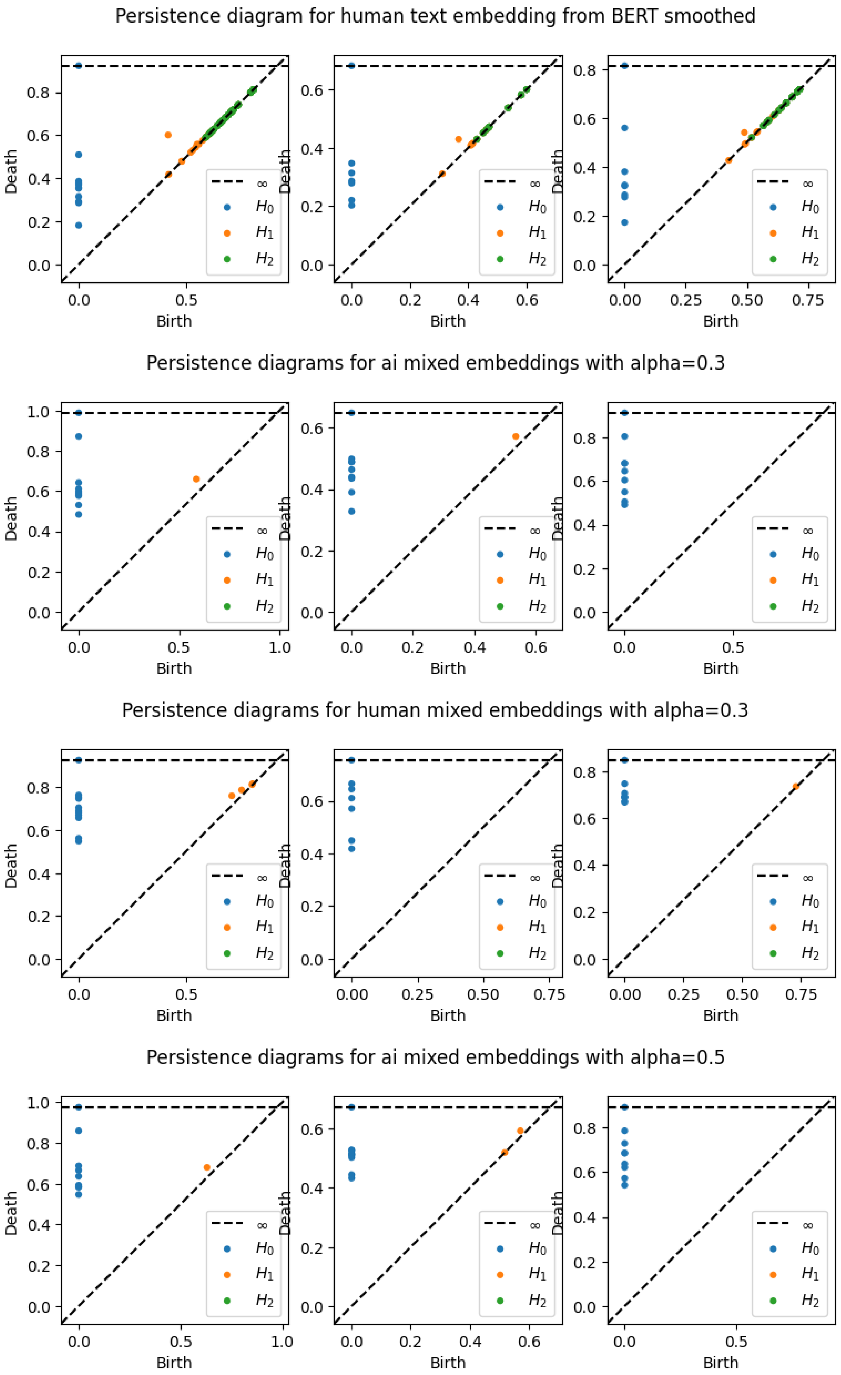
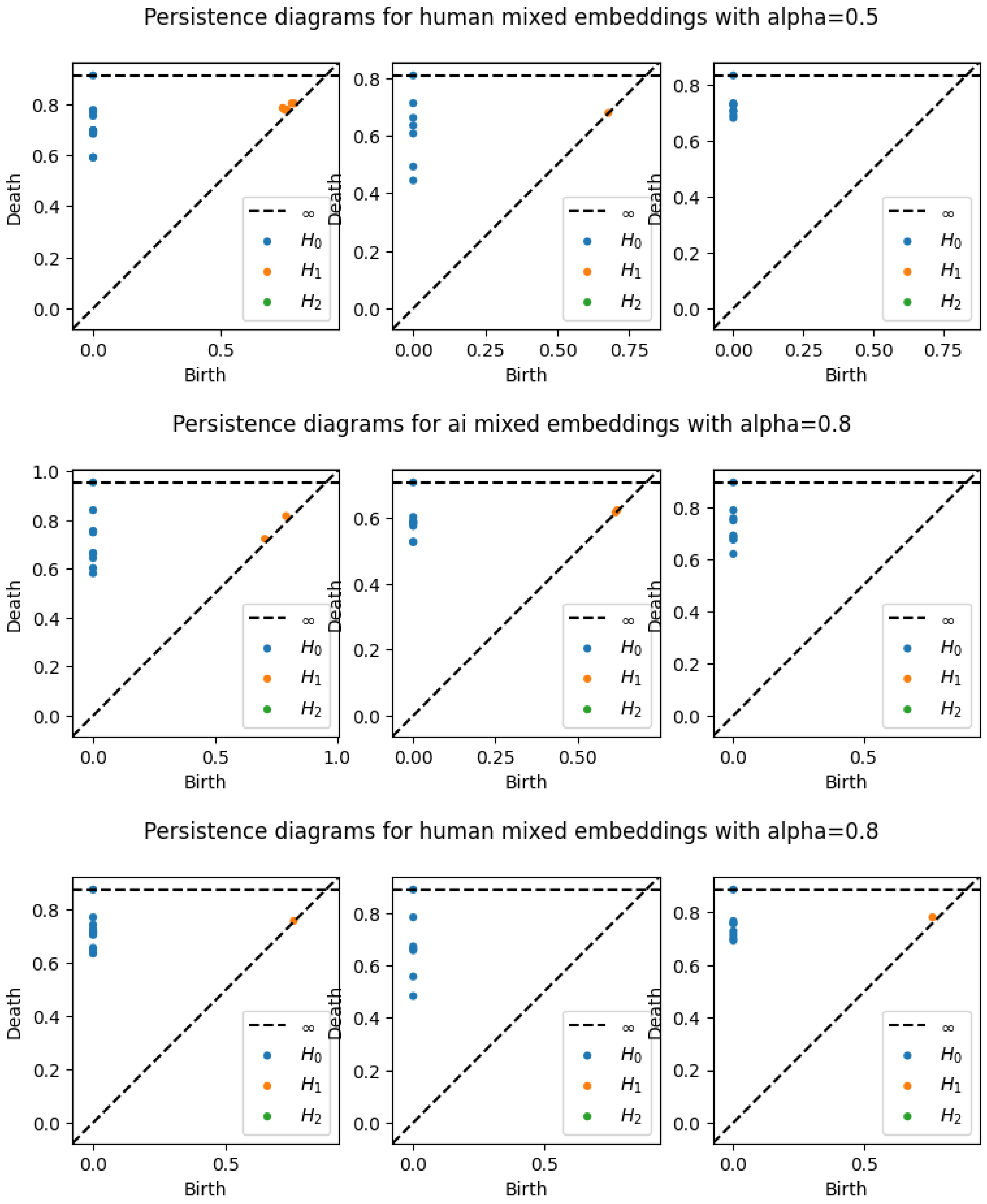
Appendix B.1. Persistence Diagrams
A sample of the persistence diagrams for the first 3 abstracts across embedding types, smoothing, and alpha values for the compose metric. Note that ’BERT’ represents SBERT embeddings, and "mixed" embeddings indicates use of the composite metric.

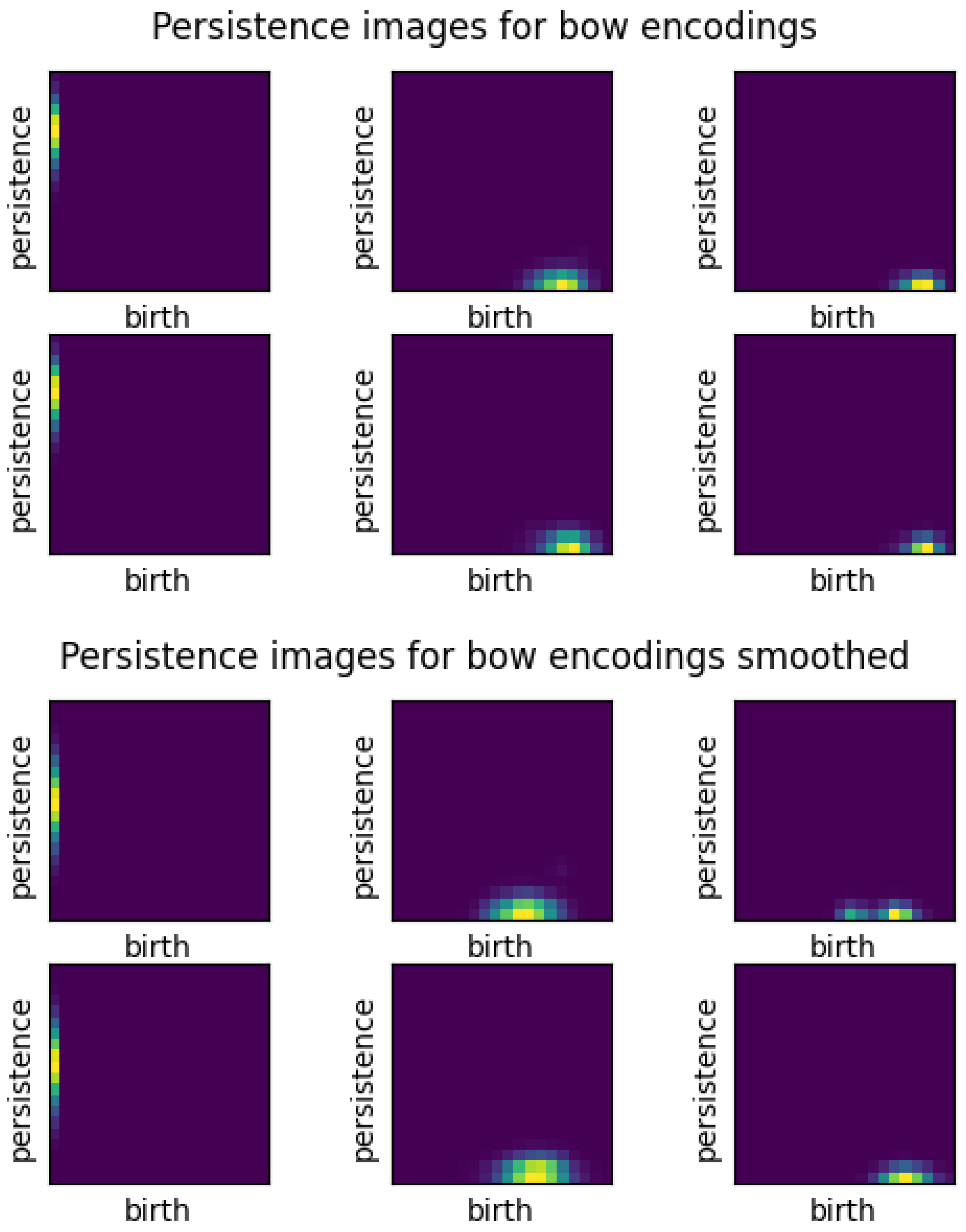
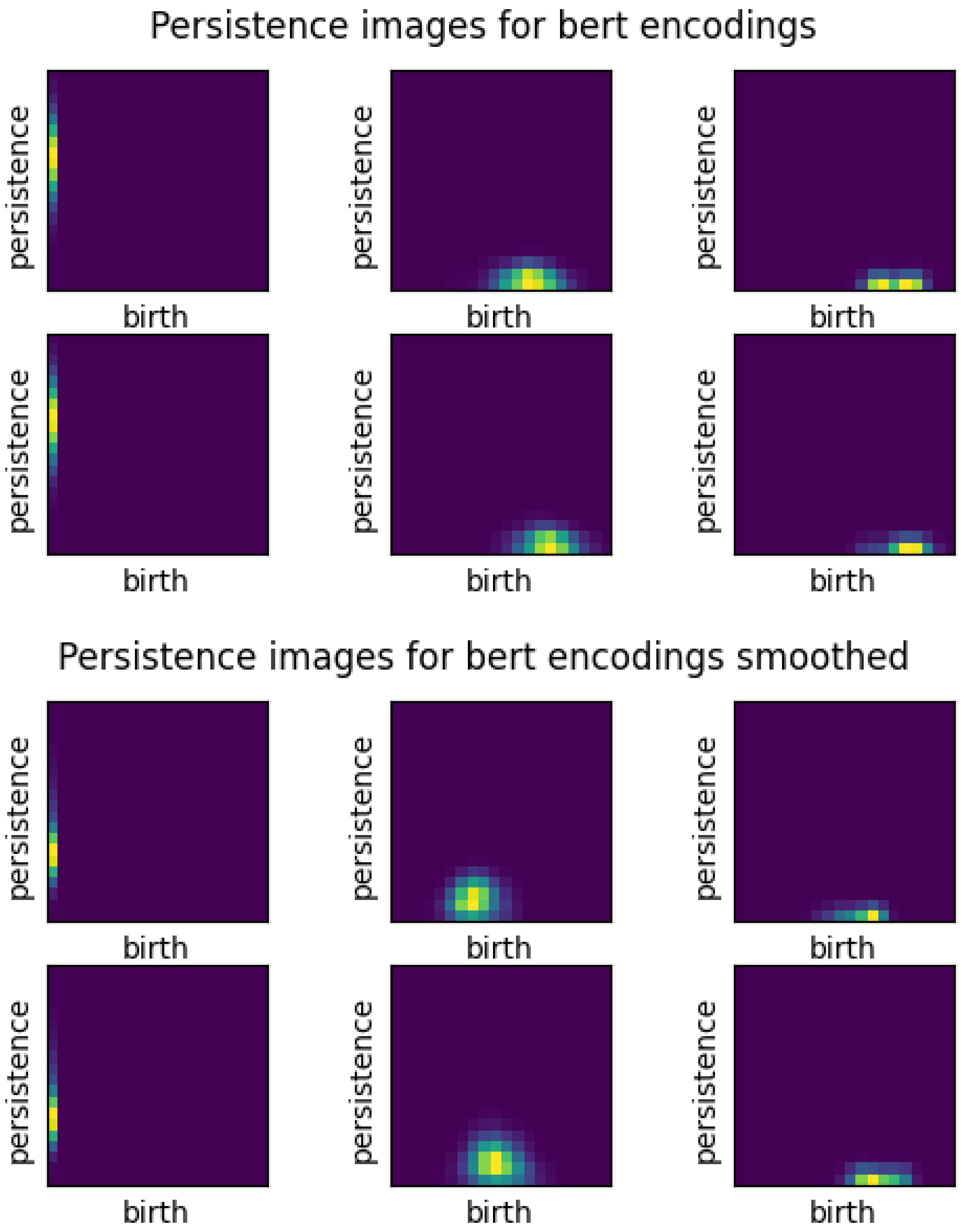
Appendix B.2. Persistence Images
The averaged persistence images across embedding types, smoothing, and alpha values for the compose metric for 1000 abstracts. For each image, the top row represents the image for the group of AI text and the bottom row is human text. The first column shows H0, the second H1, and the last column is H2. Again, ’BERT’ represents SBERT embeddings, and "mixed" embeddings indicates use of the composite metric.
References
- Gerlich, M. AI Tools in Society: Impacts on Cognitive Offloading and the Future of Critical Thinking. Societies 2025, 15. [Google Scholar] [CrossRef]
- Bataineh, A.A.; Sickler, R.; Kurcz, K.; Pedersen, K. AI-Generated vs. Human Text: Introducing a New Dataset for Benchmarking and Analysis. IEEE Transactions on Artificial Intelligence 2025, pp. 1–11. [CrossRef]
- Ma, Y.; Liu, J.; Yi, F.; Cheng, Q.; Huang, Y.; Lu, W.; Liu, X. AI vs. Human – Differentiation Analysis of Scientific Content Generation, 2023, [arXiv:cs.CL/2301.10416].
- Draganov, O.; Skiena, S. The Shape of Word Embeddings: Quantifying Non-Isometry with Topological Data Analysis. In Proceedings of the Findings of the Association for Computational Linguistics: EMNLP 2024. Association for Computational Linguistics; 2024; pp. 12080–12099. [Google Scholar] [CrossRef]
- Zhu, X. Persistent homology: An introduction and a new text representation for natural language processing. 08 2013, pp. 1953–1959.
- Uchendu, A.; Le, T. Unveiling Topological Structures in Text: A Comprehensive Survey of Topological Data Analysis Applications in NLP, 2024, [arXiv:cs.CL/2411.10298].
- Solberg. Text Classification via Topological Data Analysis. Master’s thesis, 2023.
- Tymochko, S.; Chaput, J.; Doster, T.; Purvine, E.; Warley, J.; Emerson, T. Con Connections: Detecting Fraud from Abstracts using Topological Data Analysis. In Proceedings of the 2021 20th IEEE International Conference on Machine Learning and Applications (ICMLA), 2021, pp. 403–408. [CrossRef]
- Nicolai Thorer Sivesind, A. Human-vs-Machine. https://huggingface.co/datasets/NicolaiSivesind/human-vs-machine, 2023.
- Fröhling, L.; Zubiaga, A. Feature-based detection of automated language models: tackling GPT-2, GPT-3 and Grover. PeerJ Computer Science 2021, 7, e443. [Google Scholar] [CrossRef] [PubMed]
- Devlin, J.; Chang, M.W.; Lee, K.; Toutanova, K. BERT: Pre-training of Deep Bidirectional Transformers for Language Understanding. In Proceedings of the Proceedings of the 2019 Conference of the North American Chapter of the Association for Computational Linguistics: Human Language Technologies, Volume 1 (Long and Short Papers); Burstein, J.; Doran, C.; Solorio, T., Eds., Minneapolis, Minnesota, 2019; pp. 4171–4186. [CrossRef]
- Reimers, N.; Gurevych, I. Sentence-BERT: Sentence Embeddings using Siamese BERT-Networks, 2019, [arXiv:cs.CL/1908.10084].
- sentence-transformers/all-MiniLM-L6-v2. https://huggingface.co/sentence-transformers/all-MiniLM-L6-v2.
- Strehl, A.; Ghosh, J.; Mooney, R. Impact of Similarity Measures on Web-page Clustering. In Proceedings of the Proceedings of the Workshop on Artificial Intelligence for Web Search (AAAI 2000). AAAI Press, 2000.
- Deisenroth, M.P.; Faisal, A.A.; Ong, C.S. Mathematics for Machine Learning; Cambridge University Press, 2020.
- Gholizadeh, S.; Seyeditabari, A.; Zadrozny, W. A Novel Method of Extracting Topological Features from Word Embeddings. CoRR 2020, abs/2003.13074, [2003.13074].
- Zomorodian, A.J. Spaces and Filtrations. In Topology for Computing; Cambridge Monographs on Applied and Computational Mathematics, Cambridge University Press, 2005; p. 13–40.
- Edelsbrunner, H.; Harer, J. Computational topology: An introduction; American Mathematical Society, 2010.
- Tralie, C.; Saul, N.; Bar-On, R. Ripser.py: A Lean Persistent Homology Library for Python. The Journal of Open Source Software 2018, 3, 925. [Google Scholar] [CrossRef]
- Cohen-Steiner, Edelsbrunner, H. Stability of Persistence Diagrams. Discrete & Computational Geometry 2006, 37, 103–120. [Google Scholar] [CrossRef]
- Adams, e.a. Persistence Images: A Stable Vector Representation of Persistent Homology. Journal of Machine Learning Research 2017, 18, 1–35. [Google Scholar]
- Bethany, M.; Wherry, B.; Bethany, E.; Vishwamitra, N.; Rios, A.; Najafirad, P. Deciphering Textual Authenticity: A Generalized Strategy through the Lens of Large Language Semantics for Detecting Human vs. Machine-Generated Text. In Proceedings of the 33rd USENIX Security Symposium (USENIX Security 24), Philadelphia, PA, 2024; pp. 5805–5822.
- Stephen Fitz, Peter Romero, J.J.S. Hidden Holes topological aspects of language models, 2024, [arXiv:cs.CL/2406.05798v1].
- Luis Balderas 1, M.L.; Ben´ıtez, J.M. Can persistent homology whiten Transformer-based black-box models? A case study on BERT compression, 2023, [arXiv:cs.LG/2312.10702].
- Nanda, V.; Sazdanovi´c, R. Simplicial Models and Topological Inference in Biological Systems. Discrete and Topological Models in Molecular Biology, Springer-Verlag 2014. [CrossRef]
- Lundberg, S.; Lee, S.I. A Unified Approach to Interpreting Model Predictions, 2017, [arXiv:cs.AI/1705.07874].
- Shumailov, I.; Shumaylov, Z.; Zhao, Y.; Gal, Y.; Papernot, N.; Anderson, R. The Curse of Recursion: Training on Generated Data Makes Models Forget, 2024, [arXiv:cs.LG/2305.17493].
- Liu, Z.; Jin, W.; Mu, Y. Subspace embedding for classification. Neural Computing and Applications 2022, 34, 18407–18420. [Google Scholar] [CrossRef]
- Clarkson, K.L.; Woodruff, D.P. Low Rank Approximation and Regression in Input Sparsity Time, 2013, [arXiv:cs.DS/1207.6365].
- Bauer, U. Ripser: efficient computation of Vietoris–Rips persistence barcodes. Journal of Applied and Computational Topology 2021, 5, 391–423. [Google Scholar] [CrossRef]
- Erik Carlsson, J.C. Computing the alpha complex using dual active set quadratic programming. Nature Sci Rep 2024, 14. [Google Scholar] [CrossRef] [PubMed]
- Talha Bin Masood a, Tathagata Ray b, V.N.c. Parallel computation of alpha complexes for biomolecules. Elsevier Science Direct 2020. [CrossRef]
- Ulrich Bauer a, Michael Kerber b, F.R.a.A.R.a. A unified view on the functorial nerve theorem and its variations. Expositiones Mathematicae 2023, 41. [CrossRef]
- Hurtado, F., N.M..U.J. Flipping edges in triangulations. In Proceedings of the 12th Annual Symposium on Computational Geometry 1996. https://doi.org/https://dl.acm.org/doi/pdf/10.1145/237218.237367.
- Bauer, U. Ripser: efficient computation of Vietoris-Rips persistence barcodes. arXiv:1908.02518 2019. [CrossRef]
Figure 1.
Example flow for calculating distance from a set of sentences. In this example, Bag of Words is depicted.
Figure 1.
Example flow for calculating distance from a set of sentences. In this example, Bag of Words is depicted.
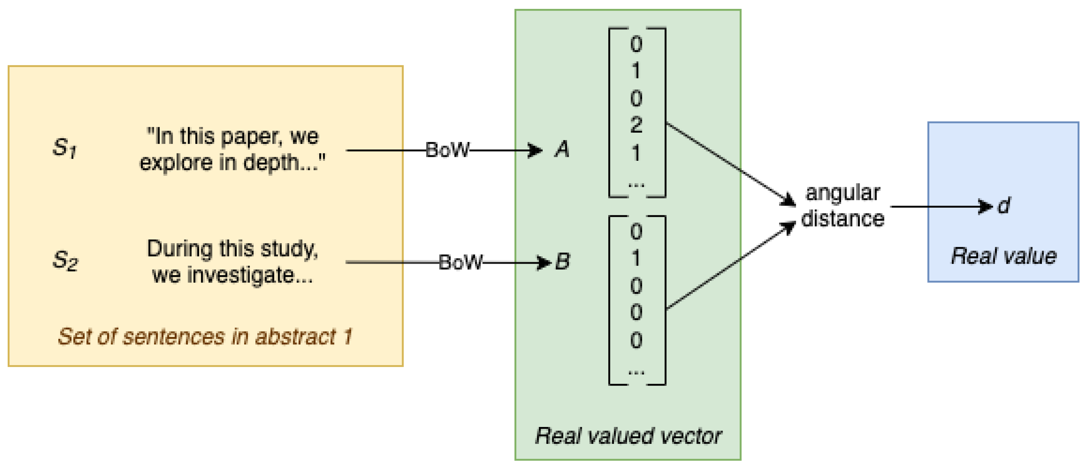
Figure 2.
Example flow for calculating the composite distance from a set of sentences.
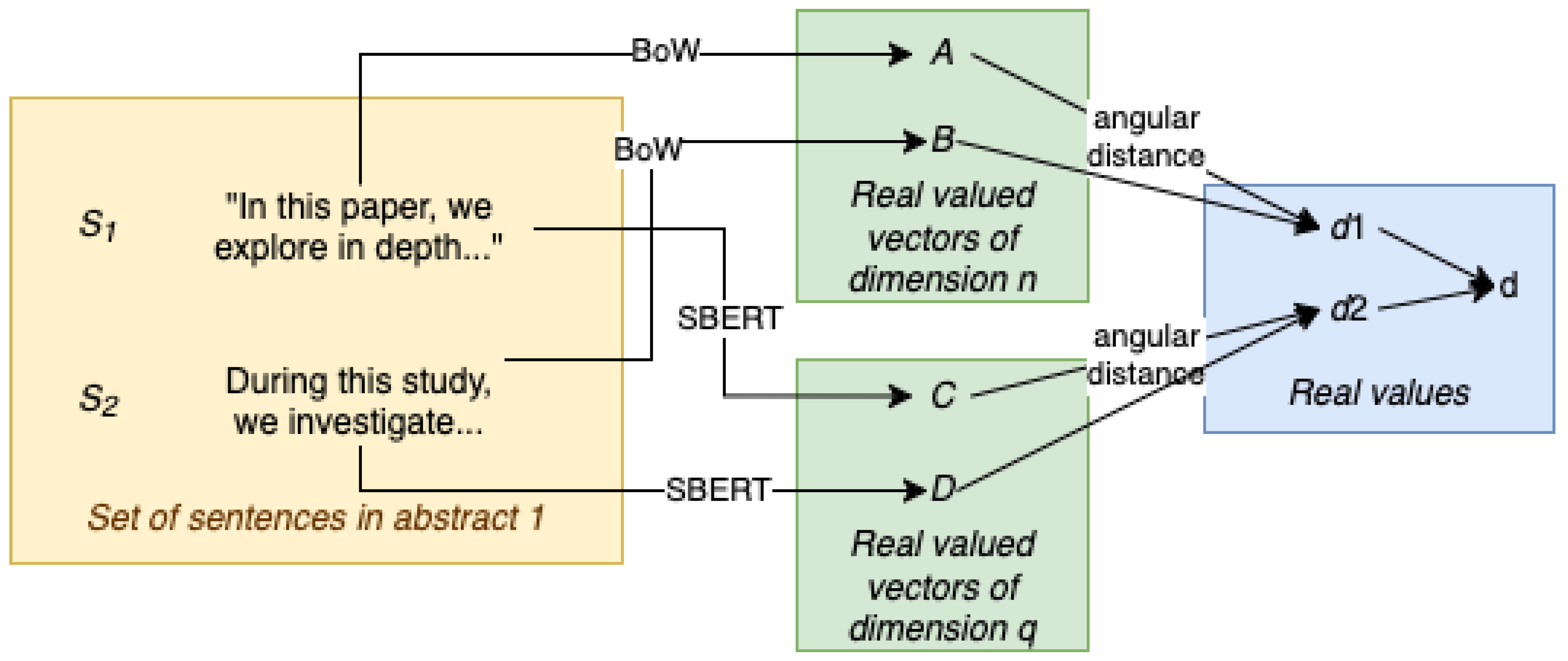
Figure 3.
Distance histograms. The top histograms are from AI-generated abstracts, and the bottom histograms are from human-generated abstracts. All cases use SBERT embeddings and the angular distance metric.
Figure 3.
Distance histograms. The top histograms are from AI-generated abstracts, and the bottom histograms are from human-generated abstracts. All cases use SBERT embeddings and the angular distance metric.
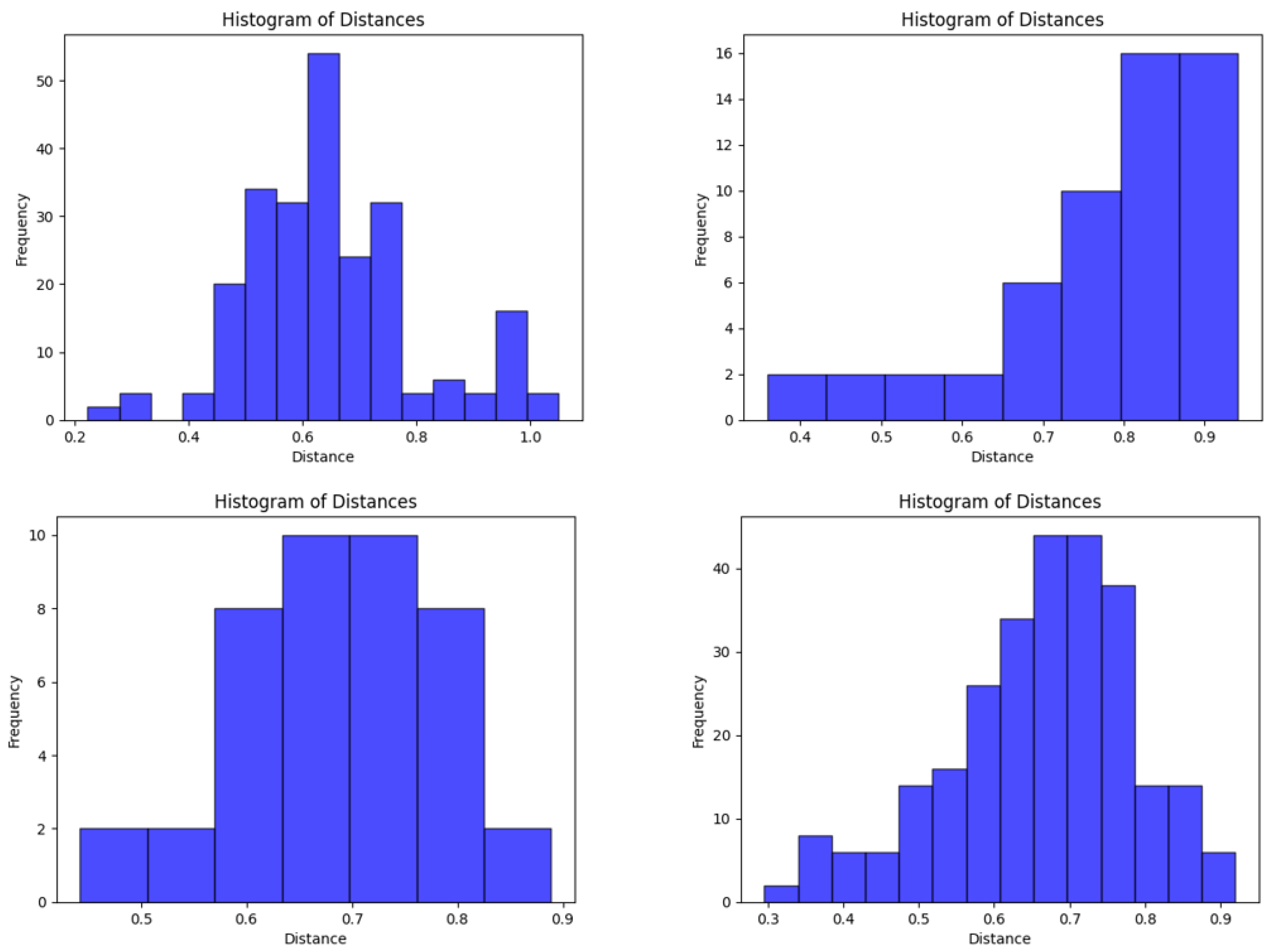
Figure 4.
Two pairs of a persistence diagram with the corresponding H1 persistence image. Taken from two human-written abstracts using smoothed Sentence BERT embedding and angular distance metric.
Figure 4.
Two pairs of a persistence diagram with the corresponding H1 persistence image. Taken from two human-written abstracts using smoothed Sentence BERT embedding and angular distance metric.
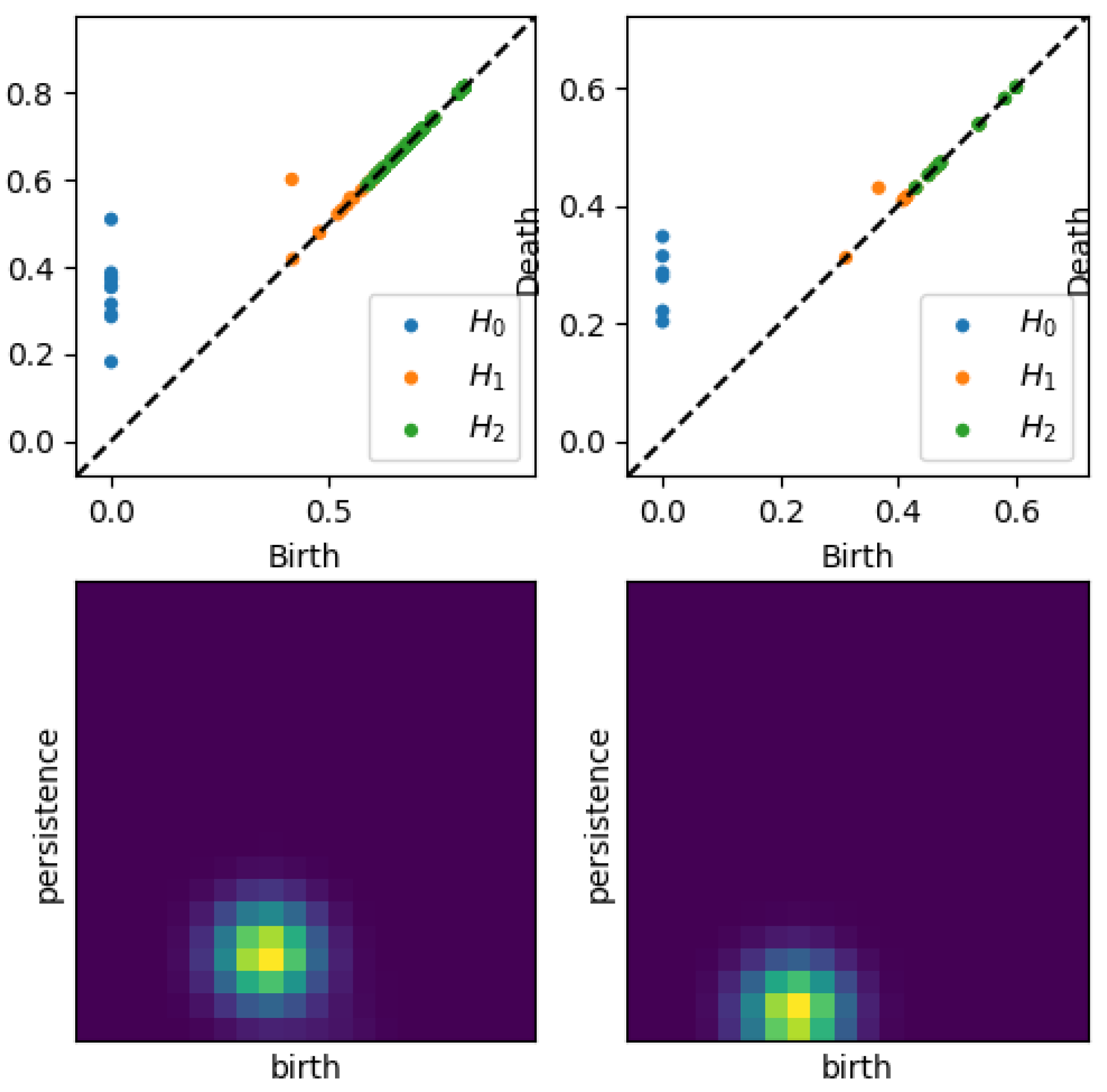
Figure 7.
Two H1 persistence images from different classes. These shown an offset in the center of the “hot” areas while maintaining some overlap.
Figure 7.
Two H1 persistence images from different classes. These shown an offset in the center of the “hot” areas while maintaining some overlap.
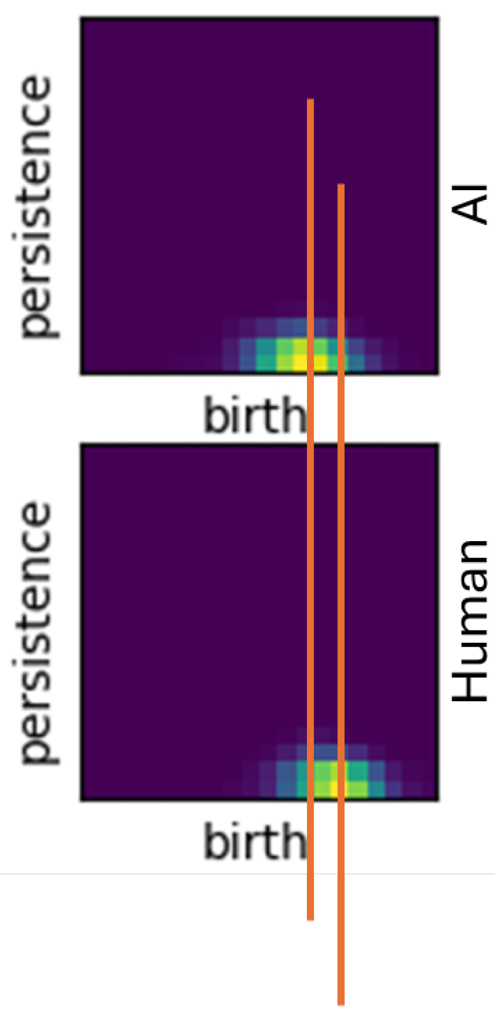
Table 1.
Average number of persistent homologies across any filtration by dimension for AI generated abstracts vs Human using Vietoris-Rips filtrations
Table 1.
Average number of persistent homologies across any filtration by dimension for AI generated abstracts vs Human using Vietoris-Rips filtrations
| Type | AI | Human | AI | Human | AI | Human |
| BoW | 7.861 | 7.555 | 0.869 | 0.883 | 0.043 | 0.057 |
| BoW, smoothed | 7.861 | 7.557 | 0.982 | 0.874 | 0.021 | 0.019 |
| SBERT | 7.86 | 7.555 | 0.814 | 1.086 | 0.032 | 0.053 |
| SBERT, smoothed | 7.861 | 7.558 | 1.102 | 0.992 | 0.016 | 0.032 |
| Composite, | 8.358 | 8.184 | 0.847 | 1.06 | 0.026 | 0.062 |
| Composite, | 8.358 | 8.184 | 0.882 | 1.038 | 0.042 | 0.055 |
| Composite, | 8.358 | 8.184 | 0.961 | 0.976 | 0.05 | 0.059 |
Table 2.
Classification scores for separating AI written abstracts from human written ones when using Vietoris-Rips filtration over 800 training cases and 200 test cases. Dimension high scores are bolded.
Table 2.
Classification scores for separating AI written abstracts from human written ones when using Vietoris-Rips filtration over 800 training cases and 200 test cases. Dimension high scores are bolded.
| H0 | H1 | H2 | ||||
| Type | Linear | Binning | Linear | Binning | Linear | Binning |
| BoW | 0.6497 | 0.6078 | 0.5359 | 0.5359 | 0.5359 | 0.4671 |
| BoW, smoothed | 0.5688 | 0.5494 | 0.5329 | 0.5329 | 0.5359 | 0.4701 |
| SBERT | 0.7814 | 0.7171 | 0.5479 | 0.5659 | 0.5359 | 0.4641 |
| SBERT, smoothed | 0.7485 | 0.6617 | 0.6108 | 0.7036 | 0.5359 | 0.4551 |
| Composite, | 0.705 | 0.665 | 0.5392 | 0.7010 | 0.6875 | 0.5 |
| Composite, | 0.6725 | 0.6725 | 0.5121 | 0.6976 | 0.6111 | 0.7778 |
| Composite, | 0.6213 | 0.5913 | 0.4975 | 0.6281 | 0.5 | 0.6667 |
Disclaimer/Publisher’s Note: The statements, opinions and data contained in all publications are solely those of the individual author(s) and contributor(s) and not of MDPI and/or the editor(s). MDPI and/or the editor(s) disclaim responsibility for any injury to people or property resulting from any ideas, methods, instructions or products referred to in the content. |
© 2025 by the authors. Licensee MDPI, Basel, Switzerland. This article is an open access article distributed under the terms and conditions of the Creative Commons Attribution (CC BY) license (http://creativecommons.org/licenses/by/4.0/).
Copyright: This open access article is published under a Creative Commons CC BY 4.0 license, which permit the free download, distribution, and reuse, provided that the author and preprint are cited in any reuse.


