Submitted:
30 April 2025
Posted:
02 May 2025
You are already at the latest version
Abstract
This article presents a new selective method for identifying a faulty feeder in 6–35 kV electrical distribution networks with isolated neutral configuration during single-phase ground faults (SPGFs) with transient resistance. The method is based on simultaneous comparison of the zero-sequence current (ZSC) angle and magnitude across all outgoing feeders and substation buses. Unlike conventional protection approaches relying solely on current amplitude or direction, the proposed algorithm enhances sensitivity and selectivity by detecting the 180° phase opposition between the faulted feeder's ZSC and the unfaulted feeders’ capacitive ZSC. To implement this strategy, a centralized ground fault protection unit (CGFPU) was developed, capable of real-time feeder status monitoring, fault localization, and differentiated alarm or trip signal generation. Extensive modeling of SPGF processes was conducted in Matlab Simulink, considering transient resistance values ranging from 1 Ω to 10,000 Ω. Results demonstrated the nonlinear behavior of ground fault and capacitive currents relative to the transient resistance, with a notable shift in phasor angles approaching 180° for faulty feeders and near 0° for healthy feeders during bus faults. The CGFPU algorithm was tested under various scenarios, including feeder and busbar faults with different resistance levels, validating its capability to issue an alarm at high-resistance faults and trip signals for low-resistance bolted faults. The proposed method effectively ensures stable operation over a wide range of transient resistance values, maintains protection sensitivity even under high-impedance fault conditions, and resists nuisance tripping caused by charging or inrush currents. Integration of advanced concepts such as dynamic threshold setting, angle-magnitude multi-criteria decision-making, and principles of transient fault analysis further enhances the system's robustness. The protection system design is adaptable for future smart grid and microgrid applications requiring precise ground fault detection. The article also provides functional diagrams, operation algorithms, and a thorough theoretical analysis supported by simulation results.
Keywords:
single-phase ground fault (SPGF)
; isolated neutral electrical network
; capacitive current
; zero-sequence current (ZSC)
; transient resistance
; centralized ground fault protection unit (CGFPU)
1. Introduction
In modern 6–35 kV distribution networks, where isolated or compensated neutral configurations are predominantly used, the reliability of power supply largely depends on the effectiveness of ground fault protection systems. Statistical analysis shows that up to 70% of damage in such networks is caused by single-phase ground faults (SPGFs), often accompanied by significant transient resistances, which complicate their detection and localization [1,2,3,4]. The presence of transient resistance at the fault point can significantly reduce the fault current magnitude, leading to decreased sensitivity and delayed operation of traditional ground fault protection methods [5,6,7,8,9]. Recent research has focused on developing protection algorithms that address these challenges by analyzing zero-sequence current (ZSC) and voltage signals [10,11,12]. Methods such as the charge-voltage relationship [11], improved symmetrical component analysis [12], and hybrid compensation techniques [13,14] have been proposed to enhance fault detection reliability. However, these methods often require complex measurement systems or are not fully adapted to distribution networks with varying transient resistances. Superior methods, including adaptive threshold adjustment, multi-criteria decision algorithms, and transient-based approaches such as wavelet analysis, are increasingly recognized as effective means of detecting high-resistance faults while maintaining selectivity [15,16,26]. In particular, centralized protection architectures are gaining widespread adoption, where fault information from all feeders is collected at a centralized ground fault protection unit (CGFPU), enabling coordinated and selective decision-making [17,18,19,20]. The principle of comparing the angle and magnitude of zero-sequence currents among feeders offers a promising approach for accurate fault localization even under varying fault resistances [21,22,23,24]. Moreover, studies [25,26,27,28,29,30] emphasize the importance of considering the dynamic behavior of transient processes during SPGF for high-sensitivity protection schemes, particularly in high-impedance grounded networks. This study proposes a new selective method for identifying faulty feeders during SPGF with transient resistance based on the comparison of zero-sequence current angles and magnitudes. A protection algorithm is developed and implemented in a centralized relay protection device, ensuring selective, sensitive, and stable operation over a wide range of fault conditions. The method is validated through modeling in Matlab Simulink and laboratory testing. Furthermore, advanced principles from adaptive, transient-based, and high-resolution analysis methods are integrated into the design, ensuring the proposed solution remains robust for future developments, including smart grid and microgrid applications [31]. The objective of this work is to develop a scientifically grounded and technically robust method for enhancing the protection of 6–35 kV electrical networks during SPGFs with transient resistance. Achieving effective detection and isolation of faulty elements will improve the overall reliability and efficiency of power supply. Additionally, it is critical to explore strategies for protecting network equipment against overvoltages under various neutral grounding configurations during such faults.
2. Relevance of the Topic
The primary advantage of the isolated neutral configuration in medium-voltage (MV) networks is the ability of the system to continue operating for an acceptable period during a single-phase ground fault (SPGF) before isolating the faulty feeder [3,4]. Damage to phase insulation in such networks leads to an increase in capacitive currents, which may reach magnitudes comparable to the normal operating current. This situation does not immediately create an emergency condition and typically does not necessitate immediate tripping by ground overcurrent protection.
However, intermittent arcing faults can cause dangerous overvoltages, the magnitude of which depends on the capacitive current during an SPGF. To mitigate these risks, it is critical to limit the capacitive current and associated overvoltages to permissible levels based on the network voltage class.
To achieve this, various neutral grounding techniques are employed, including grounding through:
- Arc-suppressing reactors (ASR);
- High- or low-resistance grounding;
The use of an ASR reduces SPGF currents but is limited by its rated current capacity; excessive currents may threaten the reactor’s integrity. Advanced ASRs with controlled inductance can maintain detuning currents within acceptable limits, although they still present limitations in terms of power and the time needed to detect faults [7]. Resistive neutral grounding through active resistance is also widely applied, significantly reducing the risk of arc-induced overvoltages. High-resistance grounding retains the main advantage of the isolated neutral system but is constrained to networks with relatively low intrinsic capacitive currents, typically within 5–7 A [8]. Low-resistance grounding is applied in cases where it is crucial to clear SPGFs by isolating the faulty feeder as rapidly as possible. However, this method forfeits the isolated neutral system's operational advantages and is thus used selectively, particularly in networks where increased safety standards or high overvoltage risks exist [8]. Combined neutral grounding, widely used in 3–69 kV MV networks in Europe, offers a balanced approach: it preserves the advantages of isolated neutral operation, limits residual currents at the fault location, and effectively controls both contact voltages and overvoltages. Nevertheless, this method involves high implementation costs and introduces challenges in ensuring the selectivity of protection systems [5,9]. While various methods exist to limit overvoltages arising from insulation failures, the most severe overvoltages are typically encountered during SPGFs in cable networks, owing to their high capacitive currents. For the reliable operation of isolated neutral MV networks, it is essential to properly select both the neutral grounding method and the corresponding protection schemes. Special attention must be paid to the impact of transient resistance at the fault location, as it significantly influences fault detection and protection system behavior.
Existing protection strategies for SPGF detection include:
- -
- Methods based on residual voltage measurement and correction factors applied to inverse time delay curves [10];
- -
- Detection via the analysis of the charge-voltage curve during an SPGF [11];
- -
- Use of symmetrical components analysis [12];
- -
- -
- More common methods focusing on zero-sequence current (ZSC) amplitude evaluation [15];
- -
- Measurement of fundamental harmonic components of ZSC on feeders [16].
Despite these advances, current methods do not fully guarantee the required levels of reliability, sensitivity, and selectivity under SPGF conditions involving transient resistance. Moreover, comprehensive studies on the behavior and influence of transient resistance during SPGFs remain an urgent and underexplored research area.
3. Materials and Methods
To achieve the research objectives, it is necessary to:
- -
- Analyze the influence of transient resistances during single-phase ground faults (SPGF) on the performance characteristics of protection systems;
- -
- Assess the operation of protection systems under different transient resistance conditions, and;
- -
- Develop a protection scheme and an algorithm for reliably detecting and protecting medium-voltage (MV) networks against SPGFs.
The research methodology is based on a detailed analysis of 6–35 kV networks, including the frequency and nature of fault occurrences, and the study of disturbance records during fault events. Existing protection methods applied in MV networks during SPGFs were comprehensively reviewed [17,18,19,20].
Relay protection in such networks generally operates based on the following algorithms:
- -
- Magnitude of the residual (zero-sequence) voltage;
- -
- Root mean square (RMS) value of the fundamental harmonic of the zero-sequence current in feeders;
- -
- Direction of the zero-sequence power;
- -
- Summation of the higher harmonics of the zero-sequence current.
Each protection method addresses specific factors influencing the controlled parameters. However, the analysis also revealed significant drawbacks in current protection strategies, particularly under SPGFs with transient resistance [21,22,23,24].
The presence of transient resistance during an SPGF leads to a reduction in protection sensitivity, thereby undermining the reliability and efficiency of MV networks configured with isolated neutrals. In practice, incomplete ground faults are frequently accompanied by transient resistance, which can range from a few Ohms to several kilo-Ohms [22]. These resistance values are random and depend on various factors, such as the presence of moisture, icing, tree branches, and the soil's specific properties. During SPGFs with transient resistance, the magnitudes of zero-sequence current and voltage are significantly reduced. Since the settings for ground overcurrent protections are typically calculated assuming bolted faults (i.e., near-zero resistance faults), the failure to account for transient resistance may result in the protection system failing to detect and isolate the fault [25,26,27]. Moreover, transient resistance affects not only traditional ground overcurrent protections but also protections based on detecting higher harmonic components in the steady-state SPGF current. Studies show that transient resistances of just a few Ohms can lead to substantial sensitivity degradation [25]. Directional overcurrent protections that determine the direction of zero-sequence current under steady-state fault conditions offer somewhat better performance. Nonetheless, analysis reveals that even these protections exhibit low selectivity for SPGFs when transient resistances reach values between 600–700 Ohms, particularly in networks with a maximum distributed capacitance of around 6.5 μF. Figure 1 illustrates the relationship between SPGF conditions and transient resistance values for soils with high specific resistivity [28].
The histogram in Figure 1 shows the distribution of recorded SPGFs according to the transient resistance at the fault location [10]. It can be observed that:
- -
- A significant number of faults exhibit very low transient resistances, typically below 0.1 kOhm;
- -
- Another notable cluster appears at higher resistance values between 20 kOhm and 400 kOhm, with a peak around 200 kOhm;
- -
- Very few faults are recorded at intermediate resistance values between 0.2 kOhm and 10 kOhm.
This distribution confirms the random nature of transient resistance in SPGFs. It also emphasizes the challenge for conventional protection systems: low-resistance faults can generate detectable current levels, while high-resistance faults may significantly reduce the zero-sequence current, complicating reliable detection and requiring enhanced sensitivity in protection algorithms.
Data analysis shows that in most cases, SPGF occurs with the transient resistance, which is in the range from 0.02-200 kOhm.
3.1. Defining the Transient Resistance Values at the SPGF Location and Ground Overcurrent Settings
During transient processes associated with SPGFs, the ratio between the higher harmonic currents and the fundamental frequency current 50 Hz remains approximately constant [29,30]. The relationship between zero-sequence voltage and current is expressed as:
where І0 (t) is the zero-sequence current at the SPGF location; u0 (t) – is the zero-sequence voltage; - is the total phase to ground capacitance of the network.
The current I0 through unfaulted lines is determined by their self-capacitance:
where C0S is the self-capacitance of the phase shorted to ground.
Thus, the total cumulative zero-sequence current during an SPGF can be written as:
For the root mean square (RMS) values, integrating over time T, the expressions are:
where – is the represents the derivative (rate of change) of the zero-sequence voltage.
The steady-state zero-sequence voltage at the fault location, considering the transient resistance , is given by:
where Uph – is the phase voltage; is the circuit completeness coefficient, defined as:
Thus, the zero-sequence fault current can be written as:
where is the total capacitive current of the network in normal mode.
In networks with isolated neutral configurations, the ground fault current is determined by the difference between total capacitance and the capacitance of the faulted phase. Based on Eq. (4) and Eq. (5), the RMS current expressions for protection settings are:
Thus, the operational current setting for the ground fault protection is defined as:
where Koff – is an offset coefficient that accounts for measurement inaccuracies, transducer errors, and calculation inaccuracies [21,23].
Finally, the sensitivity coefficient of the ground fault protection is given by:
where Ks – defines the ability of the protection to reliably detect an SPGF even under varying transient resistance conditions.
3.2. Development of Algorithm and Protective Device for Identifying a Faulty Feeder During SPGF with the Transient Resistance
A new method for identifying a faulty feeder during a single-phase ground fault (SPGF) with transient resistance is proposed. The method is based on the deployment of a centralized ground fault protection unit (CGFPU), which operates as a digital protective device designed for centralized control, monitoring, and protection of the medium-voltage (MV) distribution network. The CGFPU carries out the following key functions:
- Continuous measurement of zero-sequence currents and zero-sequence voltages at all feeders and bus sections;
- Comparison of zero-sequence current angles and magnitudes to detect characteristic changes caused by SPGFs;
- Fault location identification by analyzing the deviation patterns between normal and faulted states;
- Generation of alarm or trip signals depending on the severity and confirmation of the ground fault condition.
The functional diagram of the centralized ground fault protection unit is presented in Figure 2.
Figure 2 shows the layout and components of the system: 1 - power transformer; 2 – incomer circuit breaker in the substation No.1; 3, 4, 5 - circuit breakers of outgoing feeders in the substation No.1; 6, 7, 8 - zero-sequence current transformers (ZCTs) of the outgoing feeders substation No.1; 9 - angle comparison module substation No.1; 10 - magnitude comparison module substation No.1; 11 - output module substation No.1; 12 - centralized ground fault protection unit substation No.1; 13, 14 – loads supplied by substation No.1; 15 – incomer circuit breaker substation No.2; 16, 17, 18 - circuit breakers of outgoing feeders substation No.2; 19, 20, 21 - zero-sequence current transformers of the outgoing feeders substation No.2; 22 - angle comparison module substation No.2; 23 - magnitude comparison module substation No.2; 24 - output module substation No.2; 25 - centralized ground fault protection unit substation No.2; 26, 27, 28 – loads supplied by substation No.2.
Zero-sequence currents are measured separately for each feeder. These currents are processed through angle comparison and magnitude comparison modules (blocks 9, 10, 22, and 23). The results are sent to an output module (blocks 11 and 24), which generates the final decision — either issuing a trip or an alarm signal.
The functioning of the CGFPU is organized according to the developed algorithm shown in Figure 2, and operates as follows: Normal operation mode In the normal (fault-free) mode of network operation, imbalance currents or charging (capacitive) currents may arise. If the measured zero-sequence current (I0) from the zero-sequence current (ZSC) transformers 6, 7, 8 (substation No.1) or 19, 20, 21 (substation No.2) exceeds the alarm or trip setting, the signals I0 are transmitted to the angle comparison module 9 (substation No.1) or 22 (substation No.2).
In this situation:
- -
- The phasors of the zero-sequence currents across all outgoing feeders are aligned in the same direction and have low magnitudes;
- -
- No significant angle deviations or overcurrent conditions are detected;
- -
- As a result, the output module 11 (substation No.1) or 24 (substation No.2) does not issue an alarm or trip command.
Thus, the CGFPU excludes false trips caused by network imbalance currents or line charging currents during normal operation.
Single-phase ground fault with transient resistance. In the event of an SPGF with transient resistance: A zero-sequence current appears on the faulty line; Together with capacitive currents from the unfaulted lines [16], the currents are fed into the angle comparison module 9 (substation No.1) or 22 (substation No.2). In the angle comparison module: The measured zero-sequence current phasors from each feeder are compared by angle; An approximately 180° phase shift between the faulty line’s current and the unfaulted lines' capacitive currents is an indicator of the SPGF on that line [22]. Next, in the magnitude comparison module 10 (substation No.1) or 23 (substation No.2): The magnitudes of the zero-sequence currents are compared; The line with the maximum zero-sequence current is selected. Finally, in the output module 11 (substation No.1) or 24 (substation No.2): The faulty feeder is identified; An alarm signal is generated or; If necessary, a trip command is sent to the corresponding circuit breaker to isolate the faulty feeder.
Thus, if an SPGF occurs, for instance, at the first outgoing line L1 (at point K1 in Figure 2): The zero-sequence current phasor IL1 of the faulty line will have a direction opposite (180° shift) to the capacitive current phasors IL2, IL3,...,ILn of the unfaulted lines.
Phasor diagram illustration. Figure 3 shows the phasor diagram of the capacitive currents of the outgoing lines during an SPGF occurring on the first outgoing feeder. The notations used in the diagram are: IL2, IL3,...,ILn phasors of the capacitive currents of the first, second, ..., n-th outgoing lines, respectively.
In the event of a single-phase ground fault (SPGF) on an outgoing feeder (e.g., Line L1): The phasor of the faulted line current IL1 is directed opposite (approximately 180° phase shift) to the phasors of the capacitive currents of the unfaulted lines IL2,…,ILn.
The unfaulted feeders’ capacitive current phasors are relatively aligned, forming a characteristic angle grouping. This phase opposition between the faulted line current and the unfaulted lines’ capacitive currents is the primary indicator used by the CGFPU to distinguish a faulty feeder from healthy feeders.
If an SPGF occurs directly on the substation busbars (point K2) [24], the scenario differs: The capacitive currents of all outgoing lines correspond only to their own self-capacitance; The directions of all capacitive current phasors will be aligned. No distinct 180° phase shift will be observed between any feeder currents. Thus, the CGFPU detects that no single outgoing line is faulted individually, but instead identifies the busbar fault condition. Figure 4 illustrates the phasor diagram of capacitive currents during a ground fault occurring at the 10 kV busbars.
In the case of a busbar ground fault: All outgoing feeders' zero-sequence current phasors (IL1, IL2,…,ILn) are directed approximately in the same direction; The phasors represent only the capacitive currents of the feeders relative to ground. No distinct 180° opposition between feeders' phasors is observed. This alignment of all capacitive current phasors enables the CGFPU to recognize that the ground fault is located at the busbars, not at an individual outgoing line.
3.3. Description of Centralized Ground Fault Protection Unit
Building upon the functional diagram discussed previously (Figure 2), a practical protection scheme based on zero-sequence current angle and magnitude comparison is developed and detailed. Zero-sequence current (ZSC) signals are transmitted from the zero-sequence current transformers: At substation No.1: from the incomer (TR1 10kV CT1) and feeders No.1, 2, and 3 (feeder 1 10kV CT1 SS1, feeder 2 10kV CT1 SS1, feeder 3 10kV CT1 SS1). At substation No.2: from the incomer (INC 10kV CT1 SS2) and feeders No.1, 2, and 3 (feeder 1 10kV CT1 SS2, feeder 2 10kV CT1 SS2, feeder 3 10kV CT1 SS2). These signals are sent to the respective centralized ground fault protection unit: Centralized ground fault protection 10kV SS1 (for substation No.1); Centralized ground fault protection 10kV SS2 (for substation No.2); The practical wiring scheme of these connections is illustrated in Figure 5. Additionally, the block diagram representing the internal logical structure of the CGFPU operating in a 10 kV network [23,24,25,26,27] with isolated neutral configuration for substations No.1 and No.2 is shown in Figure 6.
If the circuit breakers are in the service position, the auxiliary contacts are closed, then ZSC signals from the zero sequence current transformers (ZSCT) of the feeders participate in the circuit operation via the switch  . If any of the circuit breakers is tripped by protection or taken out for service, then the corresponding feeder will be removed from the protection scheme and at the switch output there will be a logical zero.
. If any of the circuit breakers is tripped by protection or taken out for service, then the corresponding feeder will be removed from the protection scheme and at the switch output there will be a logical zero.In case of SPGF, the ZSC signals enter the polarization module (Figure 7), pass through the switches and are sent to the magnitude-angle to complex  , from there to the angle summation block
  . Depending on the number of circuit breakers in the service position and put into operation
  , the number of circuit breakers already switched on is subtracted
  from the number of the unfaulted feeders.
and are sent to the magnitude-angle to complex , from there to the angle summation block . Depending on the number of circuit breakers in the service position and put into operation , the number of circuit breakers already switched on is subtracted from the number of the unfaulted feeders.In the summation block, division by the number of circuit breakers switched on occurs.  and the average angle value of the unfaulted feeders is obtained and in the comparison block, the ZSC signal of the faulty feeder is compared with the ZSC signals of the unfaulted feeders
  , and the signals are sent to the angle calculation block
  . If the angle is ±20% of +1800, then at the output of OR operator
  there is a logical one 1 and the signal will then go to the multiport switch
  . From there the signal will go to the magnitude comparison module.
and the average angle value of the unfaulted feeders is obtained and in the comparison block, the ZSC signal of the faulty feeder is compared with the ZSC signals of the unfaulted feeders , and the signals are sent to the angle calculation block . If the angle is ±20% of +1800, then at the output of OR operator there is a logical one 1 and the signal will then go to the multiport switch . From there the signal will go to the magnitude comparison module.In the Magnitude comparison module, the ZSC signal with the maximum value (Figure 8)  via the operator
  will be sent to AND operator
  . If the ZSC signal magnitude of the faulty feeder is higher than the specified setting and the angle is 1800, then at the output of AND operator there will be a logical one 1 and through the multiport switch the ZSC signal will be directed to another operator AND . If the alarm setting is exceeded
  , then an SPGF signal will appear
  . If the trip setting is exceeded , then the operate delay time of the feeder No.1, in substation No.1, will be 300 ms, and for the remaining feeders, substations No.1 and No.2, it will be 100 ms
  and a trip signal of the corresponding feeder will turn up
  .
.
via the operator will be sent to AND operator . If the ZSC signal magnitude of the faulty feeder is higher than the specified setting and the angle is 1800, then at the output of AND operator there will be a logical one 1 and through the multiport switch the ZSC signal will be directed to another operator AND . If the alarm setting is exceeded , then an SPGF signal will appear . If the trip setting is exceeded , then the operate delay time of the feeder No.1, in substation No.1, will be 300 ms, and for the remaining feeders, substations No.1 and No.2, it will be 100 ms and a trip signal of the corresponding feeder will turn up .3.4. Algorithm of CGFPU Operation During Bus Ground Faults
In case of SPGF on buses, considering the direction and magnitude of the capacitive currents (Figure 9), the zero-sequence current will have a maximum value and taking into account the summation of capacitive currents  and obtaining the rms value
  , the ZSC signal will be directed to the magnitude comparison module. If the alarm setting is exceeded , then an SPGF signal will appear . If the trip protection setting is exceeded , then after 100 ms, a trip signal to open the incomer circuit breaker will appear.
and obtaining the rms value , the ZSC signal will be directed to the magnitude comparison module. If the alarm setting is exceeded , then an SPGF signal will appear . If the trip protection setting is exceeded , then after 100 ms, a trip signal to open the incomer circuit breaker will appear.4. Results
We will calculate SPGF for different transient resistances, analyze and evaluate the obtained values and calculate the CGFPU settings at Rf= 5000 Ohm and Rf= 1 Ohm at the feeder No.1, substation No.1 bus and at the feeder No.1, substation No.2 bus. The SPGF calculation and analysis of ground fault protection was performed on sections of the 10 kV distribution network [26] at the substations No.1 and 2, the single line diagram is shown in the Figure 10. Power supply: short-circuit power Ssc = 40 MVA, voltage: U = 110 kV, ratio of reactive resistance to active resistance: X/R = 7.
High voltage side neutral mode: network with the solidly grounded neutral configuration.
Power transformer: transformer type: TM-60000/110/10, apparent power S = 60 MVA, voltage on the primary winding: U1 = 110 kV, voltage on the secondary winding: U2 = 10 kV.
Medium voltage neutral mode: isolated neutral configuration.
Substation No.1
Feeder 1: cable cross-section, S = 240 mm2, voltage: U1 = 6/10 kV, length l = 1 km.
Feeder 2: cable cross-section, S = 240 mm2, voltage: U1 = 6/10 kV, length l = 1.2 km.
Feeder 3: cable cross-section, S = 240 mm2, voltage: U1 = 6/10 kV, length l = 1.1 km.
Load 1, 2, 3: power consumption P = 7 MW, reactive power: Q = 2 MVAr, nominal voltage: U = 10 kV.
Substation No.2
Feeder 1: cable cross-section, S = 240 mm2, voltage: U1 = 6/10 kV, length l = 1.6 km.
Feeder 2: cable cross-section, S = 240 mm2, voltage: U1 = 6/10 kV, length l = 0.9 km.
Feeder 3: cable cross-section, S = 240 mm2, voltage: U1 = 6/10 kV, length l = 0.9 km.
Load 1, 2, 3: power consumption P = 7 MW, reactive power: Q = 2 MVAr, nominal voltage: U = 10 kV.
To analyze characteristics of changes in the SPGF currents and capacitive currents for different values of the transient resistances, it is required to evaluate the magnitude of the ground fault current flowing in the fault location, the zero-sequence voltage and the coefficient of ground fault incompleteness, which are determined by the following expressions:
Table 1 shows the SPGF values with the different transient resistances at the feeder No.1, substation No.1.
Figure 11 shows the change in the SPGF current and capacitive currents with the different transient resistances in the range of 1 Ohm to 10,000 Ohm at the feeder No.1, substation No.1. The total fault current, the current at the fault location, and the capacitive currents change sharply and nonlinearly with an increase in the transient resistance.
Figure 12 shows that the difference in angles between the fault current of the faulty feeder and the capacitive currents of the unfaulted feeders remains close to∠180°. In the case of a bolted SPGF at the feeder No.1, substation No.1, the SPGF current has a maximum value and is about ten amperes [29], while in case of SPGF with the largest transient resistance, the SPGF current reaches tenths of an ampere.
Table 2 shows the SPGF values with the different transient resistances on substation No.1 buses.
Figure 13 shows a graph of SPGF and capacitive currents with the different transient resistances in the range of 1 Ohm to 10,000 Ohm on substation No.1 bus. The SPGF values, as well as capacitive currents, are nonlinear in nature and change depending on the transient resistance.
In case of SPGF, capacitive currents are proportional to their own capacitances, their direction is equal to each other, i.e., there is just slight angle shift (Figure 14). In case of a bolted SPGF on the bus, the SPGF current is about tens of amperes, and in case of SPGF with the highest transient resistance, the SPGF current reaches tenths of an ampere.
Table 3 shows the SPGF values with the different transient resistances at the feeder No.1, substation No.2.
Figure 15 shows the change in SPGF and capacitive currents with the different transient resistances from 1 Ohm to 10,000 Ohm at the feeder No.1, substation No.2. The faulty feeder No.1, substation No.2 has the highest SPGF current, the ZSCT installed at this faulty feeder, minus its own capacitive current, detects the total SPGF current. The total SPGF current, the current at the fault location, and the capacitive currents decrease with an increase in the transient resistance.
Figure 16 shows that the ZS current at the faulty feeder No.1, substation No.2 has a maximum value and has the same angle as the unfaulted feeder No.1, substation No.1, and is opposite to the capacitive currents of the unfaulted feeders and the difference in angles is close to∠180°. Due to the fact that the ZS current at the feeder No.1, substation No.2 has a greater value than the unfaulted feeder No.1, substation No1 and also at the feeder No.1, substation No.1 there is a time delay of 300 ms, therefore the protection at the substation No.2 will operate faster and issue an alarm signal at the feeder in case of SPGF with the high transient resistance or will issue a trip signal to open the CB in case of a bolted SPGF. In the case of the bolted SPGF at the feeder No.1, substation No.2, the SPGF current is tens of amperes. In the case of SPGF with the largest transient resistance, the SPGF current is tenths of an ampere.
Table 4 shows the SPGF values with the different transient resistances on the substation No.2 bus.
Figure 17 shows a graph of SPGF current and capacitive currents with the different transient resistances from 1 Ohm to 10,000 Ohm on the substation No.2 bus.
Figure 18 shows that the capacitive currents are equal to their own capacitances, the direction is the same, the angle shift is almost equal∠0°. However, from the phasor diagram it can be noted that the ZS current at the unfaulted feeder No.1, substation No.1 has the opposite angle as those of capacitive currents of the unfaulted feeders. It happens because the ground fault current flows through the unfaulted feeder No.1, substation No.1 to the ground fault location, which is the substation No.2 bus. The feeder No.1, substation No.1 has a time delay of 300 ms, therefore the protection at the Substation No.2 will operate faster and issue an alarm signal at the bus in case of SPGF with the high transient resistance or will issue a trip signal to open the incomer CB in case of a bolted SPGF.
In case of the bolted SPGF on the substation No.2 bus, the SPGF current is about ten amperes, and in case of SPGF with the highest transient resistance, the SPGF current reaches tenths of an ampere.
Let us calculate the SPGF considering the transient resistance at the feeder No.1, substation No.1 bus and at the feeder No.1, substation No.2 bus and calculate the ground overcurrent settings, analyze the protection operation and examine the disturbance records.
The minimum current in the secondary circuit that the ground overcurrent protection can detect depends on the relay sensitivity and the system configuration. Modern microprocessor relays can usually detect secondary currents of 0.01 to 0.05 A. Let us choose a transient resistance at the point of ground fault protection as shown in Appendix A, Rf = 5000 Ohm. Let us calculate the ground overcurrent settings.
4.1. Modeling of SPGF with the Transient Resistance Rf = 5000 Ohm at the Feeder No.1, Substation No.1 in the 10 kV Network with the Isolated Neutral Configuration
Figure 19 shows the Single line diagram with SPGF with the transient resistance Rf = 5000 Ohm at the feeder No.1, substation No.1 in the 10 kV network with the isolated neutral configuration [26]. At the incomer, substation No.1, the zero-sequence current is IZSCT = 0.02 A, and the zero-sequence current angle is φ = -34.79°. At the feeder No.1, substation No.1, the zero sequence current is IZSCT = 0.44 A, and the zero sequence current angle is φ = 145.17°. At the feeder No.2, substation No.1, the zero sequence current is IZSCT = 0.19 A, and the zero sequence current angle is φ = -34.81°. At the feeder No.3, substation No.1, the zero-sequence current is IZSCT = 0.17 A, and the zero-sequence current angle is φ = -34.81°. At the incomer, substation No.2, the zero sequence current is IZSCT = 0.49 A, and the zero sequence current angle is φ = 145.26°. At the feeder No.1, substation No.2, the zero sequence current is IZSCT = 0.15 A, and the zero sequence current angle is φ = -34.75°. At the feeder No.2, substation No.2, the zero sequence current is IZSCT = 0.14 A, and the zero sequence current angle is φ = -34.74°. At the feeder No.3, substation No.2, the zero sequence current is IZSCT = 0.14 A, and the zero sequence current angle is φ = -34.74°.
The total cumulative SPGF current on the phase A with the transient resistance Rf= 5000 Ohm is 1.09 A and the angle of the zero-sequence current is φ = 146.17°. The SPGF on the phase A with the transient resistance Rf= 5000 Ohm, has a greater magnitude and a shift of about 180-185° from the phasor of the capacitive currents of the unfaulted feeders No.2 and 3 in the substation No.1 and feeders No.1, 2 and 3 in the substation No.2. Due to the fact that the SPGF current exceeds the ground overcurrent setting, an alarm signal at the feeder No.1, substation No.1 is issued (Figure 19).
4.2. Modeling of SPGF with the Transient Resistance of Rf = 5000 Ohm on the Substation No.1 Bus in the 10 kV Network with the Isolated Neutral Configuration
Figure 21 shows the single line diagram with SPGF with the transient resistance of Rf= 5000 Ohm on the substation No.1 bus in the 10 kV network with the isolated neutral configuration [1,2,3]. At the incomer, substation No.1, the zero-sequence current is IZSCT = 0.02 A, and the zero-sequence current angle is φ = -33.43°. At the feeder No.1 , substation No.1, the zero sequence current is IZSCT = 0.65 A, and the zero sequence current angle is φ = -33.35°. At the feeder No.2, substation No.1, the zero sequence current is IZSCT = 0.19 A, and the zero sequence current angle is φ = -33.42°. At the feeder No.3, substation No.1, the zero-sequence current is IZSCT = 0.17 A, and the zero-sequence current angle is φ = -33.41°. At the incomer, substation No.2, the zero sequence current is IZSCT = 0.49 A, and the zero sequence current angle is φ = 146.67°. At the feeder No.1, substation No.2, the zero sequence current is IZSCT = 0.16 A, and the zero sequence current angle is φ = -33.35°. At the feeder No.2, substation No.2, the zero sequence current is IZSCT = 0.14 A, and the zero sequence current angle is φ = -33.34°. At the feeder No.3, substation No.2, the zero sequence current is IZSCT = 0.14 A, and the zero sequence current angle is φ = -33.34°.
The total cumulative SPGF current on the phase A with the transient resistance of Rf= 5000 Ohm is 1.09 Aand the angle of the zero-sequence current is φ = -33.43°. The SPGF on the phase A with the transient resistance of Rf= 5000 Ohm, has a greater magnitude, has the same direction and a shift of about 0-5° from the phasor of the capacitive currents of the unfaulted feeders No.1, 2 and 3 in the substation No.1 and feeders No.1, 2 and 3 in the substation No.2. Due to the fact that the SPGF current exceeds the ground overcurrent setting, an alarm signal on the substation No.1 bus is issued (see Figure 21 and Appendix B).
4.3. Modeling of SPGF With the Transient Resistance of Rf = 5000 Ohm at the Feeder No.1, Substation No.2 in the 10 kV Network with the Isolated Neutral Configuration
Figure 23 shows the single line diagram with SPGF with the transient resistance of Rf = 5000 Ohm at the feeder No.1, substation No.2 in the 10 kV network with the isolated neutral configuration [23,24,25,26,27]. At the incomer, substation No.1, the zero-sequence current is IZSCT = 0.02 A, and the zero-sequence current angle is φ = -35.73°. At the feeder No.1, substation No.1, the zero-sequence current is IZSCT = 0.43 A, and the zero-sequence current angle is φ = 144.20°. At the feeder No.2, substation No.1, the zero-sequence current is IZSCT = 0.19 A, and the zero-sequence current angle is φ = -35.78°. At the feeder No.3, substation No.1, the zero-sequence current is IZSCT = 0.17 A, and the zero-sequence current angle is φ = -35.79°. At the incomer, substation No.2, the zero-sequence current is IZSCT = 0.59 A, and the zero-sequence current angle is φ = -35.79°. At the feeder No.1, substation No.2, the zero-sequence current is IZSCT = 0.92 A, and the zero-sequence current angle is φ = 144.23°. At the feeder No.2, substation No.2, the zero-sequence current is IZSCT = 0.14 A, and the zero-sequence current angle is φ = -35.72°. At the feeder No.3, substation No.2, the zero-sequence current is IZSCT = 0.14 A, and the zero-sequence current angle is φ = -35.72°.
The total cumulative SPGF current on the phase A with the transient resistance Rf= 5000 Ohm is 1.07 A and the angle of the zero-sequence current is φ = 144.23°. The SPGF on the phase A with the transient resistance Rf= 5000 Ohm, has a greater magnitude and a shift of about 180-185° from the phasor of the capacitive currents of the unfaulted Feeders No.2 and 3 in the Substation No.2 and Feeders No.1, 2 and 3 in the Substation No.1. Due to the fact that the SPGF current exceeds the ground overcurrent setting, an alarm signal at the Feeder No.1, Substation No.2 is issued (Figure 23).
4.4. Modeling of SPGF with the Transient Resistance of Rf = 5000 Ohm on the Substation No.2 Bus in the 10 kV Network with the Isolated Neutral Configuration
Figure 25 shows the Single line diagram with SPGF with the transient resistance of Rf = 5000 Ohm on the Substation No.2 bus in the 10 kV network with the isolated neutral configuration [1,2,3]. At the Incomer, Substation No.1, the zero-sequence current is IZSCT = 0.02 A, and the zero-sequence current angle is φ = -35.50°. At the Feeder No.1, Substation No.1, the zero sequence current is IZSCT = 0.43 A, and the zero sequence current angle is φ = 144.44°. At the Feeder No.2, Substation No.1, the zero sequence current is IZSCT = 0.19 A, and the zero sequence current angle is φ = -35.55°. At the Feeder No.3 , Substation No.1, the zero-sequence current is IZSCT = 0.17 A, and the zero-sequence current angle is φ = -35.55°. At the Incomer, Substation No.2, the zero sequence current is IZSCT = 0.59 A, and the zero sequence current angle is φ = -35.55°. At the Feeder No.1, Substation No.2, zero sequence current is IZSCT = 0.15 A, and the zero sequence current angle is φ = -35.49°. At the Feeder No.2, Substation No.2, the zero sequence current is IZSCT = 0.14 A, and the zero sequence current angle is φ = -35.48°. At the Feeder No.3, Substation No.2, the zero sequence current is IZSCT = 0.14 A, and the zero sequence current angle is φ = -35.48°.
The total cumulative SPGF current on the phase A with the transient resistance of Rf= 5000 Ohm is 1.07 A and the angle of the zero-sequence current is φ = -33.50°. The SPGF on the phase A with the transient resistance of Rf= 5000 Ohm, has a greater magnitude, has the same direction and a shift of about 0-5° from the phasor of the capacitive currents of the unfaulted Feeders No.1, 2, 3 in the Substation No.1 and Feeders No.1, 2, 3 in the Substation No.2. Due to the fact that the SPGF current exceeds the ground overcurrent setting, an alarm signal on the Substation No.2 bus is issued (see Figure 25 and Appendix C).
4.5. Modeling of SPGF with the Transient Resistance Rf = 1 Ohm at the Feeder No.1, Substation No.1 in the 10 kV Network with the Isolated Neutral Configuration
Figure 27 and Figure 28 show the Single line diagrams with SPGF with the transient resistance of Rf = 1 Ohm at the Feeder No.1, Substation No.1 in the 10 kV network with the isolated neutral configuration after clearing the ground fault. At the Incomer, Substation No.1, the zero-sequence current is IZSCT = 0.28 A, and the zero-sequence current angle is φ = 50.98°. At the Feeder No.1, Substation No.1, the zero sequence current is IZSCT = 6.37 A, and the zero sequence current angle is φ = -129.02°. At the Feeder No.2, Substation No.1, the zero sequence current is IZSCT = 2.69 A, and the zero sequence current angle is φ = 50.98°. At the Feeder No.3, Substation No.1, the zero-sequence current is IZSCT = 2.47 A, and the zero-sequence current angle is φ = 50.98°. At the Incomer, Substation No.2, the zero sequence current is IZSCT = 7.21 A, and the zero sequence current angle is φ = -129.02°. At the Feeder No.1, Substation No.2, the zero sequence current is IZSCT = 2.25 A, and the zero sequence current angle is φ = 50.98°. At the Feeder No.2, Substation No.2, the zero sequence current is IZSCT = 2.02 A, and the zero sequence current angle is φ = 50.98°. At the Feeder No.3, Substation No.2, the zero sequence current is IZSCT = 2.02 A, and the zero sequence current angle is φ = 50.98°.
The total cumulative SPGF current on the phase A with the transient resistance Rf= 1 Ohm is 15.82 A and the angle of the zero-sequence current is φ = 129.02°. The SPGF on the phase A with the transient resistance Rf= 1 Ohm, has a greater magnitude and a shift of about 180-185° from the phasor of the capacitive currents of the unfaulted Feeders No.2 and 3 in the Substation No.1 and Feeders No.1, 2 and 3 in the Substation No.2. Due to the fact that the SPGF current exceeds the ground overcurrent setting, a trip signal at the Feeder No.1, Substation No.1 is issued.
4.6. Modeling of SPGF with the Transient Resistance of Rf = 1 Ohm on the Substation No.1 Bus in the 10 kV Network with the Isolated Neutral Configuration
Figure 30 and Figure 31 show the Single line diagram with SPGF with the transient resistance of Rf = 1 Ohm on the Substation No.1 bus in the 10 kV network with the isolated neutral configuration during SPGF and after clearing the ground fault [26]. At the Incomer, Substation No.1, the zero-sequence current is IZSCT = 0.29 A, and the zero-sequence current angle is φ = 52.39°. At the Feeder No.1, Substation No.1, the zero sequence current is IZSCT = 9.57 A, and the zero sequence current angle is φ = 52.39°. At the Feeder No.2, Substation No.1, the zero sequence current is IZSCT = 2.73 A, and the zero sequence current angle is φ = 52.39°. At the Feeder No.3, Substation No.1, the zero-sequence current is IZSCT = 2.50 A, and the zero-sequence current angle is φ = 52.39°. At the Incomer, Substation No.2, the zero sequence current is IZSCT = 7.29 A, and the zero sequence current angle is φ = -127.61°. At the Feeder No.1, Substation No.2, the zero sequence current is IZSCT = 2.27 A, and the zero sequence current angle is φ = 52.39°. At the Feeder No.2, Substation No.2, the zero sequence current is IZSCT = 2.05 A, and the zero sequence current angle is φ = 52.39°. At the Feeder No.3, Substation No.2, the zero sequence current is IZSCT = 2.05 A, and the zero sequence current angle is φ = 52.39°.
The total cumulative SPGF current on the phase A with the transient resistance of Rf= 1 Ohm is 16.01 A and the angle of the zero-sequence current is φ = 52.39°. The SPGF on the phase A with the transient resistance of Rf= 5000 Ohm, has a greater magnitude, has the same direction and a shift of about 0-5° from the phasor of the capacitive currents of the unfaulted Feeders No.1, 2 and 3 in the Substation No.1 and Feeders No.1, 2 and 3 in the Substation No.2. Due to the fact that the SPGF current exceeds the ground overcurrent setting, a trip signal on the Substation No.1 bus is issued (see Figure 31 and Appendix D).
4.7. Modeling of SPGF with the Transient Resistance Rf = 1 Ohm at the Feeder No.1, Substation No.2 in the 10 kV Network with the Isolated Neutral Configuration
Figure 33 and Figure 34 show Single line diagram with SPGF with the transient resistance of Rf = 1 Ohm at the Feeder No.1, Substation No.2 in the 10 kV network with the isolated neutral configuration during SPGF and after clearing the ground fault. At the Incomer, Substation No.2, the zero-sequence current is IZSCT= 0.28 A, and the zero-sequence current angle is φ = 49.99°. At the Feeder No.1 , Substation No.1, the zero sequence current is IZSCT= 6.33 A, and the zero sequence current angle is φ = -130.00°. At the Feeder No.2 , Substation No.1, the zero sequence current is IZSCT = 2.68 A, and the zero sequence current angle is φ = 50.00°.
At the Feeder No.3 , Substation No.1, the zero-sequence current is IZSCT = 2.45 A, and the zero-sequence current angle is φ = 50.00°. At the Incomer, Substation No.2, the zero sequence current is IZSCT= 8.56 A, and the zero sequence current angle is φ = 50.00°. At the Feeder No.1, Substation No.2, the zero sequence current is IZSCT = 13.49 A, and the zero sequence current angle is φ = -130.00°. At the Feeder No.2, Substation No.2, the zero sequence current is IZSCT = 2.01 A, and the zero sequence current angle is φ = 50.00°. At the Feeder No.3, Substation No.2, the zero sequence current is IZSCT = 2.01 A, and the zero sequence current angle is φ = 50.00°.
The total cumulative SPGF current on the phase A with the transient resistance Rf= 1 Ohm is 15.72 A and the angle of the zero-sequence current is φ = -130.00°. The SPGF on the phase A with the transient resistance Rf= 1 Ohm, has a greater magnitude and a shift of about 180-185° from the phasor of the capacitive currents of the unfaulted Feeders No.2 and 3 in the Substation No.2 and Feeders No.1, 2 and 3 in the Substation No.1. Due to the fact that the SPGF current exceeds the ground overcurrent setting, a trip signal at the Feeder No.1, Substation No.2 is issued (Figure 33).
4.8. Modeling of SPGF with the Transient Resistance of Rf = 1 Ohm on the Substation No.2 bus in the 10 kV Network with the Isolated Neutral Configuration
Figure 36 and Figure 37 show the Single line diagram with SPGF with the transient resistance of Rf = 1 Ohm on the Substation No.2 bus in the 10 kV network with the isolated neutral configuration during SPGF and after clearing the ground fault. At the Incomer, Substation No.1, the zero-sequence current is IZSCT = 0.28 A, and the zero-sequence current angle is φ = 50.24°. At the Feeder No.1, Substation No.1, the zero sequence current is IZSCT = 6.34 A, and the zero sequence current angle is φ = -129.76°. At the Feeder No.2, Substation No.1, the zero sequence current is IZSCT = 2.68 A, and the zero sequence current angle is φ = 50.24°. At the Feede rNo.3, Substation No.1, the zero-sequence current is IZSCT = 2.46 A, and the zero-sequence current angle is φ = 50.24°. At the Incomer, Substation No.2, the zero sequence current is IZSCT = 8.57 A, and the zero sequence current angle is φ = 50.24°. At the Feeder No.1, Substation No.2, the zero sequence current is IZSCT = 2.24 A, and the zero sequence current angle is φ = 50.24°. At the Feeder No.2, Substation No.2, the zero sequence current is IZSCT = 2.01 A, and the zero sequence current angle is φ = 50.24°. At the Feeder No.3, Substation No.2, the zero sequence current is IZSCT = 2.01 A, and the zero sequence current angle is φ = 50.24°.
The total cumulative SPGF current on the phase A with the transient resistance of Rf= 1 Ohm is 15.75 A and the angle of the zero-sequence current is φ = 50.24°. The SPGF on the phase A with the transient resistance of Rf= 1 Ohm, has a greater magnitude, has the same direction and a shift of about 0-5° from the phasor of the capacitive currents of the unfaulted Feeders No.1, 2 and 3 in the Substation No.1 and Feeders No.1, 2 and 3 in the Substation No.2. Due to the fact that the SPGF current exceeds the ground overcurrent setting, a trip signal on the Substation No.2 bus is issued (Figure 36).
5. Discussion
The results of the modeling and analysis confirm the effectiveness of the proposed selective method for detecting single-phase ground faults (SPGFs) with transient resistance in isolated neutral medium voltage networks. Compared to traditional ground fault detection methods based only on zero-sequence current amplitude or directional protection, the combined analysis of zero-sequence current (ZSC) angle and magnitude significantly enhances fault identification accuracy under complex conditions, including high transient resistances. One of the key findings is the nonlinear dependence of fault current magnitude and capacitive current magnitude on the value of transient resistance. As transient resistance increases from 1 Ω to 10,000 Ω, the ground fault current decreases sharply, approaching tenths of an ampere at high resistance values. Despite these variations, the proposed CGFPU algorithm consistently identifies the faulty feeder by detecting the characteristic 180° phase shift between the faulty feeder's ZSC and the healthy feeders' capacitive ZSC, with minimal sensitivity loss across the resistance range. This demonstrates the high robustness of the method against typical difficulties associated with high-resistance faults. The modeling results also highlight that during SPGF on the substation busbars, the ZSC phasors of all outgoing feeders align in direction, differing only slightly in angle, enabling the CGFPU to accurately distinguish between bus and feeder faults. The slight angular deviations observed at higher transient resistances (Rf = 3000–5000 Ω) do not compromise the selectivity of the protection system, as the method tolerates a ±20° deviation from the ideal 180° fault signature. An important advantage of the CGFPU is its ability to operate in both alarm and trip modes depending on the ground fault severity. For faults with Rf = 5000 Ω, the CGFPU correctly issues an alarm without unnecessary disconnection of feeders, thereby preserving network continuity. In the case of bolted faults with Rf = 1 Ω, the device rapidly issues a trip signal, ensuring fast isolation of the faulty element and enhancing operational safety. The results demonstrate that the CGFPU is resistant to the effects of unbalance charging currents and line charging in normal conditions, effectively avoiding nuisance trips. In addition, the centralized processing architecture provides better coordination and avoids the overlapping zone issues that occur with conventional decentralized protection. Compared to previously known methods ([10,11,12,13,14,15,16]), which are either based solely on amplitude measurements or complex charge-voltage curve modeling, the proposed method offers a simpler implementation, faster detection, and requires less computational effort, while maintaining high accuracy even in networks with fluctuating capacitances and transient resistances. Furthermore, the flexibility of the proposed protection concept allows for adaptation to future smart grid and microgrid systems, where distributed energy resources and changing load patterns may further complicate ground fault detection. By integrating advanced ideas such as adaptive threshold adjustment and transient feature analysis, the CGFPU can be further enhanced to meet evolving power system requirements. Thus, the developed method and device structure not only solve the urgent problem of SPGF detection with transient resistance but also set a foundation for future high-resolution, intelligent protection systems for medium voltage isolated neutral networks.
6. Conclusions
In this article, single-phase ground fault (SPGF) currents were calculated for various transient resistances, the transient processes during SPGF were modeled, and the performance of the ground fault protection unit (CGFPU) was evaluated. A protection scheme and an algorithm for detecting and clearing SPGFs with transition resistance were developed. Based on the simulation results, the following conclusions were drawn:
- Dependencies of the zero-sequence currents in isolated neutral networks on the value of transition resistance and the parameters of the zero-sequence loop were established. These allow assessment of the degree of ground fault incompleteness. Formulas were derived for calculating SPGF currents considering transition resistances, fault incompleteness coefficients, operation thresholds, detuning factors, and protection sensitivity coefficients. Threshold values for alarm and trip operation were defined.
- An algorithm was developed for the selective identification of the faulted zone, capable of distinguishing between internal (feeder) and external (bus) SPGFs under conditions of transition resistance.
- Functional diagrams of the proposed centralized protection device against SPGF were prepared, including detailed descriptions of functional blocks, modules, and their operation logic.
- The device maintains selectivity even during feeder maintenance or disconnection, and correctly identifies both single-phase and multi-point ground faults.
- Calculations and modeling of transient processes during SPGF with transition resistance were carried out using Matlab Simulink. The proposed centralized protection algorithm was validated.
- Modeling confirmed that the SPGF current phasor in the faulty feeder is shifted approximately 180° relative to the capacitive current phasors in healthy feeders. Capacitive current phasors in unfaulted feeders align in direction.
- Nonlinear reductions in SPGF current magnitudes and healthy feeder capacitive currents were observed as the transition resistance Rf increased from 1 Ω to 5000 Ω.
- A slight increase in the angular deviation between the SPGF current in the faulted feeder and the capacitive currents in healthy feeders was noted with increasing Rf.
- In cases of SPGF occurring on the busbars, capacitive currents varied proportionally with the transition resistance Rf and matched the feeders’ self-capacitances in the case of bolted faults. Minor angular changes were observed.
- The proposed relay protection device demonstrated selective operation: it generated an alarm signal at Rf=5000 Ω and issued a trip command at Rf=1 Ω. It was resistant to unbalanced capacitive currents and inrush currents.
- The device showed high sensitivity and reliable operation across a wide range of transition resistance values, ensuring dependable ground fault protection even under challenging conditions.
Author Contributions
Conceptualization, K.T.; methodology, M.J.; software, M.J.; validation, A.Z.; formal analysis, S.S. and K.T.; investigation, T.S.; resources, A.B. and G.S.; data curation, T.S.; writing—original draft preparation, A.Z., G.S., S.S., and K.A.; writing—review and editing, A.B., T.S., and M.J.; visualization, A.Z. and M.J.; supervision, K.T.; project administration, A.Z., M.J, and K.T.; funding acquisition, S.S., G.S., A.B., and T.S. All authors have read and agreed to the published version of the manuscript.
Funding
This research was funded by Almaty University of Power Engineering and Telecommunications named after Gumarbek Daukeyev, grant number AP19677356.
Institutional Review Board Statement
The study did not require ethical approval.
Informed Consent Statement
Not applicable.
Data Availability Statement
Data are contained within the article.
Acknowledgments
This work has been supported financially by the research project (To develop systems for controlling the orientation of nanosatellites with flywheels as executive bodies based on linearization methods) of the Ministry of Education and Science of the Republic of Kazakhstan and was performed at Research Institute of Communications and Aerospace Engineering in Almaty University of Power Engineering and Telecommunications named after Gumarbek Daukeyev, which is gratefully acknowledged by the authors.
Conflicts of Interest
The authors declare no conflicts of interest.
Appendix A
SPGF calculation with the transient resistance of Rf = 5000 Ohm and calculation of settings for SPGF at the feeder No.1, substation No.1 in the 10 kV network with the isolated neutral configuration. The total SPGF current with the transient resistance of Rf= 5000 Ohm is determined by the following expression:
SPGF at the Feeder No.1, Substation No.1 with the transient resistance Rf = 5000 Ohm will be equal to:
In the unfaulted Feeder No.2, Substation No.1, the capacitive current is equal to:
The capacitive current in the unfaulted Feeder No.3, Substation No.1 will be equal to:
In the unfaulted Feeder No.1, Substation No.2, the capacitive current is equal to:
In the unfaulted Feeder No.2, Substation No.2, the capacitive current is equal to:
The capacitive current in the unfaulted Feeder No.3, Substation No.2 will be equal to:
SPGF calculation with the transient resistance Rf = 5000 Ohm and calculation of settings for SPGF on the substation No.1 bus in the 10 kV network with the isolated neutral configuration. The total SPGF current with the transient resistance of Rf = 5000 Ohm is determined by the following expression:
The capacitive current in the unfaulted Feeder No.1, Substation No.1 is equal to:
The capacitive current in the unfaulted Feeder No.2, Substation No.1 will be equal to:
The capacitive current in the unfaulted Feeder No.3, Substation No.1 is equal to:
In the unfaulted Feeder No.1, Substation No.2, the capacitive current is equal to:
In the unfaulted Feeder No.2, Substation No.2, the capacitive current is equal to:
The capacitive current in the unfaulted Feeder No.3, Substation No.2 will be equal to:
We select the CGFPU setting for SPGF for Substation No.1
When selecting the CGFPU setting for SPGF with the transient resistance of Rf = 5000 Ohm, we select the smallest one from the calculation, Iop = 0.28 A with the sensitivity ratio of Кs = 1.5 and with issuing an alarm signal. The angle between SPGF at one of the feeders and capacitive currents, we select ± 200 from 1800.
Appendix B
SPGF calculation with the transient resistance of Rf = 5000 Ohm and calculation of settings for SPGF at the feeder No.1, substation No.2 in the 10 kV network with the isolated neutral configuration. The total SPGF with the transient resistance of Rf= 5000 Ohm is determined by the following expression:
In the unfaulted Feeder No.1, Substation No.1, the capacitive current is defined as follows:
The capacitive current in the unfaulted Feeder No.2, Substation No.1 is equal to:
In the unfaulted Feeder No.3, Substation No.1, the capacitive current is equal to:
The SPGF current at the Feeder No.1, Substation No.2 with the transient resistance of Rf= 5000 Ohm amouns to:
In the unfaulted Feeder No.2, Substation No.2, the capacitive current is equal to:
The capacitive current in the unfaulted Feeder No.3, Substation No.2 amouns to:
SPGF calculation with the transient resistance of Rf = 5000 Ohm and calculation of settings for SPGF on the substation No.2 bus in the 10 kV network with the isolated neutral configuration. The total SPGF current with the transient resistance of Rf = 5000 Ohm is determined by the following expression:
The capacitive current in the unfaulted Feeder No.1, Substation No.1 is equal to:
The capacitive current in the the unfaulted Feeder No.2, Substation No.1 amounts to:
In the unfaulted Feeder No.3, Substation No.1, the capacitive current is defined as follows:
In the unfaulted Feeder No.1, Substation No.2, the capacitive current is calculated as follows:
In the unfaulted Feeder No.2, Substation No.2, the capacitive current is equal to:
The capacitive current in the unfaulted Feeder No.3, Substation No.2 will be equal to:
We select the CGFPU setting for SPGF for Substation No.2
When selecting the CGFPU setting for SPGF with the transient resistance of Rf = 5000 Ohm, we select the smallest one from the calculation, Iop = 0.1 A with the sensitivity ratio of Кs = 1.5 and with issuing an alarm signal. The angle between SPGF at one of the feeders and capacitive currents, we select ± 200 from 1800. For SPGF on the bus, the angle between the capacitive currents, we select ± 200 from 00.
Appendix C
SPGF calculation with the transient resistance of Rf = 1 Ohm and calculation of settings for SPGF at the feeder No.1, substation No.1 in the 10 kV network with the isolated neutral configuration. The total SPGF current with the transient resistance of Rf= 1 Ohm is determined by the following expression:
SPGF at the Feeder No.1, Substation No.1 with the transient resistance Rf = 1 Ohm is equal to:
The capacitive current in the unfaulted Feeder No.2, Substation No.1 amounts to
The capacitive current in the unfaulted Feeder No.3, Substation No.1 is equal to:
In the unfaulted Feeder No.1, Substation No.2, the capacitive current is equal to:
In the unfaulted Feeder No.2, Substation No.2, the capacitive current is calculated as follows:
The capacitive current in the unfaulted Feeder No.3, Substation No.2 will be equal to:
SPGF calculation with the transient resistance Rf = 1 Ohm and calculation of settings for SPGF on the substation No.1 bus in the 10 kV network with the isolated neutral configuration. The total SPGF current with the transient resistance of Rf = 1 Ohm is determined by the following expression:
The capacitive current in the unfaulted Feeder No.1, Substation No.1 is calculated as follows:
The capacitive current in the unfaulted Feeder No.2, Substation No.1 will be equal to:
The capacitive current in the unfaulted Feeder No.3, Substation No.1 is equal to:
In the unfaulted Feeder No.1, Substation No.2, the capacitive current is equal to:
In the unfaulted Feeder No.2, Substation No.2, the capacitive current is equal to:
The capacitive current in the unfaulted Feeder No.3, Substation No.2 will be equal to:
When selecting the CGFPU setting for SPGF with the transient resistance of Rf = 1 Ohm, we select the smallest one from the calculation, Iop = 8 A with the sensitivity ratio of Кs = 1.5 and with issuing a trip signal. The angle between SPGF at one of the feeders and capacitive currents, we select ± 200 from 1800.
Appendix D
SPGF calculation with the transient resistance of Rf = 1 Ohm and calculation of settings for SPGF at the feeder No.1, substation No.2 in the 10 kV network with the isolated neutral configuration. The total SPGF with the transient resistance of Rf= 1 Ohm is determined by the following expression:
In the unfaulted Feeder No.1, Substation No.1, the capacitive current is equal to:
The capacitive current in the unfaulted Feeder No.2, Substation No.1 is equal to:
The capacitive current in the unfaulted Feeder No.3, Substation No.1 will be equal to:
The SPGF current at the Feeder No.1, Substation No.2 with the transient resistance of Rf= 1 Ohm amounts to:
In the unfaulted Feeder No.2, Substation No.2, the capacitive current is equal to:
The capacitive current in the unfaulted Feeder No.3, Substation No.2 is calculated as follows:
SPGF calculation with the transient resistance of Rf = 1 Ohm and calculation of settings for SPGF on the substation No.2 bus in the 10 kV network with the isolated neutral configuration. The total SPGF current with the transient resistance of Rf = 1 Ohm is determined by the following expression:
In the unfaulted Feeder No.1, Substation No.1, the capacitive current is defined as follows:
In the unfaulted Feeder No.2, Substation No.1, the capacitive current is equal to:
The capacitive current in the unfaulted Feeder No.3, Substation No.1 is equal to:
The capacitive current in the the unfaulted Feeder No.1, Substation No.2 amounts to:
The capacitive current in the the unfaulted Feeder No.2, Substation No.2 is equal to:
In the unfaulted Feeder No.3, Substation No.2, the capacitive current is calculated as follows:
When selecting the CGFPU setting for SPGF with the transient resistance of Rf = 1 Ohm, we select the smallest one from the calculation, Iop = 8 A with the sensitivity ratio of Кs = 1.5 and with issuing an alarm signal. For SPGF on the bus, the angle between the capacitive currents, we select ± 200 from 00.
References
- Guidelines for selecting the grounding mode of neutrals in 6 and 10 kV networks of subsidiaries and organizations of OAO "Gazprom". STO Gazprom 2-1.11-070- 2006, 2006, 24.
- Ilyinykh, M.V.; Sarin, L.I. Integrated approach to selection of means of overvoltage limitation in 6, 10 kV networks of large industrial enterprises of pulp and paper and metallurgical industries. Proceedings of the Fourth All-Russian scientific and technical conference, Novosibirsk, 2006. pp. 55-62.
- Evdokunin, G.A.; Gudilin, S.V.; Korepanov, A.A. Selection of the method of neutral grounding in 6-10 kV networks. Electricity 1998, 12, 8–23. [Google Scholar]
- Titenkov, S. S.; Pugachev, A. A. Neutral grounding modes in 6–35 kV networks and organization of relay protection against single-phase ground faults. Energy Expert 2010, 2, 18–25. [Google Scholar]
- Weinstein, P. A.; Kolomiets, N. V.; Shestakova V., V. Neutral grounding modes in electrical systems: a tutorial. TPU Publishing House 2006, 119. [Google Scholar]
- Yemelyanov, N.I.; Shirkovets, A.I. Current issues of application of resistive and combined neutral grounding in 6-35 kV electrical networks. Energoexpert 2010, 2, 44–50. [Google Scholar]
- Khalilova, F.A.; Boynazarov, B.B. Characteristics of arc-suppressing reactors used to compensate for capacitive fault currents. Problems of science 2019, 10, 46, 11–15. [Google Scholar]
- Shirkovets, A.; Sarin, L.; Ilyinykh, M.; Poyachev, V.; Shalin, A. Resistive grounding of neutral in 6-35 kV networks with XLPE cables. Electrical Engineering News 2008, 2, 50, 4–22. [Google Scholar]
- Ilyinykh, M.; Sarin, L.; Shirkovets, A. Compensated and combined grounded neutral. Electrical Engineering News 2016, 5(101), 16–26. [Google Scholar]
- Lin, X.; Ke, S.; Gao, Y.; Wang, B.; Liu, P. A selective single-phase-to-ground fault protection for neutral un-effectively grounded systems. Int. J. Electr. Power Energy Syst. 2011, 33, 1012–1017. [Google Scholar] [CrossRef]
- Henriksen, T. Faulty feeder identification in high impedance grounded network using charge–voltage relationship. Electr. Power Syst. Res. 2011, 81, 1832–1839. [Google Scholar] [CrossRef]
- Huang, S.-J.; Wan, H.-H. A Method to Enhance Ground-Fault Computation. IEEE Trans. Power Syst. 2009, 25, 1190–1191. [Google Scholar] [CrossRef]
- Lin, W.-M.; Ou, T.-C. Unbalanced distribution network fault analysis with hybrid compensation. IET Gener. Transm. Distrib. 2011, 5, 92–100. [Google Scholar] [CrossRef]
- Ou, T.-C. A novel unsymmetrical faults analysis for microgrid distribution systems. Int. J. Electr. Power Energy Syst. 2012, 43, 1017–1024. [Google Scholar] [CrossRef]
- Ou, T.-C. Ground fault current analysis with a direct building algorithm for microgrid distribution. Int. J. Electr. Power Energy Syst. 2013, 53, 867–875. [Google Scholar] [CrossRef]
- Andreev, A.A. Analysis of existing types of protection against single-phase ground faults and conditions of their application. Bulletin of Samara State Technical University, Series: Technical Sciences 2021, 4, 72, 56–70. [Google Scholar]
- Fedoseyev, A. M. Relay protection of electrical systems: textbook for universities. Energy 1976, 545–560. [Google Scholar]
- Kostrov, M.F.; Soloviev, I.I.; Fedoseyev, A.M. Fundamentals of Relay Protection Engineering: A Textbook. Moscow: Leningrad: Gosenergoizdat, 1944, 436, 37. [Google Scholar]
- Kotlyarchuk, V.A.; Goncharov, A.F. Power Supply for Excavators: A Textbook. Moscow: Nedra, 1980, 175.
- Andreev, V.A. Relay protection and automation of power supply systems: a tutorial. Higher School 1991, 496. [Google Scholar]
- Andreev, V.A.; Bondarenko, E.V. Relay protection, automation and telemetry in power supply systems: textbook for universities. Moscow: Vysshaya shkola 1975, 375.
- Shabad, M.A. Protection against single-phase ground faults in 6-35 kV networks: a tutorial. Energetik 2007, 63. [Google Scholar]
- Shuin, V.A. Protection against ground faults in 6–10 kV electrical networks. Energetik 2001, 104. [Google Scholar]
- Shabad, M.A. Protection against single-phase ground faults in 6-35 kV networks: lecture notes. St. Petersburg: PEIPK 2002, 51.
- Andreev, V.A. Relay protection and automation of power supply systems. Higher School 2006, 639. [Google Scholar]
- Shuin, V.A. The influence of the discharge of the faultyphase capacitance on the transient process at ground faults in 3–10 kV cable networks. Electricity 1983, 12, 4–9. [Google Scholar]
- Vinokurova, T.Yu.; Vorobyova, E.A.; Shuin, V.A. About the choice of the operating frequency range of the device earth fault protection devices based on transient processes in 6–10 kV cable networks. Proceedings of the IX International Youth Scientific Conf. Tinchurin Readings 2014, 4, 1, Kazan, 373. [Google Scholar]
- Fedoseyev, A.M. Relay protection of electrical systems. Energy 1976, 560. [Google Scholar]
- Hanninen, S. Single phase earth faults in high impedance grounded networks. Characteristics, indication and location. Seppo Hanninen 2001, 143.
- Gelfand, Ya.S. Relay protection of distribution networks. Energoatomizdat 1987, 368. [Google Scholar]
- Andreev, V.A. Relay protection and automation of power supply systems: Textbook. Higher. School 1991, 213. [Google Scholar]
Figure 1.
Distribution of the number of single-phase ground faults (SPGFs) versus transient resistance values at the fault location in a 10 kV network.
Figure 1.
Distribution of the number of single-phase ground faults (SPGFs) versus transient resistance values at the fault location in a 10 kV network.
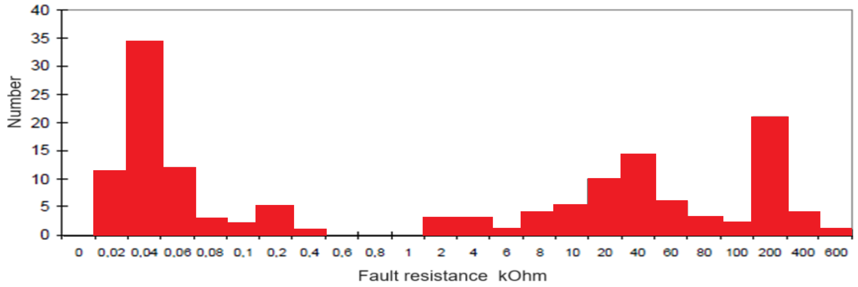
Figure 2.
Functional diagram of the centralized ground fault protection unit (CGFPU) in the 10 kV network with isolated neutral configuration.
Figure 2.
Functional diagram of the centralized ground fault protection unit (CGFPU) in the 10 kV network with isolated neutral configuration.
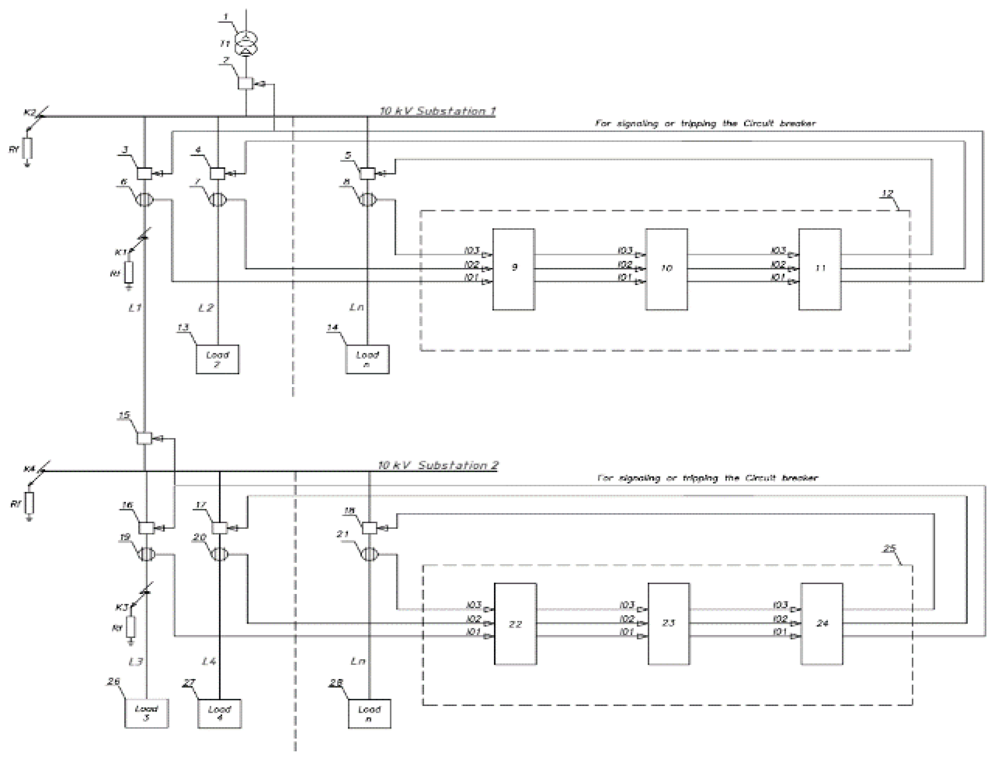
Figure 3.
Phasor diagram of the ground fault current and capacitive currents during a ground fault on an outgoing feeder.
Figure 3.
Phasor diagram of the ground fault current and capacitive currents during a ground fault on an outgoing feeder.
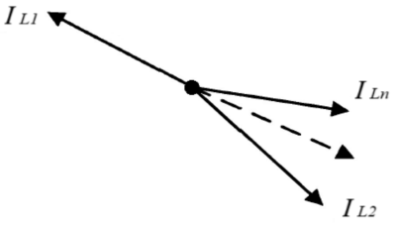
Figure 4.
Phasor diagram of zero-sequence currents during ground fault on the 10 kV busbars.
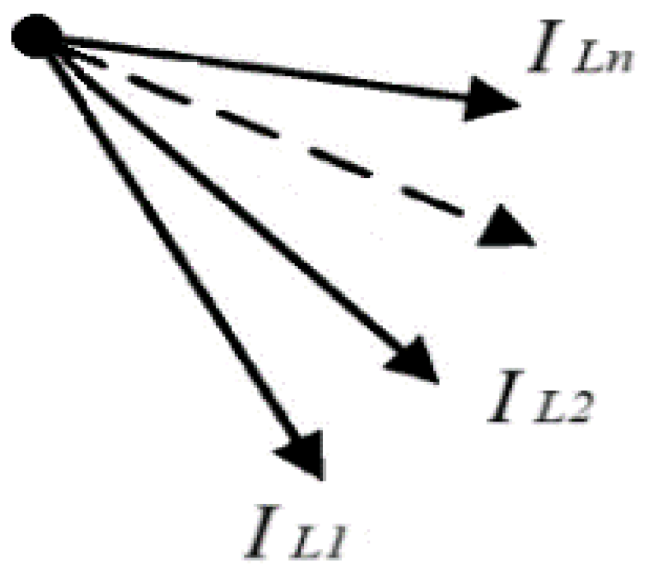
Figure 5.
Single-line diagram of a 110/10 kV substation in a network with isolated neutral configuration.
Figure 5.
Single-line diagram of a 110/10 kV substation in a network with isolated neutral configuration.
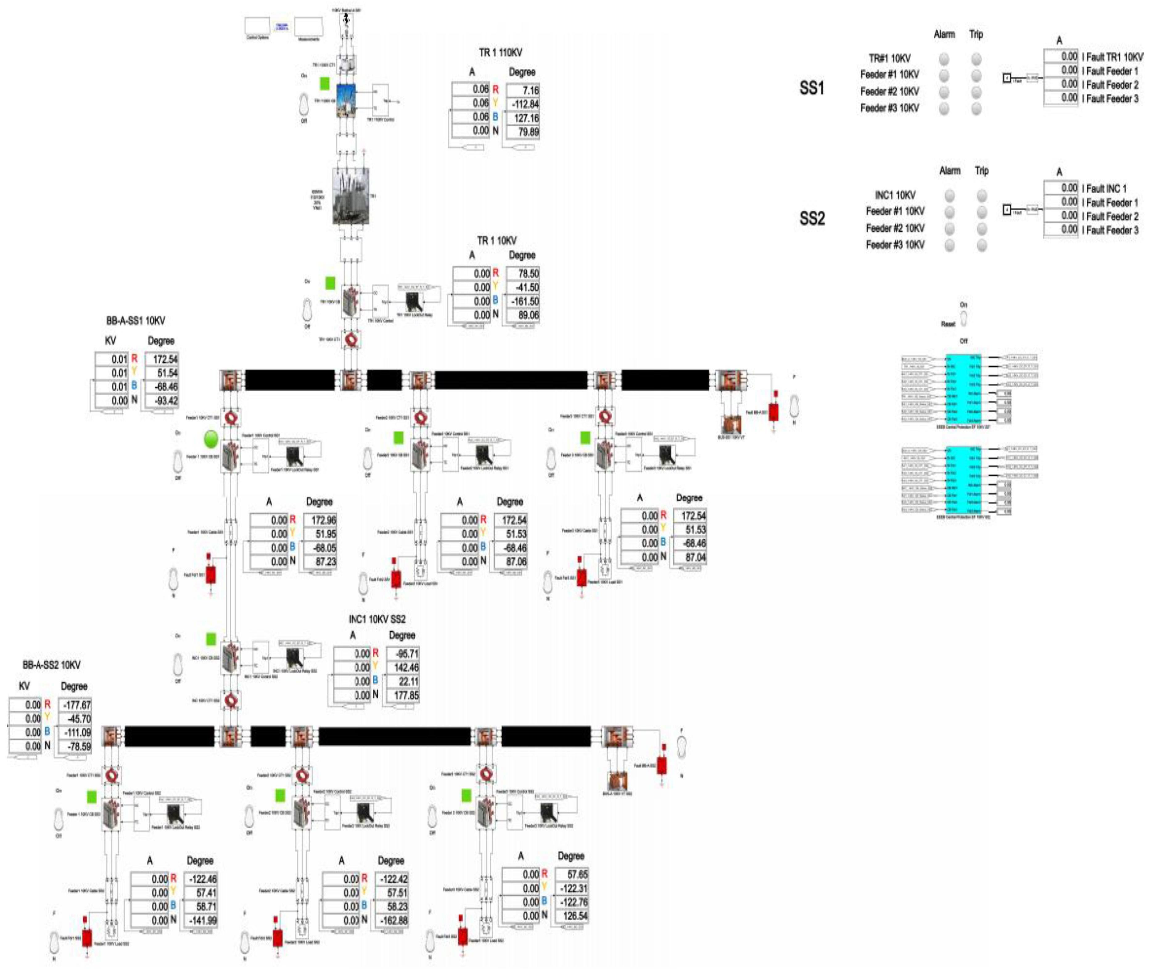
Figure 6.
Block diagram of the centralized ground fault protection unit (CGFPU) in a 10 kV network with isolated neutral configuration for substations No.1 and No. 2.
Figure 6.
Block diagram of the centralized ground fault protection unit (CGFPU) in a 10 kV network with isolated neutral configuration for substations No.1 and No. 2.
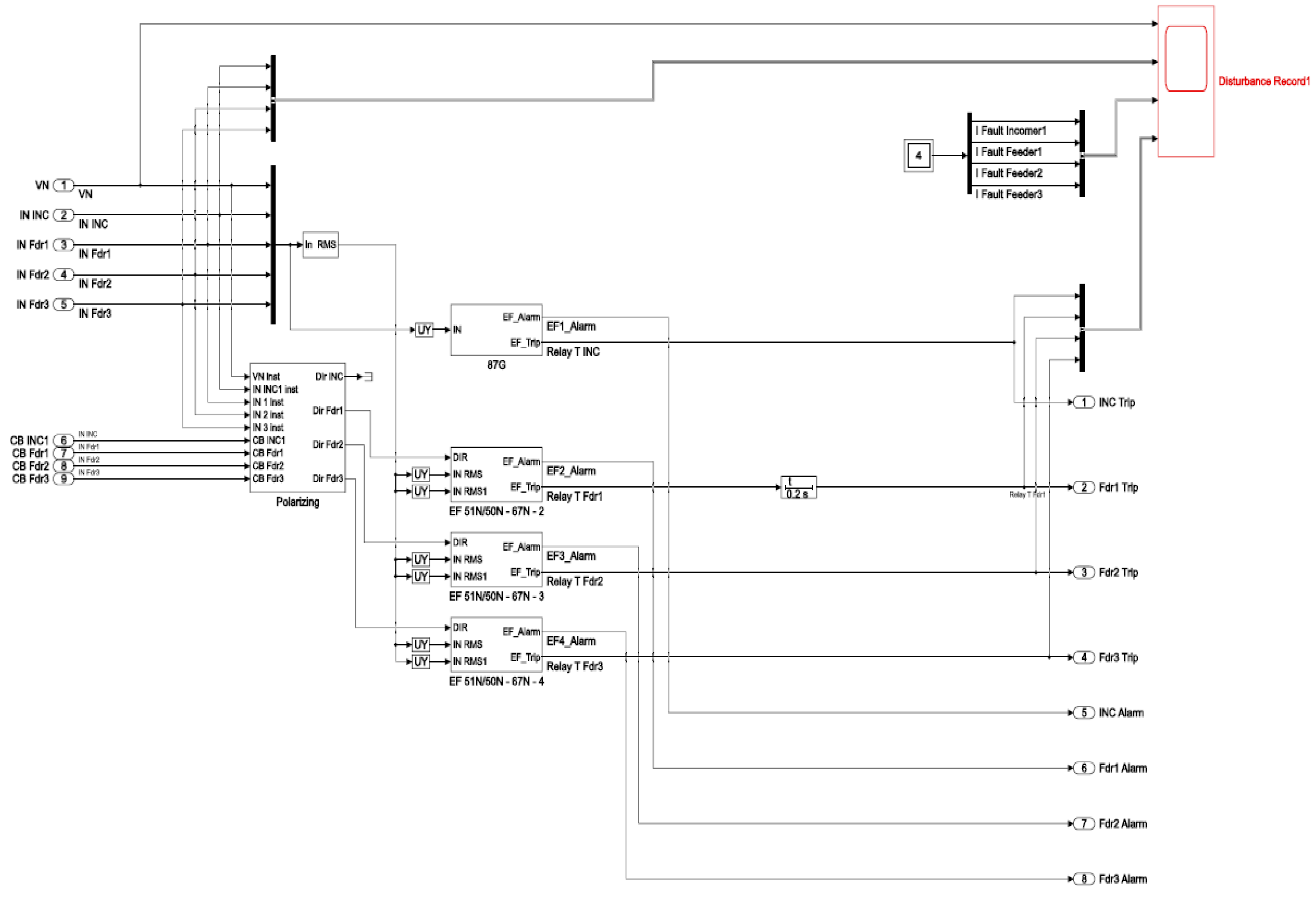
Figure 7.
Functional diagram of the CGFPU polarization module in the 10 kV network with isolated neutral configuration for substation No.1 and No. 2.
Figure 7.
Functional diagram of the CGFPU polarization module in the 10 kV network with isolated neutral configuration for substation No.1 and No. 2.
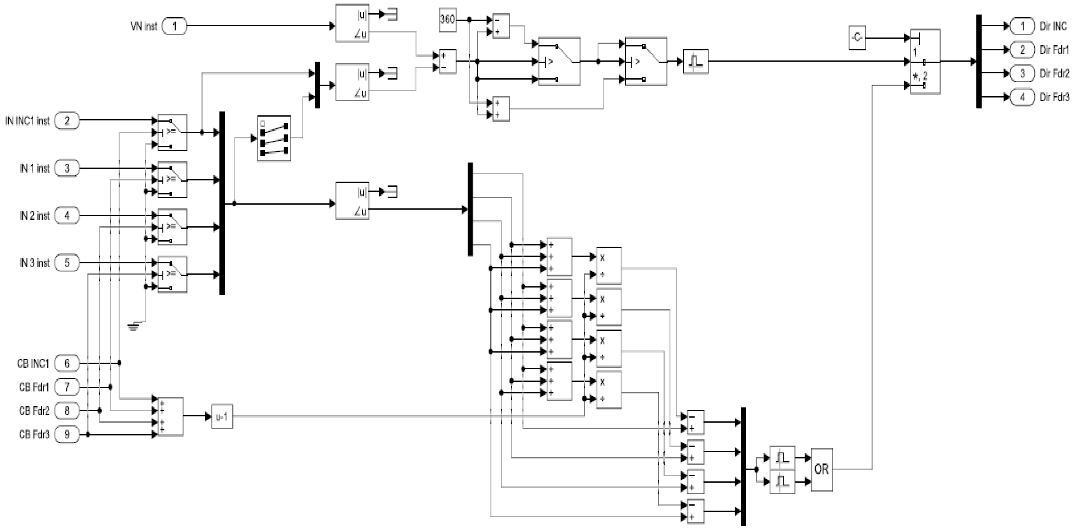
Figure 8.
Functional diagram of the angle and magnitude comparison module for feeders No.1, 2 and 3 in substations No.1 and No. 2.
Figure 8.
Functional diagram of the angle and magnitude comparison module for feeders No.1, 2 and 3 in substations No.1 and No. 2.
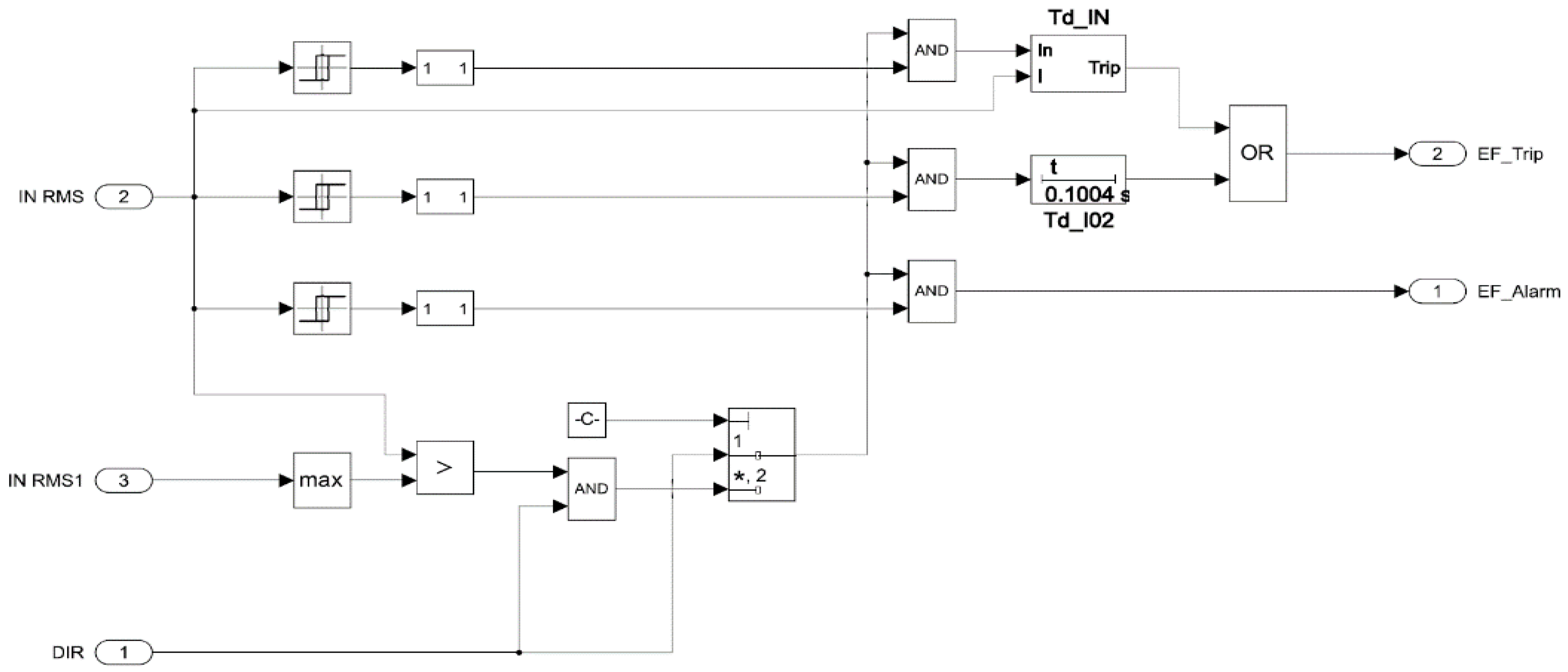
Figure 9.
Functional diagram of the magnitude and angle comparison module for the incomers in substations No.1 and No. 2.
Figure 9.
Functional diagram of the magnitude and angle comparison module for the incomers in substations No.1 and No. 2.
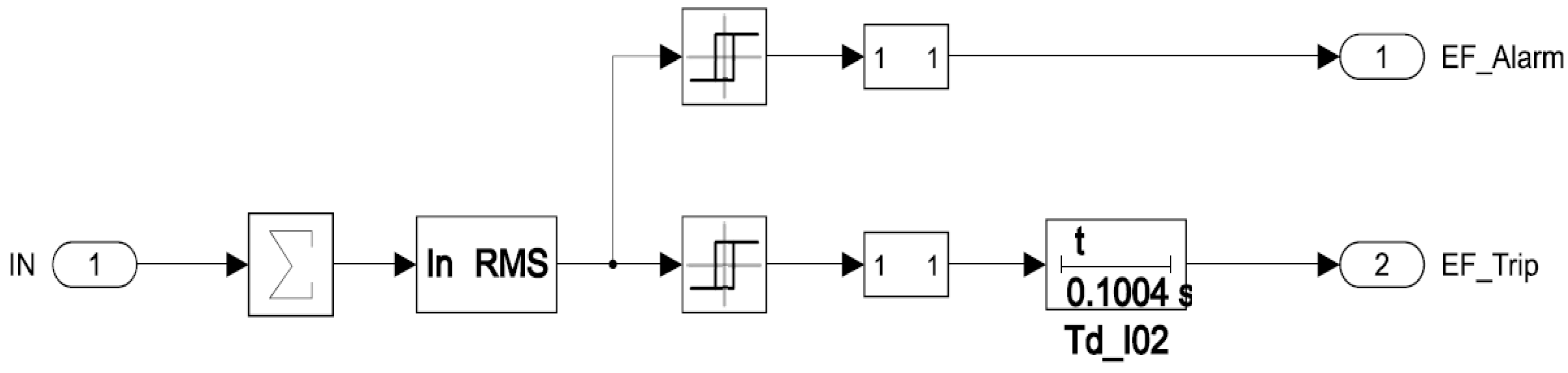
Figure 10.
10 kV distribution network with isolated neutral configuration.
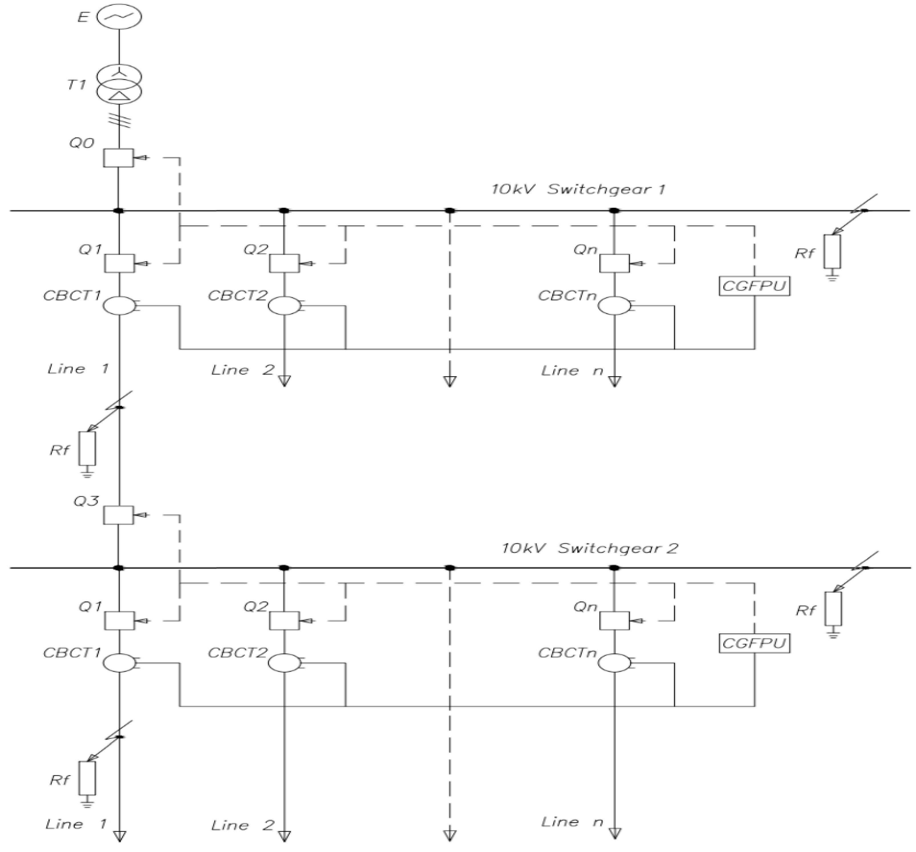
Figure 11.
Ground fault current with the transient resistance at feeder No.1, substation No.1, and capacitive currents in the 10 kV network with isolated neutral configuration.
Figure 11.
Ground fault current with the transient resistance at feeder No.1, substation No.1, and capacitive currents in the 10 kV network with isolated neutral configuration.
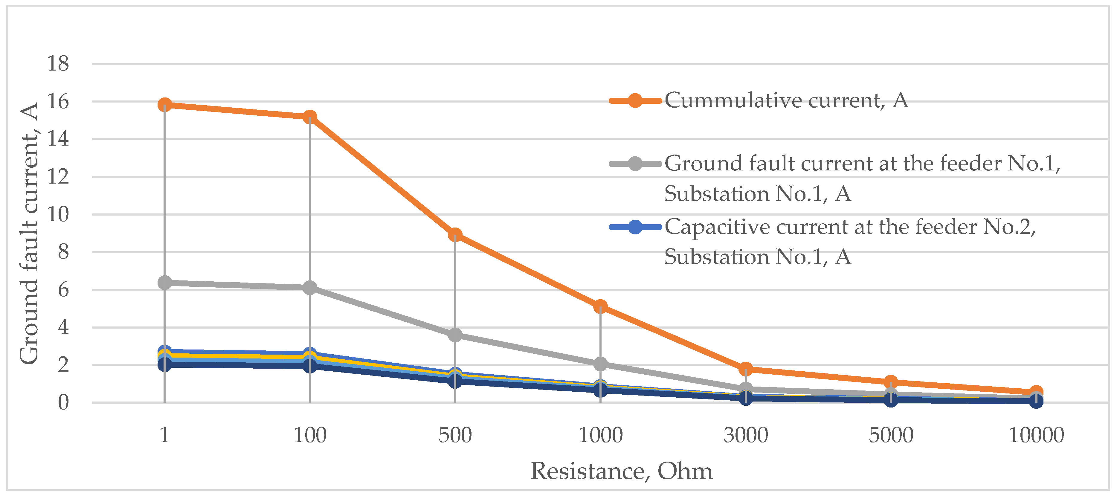
Figure 12.
Phasor diagram for the single-phase ground fault (SPGF) at feeder No.1, substation No.1, and capacitive currents in the 10 kV network with isolated neutral configuration.
Figure 12.
Phasor diagram for the single-phase ground fault (SPGF) at feeder No.1, substation No.1, and capacitive currents in the 10 kV network with isolated neutral configuration.
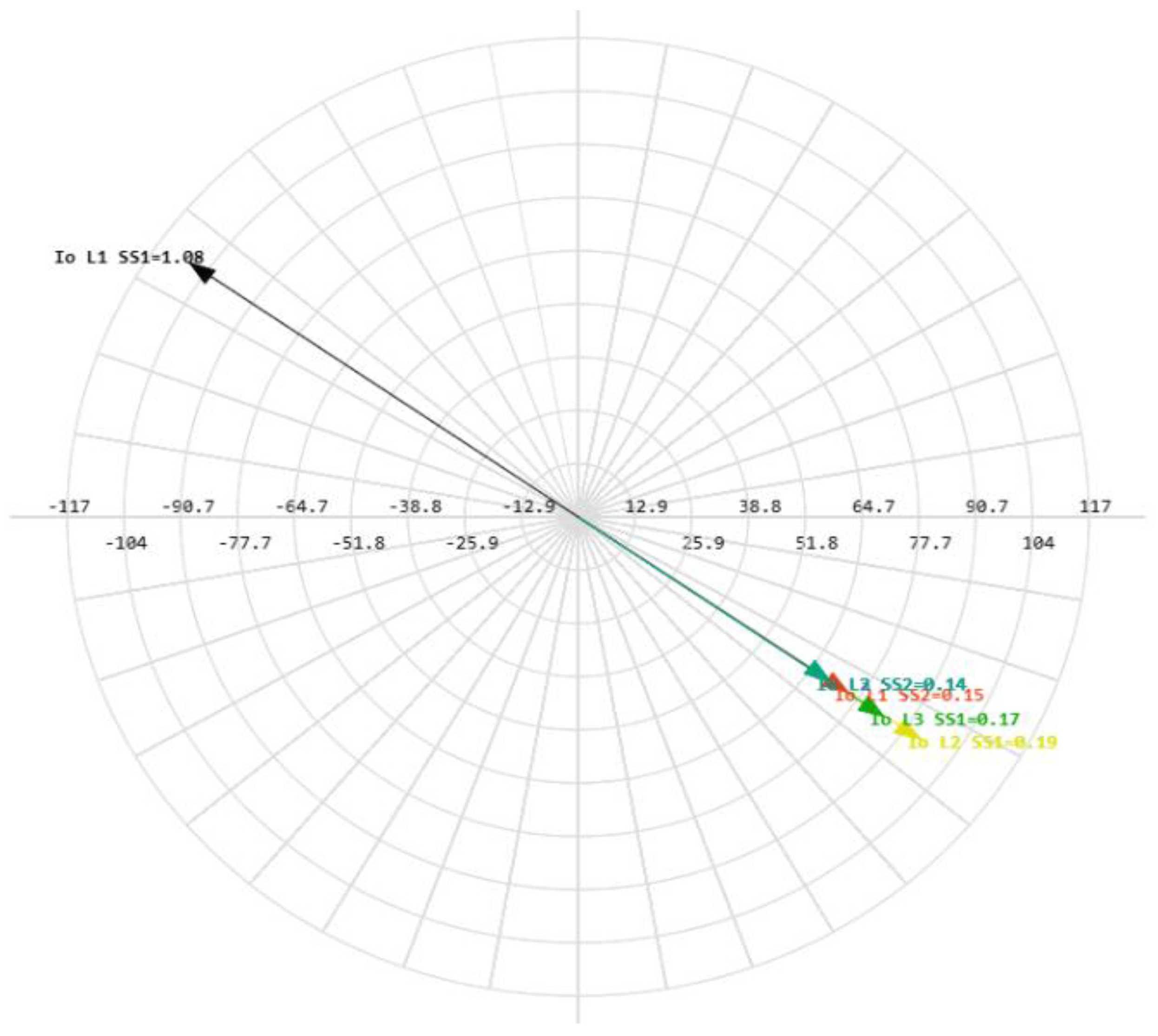
Figure 13.
Ground fault current with transient resistance on the substation No.1 bus and capacitive currents in the 10 kV network with isolated neutral configuration.
Figure 13.
Ground fault current with transient resistance on the substation No.1 bus and capacitive currents in the 10 kV network with isolated neutral configuration.
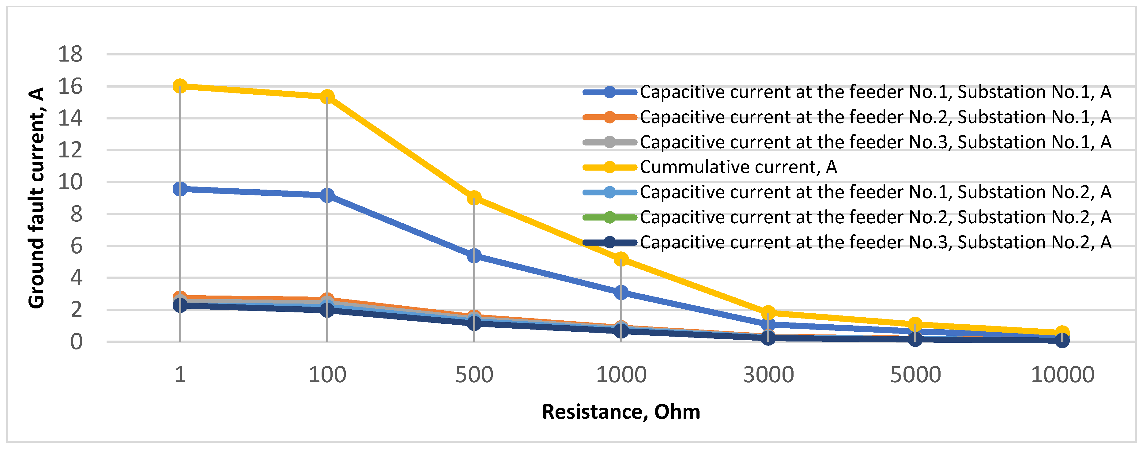
Figure 14.
Phasor diagram for the single-phase ground fault (SPGF) on the substation No.1 bus and capacitive currents in the 10 kV network with isolated neutral configuration.
Figure 14.
Phasor diagram for the single-phase ground fault (SPGF) on the substation No.1 bus and capacitive currents in the 10 kV network with isolated neutral configuration.
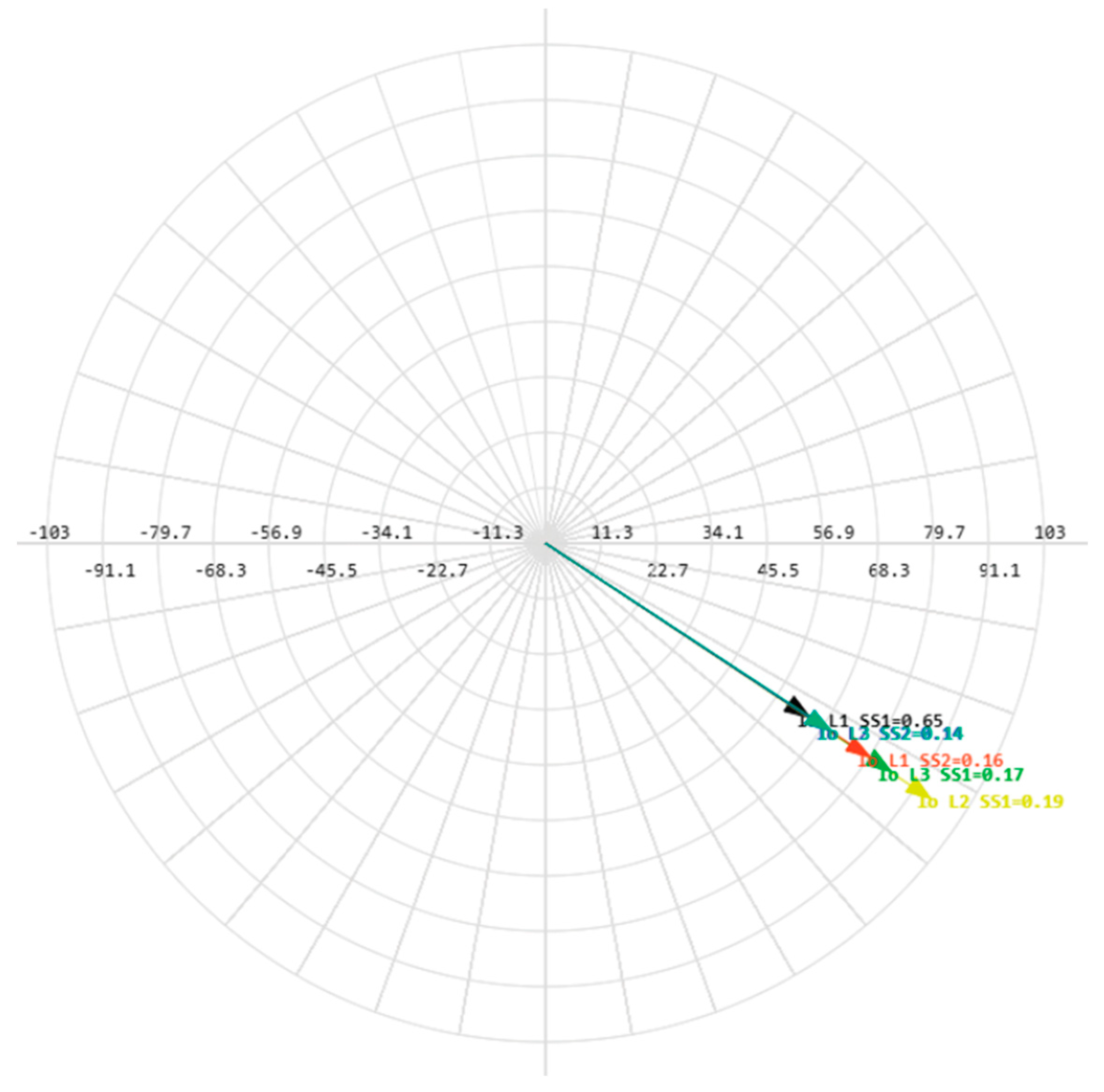
Figure 15.
Ground fault current with the transient resistance at feeder No.1, substation No.2, and capacitive currents in the 10 kV network with isolated neutral configuration.
Figure 15.
Ground fault current with the transient resistance at feeder No.1, substation No.2, and capacitive currents in the 10 kV network with isolated neutral configuration.
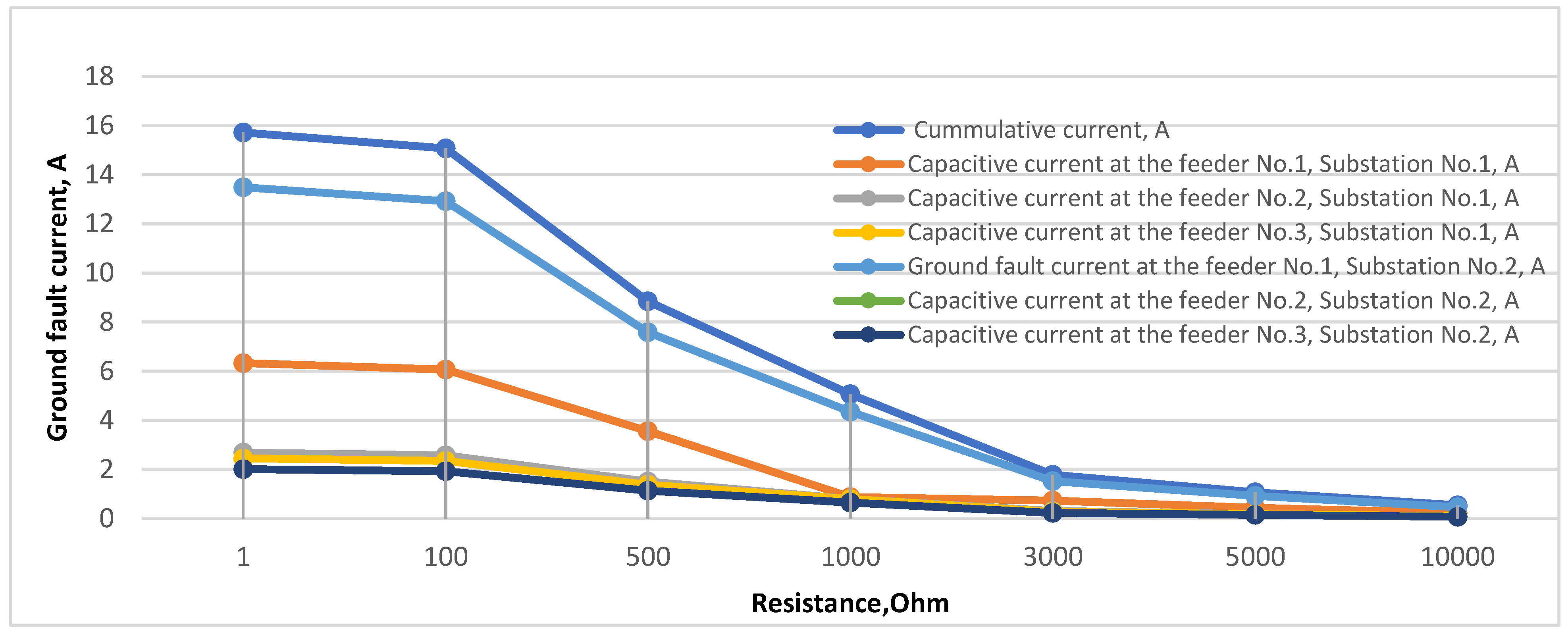
Figure 16.
Phasor diagram for the single-phase ground fault (SPGF) at feeder No.1, substation No.2, and capacitive currents in the 10 kV network with isolated neutral configuration.
Figure 16.
Phasor diagram for the single-phase ground fault (SPGF) at feeder No.1, substation No.2, and capacitive currents in the 10 kV network with isolated neutral configuration.
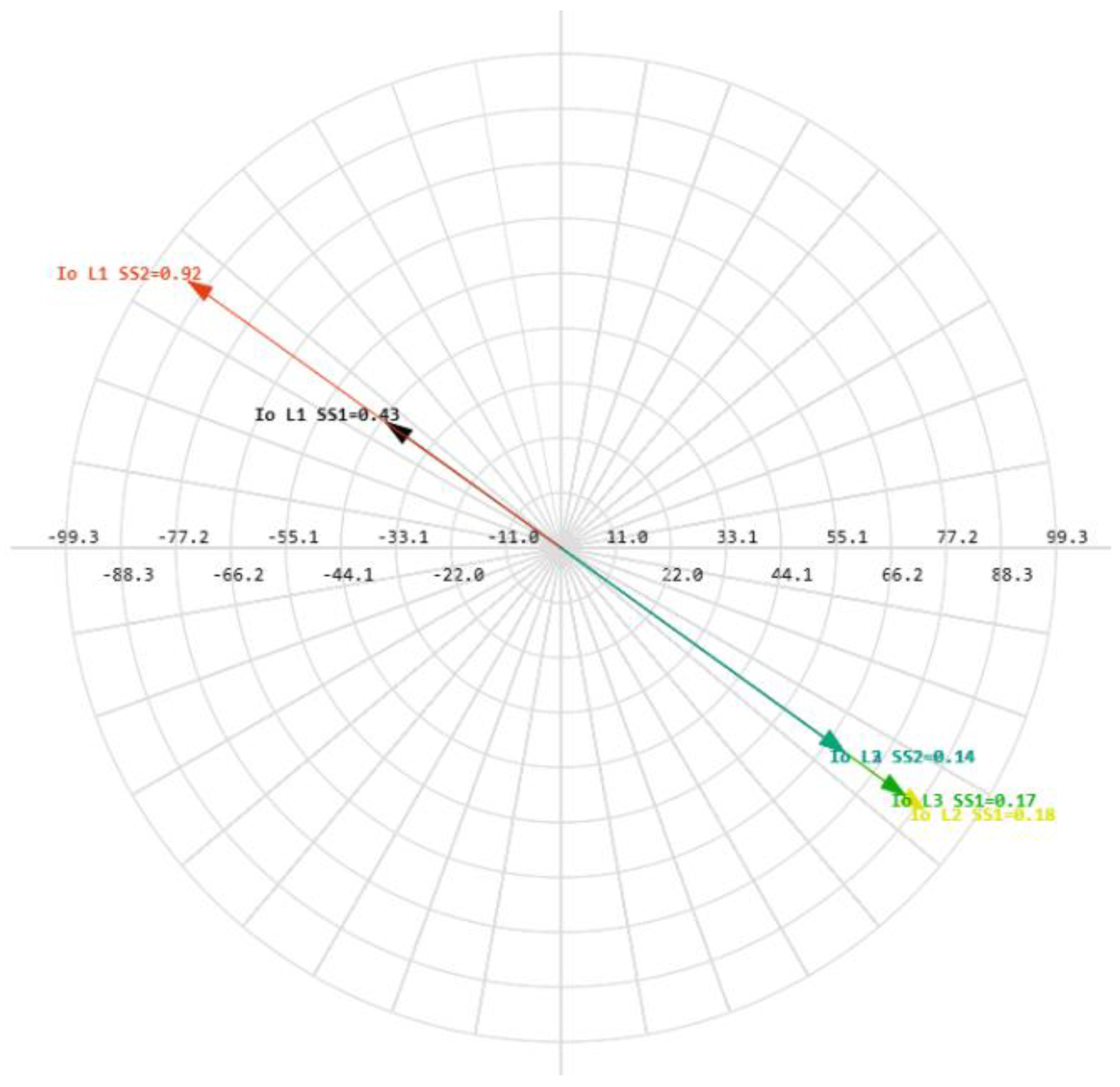
Figure 17.
Ground fault current with the transient resistance on the substation No.2 bus and capacitive currents in the 10 kV network with isolated neutral configuration.
Figure 17.
Ground fault current with the transient resistance on the substation No.2 bus and capacitive currents in the 10 kV network with isolated neutral configuration.
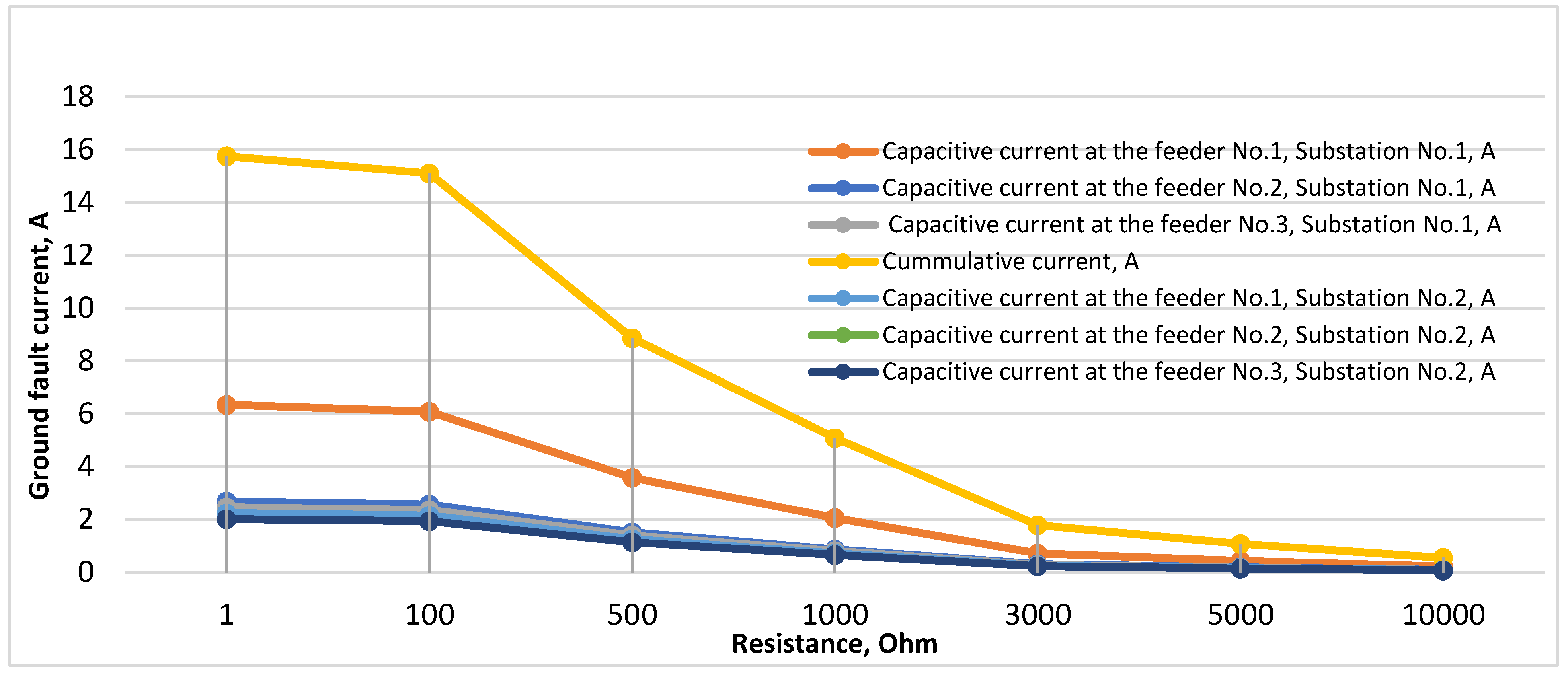
Figure 18.
Phasor diagram for the single-phase ground fault (SPGF) on the substation No.2 bus and capacitive currents in the 10 kV network with isolated neutral configuration.
Figure 18.
Phasor diagram for the single-phase ground fault (SPGF) on the substation No.2 bus and capacitive currents in the 10 kV network with isolated neutral configuration.

Figure 19.
demonstrates the disturbance recording of a single-phase ground fault (SPGF) with a transient resistance of Rf = 5000 Ohm at feeder No.1, substation No.1. The CGFPU accurately detects the ground fault, identifies the faulty feeder based on zero-sequence current magnitude and angle comparison, and selectively issues an alarm without nuisance trips of other feeders. This confirms the high sensitivity, selectivity, and operational reliability of the proposed protection scheme even in the presence of significant transient resistance.

Figure 20.
Presents the disturbance recording of a single-phase ground fault (SPGF) with a transient resistance of Rf= 5000 Ohm at feeder No.1, substation No.1 in the 10 kV network with isolated neutral configuration.
Figure 20.
Presents the disturbance recording of a single-phase ground fault (SPGF) with a transient resistance of Rf= 5000 Ohm at feeder No.1, substation No.1 in the 10 kV network with isolated neutral configuration.
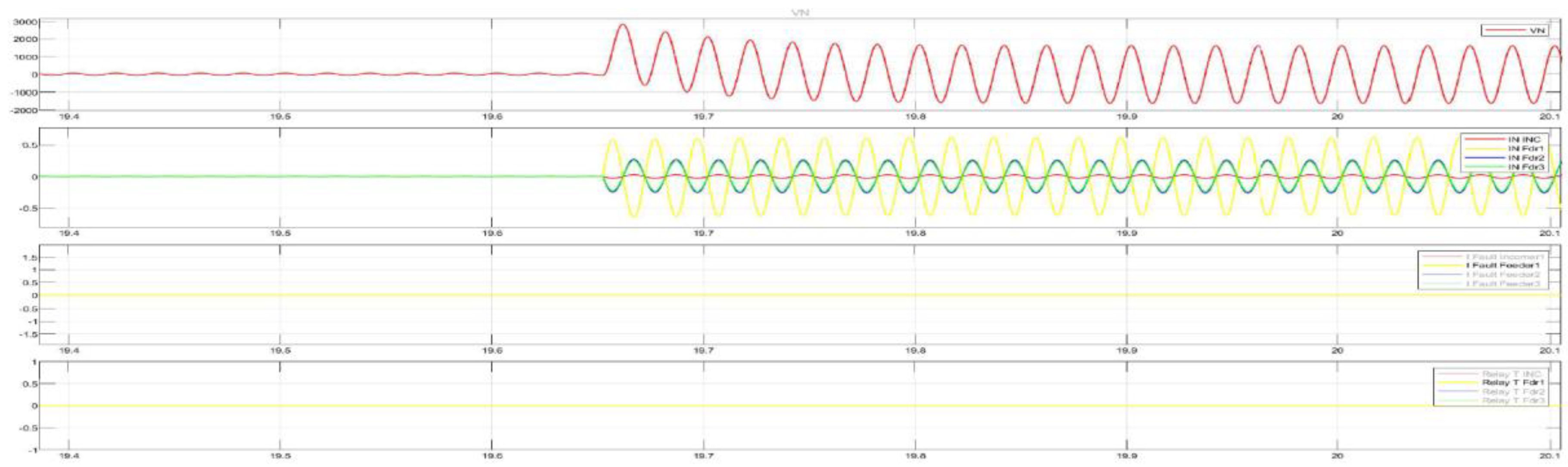
Figure 21.
Illustrates the correct detection and localization of a single-phase ground fault with a transient resistance of Rf = 5000 Ohm located on the substation No.1 bus. The CGFPU protection system correctly identifies the fault at the incomer by analyzing the magnitude and angle of the zero-sequence current and issues a selective alarm without false operation on unfaulted feeders, confirming high reliability and sensitivity even under high-resistance fault conditions.

Figure 22.
Disturbance record of (SPGF) with a transient resistance of Rf= 5000 Ohm on the substation No.1 bus in the 10 kV network with isolated neutral configuration.
Figure 22.
Disturbance record of (SPGF) with a transient resistance of Rf= 5000 Ohm on the substation No.1 bus in the 10 kV network with isolated neutral configuration.
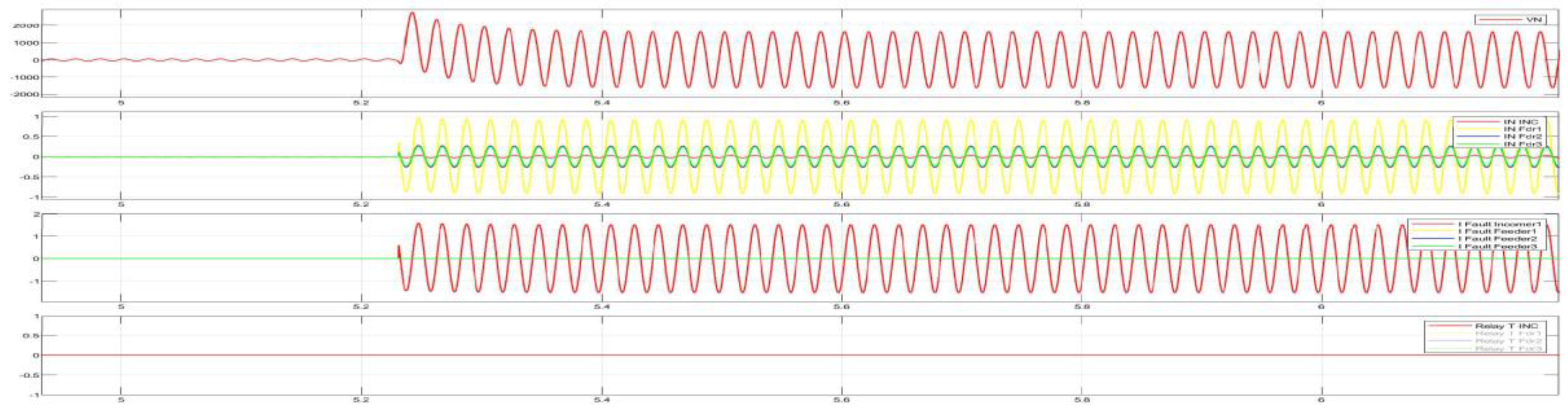
Figure 23.
Single line diagram with SPGF with the transient resistance of Rf = 5000 Ohm at the feeder No.1, substation No.2 in the 10 kV network with isolated neutral configuration.
Figure 23.
Single line diagram with SPGF with the transient resistance of Rf = 5000 Ohm at the feeder No.1, substation No.2 in the 10 kV network with isolated neutral configuration.
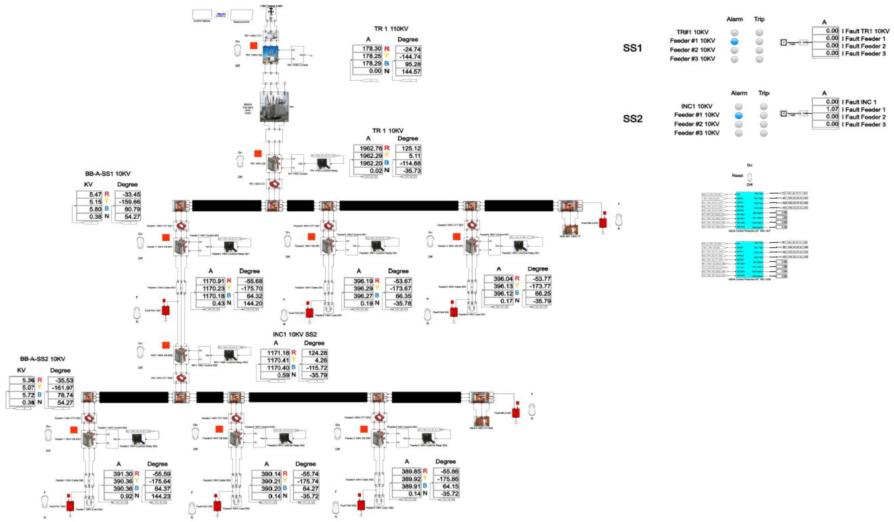
Figure 24.
Disturbance record of SPGF with the transient resistance of Rf= 5000 Ohm at the Feeder No.1, Substation No.2 in the 10 kV network with the isolated neutral configuration.
Figure 24.
Disturbance record of SPGF with the transient resistance of Rf= 5000 Ohm at the Feeder No.1, Substation No.2 in the 10 kV network with the isolated neutral configuration.
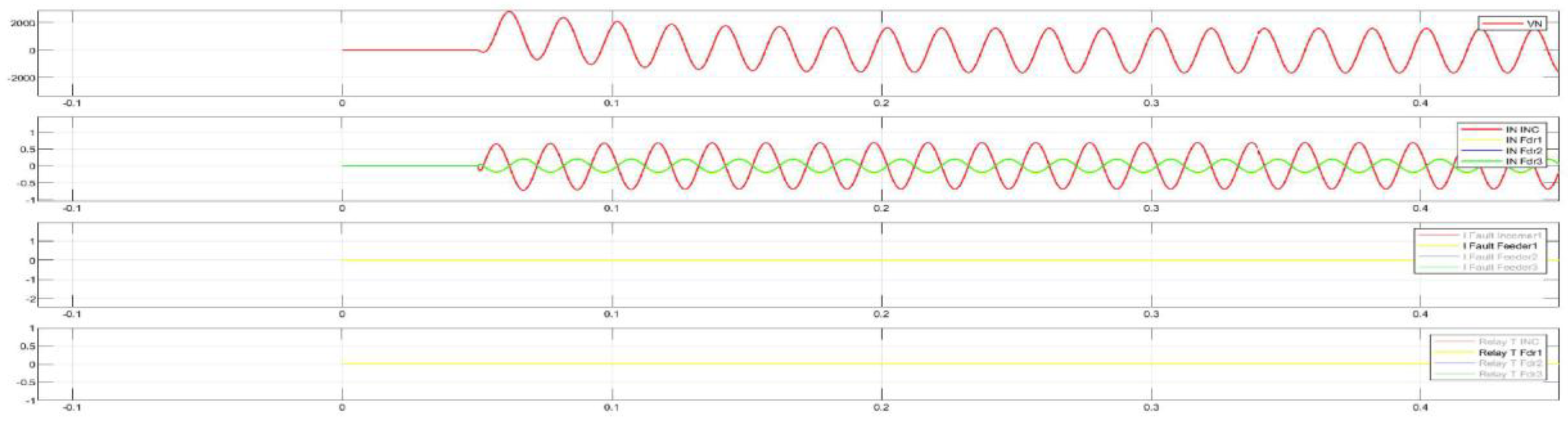
Figure 25.
Single line diagram with SPGF with the transient resistance of Rf = 5000 Ohm on the Substation No.2 bus in the 10 kV network with the isolated neutral configuration.
Figure 25.
Single line diagram with SPGF with the transient resistance of Rf = 5000 Ohm on the Substation No.2 bus in the 10 kV network with the isolated neutral configuration.
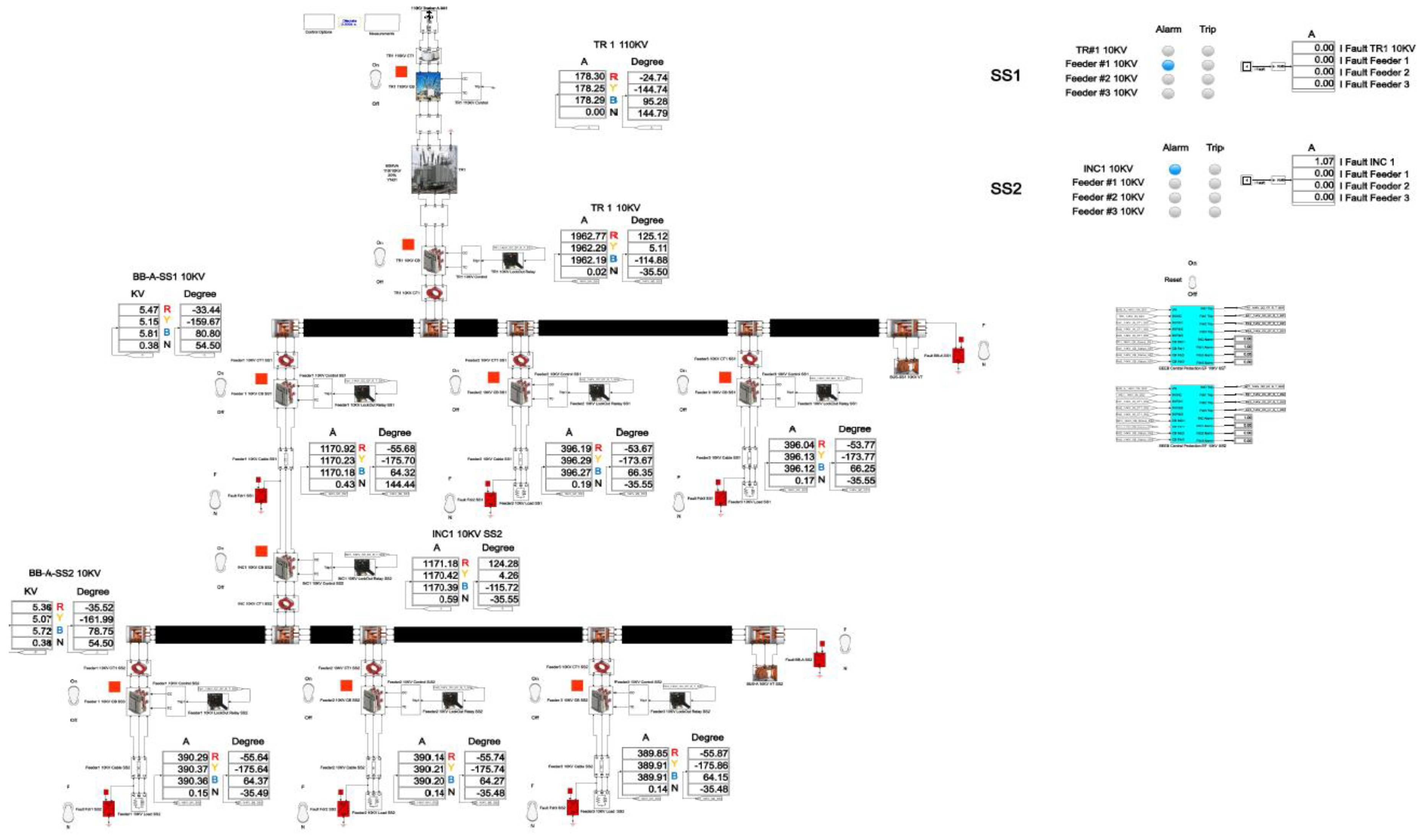
Figure 26.
Disturbance record of SPGF with the transient resistance of Rf= 5000 Ohm on the Substation No.2 bus in the 10 kV network with the isolated neutral configuration.
Figure 26.
Disturbance record of SPGF with the transient resistance of Rf= 5000 Ohm on the Substation No.2 bus in the 10 kV network with the isolated neutral configuration.
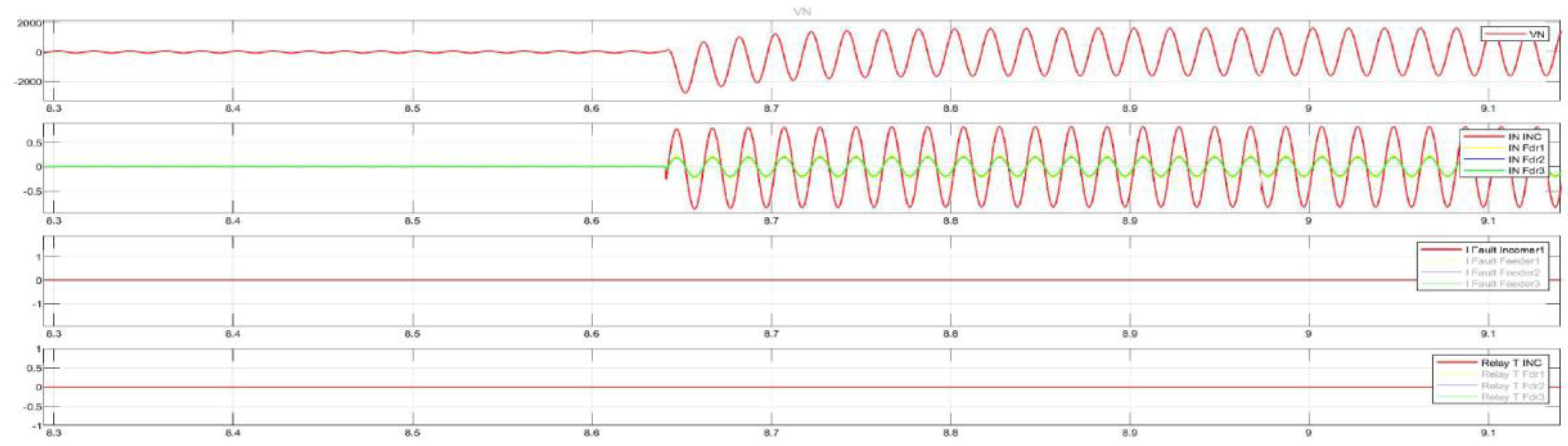
Figure 27.
Single line diagram with SPGF with the transient resistance of Rf = 1 Ohm at the Feeder No.1, Substation No.1 in the 10 kV network with the isolated neutral configuration (during SPGF).
Figure 27.
Single line diagram with SPGF with the transient resistance of Rf = 1 Ohm at the Feeder No.1, Substation No.1 in the 10 kV network with the isolated neutral configuration (during SPGF).

Figure 28.
Single line diagram with SPGF with the transient resistance of Rf = 1 Ohm at the Feeder No.1, Substation No.1 in the 10 kV network with the isolated neutral configuration (after clearing the ground fault).
Figure 28.
Single line diagram with SPGF with the transient resistance of Rf = 1 Ohm at the Feeder No.1, Substation No.1 in the 10 kV network with the isolated neutral configuration (after clearing the ground fault).
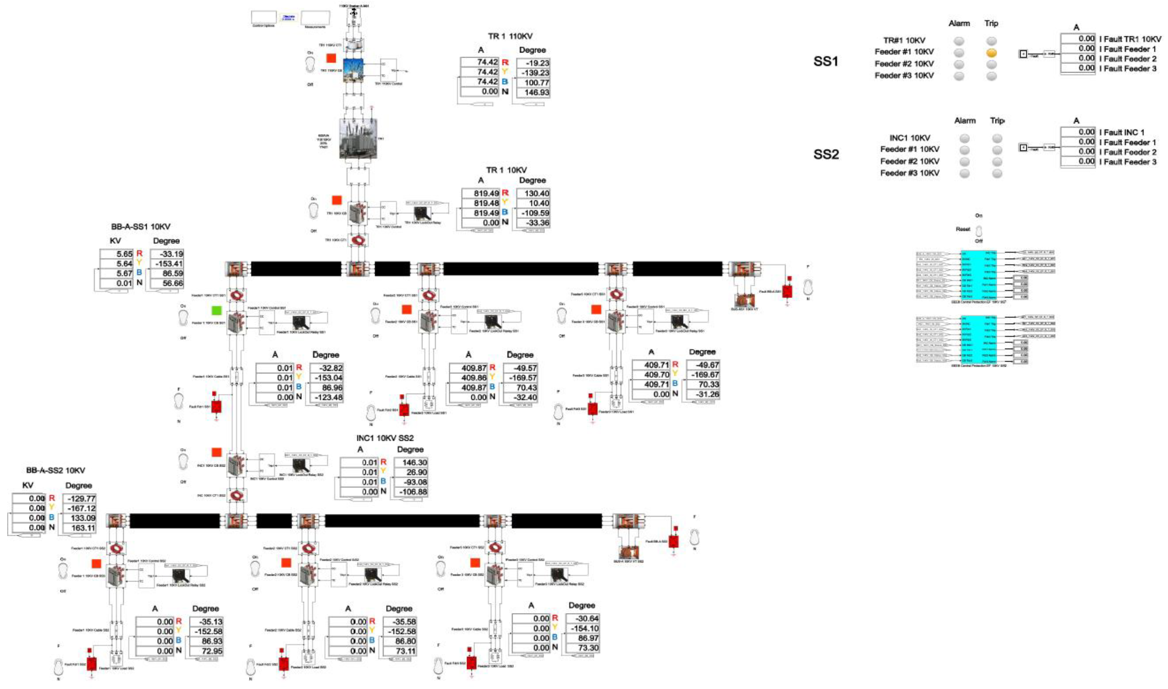
Figure 29.
Disturbance record of SPGF with the transient resistance of Rf= 1 Ohm at the Feeder No.1, Substation No.1 in the 10 kV network with the isolated neutral configuration.
Figure 29.
Disturbance record of SPGF with the transient resistance of Rf= 1 Ohm at the Feeder No.1, Substation No.1 in the 10 kV network with the isolated neutral configuration.
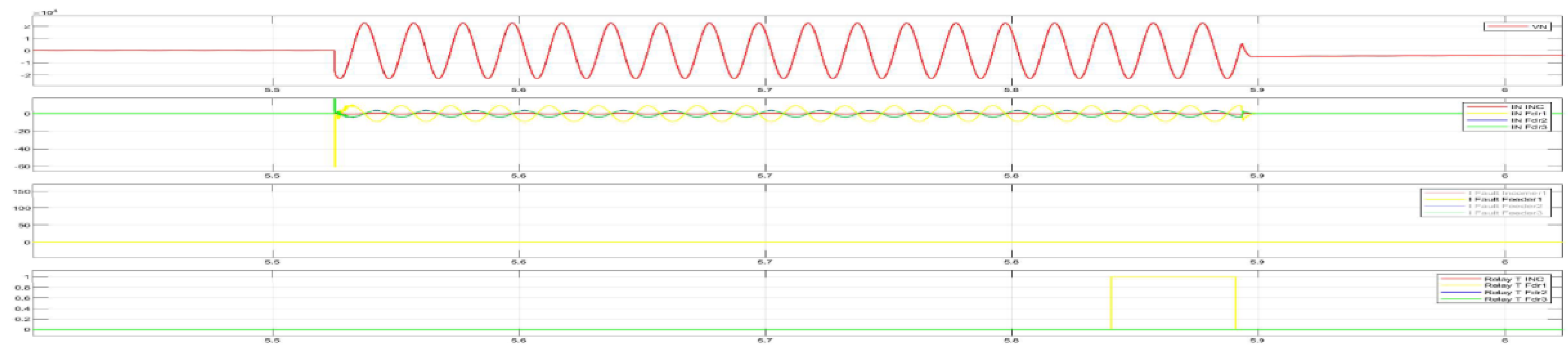
Figure 30.
Single line diagram with SPGF with the transient resistance of Rf = 1 Ohm on the Substation No.1 bus in the 10 kV network with the isolated neutral configuration (during SPGF).
Figure 30.
Single line diagram with SPGF with the transient resistance of Rf = 1 Ohm on the Substation No.1 bus in the 10 kV network with the isolated neutral configuration (during SPGF).
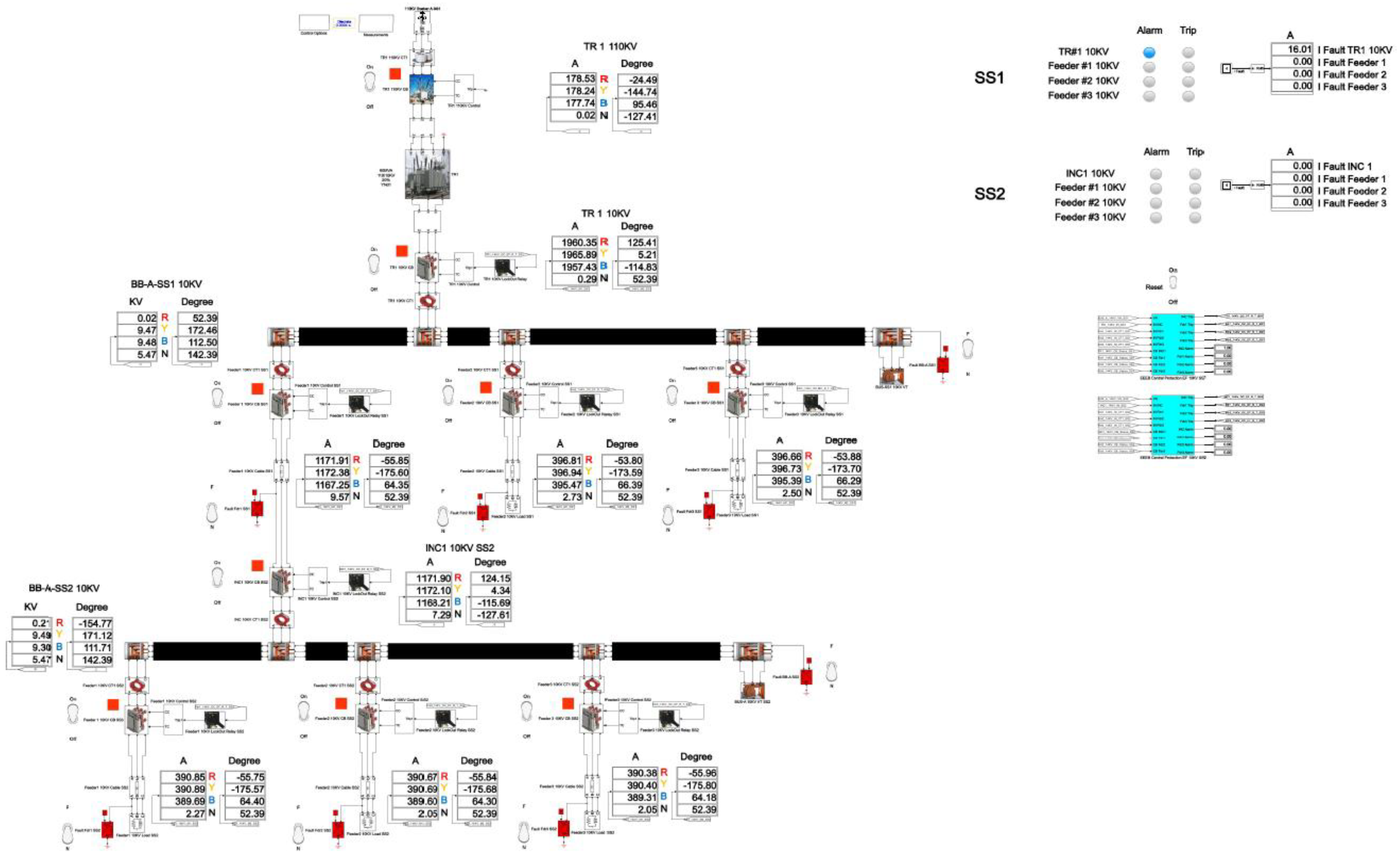
Figure 31.
Single line diagram with SPGF with the transient resistance of Rf = 1 Ohm on the Substation No.1 bus in the 10 kV network with the isolated neutral configuration (after clearing the ground fault).
Figure 31.
Single line diagram with SPGF with the transient resistance of Rf = 1 Ohm on the Substation No.1 bus in the 10 kV network with the isolated neutral configuration (after clearing the ground fault).
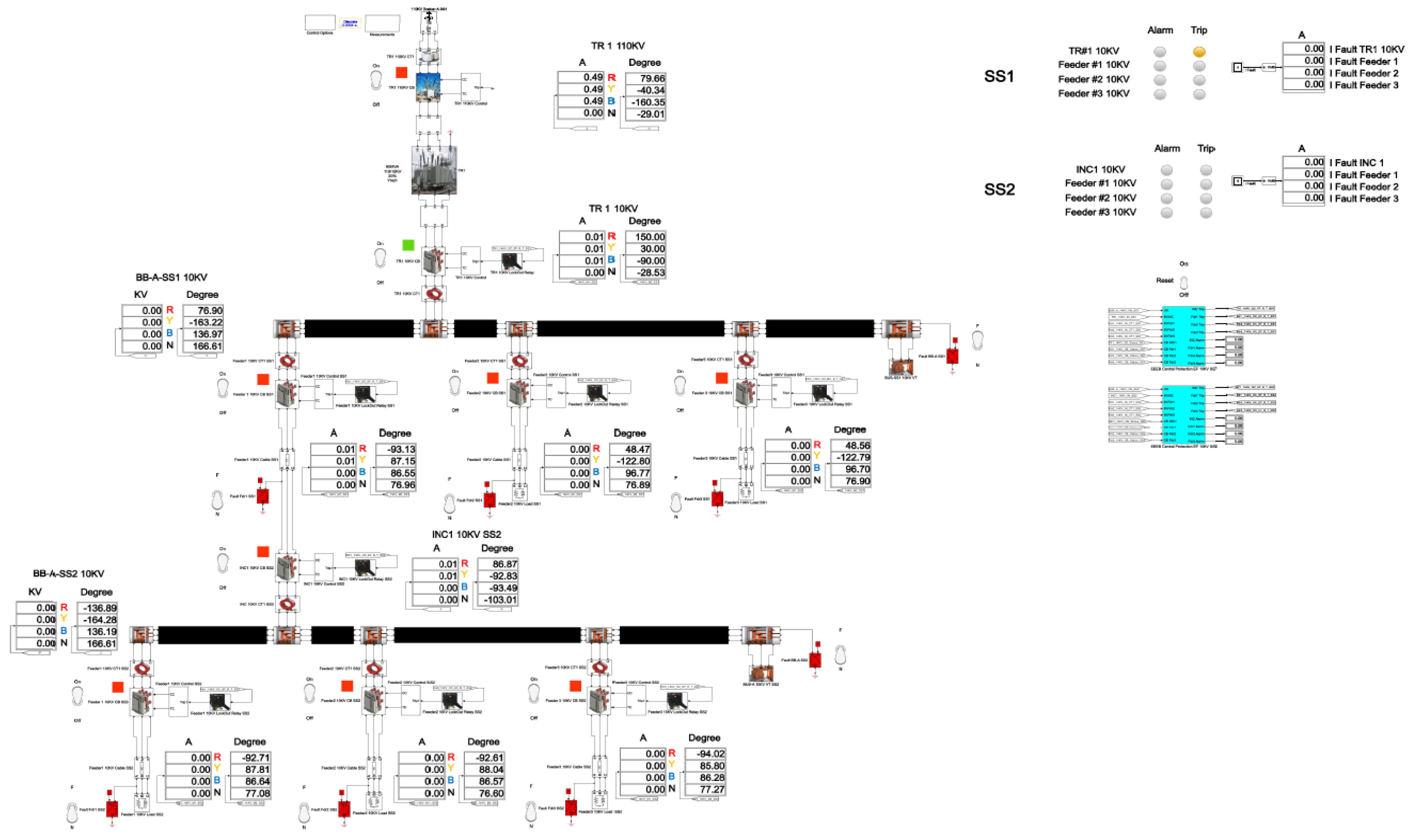
Figure 32.
Disturbance record of SPGF with the transient resistance of Rf= 1 Ohm on the Substation No.1 bus in the 10 kV network with the isolated neutral.
Figure 32.
Disturbance record of SPGF with the transient resistance of Rf= 1 Ohm on the Substation No.1 bus in the 10 kV network with the isolated neutral.
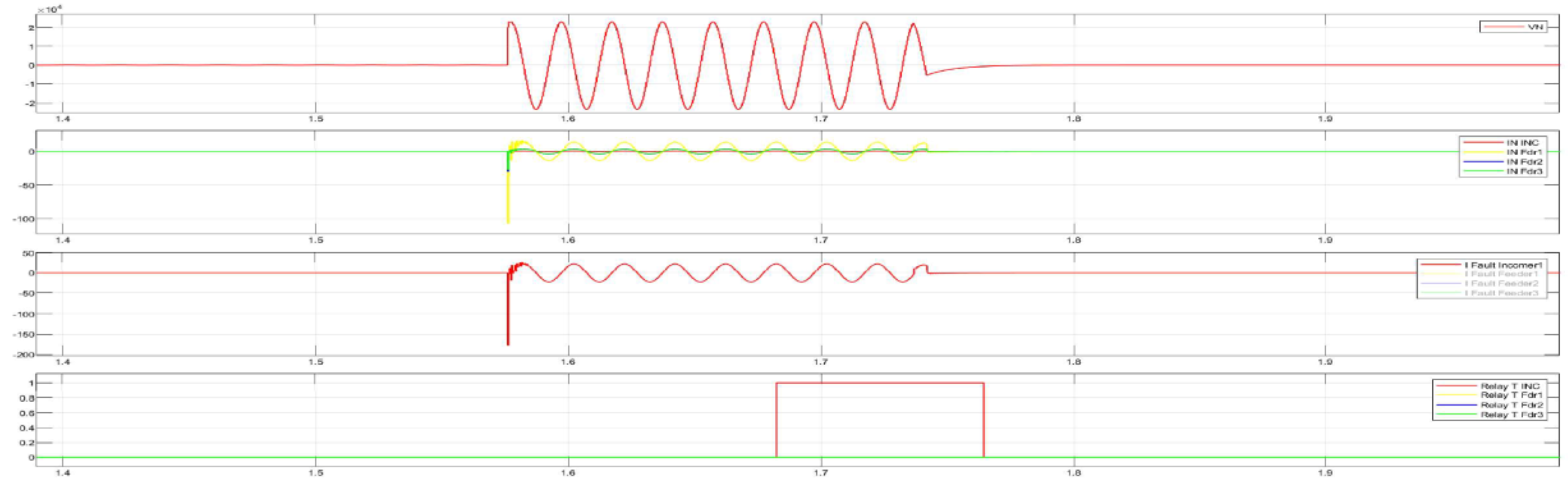
Figure 33.
Single line diagram with SPGF with the transient resistance of Rf = 1 Ohm at the Feeder No.1, Substation No.2 in the 10 kV network with the isolated neutral configuration (during SPGF).
Figure 33.
Single line diagram with SPGF with the transient resistance of Rf = 1 Ohm at the Feeder No.1, Substation No.2 in the 10 kV network with the isolated neutral configuration (during SPGF).
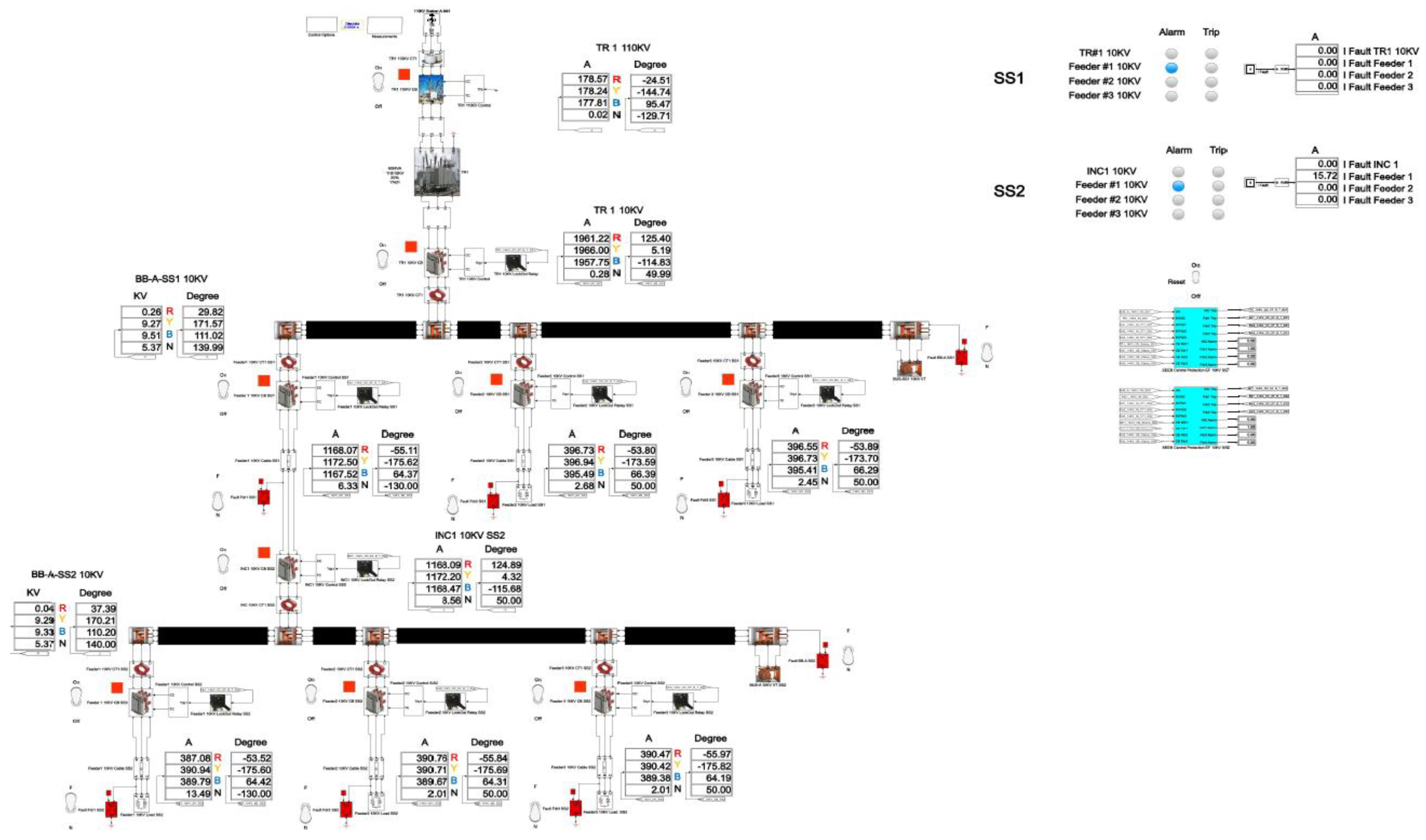
Figure 34.
Single line diagram with SPGF with the transient resistance of Rf = 1 Ohm at the Feeder No.1, Substation No.2 in the 10 kV network with the isolated neutral configuration (after clearing the ground fault).
Figure 34.
Single line diagram with SPGF with the transient resistance of Rf = 1 Ohm at the Feeder No.1, Substation No.2 in the 10 kV network with the isolated neutral configuration (after clearing the ground fault).
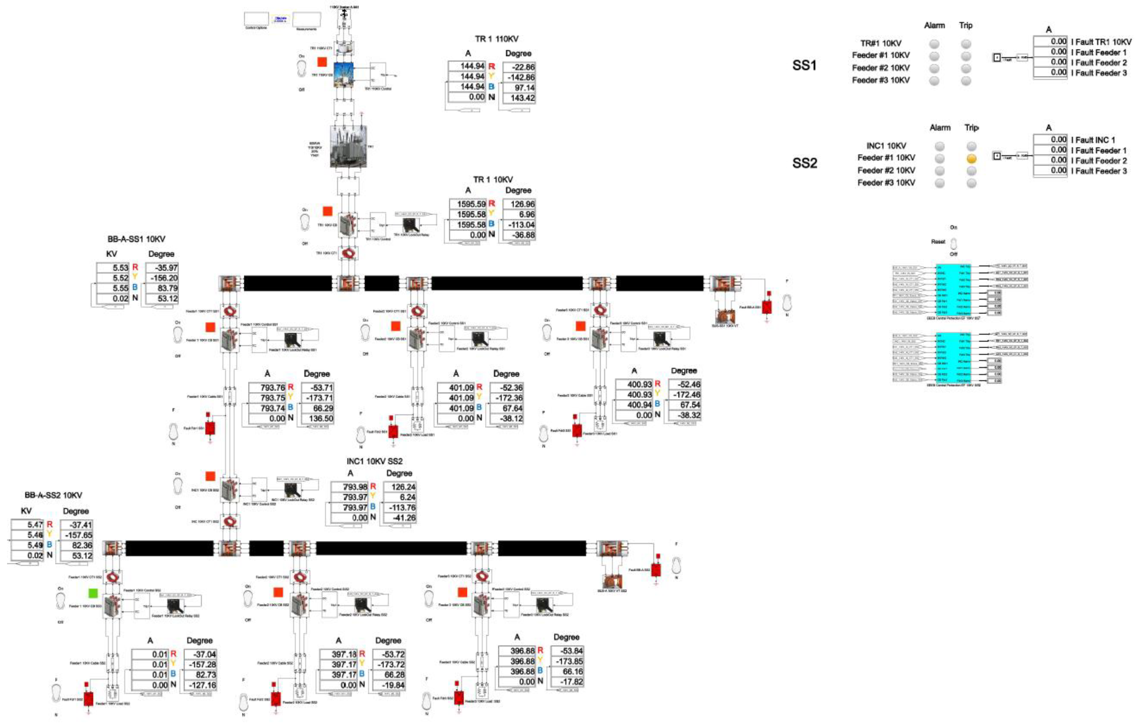
Figure 35.
Disturbance record of SPGF with the transient resistance of Rf= 1 Ohm at the Feeder No.1, Substation No.1 in the 10 kV network with the isolated neutral configuration.
Figure 35.
Disturbance record of SPGF with the transient resistance of Rf= 1 Ohm at the Feeder No.1, Substation No.1 in the 10 kV network with the isolated neutral configuration.
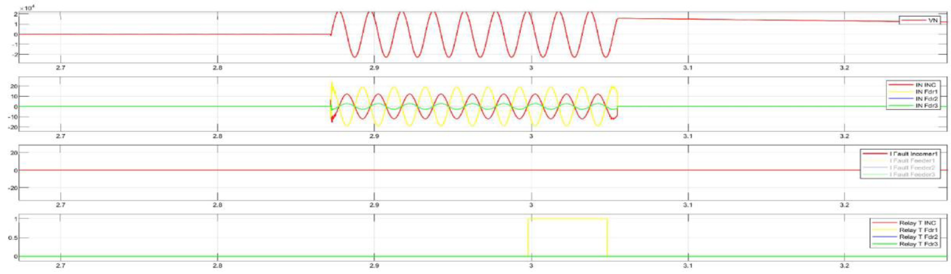
Figure 36.
Single line diagram with SPGF with the transient resistance of Rf = 1 Ohm on the Substation No.2 bus in the 10 kV network with the isolated neutral configuration (during SPGF).
Figure 36.
Single line diagram with SPGF with the transient resistance of Rf = 1 Ohm on the Substation No.2 bus in the 10 kV network with the isolated neutral configuration (during SPGF).
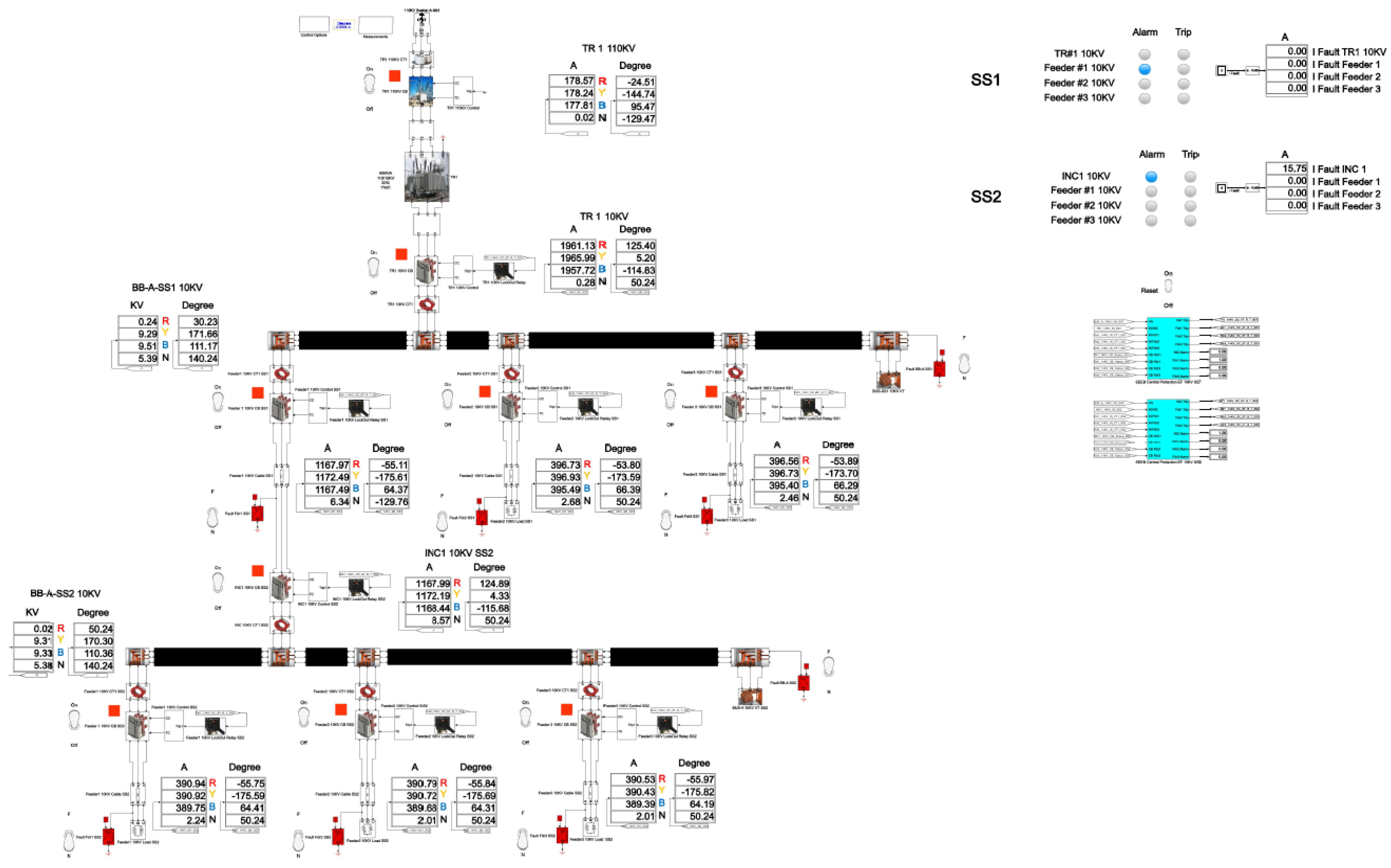
Figure 37.
Single line diagram with SPGF with the transient resistance of Rf = 1 Ohm on the Substation No.2 bus in the 10 kV network with the isolated neutral configuration (after clearing the ground fault).
Figure 37.
Single line diagram with SPGF with the transient resistance of Rf = 1 Ohm on the Substation No.2 bus in the 10 kV network with the isolated neutral configuration (after clearing the ground fault).
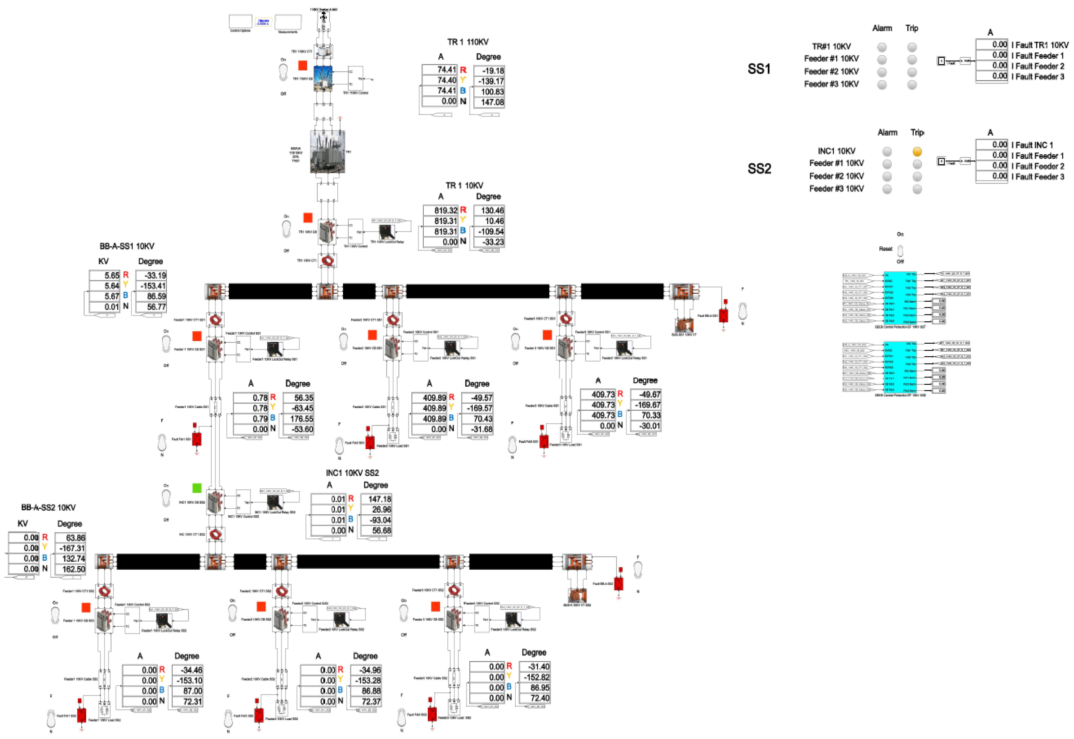
Figure 38.
Disturbance record of SPGF with the transient resistance of Rf= 1 Ohm on the Substation No.2 bus in the 10 kV network with the isolated neutral configuration.
Figure 38.
Disturbance record of SPGF with the transient resistance of Rf= 1 Ohm on the Substation No.2 bus in the 10 kV network with the isolated neutral configuration.
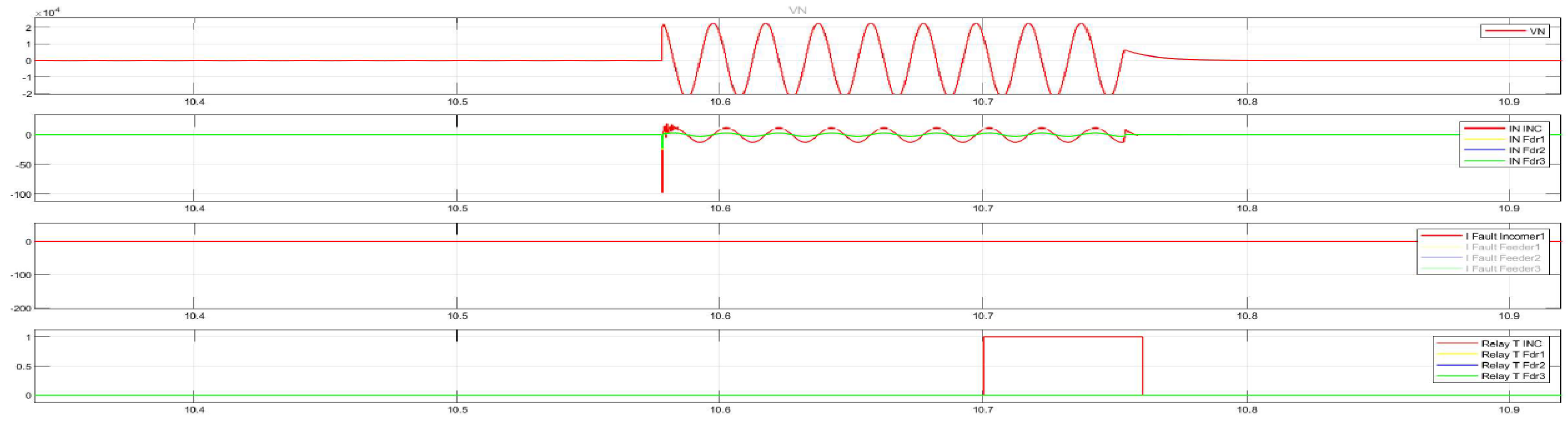

Table 1.
Single-phase ground fault (SPGF) current values at feeder No.1, substation No.1 for different transient resistances, and capacitive currents in the 10 kV network with isolated neutral configuration [26].
Table 1.
Single-phase ground fault (SPGF) current values at feeder No.1, substation No.1 for different transient resistances, and capacitive currents in the 10 kV network with isolated neutral configuration [26].
| No | Resistance Rf, Ohm | Cumulative current, A | Ground fault current at feeder No.1, substation No.1, A | Capacitive current at feeder No.2, substation No.1, A | Capacitive current at feeder No.3, substation No.1, A | Capacitive current at feeder No.1, substation No.2, A | Capacitive current at feeder No.2, substation No.2, A | Capacitive current at feeder No.3, substation No.2, A | |
|---|---|---|---|---|---|---|---|---|---|
| 1 | 1 | 15.82∠-129.02° | 6.37∠-129.02° | 2.69∠50.98° | 2.47∠50.98° | 2.25∠50.98° | 2.02∠50.98° | 2.02∠50.98° | |
| 2 | 100 | 15.17∠-145.16° | 6.10∠-145.16° | 2.58∠34.84° | 2.37∠34.84° | 2.15∠34.84° | 1.94∠34.84° | 1.94∠34.84° | |
| 3 | 500 | 8.91∠175.59° | 3.59∠175.59° | 1.52∠-4.41° | 1.39∠-4.41° | 1.27∠-4.40° | 1.14∠-4.40° | 1.14∠-4.40° | |
| 4 | 1000 | 5.11∠160.15° | 2.06∠160.15° | 0.87∠-19.85° | 0.80∠-19.85° | 0.73∠-19.84° | 0.65∠-19.84° | 0.65∠-19.84° | |
| 5 | 3000 | 1.79∠147.83° | 0.72∠147.78° | 0.31∠-32.21° | 0.28∠-32.21° | 0.25∠-32.17° | 0.23∠-32.17° | 0.23∠-32.17° | |
| 6 | 5000 | 1.08∠145.18° | 0.43∠145.18° | 0.19∠-34.81° | 0.17∠-34.81° | 0.15∠-34.75° | 0.14∠-34.74° | 0.14∠-34.73° | |
| 7 | 10000 | 0.54∠143.35° | 0.22∠143.18° | 0.09∠-36.79° | 0.09∠-36.79° | 0.08∠-36.67° | 0.07∠-36.65° | 0.07∠-36.64° |
Table 2.
Single-phase ground fault (SPGF) current values with different transient resistances at the substation No.1 bus and capacitive currents in the 10 kV network with isolated neutral configuration.
Table 2.
Single-phase ground fault (SPGF) current values with different transient resistances at the substation No.1 bus and capacitive currents in the 10 kV network with isolated neutral configuration.
| No. | Resistance Rf, Ohm | Cumulative current, A | Capacitive current at the Feeder No.1, Substation No.1, A | Capacitive current at the Feeder No.2, Substation No.1, A | Capacitive current at the Feeder No.3, Substation No.1, A | Capacitive current at the Feeder No.1, Substation No.2, A | Capacitive current at the Feeder No.2, Substation No.2, A | Capacitive current at the Feeder No.3, Substation No.2, A | |
|---|---|---|---|---|---|---|---|---|---|
| 1 | 1 | 16.01∠-127.61° | 9.57∠52.39° | 2.73∠52.39° | 2.50∠52.39° | 2.27∠52.39° | 2.27∠52.39° | 2.27∠52.39° | |
| 2 | 100 | 15.35∠-143.75° | 9.17∠36.25° | 2.62∠36.25° | 2.40∠36.25° | 2.18∠36.25° | 1.96∠36.25° | 1.96∠36.25° | |
| 3 | 500 | 9.02∠-177.01° | 5.39∠-2.99° | 1.54∠-3.00° | 1.41∠-3.00° | 1.28∠-2.99° | 1.15∠-2.99° | 1.15∠-2.99° | |
| 4 | 1000 | 5.17∠167.57° | 3.09∠-18.43° | 0.88∠-18.44° | 0.81∠-18.44° | 0.73∠-18.43° | 0.66∠-18.43° | 0.66∠-18.43° | |
| 5 | 3000 | 1.81∠149.24° | 1.08∠-30.77° | 0.31∠-30.81° | 0.28∠-30.81° | 0.26∠-30.77° | 0.23∠-30.76° | 0.23∠-30.76° | |
| 6 | 5000 | 1.09∠146.67° | 0.65∠-33.34° | 0.19∠-33.41° | 0.17∠-33.41° | 0.16∠-33.35° | 0.14∠-33.34° | 0.14∠-33.33° | |
| 7 | 10000 | 0.55∠144.77° | 0.33∠-35.26° | 0.09∠-35.41° | 0.09∠-35.40° | 0.08∠-35.28° | 0.07∠-35.25° | 0.07∠-35.24° |
Table 3.
Single-phase ground fault (SPGF) current values with different transient resistances at feeder No.1, substation No.2, and capacitive currents in the 10 kV network with isolated neutral configuration.
Table 3.
Single-phase ground fault (SPGF) current values with different transient resistances at feeder No.1, substation No.2, and capacitive currents in the 10 kV network with isolated neutral configuration.
| No. | Resistance Rf, Ohm | Cumulative current, A | Capacitive current at the Feeder No.1, Substation No.1, A | Capacitive current at the Feeder eder No.2, Substation No.1, A | Capacitive current at the Feeder No.3, Substation No.1, A | Ground fault current at the Feeder No.1, Substation No.2, A | Capacitive current at the Feeder No.2, Substation No.2, A | Capacitive current at the Feeder No.3, Substation No.2, A | |
|---|---|---|---|---|---|---|---|---|---|
| 1 | 1 | 15.72∠-130.00° | 6.33∠-130.00° | 2.68∠50.00° | 2.45∠50.00° | 13.49∠-130.00° | 2.01∠50.00° | 2.01∠50.00° | |
| 2 | 100 | 15.07∠-145.15° | 6.07∠-145.15° | 2.57∠33.85° | 2.35∠33.85° | 12.93∠-145.15° | 1.93∠33.85° | 1.93∠33.85° | |
| 3 | 500 | 8.85∠-5.40° | 3.56∠174.60° | 1.51∠-5.40° | 1.38∠-5.40° | 7.59∠-174.60° | 1.13∠-5.39° | 1.13∠-5.39° | |
| 4 | 1000 | 2.04∠159.16° | 0.87∠-20.84° | 0.79∠-20.84° | 0.79∠-20.84° | 4.35∠159.17° | 0.65∠-20.82° | 0.65∠-20.82° | |
| 5 | 3000 | 1.78∠33.19° | 0.72∠146.80° | 0.30∠-33.18° | 0.28∠-33.19° | 1.52∠146.83° | 0.23∠-33.15° | 0.23∠-33.14° | |
| 6 | 5000 | 1.07∠-35.79° | 0.43∠144.20° | 0.18∠-35.78° | 0.17∠-35.78° | 0.92∠144.24° | 0.14∠-35.72° | 0.14∠-35.71° | |
| 7 | 10000 | 0.54∠-37.77° | 0.22∠142.21° | 0.09∠-37.75° | 0.09∠-37.75° | 0.46∠-142.28° | 0.07∠-37.63° | 0.07∠-37.62° |
Table 4.
Single-phase ground fault (SPGF) current values with different transient resistances on the substation No.2 bus and capacitive currents in the 10 kV network with isolated neutral configuration.
Table 4.
Single-phase ground fault (SPGF) current values with different transient resistances on the substation No.2 bus and capacitive currents in the 10 kV network with isolated neutral configuration.
| No. | Resistance Rf, Ohm | Cummulative current, A | Capacitive current at the Feeder No.1, Substation No.1, A | Capacitive current at the Feeder No.2, Substation No.1, A | Capacitive current at the Feeder No.3, Substation No.1, A | Capacitive current at the Feeder No.1, Substation No.2, A | Capacitive current at the Feeder No.2, Substation No.2, A | Capacitive current at the Feeder No.3, Substation No.2, A | |
|---|---|---|---|---|---|---|---|---|---|
| 1 | 1 | 15.75∠50.24° | 6.34∠-129.76° | 2.68∠50.24° | 2.46∠50.24° | 2.24∠50.24° | 2.01∠50.24° | 2.01∠50.24° | |
| 2 | 100 | 15.10∠34.09° | 6.08∠-145.91° | 2.57∠34.09° | 2.36∠34.09° | 2.14∠34.10° | 1.93∠34.10° | 1.93∠34.10° | |
| 3 | 500 | 8.87∠-5.15° | 3.57∠174.85° | 1.51∠-5.15° | 1.39∠-5.15° | 1.26∠-5.15° | 1.13∠-5.15° | 1.13∠-5.15° | |
| 4 | 1000 | 5.08∠-20.60° | 2.05∠159.40° | 0.87∠-20.59° | 0.80∠-20.59° | 0.72∠-20.58° | 0.65∠-20.58° | 0.65∠-20.58° | |
| 5 | 3000 | 1.78∠-32.95° | 0.72∠147.04° | 0.31∠-32.95° | 0.28∠-32.95° | 0.25∠-32.91° | 0.23∠-32.91° | 0.23∠-32.91° | |
| 6 | 5000 | 1.07∠-35.55° | 0.43∠144.44° | 0.18∠-35.54° | 0.17∠-35.54° | 0.15∠-35.48° | 0.14∠-35.48° | 0.14∠-35.48° | |
| 7 | 10000 | 0.54∠-37.53° | 0.22∠142.45° | 0.09∠-37.51° | 0.09∠-37.51° | 0.08∠-37.40° | 0.07∠-37.39° | 0.07∠-37.39° |
Disclaimer/Publisher’s Note: The statements, opinions and data contained in all publications are solely those of the individual author(s) and contributor(s) and not of MDPI and/or the editor(s). MDPI and/or the editor(s) disclaim responsibility for any injury to people or property resulting from any ideas, methods, instructions or products referred to in the content. |
© 2025 by the authors. Licensee MDPI, Basel, Switzerland. This article is an open access article distributed under the terms and conditions of the Creative Commons Attribution (CC BY) license (http://creativecommons.org/licenses/by/4.0/).
Copyright: This open access article is published under a Creative Commons CC BY 4.0 license, which permit the free download, distribution, and reuse, provided that the author and preprint are cited in any reuse.


