
Submitted:
18 July 2025
Posted:
21 July 2025
You are already at the latest version
Abstract
This paper introduces a novel theoretical framework for energy conversion in natural flow systems, primarily focusing on ocean currents while extending its applicability to rivers and artificial channels. The proposed model is based on the concept of volumetric coupling between a conversion device and the surrounding incompressible flow. In contrast to classical approaches, which rely on axial deceleration and wake expansion, this method considers the interaction with an extended upstream volume of fluid whose inertia and continuity support energy extraction through controlled momentum deflection. This dynamic interaction is embedded within the Energy Restoration by Geophysical Fields (ERGF) model, which interprets these flows as open systems sustained by persistent physical mechanisms such as gravity, planetary rotation and thermohaline gradients in oceans, or topographic level differences in rivers and canals. Within this theoretical framework, the study analyses a resonant ideal turbine configuration designed to operate in continuous coupling with the flow, extracting mechanical power with minimal disturbance to large-scale hydrodynamics. Although experimental validation is ongoing, the paper outlines standardised testing methodologies (IEC, ITTC) that will underpin future performance assessments. The theoretical contributions presented herein aim to support the development of highly efficient and low-impact renewable energy systems based on volumetric interaction and continuous energy replenishment principles.
Keywords:
ocean current energy
; hydrokinetic turbines
; energy conversion in rivers and artificial channels
; volumetric-based energy extraction
; hydrodynamic coupling
; incompressible flow dynamics
; energy restoration model driven by geophysical fields
; experimental validation of turbines
1. Introduction
The global demand for renewable energy sources with high power density, low intermittency and reduced environmental impact has intensified the pursuit of new paradigms in energy conversion. Among the available natural resources, liquid flows in both natural and artificial settings, such as ocean currents, rivers and canals, present a vast yet underexploited potential for kinetic energy extraction [1].
In this study, the term "ocean currents" is used in a broad sense. It encompasses both large-scale permanent planetary flows, such as the Gulf Stream, and periodic tidal currents. These environments share fundamental physical properties, including high density and incompressibility. These characteristics distinguish them from atmospheric flows like wind and enable hydrokinetic conversion approaches that can generate significant power even at moderate flow velocities [2].
However, most current technologies used for this purpose derive from wind turbines, originally designed for compressible, low-density fluids. When applied to liquid media, particularly in marine systems, traditional models that rely on axial flow deceleration and wake expansion face important limitations. Recent studies have shown that single-rotor turbines based on the wind paradigm do not adequately represent the hydrodynamic behaviour of dense liquid flows, especially in oceanic contexts [3]. This reinforces the need for alternative approaches.
International reports highlight the growing global interest in the sustainable exploitation of ocean currents as a renewable energy source [4]. In parallel, researchers have employed advanced optimisation techniques, such as artificial neural networks, to refine the geometry of hydrokinetic turbines [5], overcoming performance limitations of conventional designs.
This work proposes volumetric coupling as the primary mechanism for energy conversion in incompressible flows, such as ocean currents, rivers and artificial channels. Unlike traditional approaches that rely on local flow deceleration at the turbine area, volumetric coupling assumes a continuous interaction with an extended upstream volume of fluid. This moving mass transfers momentum to the rotor, whose geometry imposes a gradual deflection on the velocity vector. In doing so, part of the flow's energy is converted into mechanical torque without requiring local flow deceleration or wake expansion.
To ensure the sustainability of this energy conversion process, the model is grounded in the concept of Energy Restoration by Geophysical Fields (ERGF). This theoretical framework treats natural flows as open systems continuously driven by geophysical fields, including gravity, Earth's rotation and thermohaline gradients in oceans, or topographic elevation differences in rivers and canals. These mechanisms maintain the persistent movement of liquid masses and provide, along the flow, the energy required to sustain large-scale motion. A converter properly coupled to this system can redirect part of the momentum supported by such fields into mechanical energy, without compromising hydrodynamic coherence or flow continuity.
To make this hypothesis of volumetrically sustained energy conversion viable, a specific converter configuration is proposed. This configuration, referred to as the ideal turbine, is conceived as a resonant system capable of operating in dynamic synchrony with the flow. In this context, "resonance" does not imply classical oscillatory behaviour. Instead, it refers to the capacity to maintain a stable coupling with the upstream fluid mass, thereby enabling continuous conversion without significant hydrodynamic disturbances.
By imposing a gradual deflection of up to 90 degrees on the velocity vector along its blades, the ideal turbine redirects the momentum of the coupled upstream fluid volume, converting it into rotational torque. This conversion occurs without significant obstruction of the flow and with only a slight axial reduction, which remains compatible with regimes supported by geophysical fields. Although the device interacts with a considerable fluid volume, it generates mechanical work through the resultant force from the vectorial deflection of the fluid momentum. It does so without requiring punctual deceleration and without causing large-scale hydrodynamic disruption, although a local reorganisation of the downstream flow does occur, induced by the deflection imposed by the turbine blades.
This conversion approach enables continuous energy generation while preserving the natural hydrodynamic regime of the current. It minimises environmental impact on aquatic ecosystems and supports stable and enduring operation. The principle of volumetric energy conversion, based on dynamic coupling between the device and the flow, as predicted by the ERGF model, lays the foundation for a new class of high-efficiency, low-impact marine energy systems designed to operate in harmony with natural ocean circulation patterns.
Although focused primarily on ocean currents, the model is also conceptually applicable to rivers and artificial channels, provided the specific sustaining mechanisms of those flows are considered, such as topographic gradients or dam-controlled discharges.
2. Combined Theoretical Framework
2.1. Limitations of the Classical Betz Model in Incompressible Media
The classical model for energy conversion in open flows, proposed by Albert Betz in 1919, establishes that the energy extracted by a turbine is directly related to the reduction in flow velocity as it passes through the rotor. To ensure mass conservation, the model assumes that this reduction in velocity must be compensated by an expansion of the downstream wake. This allows the flow to continue at a reduced velocity through an area of increased cross-sectional size. This assumption is widely adopted in the design of marine current turbines, which are often based on wind turbine principles [6].
This reasoning leads to the Betz limit, which defines the theoretical maximum power extractable from a free-stream flow as:
where is the fluid density, A is the rotor swept area, and v is the free-stream velocity.
This equation (1) is based on the continuity equation, which requires that the mass entering the turbine must continue downstream, even at a reduced velocity. In Betz's model [7], the fluid is treated as incompressible, meaning that any reduction in velocity must necessarily be accompanied by an expansion of the flow area.
However, this geometric wake expansion requires fluid to be displaced around the turbine to increase the flow area. Physically, this entails the lateral movement of large fluid masses, potentially extending throughout the entire downstream region. In the case of air, this requirement can be partially alleviated by the medium's compressibility. Air permits a combination of wake expansion and slight compression of the surrounding flow. This reduces the energy cost of the macroscopic displacement and helps explain the practical viability of large-scale wind turbines.
In liquid media, such as seawater, no such compensation is possible. The incompressibility of water means that any wake expansion requires the actual displacement of the entire fluid mass located downstream. This displacement propagates continuously throughout the oceanic volume and would require an amount of energy potentially far greater than what the turbine could extract. This imposes a fundamental physical constraint on the scalability and efficiency of the classical model when applied to incompressible media, particularly in large-scale oceanic contexts.
Moreover, conventional marine turbines, typically inspired by wind turbine designs with a small number of spaced blades, exhibit bypass zones. These are regions between the blades that appear as open gaps from the front, allowing part of the flow to pass through the rotor without significant interaction with the active surfaces. In these areas, the flow tends to accelerate and experience a pressure drop, producing a Venturi-like effect. This phenomenon gives the system an appearance of flow continuity without requiring substantial wake expansion. Although this behaviour allows the turbine to function, it limits its efficiency, as a significant portion of the fluid bypasses the energy conversion regions without generating torque.
Nevertheless, mass conservation remains an unquestionable physical law. If wake expansion is not feasible in liquid media, then the reduction of flow velocity itself becomes physically constrained. This undermines the central premise of classical hydrokinetic conversion, since it is not viable to decelerate an incompressible fluid without triggering macroscopic displacements that would demand unrealistically high energy input.
These challenges highlight the need for alternative models that are capable of exploiting the volumetric and dynamic characteristics of ocean flows without relying on wake expansion or axial flow deceleration.
2.2. Rethinking Energy Conversion in Incompressible Media
In light of these limitations, it becomes necessary to rethink how the energy of natural and artificial currents can be harnessed. Although the flow contains a substantial amount of kinetic energy distributed throughout its volume, energy conversion cannot rely on the localised reduction of flow velocity, as this approach is physically constrained in incompressible media.
We therefore propose a new approach to energy conversion, based on the vectorial deflection, by the converting device, of the momentum associated with a given volume of upstream flow. This volume is proportional to the extent of the influence that the device exerts on the pressure field within the fluid. The perturbation propagates upstream from the point of interference. In incompressible media such as water, this propagation occurs almost instantaneously, extending far beyond the immediate vicinity of the device. The interaction with a mobilised volume of fluid, induced by the presence of the structure, establishes the physical foundation for the proposed energy conversion mechanism. This mechanism may prove more effective than classical models that rely solely on the energy associated with the volume of flow traversing the frontal area of conventional turbines.
However, even though this volumetric interaction opens the possibility for significantly greater energy conversion, it is important to acknowledge that not all of the mobilised volume contributes actively to mechanical work.
The proposed conversion mechanism, based on the vectorial deflection of a volume of flow by an ideal turbine, becomes physically effective only when operating under a resistive load imposed by a generator. This effectiveness increases up to a certain maximum limit. If the applied load varies, the angular velocity varies inversely, making the flow deflection more or less intense. This results in a corresponding variation in the momentum exchange imposed upon the hydrodynamically involved volume of the flow, which balances the generated torque. Maximum power is delivered under an intermediate condition. In this condition, the flow is significantly deflected without nullifying the turbine’s rotation. At the extremes, free rotation with negligible deflection and torque, or static rotor with maximum deflection and torque, the power output also vanishes. This defines the operational boundaries.
To understand the physical origin of the torque-generating force in this regime, it is necessary to return to the principles of classical mechanics. The following section demonstrates how the vectorial deflection of momentum, even in the absence of significant flow deceleration, results in a tangential force. This force is defined by the temporal variation of the momentum vector .
2.3. Physical Basis of the Force Generated by Flow Disturbance
According to Newton's second law applied to continuous systems, the resultant force acting on a control volume can be expressed as the time rate of change of linear momentum , as given by the equation:
In the specific case of an ideal turbine submerged in an incompressible flow, the fluid, as it passes through the rotor, follows curved trajectories imposed by the blades. These trajectories are longer than the straight paths the particles would naturally follow in undisturbed flow, which implies an increase in transit time. As a consequence, there is a slight initial deceleration of the axial flow until a new stable hydrodynamic regime is established.
Once this regime is reached, the axial velocity remains approximately constant. Meanwhile, the momentum vector is gradually redirected from an axial to a tangential orientation. This continuous vectorial rotation of momentum, caused by the geometry of the blades, corresponds, according to Equation (2), to an effective tangential force acting on the rotor. This force constitutes the physical origin of the torque generated about its axis.
The following section discusses how the mobilised volume remains continuously available for energy conversion due to the presence of persistent driving fields in the surrounding medium.
2.4. Energy Replenishment in Natural Hydrodynamic Flows by Geophysical Fields: The ERGF Model
The persistent motion of ocean currents suggests the continuous action of natural sustaining mechanisms. Based on this observation, the Energy Restoration by Geophysical Fields (ERGF) model considers that the motion of ocean currents does not constitute a limited or exhaustible condition. Instead, it represents a process that is continuously maintained by geophysical fields associated with planetary dynamics. These include gravitational fields, Earth’s rotation, thermohaline gradients and atmospheric pressure [8] in the case of oceans, or topographic gradients in rivers and artificial channels. These mechanisms act uninterruptedly, ensuring the sustained displacement of large water masses across various hydrodynamic domains.
Studies concerning tidal energy have highlighted the importance of maintaining flow continuity to ensure efficient energy conversion in restricted channels [9]. By analogy, it is proposed that open-ocean currents are supported by geophysical fields that sustain mass transport even during localised energy conversion processes. These processes do not require a recovery period and do not compromise the integrity of the overall flow. In rivers and artificial canals, although flow continuity is also observed, energy replenishment is conditional upon the maintenance of hydraulic gradients. These situations may require additional precautions to avoid local imbalances.
A useful analogy for understanding this continuous restoration dynamic is the behaviour of a large population of magnetic dipoles under the influence of a permanent external field. This configuration, conceived here as a thought experiment, illustrates how a permanent field may be locally disturbed by an additional source. If an electromagnet is activated at a specific point in space, it generates a localised disturbance in the field that influences the orientation of nearby dipoles. This influence is strongest for the closest dipoles and gradually decreases with distance. The greater the field intensity produced by the electromagnet, which is proportional to the electrical power supplied, the greater the extent of its influence. The collective configuration tends to reorganise itself into a stable distribution of angular deflections. This distribution is determined locally by the composition of the disturbance and the permanent external field.
Analogously, ocean currents may be regarded as a fluid system composed of a practically infinite number of particles, all of which are continuously subjected to external fields. When a structure is positioned to intercept a current, the disturbance propagates upstream through changes in the fluid's pressure field. The influence decreases with distance from the point of interference. This process reconfigures the flow within the affected volume so that the velocity vectors of individual water particles are redirected towards a new state of equilibrium.
Such behaviour, which is typical of broad and open oceanic systems sustained by geophysical fields, may face limitations or require specific conditions to be replicated with the same effectiveness in rivers and artificial canals. In these systems, energy replenishment dynamics are frequently conditioned by the local hydraulic regime and topography.
3. Mathematical Modelling of Volumetric Coupling and Delivered Power
3.1. Modelling the Spatial Extension of Volumetric Coupling Propagation
Once the physical origin of the force acting on the rotor has been established, the next logical step is to determine the spatial extension of the region perturbed by the influence of an ideal turbine. This characterisation is essential for quantifying the mobilised mass and, consequently, for estimating the intensity of the resulting force.
For the turbine rotor to effectively interact with the flow, the rotor assembly must be connected to an electric generator, which imposes a resistive load on the rotation axis. In the absence of this resistance, the rotor spins freely in synchrony with the flow, allowing particles to pass nearly rectilinearly between the blades with minimal deflection. However, when subjected to the generator's resistive load, the rotor ceases to rotate in synchrony with the stream and begins to oppose the flow. This decoupling causes a deviation from the natural particle trajectories, leading to interactions with the blade profiles and triggering the vectorial deflection of momentum. This process initiates the dynamic coupling between the flow and the rotor.
To describe the propagation of this hydrodynamic perturbation according to the principles of incompressible flow physics, it is considered that its propagation speed corresponds to the speed of pressure waves in the medium, that is, the speed of sound in water, approximately 1500 m/s [10]. This propagation defines the volumetric coupling length L, which conceptually represents the spatial extension of upstream mass mobilisation. It physically substantiates the proposed volumetric model as follows:
where Δt represents the time interval during which a portion of the flow passes through the rotor under resistive load. This same interval defines the temporal extension of the hydrodynamic disturbance generated, which propagates upstream at speed c, thereby defining the coupling length.
Although a precise quantitative determination of Δt is not developed at this stage, its conceptual role is essential to justify the coupling between the rotor and the surrounding fluid volume.
The implications of this coupling will be addressed in the following sections. The mathematical development will demonstrate that the interaction time Δt cancels out in the final expressions for both force and power. This cancellation stems from a fundamental property of the continuous regime: although the momentum deflection occurs along a curved trajectory inside the rotor, each point along this path is at all times occupied by a fraction of the coupled volume, whose mass differentially carries the momentum being redirected.
Therefore, the total force on the rotor results from the continuous summation of the forces associated with the vectorial deflection of momentum elements, spatially distributed along the active region. This spatial integral yields the same momentum variation that would be obtained by tracking a single differential of momentum over its entire trajectory. Hence, the individual interaction time becomes irrelevant to the final result. What matters, in this regime, is the continuous rate of momentum reorientation within the coupled volume, sustained by hydrodynamic equilibrium.
3.1.1. Volumetric Attenuation and Proposal of a Realistic Efficiency Factor
As previously discussed, the hydrodynamic reaction generated by the presence of the rotor is not uniformly distributed throughout the mobilised volume. The influence exerted on the pressure field decreases with distance from the perturbation point, resulting in a distributed and attenuated response along the coupling length .
This behaviour is widely recognised in the hydrodynamic literature, which demonstrates that, in incompressible flows, only a fraction of the mobilised mass behaves as if fully coupled to the motion of the solid body. Both classical and contemporary studies, including the theory of added mass and the concept of hydrodynamic inertia, indicate that the fluid response tends to dissipate with distance, so that only part of the volume actually exerts a significant influence on the rotor [11,12,13,14].
These effects are initially represented by potential flow models, which assume instantaneous and idealised propagation [15,16], but are later refined by experimental evidence and numerical simulations that confirm that real coupling is limited and not absolute [12,13]. This behaviour is particularly well documented in naval and offshore applications, such as in the study of inertial forces acting on floating and submerged structures 11,13].
To incorporate this physical refinement into the model, a volumetric efficiency factor, denoted , is introduced. It is defined as the fraction of the mobilised mass that effectively transfers its momentum to the turbine rotor. This factor acknowledges that the idealised model overestimates volumetric coupling and accepts that only part of the mobilised mass actually contributes to the generation of torque and power.
Based on comparative analyses with studies on added mass and on conservative estimates in the literature, a reference value is proposed as:
This value reflects the empirical ratio between the theoretically mobilised mass and the fraction that exerts significant mechanical influence on the solid body. By incorporating this factor into the subsequent equations, the model adjusts its predictions to a more realistic level, consistent with the hydrodynamic behaviour observed in real-world conditions, without compromising the integrity of the theoretical framework and in fact reinforcing its scientific soundness.
It is important to emphasise that, in order to preserve conceptual clarity and maintain a clear distinction from classical theory, the factor will be applied only at the final stage of power estimation, and not in the intermediate expressions for mass, force, or torque. This choice allows the mathematical development to be presented in its idealised form, highlighting the conceptual proposal of volumetric interaction. The attenuation factor will then be incorporated into the final power expression, at which point the cumulative effect of volumetric limitation becomes physically manifest, refining the model’s predictions to reflect a more realistic and technically defensible performance.
3.2. Definition of the Flow Velocity in the Rotor’s Working Annular Region- v″
After characterising the spatial extent of the interaction between the flow and the turbine, the next step is to determine the local flow velocity across the active region of the rotor blades, based on the free-stream velocity . This velocity is essential for estimating the tangential force and, consequently, the torque generated.
In the proposed model, the turbine is equipped with a duct that not only houses the rotor but also channels the incoming current, increasing the effective interaction area. For illustrative and modelling purposes, the duct inlet radius is considered to be 20% greater than the rotor radius, forming a hydrodynamic funnel that progressively narrows the flow cross-section. The rotor’s effective working area is treated as annular, defined by the difference between the area of a circle with radius (the rotor) and the area of the central hub, assumed to have radius .
These simplified proportions were adopted to facilitate analytical development, providing a coherent basis for estimating the acceleration induced by geometric constraints. Although illustrative, they do not represent fixed design parameters and may be adjusted based on specific engineering requirements. Ultimately, both will be incorporated into a global coefficient that encapsulates the ideal geometric and operational contributions of the turbine configuration within the theoretical formulation.
This parameterisation is now applied to ensure mathematical continuity and to derive a preliminary estimation of the flow acceleration within the rotor’s active region.
3.2.1. Acceleration by the Duct (Venturi Effect)
According to the principle of volumetric flow rate conservation, the relationship between the flow at the duct inlet (with velocity ) and the flow in the rotor region (with velocity already accelerated due to the duct contraction) is given by:
where the inlet area of the duct is:
and the rotor's frontal area is:
Substituting these areas into Equation (5):
This relationship shows that the velocity in the rotor region increases proportionally to the reduction in cross-sectional area imposed by the duct geometry. This acceleration mechanism is consistent with the Venturi effect, in which the contraction of the conduit’s cross-sectional area promotes a higher flow velocity while maintaining a constant volumetric flow rate.
The assumed ratio of the duct inlet radius to the rotor radius, which leads to the (36/25) factor, was adopted for analytical clarity and does not reflect a definitive design constraint. It will be generalised in the formulation through a global geometric coefficient.
3.2.2. Acceleration Due to Restriction to the Effective Annular Area
In the proposed model, after the redirection of the flow towards the rotor region, it is considered that the effective interaction with the blades occurs only within the annular area between the central hub and the external edge of the rotor. This effective flow area is defined by the difference between the area of the circle with radius R (the rotor radius) and the area of the circle corresponding to the hub with radius The effective annular area is given by:
The continuity of volumetric flow rate between the total rotor area and the effective annular area yields the following relationship:
Rearranging to isolate :
As in the previous section, the use of as the hub radius reflects a modelling simplification adopted to facilitate analytical derivation. This proportion will also be incorporated into the global geometric coefficient in subsequent generalisations.
3.2.3. Additional Hypothesis: Relative Hydrodynamic Confinement Due to Hydrostatic Pressure at Depth
Although the channelling effect promoted by the turbine duct geometry is conceptually based on the classical Venturi principle, it must be acknowledged that this effect is typically observed under conditions of rigid physical confinement, such as in pipes or closed conduits. In open environments, including the seabed or natural channels, there are no material barriers to restrict the lateral flow of water. This raises a legitimate question regarding the actual effectiveness of flow acceleration induced solely by the converging geometry of the duct under such conditions.
However, in submerged conditions and at greater depths, the surrounding fluid exists under high hydrostatic pressure and fully occupies the available space. Any attempt to deviate the flow laterally requires that this surrounding water mass be displaced outward, which demands additional hydrodynamic effort. This inherent resistance to radial deviation may favour the axial conduction of the flow, even in the absence of rigid walls. It is therefore proposed that the fluid environment itself may act as a relative confinement mechanism, potentially contributing to an increase in flow velocity in the rotor region.
Although this hypothesis is consistent with hydrodynamic principles, its actual contribution to turbine performance has yet to be experimentally verified. Nonetheless, it is formally incorporated into the performance estimates developed in this article, with appropriate conceptual caution. Its influence may range from negligible to substantial, as suggested by the geometric relationships previously established.
The uncertainty associated with the effectiveness of hydrodynamic confinement will be addressed at a later stage in the article, when global performance coefficients are introduced. At that point, a plausible interval of turbine performance will be proposed, based on the physical and mathematical boundaries derived from the assumption of flow with or without local acceleration.
3.3. Calculation of the Resultant Force from the Change in Momentum within the Extended Volume
Based on the previously established physical model, the total force generated by the turbine results from the change in linear momentum of the fluid mass mobilised by the upstream pressure field.
This mass corresponds to a volume of water with density , associated with a cylindrical volume defined by the base area (the cross-sectional area of the mobilised flow) and the length , which represents the upstream propagation reach, as defined in Equation (3). Thus, the mobilised mass can be expressed as:
Although the flow velocity remains constant in magnitude as it passes around the turbine blades, the axial component of linear momentum is progressively redirected into the tangential direction due to the interaction with the blades. From the turbine’s perspective, this corresponds to a gradual reduction of the fluid’s axial linear momentum, from to zero, over the interaction time. This process characterises the complete conversion of the axial component into a tangential force applied to the blades, opposite to the direction of the discharged flow.
Accordingly, the resultant force can be derived by applying Newton’s second law, as defined in Equation (2), to the mass of fluid mobilised upstream, as expressed in Equation (12). This yields:
The mathematical cancellation of Δt is justified physically under the steady-state regime assumed in the model. Although the transfer of momentum associated with an individual fluid element occurs over a finite time interval, the resulting pressure field organises itself continuously along the profile of the blades. Thus, the integral of differential forces applied along the curved trajectory of the deflected flow is equivalent to the spatial integral of the contributions from all fluid elements simultaneously occupying different positions along this path at any given instant. This equivalence between temporal and spatial integration is a characteristic of continuous systems in steady state. Therefore, the resultant force is correctly described as a continuous function of fluid density, axial flow velocity, and the coupling length determined by the propagation of the perturbation.
The permanence of the stationary regime is ensured by the energy restoration mechanism described in the ERGF proposal, which maintains the continuity of the axial flow even under the resistance imposed by the rotor, without compromising the hydrodynamic balance of the system.
3.4. Calculation of Torque by Integration of the Distributed Force over the Annular Region
The total force , as expressed in Equation (13), is distributed over the annular area defined by Equation (9), resulting in a surface force density , that is, the tangential force per unit area acting on the rotor. Considering the cylindrical symmetry of the system, the direction of the force is tangential to the rotor and can be represented by the unit vector defined as the angular direction orthogonal to the radius in polar coordinates. Thus, the vectorial surface force density is expressed as:
Although this density has the same dimensionality as pressure (N/m²), it should not be confused with the scalar pressure of the fluid. In the context of this model, represents the distributed tangential force with a defined direction, exerted by the blades over the effective annular area of the rotor, resulting from the hydrodynamic interaction. It is, therefore, a distributed vectorial force responsible for generating torque, rather than an isotropic pressure such as the static pressure of the fluid.
The differential area element of an annular region with radius r and thickness dr is given by:
The corresponding differential force acting on this ring is:
In this expression, denotes the scalar magnitude of the total tangential force distributed across the annular area, while indicates its direction in the rotational plane. The differential force , therefore, is tangential to the annular region and proportional to the local radius .
Since and are orthogonal in the rotor plane (respectively radial and tangential), the resulting differential torque points in the direction normal to the plane, represented by :
The total torque is obtained by integrating this differential element over the annular region, from to :
Substituting the expression for the area , as defined in Equation (6), into the force expression given in Equation (13), and then inserting this result into the torque formulation presented in Equation (18), yields the complete expression for the total torque generated by the turbine:
To define the maximum angular velocity of the turbine under free rotational condition, it is assumed that the blade tips move at the local flow velocity v″, as expressed in Equation (11). This assumption leads to the following relationship between the linear tip speed and the angular velocity:
This expression will be used in the next section for the calculation of the theoretical power converted by the turbine.
3.5. Estimation of Optimal Power Based on the Characteristic Operating Curve
The instantaneous mechanical power available in the turbine is given by the dot product between the torque vector and the angular velocity vector , resulting in a scalar quantity of power P:
It is important to note that the torque derived in Equation (19) corresponds to the blocked-rotor condition, where the shaft is immobilised and the angular velocity is zero. This condition yields the maximum possible torque but results in no mechanical power, as ω = 0. Conversely, Equation (20) represents the free-spinning condition, in which the angular velocity reaches its maximum and the resistive torque vanishes, also leading to zero power output.
Maximum mechanical power is achieved at an intermediate operating point, where torque and angular velocity are both approximately half of their respective maximum values. This balance reflects the classical behaviour of rotating machines under optimal load conditions. By combining Equations (19) and (20), the ideal power output can be estimated as the product of the average torque and the average angular velocity.
This leads to Equation (22), in which the denominator 4 results from multiplying half of the maximum torque by half of the free rotational speed:
In the transition from Equation (19) to the power expression, the unit vector is omitted as the dot product with the angular velocity vector yields a scalar quantity, reflecting the alignment of the vectors along the axis of rotation.
Simplifying the numerical factors involved in the mathematical development yields the aggregate coefficient:
This coefficient represents the combined contribution of the turbine geometry, the force distribution over the effective working area, and the optimal operating condition. It synthesises the effect of all ideal factors involved in the development of the model.
However, it is important to highlight that the coefficient in its full form considers the total acceleration of the flow up to the effective region of the rotor, estimated as . Since power depends on the square of the local velocity over the turbine blades, this acceleration introduces a multiplicative factor of in the term .
If one adopts the conservative hypothesis of no local acceleration, that is, assuming , the value of K must be corrected by the same quadratic factor, resulting in a reduced coefficient:
To incorporate the physical limitations associated with the volumetric attenuation previously discussed, the volumetric efficiency factor is introduced. The equation for the ideal power then becomes:
This expression can be rewritten in a form analogous to the classical formulation for ideal power according to Betz, by employing the conventional notation for the cross-sectional area of the flow:
where:
- is the volumetric efficiency factor;
- is the geometric and dynamic coupling coefficient;
- is the fluid density;
- c is the propagation speed of the perturbation;
- A is the cross-sectional area of the flow;
- v is the flow velocity.
Although this equation exhibits quadratic dependence on the free-stream velocity v, it is important to emphasise that the inclusion of c (a velocity term) ensures dimensional consistency of power as a quantity proportional to the cube of velocity. However, unlike the classical model, in which power depends exclusively on v3, the proposed model introduces a distinct physical interpretation, in which power scales with the interaction between the flow and the volumetric propagation effects, represented by cv2.
To illustrate the implications of this formulation and highlight the discrepancy between the classical and volumetric models, the following section presents numerical examples comparing the theoretical predictions of both models for typical turbine parameters.
3.8. Comparative Example between the Classical and Volumetric Models
Consider a turbine with rotor radius , operating in a current of in seawater with density , adopting the parameters , , . The theoretical power estimates provided by the two models are:
- Classical Betz Model [Equation (1)]: approximately 958 W.
- Proposed Volumetric Model [Equation (26)]: between approximately 312 kW and 818 kW.
This substantial difference should not be interpreted solely as evidence of the superiority of the volumetric formulation. It also highlights the limitations of the classical Betz model when applied to liquids. Although originally developed for idealised media such as incompressible air at low velocities, the classical model does not account for the constraints imposed by physically incompressible media, such as water.
Hence, the discrepancy observed between the two models suggests a potential limitation of classical assumptions, particularly in dense and incompressible media like water. While the Betz model is well-established in aerodynamics, its application in aquatic environments demands further investigation, especially when considering the broader hydrodynamic effects captured by the volumetric model.
This comparison remains theoretical and is based on estimated parameters, especially the volumetric efficiency coefficient which, although conservatively selected, still requires experimental confirmation to validate the predictive relevance of the model.
4. Ideal Turbine Geometry in the Context of Volumetric Coupling
The ideal turbine is examined here as a configuration aligned with the volumetric coupling framework developed in Section 2 and Section 3. Its design reflects the specific physical requirements for energy extraction from flows involving essentially incompressible fluids, with emphasis on natural current systems such as those found in oceans, tidal regions, rivers, and engineered channels, through dynamic interaction with an upstream hydrodynamically mobilised volume.
Rather than relying on local pressure gradients or conventional blade angles of attack, the ideal turbine adopts a geometry that imposes a controlled vectorial deflection on the flow. This enables the conversion of linear momentum into shaft torque without inducing axial deceleration or wake expansion.
The following sections describe the main characteristics of this configuration, including its three-dimensional structure, principles of resonant operation, and environmental aspects such as compatibility with aquatic fauna and the potential to support biodiversity.
By incorporating the principles of volumetric momentum coupling and energy restoration by geophysical fields, the ideal turbine represents a coherent and scalable model for renewable energy conversion in aquatic environments, combining high efficiency with low environmental impact.
4.1. Geometric Representation of the Ideal Turbine
The geometry of the ideal turbine is modelled to enable the vectorial conversion of oceanic flow into torque, while preserving flow coherence and enhancing interaction between the fluid and the structure.
Two complementary approaches are presented below to illustrate the main elements of this configuration:
4.1.1. Vectorial Curvature and Fluid Trajectory
- The vectorial curvature imposed on the flow by each blade;
- The approximate 90° angular deflection along the blade profiles;
- The internal shaping that guides the flow into the turbine’s structure.
The blade curvature illustrated in Figure 1 represents a counter-clockwise rotational configuration, whereas the geometry shown in Figure 2 corresponds to a clockwise rotation. This variation reflects a design decision that does not influence the efficiency of energy conversion.
Once the rotational direction has been established, the system operates unidirectionally and is not designed for bidirectional use. In the event of a flow reversal, the external structure is configured to passively reorient the turbine, maintaining its alignment with the incoming current without requiring mechanical adjustments.
Figure 4 schematically illustrates the vectorial deflection of momentum over the surface of an ideal blade. The initial momentum vector , aligned with the axial direction, characterises the incoming flow. As the fluid interacts with the blade, the vector gradually rotates due to the curved geometry, progressively losing its axial component and increasing its tangential projection. The intermediate vector represents the instantaneous momentum still retained in the axial direction at a given point along the blade. The vectorial difference corresponds to the tangential impulse transferred to the rotor at that location. The total torque on the shaft arises from the integral of such interactions along the entire blade, in accordance with the momentum conservation principle.
4.1.2. Rotor Geometry and Circumferential Continuity
The rotor configuration analysed herein is characterised by full occupation of the cross-sectional area of the flow when viewed from an axial perspective. This ensures that the entire incident flow interacts with the rotor and contributes to mechanical energy conversion. Prior to interacting with the rotor blades in the annular region, the flow is expected to be accelerated by two consecutive contractions. The first is promoted by the outer duct, and the second is associated with the curvature imposed by the central hub within the rotor, potentially producing an effect analogous to a Venturi nozzle. This double acceleration is a theoretical assumption adopted in the model, supported by the hypothesis that the surrounding hydrostatic pressure acts as an invisible barrier that directs the flow through the narrowing sections. However, the actual degree of acceleration may vary depending on environmental and structural conditions, and the coefficient has been formulated to accommodate this variability.
To ensure this comprehensive interaction, each blade occupies an angular sector corresponding to an exact division of the 360 degrees, thereby forming a continuous circumferential distribution with no gaps. This configuration prevents bypass zones and promotes the uniform utilisation of incident momentum across the entire cross-sectional area of the flow. Figure 5 illustrates these geometric aspects.
4.1.3. Conceptual Control Volume and Upstream Mobilization
Although the previous figures describe the localised flow trajectory within the rotor, it is important to emphasise that the hydrodynamic influence of the turbine extends upstream, mobilising a significantly larger volume of fluid. This volumetric effect defines the extended coupling region from which torque can be extracted, surpassing the immediate physical boundaries of the rotor.
Figure 6 illustrates this concept through a control volume positioned upstream, which becomes dynamically engaged due to the resistance to flow associated with the rotor. This expanded region reflects the extended fluid domain interacting with the system, in accordance with the physical principles and volumetric modelling developed in this study.
This reinforces the theoretical understanding that energy conversion in this configuration is not limited to local interception of the flow. Instead, it depends on the system’s ability to couple with the inertia of a spatially distributed mass upstream.
4.2. Environmental Compatibility and Interaction with Marine Fauna
Environmental studies on marine energy systems have increasingly emphasised the importance of low-intrusion technologies in order to minimise potential impacts on ocean fauna [17]. The turbine geometry analysed in this study exhibits characteristics that may be favourable in this context, particularly in terms of its interaction with the flow and the resulting hydrodynamic patterns.
Unlike traditional turbines with thin blades and sharp angles of attack, which may generate abrupt shear zones and increase the risk of collision with marine organisms, this configuration employs a continuous distribution of blades with smooth and curved geometry. As a result, the fluid in the active rotor region tends to follow the rotational motion of the structure, reducing relative tangential variations. An organism entering the space between two blades will, throughout its passage, maintain approximately the same relative position with respect to the rotating structure, being continuously guided by the deflection imposed by the blade geometry.
This behaviour contributes to a significant reduction in the risk of shear or impact on marine organisms crossing the active region, such as fish or small invertebrates. The gradual deflection of the flow allows the axial velocity to be maintained without stagnation or localised recirculation, fostering a safer interaction with aquatic fauna.
Upon passing through the rotor, the flow exhibits a rotational movement induced by the deflections. However, this rotation is coherent and smoothly distributed, without abrupt separations or intense turbulence. This profile supports the preservation of the physical integrity of organisms carried by the current, minimising hydrodynamic stress.
Furthermore, the tangential velocity at the blade tips remains equal to or below the axial flow velocity. This characteristic reinforces the non-aggressive nature of the turbine and contributes to mitigating additional risks to marine life.
Finally, the support and anchoring structures associated with this type of turbine, whether fixed or floating, may provide suitable physical substrates for benthic colonisation, similar to artificial reefs [18]. As reported in ecological studies on submerged infrastructures and shipwrecks, such environments can promote biodiversity regeneration in specific marine contexts [19].
5. Experimental Validation and Technological Projections
The theoretical model developed based on volumetric coupling will be assessed through laboratory-scale experiments employing a purpose-built prototype of an ideal turbine. This prototype was designed in accordance with the principles outlined in the previous sections. Controlled towing tank tests, similar to those employed in earlier studies such as Olvera-Trejo et al. [20], provide a suitable platform for measuring hydrodynamic parameters under standardised and reproducible conditions.
The objective is to determine whether the ideal turbine geometry, in conjunction with the hypothesis of volumetric coupling and energy replenishment through geophysical fields, can promote efficient conversion of flow mechanical energy into shaft torque. The experiments will be conducted in a long towing tank filled with still water. The prototype will be mounted on a mobile test platform (dynamometric carriage), which moves along rails using motorised propulsion under controlled speeds. This setup is designed to create a relative flow between the stationary fluid and the moving prototype, simulating flow conditions analogous to those found in natural currents, including oceanic, fluvial, and artificial channel flows.
During testing, the dynamometric carriage will start from rest and accelerate the prototype until the target velocity is reached and maintained. Various resistive torques will be applied and measured at the turbine shaft at each target velocity, producing distinct angular speeds. These tests aim to identify the maximum power operating point.
In this context, the propulsion system is responsible for maintaining the relative flow and serves as an external source, analogous to the continuous action of geophysical forces under real conditions. The validation of the volumetric coupling model will rely on the direct comparison between the optimal power output of the prototype and the classical Betz limit for turbines of equivalent diameter. Since this theoretical limit is widely accepted for conventional conversion systems, any measurable outperformance under experimental conditions may serve as empirical evidence supporting the physical validity of the proposed model. If such outperformance is confirmed, the degree to which it exceeds the classical model may provide a practical estimate of the volumetric efficiency coefficient, thereby enhancing the quantitative understanding of the proposed interaction.
Additionally, the overall efficiency of the experiment will be assessed by comparing the input power required to move the dynamometric carriage, continuously recorded during the tests, with the mechanical power dissipated in a brake system coupled to the rotor shaft. This shaft will be instrumented with a torque sensor. According to the principle of energy conservation, the dissipated shaft power is expected to be lower than the input power to the carriage. This difference will allow estimation of inherent losses due to cavitation, wave generation, and structural dissipation. These data will contribute to qualifying the actual performance of the prototype and guiding future design improvements.
The following performance parameters will be evaluated:
Power coefficient (CP)
Tip speed ratio (λ)
where:
- is the shaft torque;
- is the angular velocity;
- is the water density;
- U is the upstream flow velocity;
- A is the projected area at the turbine inlet (considering the duct);
- R is the rotor radius.
These variables enable performance comparison with classical turbine models. In particular, the tip speed ratio λ will be calculated for each test condition as a dimensionless indicator of the operational regime. This parameter is essential for constructing the performance curve allowing the identification of the optimal operating point and the analysis of the dynamic behaviour of the prototype under evaluation.
The test procedures will comply with internationally recognised standards, including the guidelines of the International Towing Tank Conference (ITTC) [21] and the International Electrotechnical Commission (IEC) [22]. Specific instrumentation and sensors will be selected based on the available infrastructure at the partner laboratory, ensuring compatibility with the required measurement protocols. The main goal of the experimental analysis is to derive the power curve through correlation between the applied resistive torque and the turbine’s angular velocity under varying relative flow speeds.
It is important to note that the physical limitations of the laboratory environment may result in a coupling length that is shorter than predicted by the model. For instance, the presence of the tank’s end wall may act as a virtual boundary, interfering with upstream propagation of hydrodynamic resistance. Depending on the flow conditions and the reflective behaviour of pressure waves, this boundary may limit or artificially extend the coupling effect.
Therefore, although the power coefficient will be adopted as the standard performance metric, the results will also be interpreted within the framework of the volumetric coupling theory.
The integration of experimental measurements with Computational Fluid Dynamics (CFD) simulations will further complement this analysis. Computational modelling will allow exploration of the three-dimensional flow structure, pressure distribution, and the spatial extent of coupling within the test environment. This integrated approach aims to validate the physical feasibility of the proposed model and to support extrapolation of the results to real-world offshore scenarios.
5.1. Limitations and Perspectives
Although the proposed laboratory experiments are designed to evaluate the mechanical performance of the turbine configuration and to explore the practical implications of the volumetric coupling model within the framework of the Energy Restoration by Geophysical Fields (ERGF) theory, they remain constrained by the physical characteristics of the towing tank environment. The main limitations include:
- Geometric confinement: The finite length of the tank imposes a physical boundary that may restrict or extend the upstream propagation of hydrodynamic resistance. This can affect the effective coupling length L, and alter the perceived extent of volumetric interaction.
- Wall reflections and recirculation: The proximity of tank walls may induce pressure wave reflections and secondary flow patterns that are not representative of natural channels, rivers, or open-sea conditions. These effects must be analysed and accounted for in interpreting the results.
- Scaling effects: Despite efforts to preserve geometric and dynamic similarity, laboratory-scale models cannot fully replicate the complexity of natural water bodies, such as ocean currents or river flows. Differences in turbulence, viscous effects, and Reynolds numbers may introduce uncertainties.
Nevertheless, the controlled test environment offers a level of measurement precision that would be difficult to achieve in real aquatic settings, including both marine and inland scenarios. The data obtained will be crucial for refining the volumetric model and validating key parameters such as the coupling length and the volumetric efficiency coefficient, .
The integration of laboratory measurements with CFD simulations will create a robust foundation for extrapolating results to full-scale marine and freshwater environments. This combined method will help identify dominant hydrodynamic mechanisms, validate the theoretical assumptions of the ERGF model, and guide the design of future prototypes for open-water and inland waterway trials.
Although laboratory test results may not fully capture the dynamics of natural current systems, they represent a critical phase in assessing the hypothesis of energy restoration through geophysical forces under controlled conditions. The insights gained will support subsequent field testing and contribute to advancing the understanding of volumetric energy conversion in incompressible media, encompassing both oceanic and inland water applications.
6. Discussion
If confirmed by experimental data, the theoretical premises presented in this study would represent a conceptual advancement over classical models of energy conversion in free flows of incompressible media, such as ocean currents, rivers, and engineered channels. The central hypothesis examined in this study concerns dynamic volumetric coupling, according to which energy conversion arises from the vectorial deflection of linear momentum within an upstream control volume that is spatially extended.
In contrast to conventional turbines, which rely on axial deceleration of the flow and local pressure gradients, the ideal configuration analysed here applies a 90° angular deflection to the incident current, encompassing the entire cross-sectional area of the flow. This geometry promotes full interaction with the rotor and is characterised by the absence of bypass zones and by the preservation of upstream hydrodynamic coherence.
Within this context, the captured energy results from interaction with a pressure field in a volume that is more extensive than the portion of flow that physically traverses the rotor. This operational regime, consistent with the physical principles detailed in Section 2 and Section 3, reflects the theoretical foundations of the volumetric coupling model developed in this work. The proposed turbine does not extract energy through significant local deceleration, but rather through the reorientation of momentum associated with a mobilised volume that responds almost instantaneously to perturbations imposed by the device.
The experimental apparatus, composed of a towing tank and a dynamometric carriage, is designed to simulate this scenario by generating a relative flow and measuring the mechanical power at the prototype's rotating shaft. Although the carriage does not directly replicate geophysical forces, it operates as a continuous external source, serving as a physical analogue to these forces in real environments, with continuous recording of the applied power for comparative purposes.
This methodology enables empirical evaluation of both energy conversion efficiency and the hydrodynamic coherence of the interaction under controlled conditions. If the results of the tests reveal power coefficients exceeding those predicted by classical models, this would provide experimental support for the physical consistency of the proposed volumetric interaction model. Under this hypothesis, the degree to which the results surpass the theoretical Betz limit may offer a practical estimate of the volumetric efficiency coefficient, , thereby refining the quantitative understanding of the proposed coupling.
From an ecological perspective, the turbine geometry, characterised by the absence of blade attack angles and by the gentle deflection of the current, may reduce the risk of harm to marine organisms. As the water passes through the rotor, it undergoes a gradual change in direction that follows the blade curvature, minimising abrupt gradients and shear zones. Furthermore, the submerged support structures, whether fixed or floating, may serve as physical substrates favourable to benthic colonisation, thereby contributing to the regeneration of local biodiversity.
A comparative summary of the key conceptual and operational differences between classical and volumetric models is presented at the end of this section.
It is essential to emphasise that any observed surpassing of the Betz limit in this model does not constitute a violation of energy conservation laws. Rather, it reflects a shift in the frame of reference. Under the volumetric coupling model, the available energy is not confined to the kinetic energy passing through the rotor’s frontal section but is distributed within a pressure field across an upstream volume that is dynamically restored.
The combination of geometric adaptation, physical coherence, and potential ecological compatibility explored in this study suggests that volumetric coupling represents a promising pathway for energy conversion in incompressible liquid flows, with particular relevance to ocean currents. This approach is consistent with international recommendations concerning the development of sustainable marine systems, such as the guidelines of the IEA-OES [4], which advocate for low-impact technologies capable of reconciling energy production with ecosystem preservation. Further investigations, including open-sea trials, will be essential to assess the scalability and long-term feasibility of the proposal, as well as its potential adaptation to riverine and artificial environments.
Table 1 provides a comparative overview of conventional and volumetric models, including their energy extraction mechanisms, flow interaction profiles, efficiency assumptions, and ecological implications. This comparative overview reinforces the theoretical and practical motivations for developing alternative approaches tailored to incompressible environments.
7. Conclusion
This study proposed a novel conceptual framework for energy conversion in incompressible liquid flows, with a primary focus on ocean currents, though also applicable to rivers and artificial channels. The proposed model is based on the principle of dynamic volumetric coupling and on the vectorial modelling of the interaction between the flow and an ideal conversion structure.
In contrast to classical models, which associate energy capture with local flow deceleration, the approach presented here is grounded in the deflection of the linear momentum vector of a hydrodynamically mobilised upstream volume. This mechanism allows for the extraction of greater energy without significantly affecting the axial velocity of the flow or inducing large-scale hydrodynamic disturbances.
The theoretical formulation developed in this work models natural and artificial liquid flows as open systems, dynamically sustained and continuously driven by geophysical fields. In the case of oceans, these include gravity, Earth’s rotation, and thermohaline gradients. In the case of rivers and artificial channels, topographical level differences provide the driving force. These physical mechanisms maintain the persistence of flow and enable the immediate compensation of local perturbations.
The rotor configuration analysed in this study was designed to incorporate these principles, operating in resonance with the surrounding flow and interacting with an upstream domain that extends beyond the rotor's swept area. Numerical comparisons suggest that, under equivalent flow and geometric conditions, the proposed volumetric coupling model may enable ocean energy harvesting at orders of magnitude above those predicted by classical approaches.
If experimentally validated, this behaviour would indicate the feasibility of designing more compact and efficient turbines, with potential structural and modular integration advantages. Furthermore, the results may suggest that energy conversion through volumetric coupling, as supported by the Energy Restoration by Geophysical Fields (ERGF) model, does not conform to the same physical assumptions underpinning the Betz limit. Although formulated for incompressible flows, the Betz limit assumes energy extraction via axial deceleration and wake expansion, conditions that do not apply to the operational regime proposed herein.
From an environmental perspective, the turbine geometry described, characterised by the absence of cutting zones and by the smooth and gradual flow deflection, may contribute to reducing risks to marine fauna and to fostering reef-like ecosystems around submerged structures.
The convergence of physical modelling, hydrodynamic coherence, and ecological compatibility presented in this framework may pave the way for the development of hydrokinetic energy conversion systems with high efficiency and low environmental impact. Complementary experimental validation across different natural environments will be essential to confirm the applicability of these concepts and to support their integration within the broader scope of sustainable technologies for harnessing ocean, riverine, and artificial channel currents.
Although this study has focused primarily on ocean currents, the physical foundations presented herein also apply, with appropriate adjustments, to natural or artificial flows driven by topographical gradients, thereby expanding the potential applications of the proposed approach.
Intellectual Property Note
The theoretical framework presented in this manuscript introduces a novel approach to ocean current energy conversion based on volumetric coupling. This concept, which departs from traditional models relying on local flow deceleration, has been explored in parallel with the development of practical devices. Certain geometric characteristics may be subject to intellectual property protection. No identifying details are disclosed here in accordance with blind review requirements.
Supplementary Materials
Not applicable.
Funding
This research received no external funding
Institutional Review Board Statement
Not applicable.
Informed Consent Statement
Not applicable.
Data Availability Statement
No new data were created or analysed in this study.
Abbreviations
The following abbreviations are used in this manuscript:
| CFD | Computational Fluid Dynamics |
| DNV-GL | Det Norske Veritas – Germanischer Lloyd (Maritime Certification Body) |
| ERPF | Energy Restoration by Planetary Fields |
| IEA-OES | International Energy Agency – Ocean Energy Systems |
| ITTC | International Towing Tank Conference |
References
- Pelc R, Fujita RM. Renewable energy from the ocean. Marine Policy 2002;26:471–479.
- Puertas-Frías J, Rebollo M, Martínez S, Blázquez C. Design and economic analysis of a hydrokinetic turbine for household applications. Renewable Energy 2022;199:587–598. [CrossRef]
- Karpinski M, Radosz K, Gajewski W, et al. A low-order modelling approach for analysing the performance of coaxial, counter-rotating ocean current turbines: The equivalent single rotor model. Renewable Energy 2025;241:122281. [CrossRef]
- IEA-OES. Annual Report 2020 – Ocean Energy Systems. International Energy Agency – Ocean Energy Systems; 2020.
- Rengma N, Subbarao PMV. Optimization of semicircular blade profile of Savonius hydrokinetic turbine using artificial neural network. Renewable Energy 2022;200:658–673. [CrossRef]
- Bahaj AS, Myers L. Fundamentals applicable to the utilisation of marine current turbines for energy production. Renewable Energy 2004;28:2205–2211. [CrossRef]
- Betz A. Das Maximum der theoretisch möglichen Ausnutzung des Windes durch Windmotoren. Z Gesamte Turbinenwesen 1920;26:307–309.
- Gill AE. Atmosphere-Ocean Dynamics. Academic Press; 1982.
- Garrett C, Cummins P. The efficiency of a turbine in a tidal channel. J Fluid Mech 2007;588:243–251. [CrossRef]
- Batchelor GK. An Introduction to Fluid Dynamics. Cambridge: Cambridge University Press; 1967.
- Newman JN. Marine Hydrodynamics. Cambridge: MIT Press; 1977.
- Sarpkaya T, Isaacson M. Mechanics of Wave Forces on Offshore Structures. New York: Van Nostrand Reinhold; 1981.
- Faltinsen OM. Sea Loads on Ships and Offshore Structures. Cambridge: Cambridge University Press; 1990.
- Brennen CE. A Review of Added Mass and Fluid Inertial Forces. Naval Civil Engineering Laboratory; 1982.
- Lamb H. Hydrodynamics. 6th ed. Cambridge: Cambridge University Press; 1932.
- Milne-Thomson LM. Theoretical Hydrodynamics. 5th ed. London: Macmillan; 1968.
- Copping A, Hanna L, Whiting J, Geerlofs S, Grear M, Blake K, Sather N. Environmental Effects of Marine Renewable Energy Development around the World: Annex IV Final Report. Pacific Northwest National Laboratory; 2014.
- Baine M. Artificial reefs: A review of their design, application, management and performance. Ocean Coast Manag 2001;44:241–259. [CrossRef]
- Johnsack JA, Sutherland DL. Artificial reef research: a review with recommendations for future priorities. Bull Mar Sci 1985;37:11–39.
- Olvera-Trejo D, et al. An experimental study of the thrust and power produced by a 1/20th scale tidal turbine utilising blade winglets. Renewable Energy 2024;226:120413. [CrossRef]
- International Towing Tank Conference (ITTC). Model Tests for Current Turbines – Recommended Procedures and Guidelines 7.5-02-07-03.9. ITTC; 2021.
- International Electrotechnical Commission (IEC). IEC TS 62600-200: Marine energy – Wave, tidal and other water current converters – Part 200: Electricity producing tidal energy converters – Power performance assessment. IEC; 2018.
Figure 1.
Orthographic longitudinal view of the ideal turbine, showing the internal shape of the outer duct and the complete geometry of the rotor. The figure highlights the direction of the incoming flow and illustrates how the guide duct geometry accelerates the fluid towards the blades, which impose a vectorial deflection on the flow.
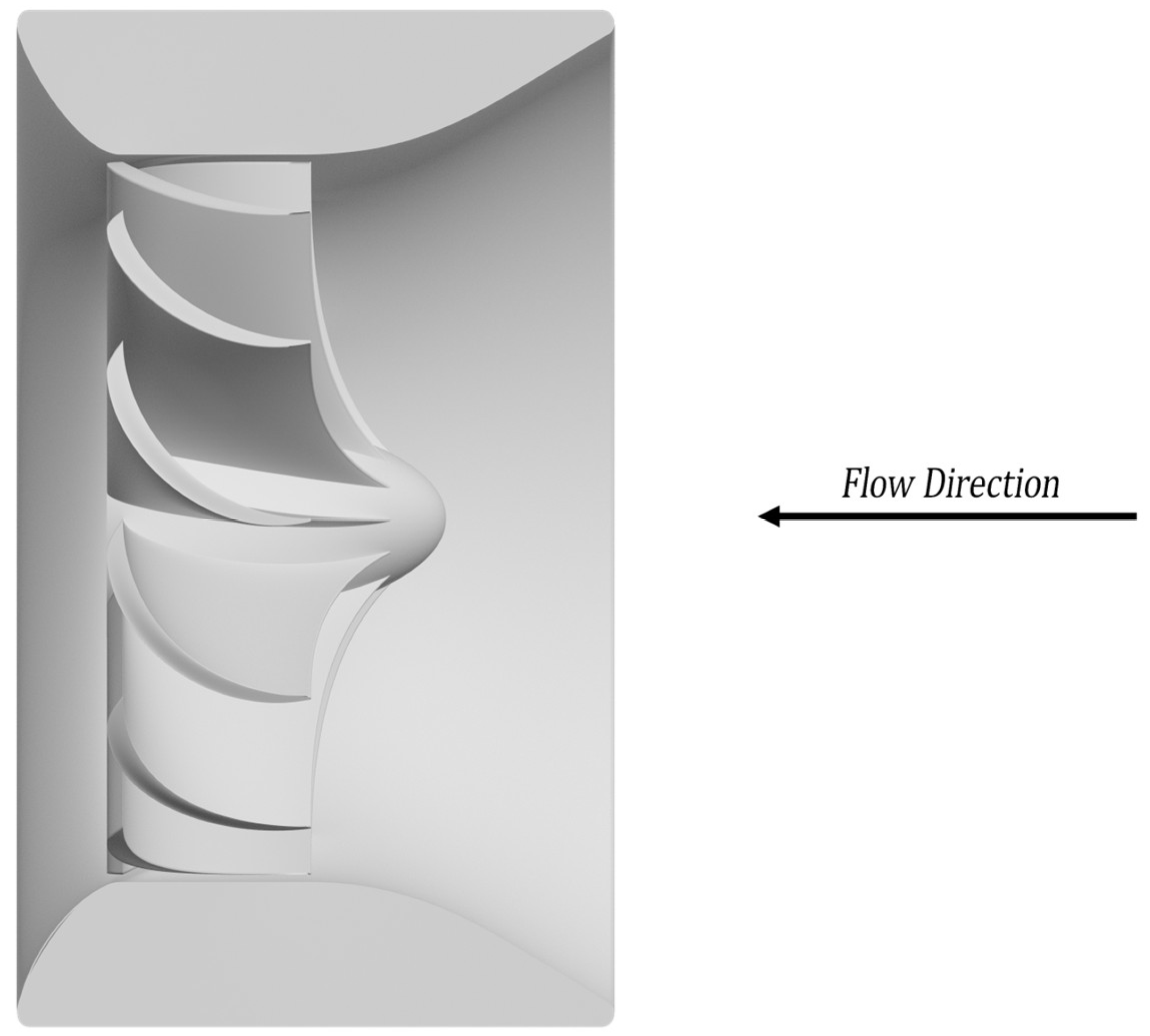
Figure 2.
(a) Axial view of a single blade attached to the rotor hub, observed along the z-axis, showing the radial projection of the blade and indicating the sectional plane A–B, which is detailed in Figure 3 to illustrate the elliptical projection of the flow deflection along the blade trajectory; (b) View obtained by rotating configuration (a) by 90° around the y-axis, highlighting the blade’s longitudinal curvature and the continuous angular deflection along its length; (c) View obtained by rotating configuration (b) by 90° around the x-axis, revealing a new three-dimensional perspective of the blade and rotor hub.
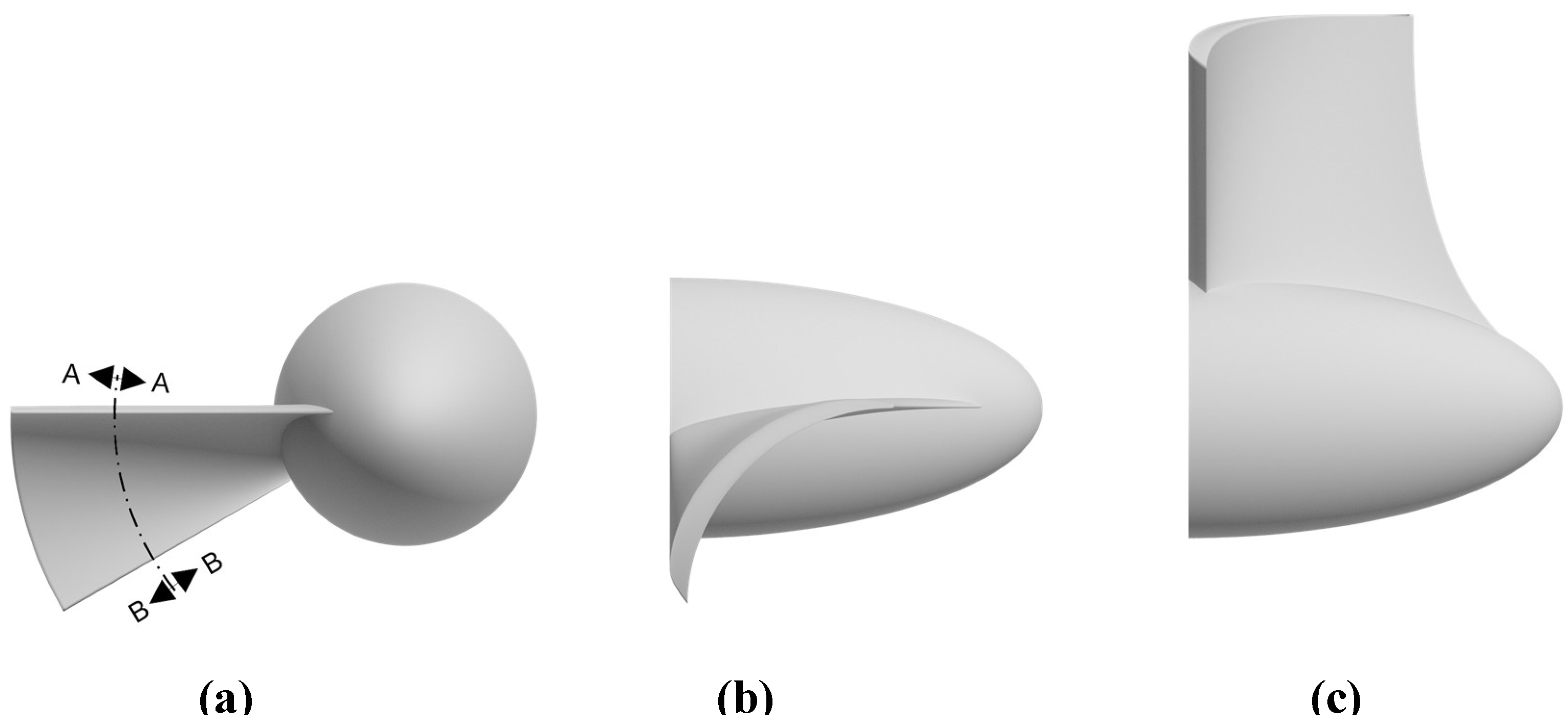
Figure 3.
Unfolded profile of the elliptical curvature of the blades, configured similarly across all radial positions of the rotor. The image represents the sectional cut indicated in Figure 2(a), on the A–B plane. In this configuration, the radius, , increases radially until it equals , defining the angular deflection. The projection of on the plane of Figure 2(a) corresponds to an arc of a circle, the length of which is determined by dividing the circumference by the total number of blades.
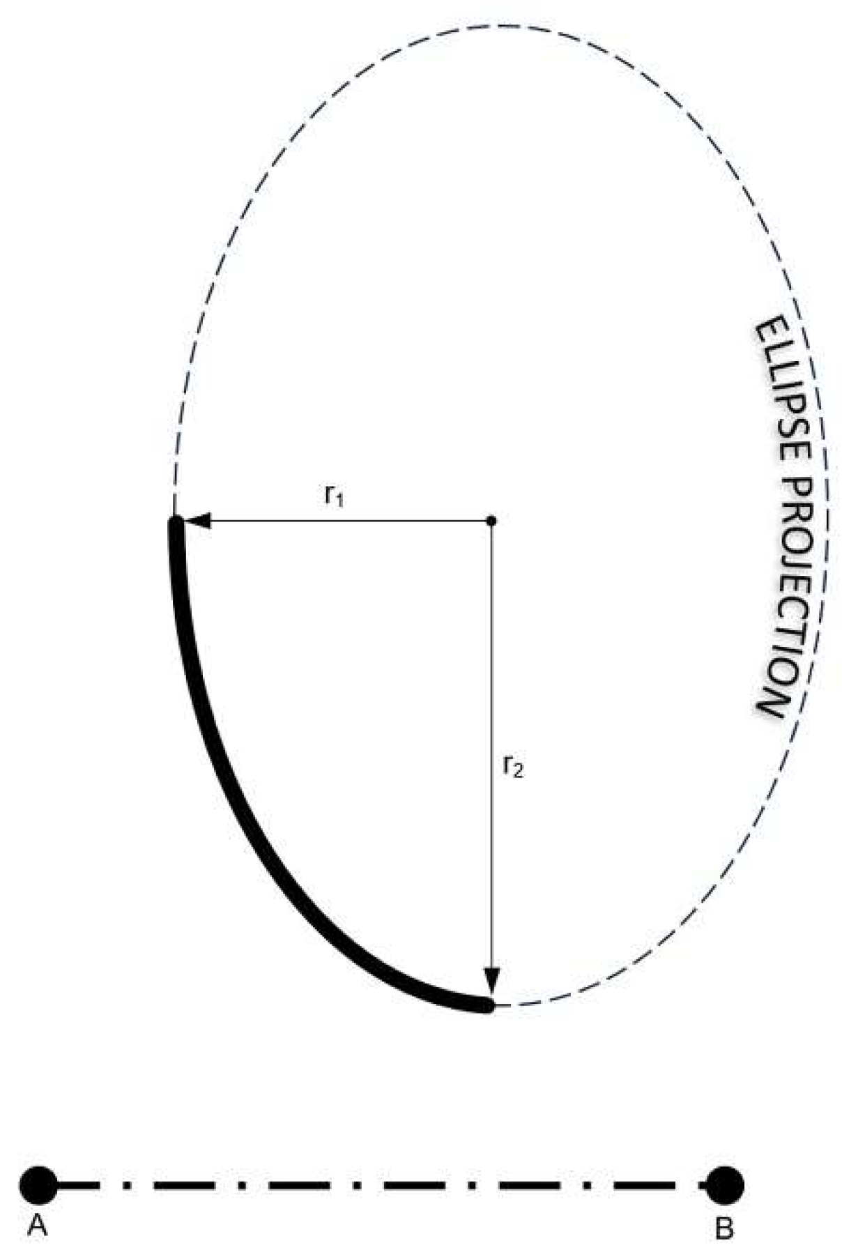
Figure 4.
Schematic illustration of the momentum vector deflection over the blade surface, indicating the progressive reorientation of the flow and the resulting tangential force.
Figure 4.
Schematic illustration of the momentum vector deflection over the blade surface, indicating the progressive reorientation of the flow and the resulting tangential force.
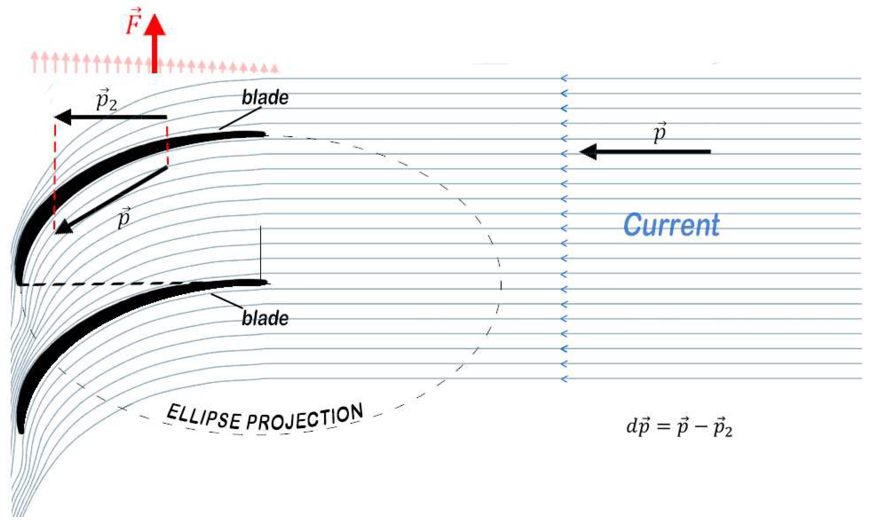
Figure 5.
Rotor geometry: (a) axial view (central projection) showing full occupation of the cross-sectional area by the blades, enabling complete interaction with the flow; (b) representation of the absence of bypass zones, illustrated by the continuous shadow produced by parallel light rays (representing idealised streamlines) incident on the rotor.
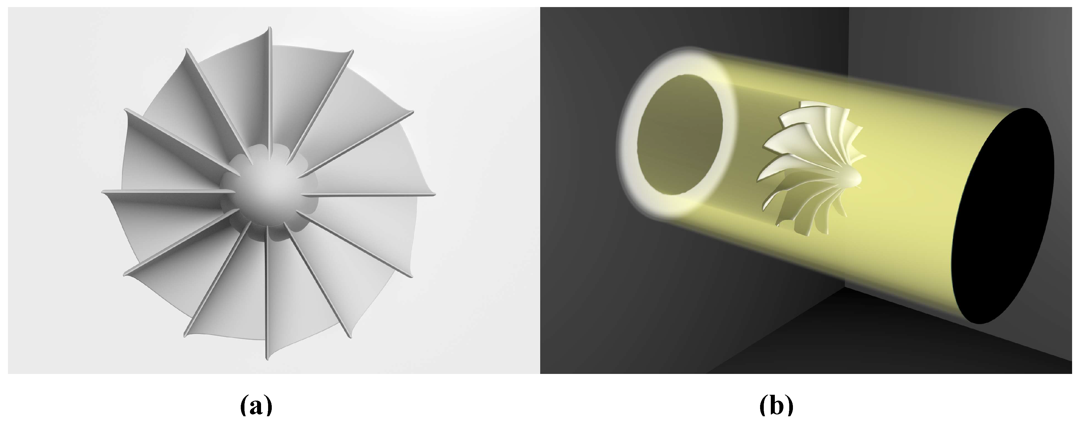
Figure 6.
Conceptual representation of the upstream control volume engaged by the hydrodynamic interaction with the ideal turbine. The extended region illustrates the volumetric coupling mechanism, highlighting the propagation of flow perturbation beyond the physical limits of the rotor.
Figure 6.
Conceptual representation of the upstream control volume engaged by the hydrodynamic interaction with the ideal turbine. The extended region illustrates the volumetric coupling mechanism, highlighting the propagation of flow perturbation beyond the physical limits of the rotor.
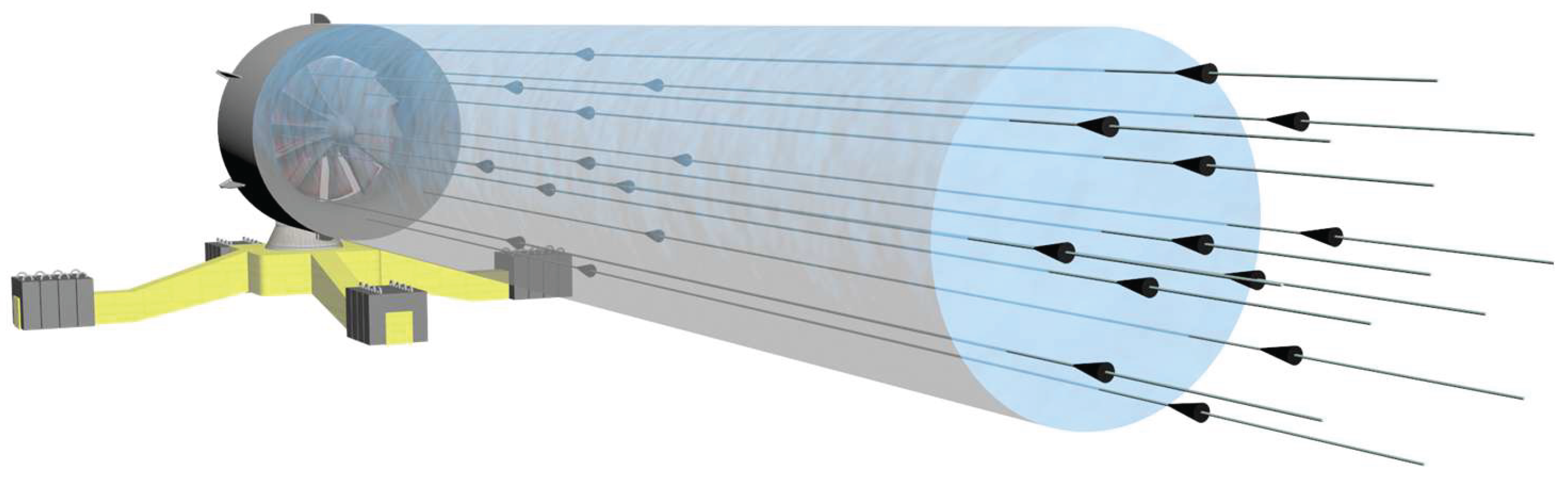

Table 1.
Key Differences Between Classical and Volumetric Ocean Energy Models
| Characteristic | Conventional Models (Wind/Submerged) | Volumetric Coupling Model with ERGF Framework (Ideal Turbine) |
|---|---|---|
| Operating Medium | Air (compressible) / Water (treated as partially incompressible) |
Ocean and river water (incompressibility assumed in modelling) |
| Energy Extraction Mechanism | Local axial flow deceleration | Vectorial redirection of linear momentum via angular deflection |
| Theoretical Efficiency Limit | ≤ 59.3% (Betz Limit) | Potentially higher; bounded by volumetric efficiency and physical limits |
| Energy Input Source | Not considered (finite incident energy) |
Assumed continuous via geophysical fields acting on large-scale water volumes |
| Flow Disturbance Profile | High turbulence and velocity gradients due to wake expansion |
Low turbulence; confined deflection without significant external disturbance |
| Cross-Sectional Flow Capture | Partial occupation with bypass zones |
Full capture through vectorial deflection (no bypass zones) |
| Spatial Interaction Scale | Confined to the rotor’s immediate swept area |
Extended volumetric coupling beyond rotor boundaries |
| Ecological Integration | Collision risk with fauna due to blade attack angle |
Low collision risk with fauna; smooth and gradual deflection |
| Design Philosophy | Wind turbine adapted to water | Tailored for incompressible media |
Disclaimer/Publisher’s Note: The statements, opinions and data contained in all publications are solely those of the individual author(s) and contributor(s) and not of MDPI and/or the editor(s). MDPI and/or the editor(s) disclaim responsibility for any injury to people or property resulting from any ideas, methods, instructions or products referred to in the content. |
© 2025 by the authors. Licensee MDPI, Basel, Switzerland. This article is an open access article distributed under the terms and conditions of the Creative Commons Attribution (CC BY) license (http://creativecommons.org/licenses/by/4.0/).
Copyright: This open access article is published under a Creative Commons CC BY 4.0 license, which permit the free download, distribution, and reuse, provided that the author and preprint are cited in any reuse.


