Submitted:
27 April 2025
Posted:
29 April 2025
You are already at the latest version
Abstract
In recent years, defect detection based on ultrasound B-scan images has been widely utilized in industry to detect the quality and presence of defects in products. However, there are still some difficulties in the process of processing B-scan images, such as sampling noise, huge amount of data and so on. In this paper, we analyse the acoustic characteristics of ultrasound B-scan image time series, design an image preprocessing method to make the image information gray-scale lossless, and propose a screening method for ultrasound B-scan image segments containing defects based on the theory of image entropy and recurrence diagram. Comparison experiments between this method and the traditional image entropy screening algorithm show that this method can solve the above difficulties to a certain extent and has its own superiority. The method proposed in this paper provides a new idea for processing ultrasound B-scan image sequences, and presents a new choice when the traditional method is in limitation.
Keywords:
ultrasound detection
; ultrasound B-scan
; deep learning
; image processing
; image entropy
1. Introduction
Currently, defect identification based on ultrasonic B-scan pictures constitutes one of the research hotpots in phased array ultrasonic testing (PAUT) technology. PAUT allows the collection of high-resolution B-scan pictures with greater sensitivity and clarity, displaying tremendous application potential in the examination of heterogeneous media and their contents.
In the use of ultrasonic B-scan, Wu Yuanming [1] adapted B-scan to the fault detection of railway freight vehicle wheelsets, considerably enhancing detection efficiency and accuracy. Luo Gengsheng [2] et al. suggested an ultrasonic guided wave detection technique based on B-scan imaging for identifying faults in oil and gas butt-welded elbows with anti-corrosion coatings. F. Honarva [3] et al. examined in depth ultrasonic testing techniques and their applications in damage detection of additive manufacturing items. Yuan Alin [4] et al. did experimental study on electromagnetic ultrasonic guided wave B-scan detection of fractures in aluminum sheets, carrying out studies on electromagnetic ultrasonic testing of aluminum sheet specimens with cracks. Zhang Wenxue [5] suggested a three-dimensional reconstruction analysis technique for metal cylinders based on ultrasonic testing. This approach includes rearranging pixel points using B-scan photography and then applying volume rendering methods for three-dimensional reconstruction analysis. In the realm of ultrasonic B-scan image detection, Gao Shuangsheng et al. [6] applied a morphological technique based on area reconstruction to segment fault features in ultrasonic images of brazed joints of guide rings and built related software using Matlab. Guo Beitao et al. [7] suggested an enhanced region expanding method to solve the issue of decreasing accuracy in defect detection of metal components in ultrasonic imaging pictures due to variables such as noise. Li Hua et al. [8], after using classical filtering algorithms to reduce noise in ultrasonic B-scan images of metal plates, compared the effects of three different image segmentation techniques and ultimately chose an improved seed region growing algorithm for accurate segmentation, which effectively highlighted defect features. Hu [9] et al. developed a deep learning-based hierarchical classification model to assess ultrasonic B-scan pictures of railway problems, utilizing a two-stage approach: model A for fuzzy classification and EfficientNet-B7 for fine-grained classification. Ye [10] et al. created a deep learning system named DPLA-Net (Dual Path Lesion Attention Network) for diagnosing different eye illnesses and normal eyes based on ocular B-scan pictures. Feng Wei [11] suggested a deep learning-based technique for defect recognition in ultrasonic B-scan pictures, performing experimental research on defect identification utilizing B-scan images produced by linear array phased array ultrasonic testing.
However, in the process of utilizing ultrasonic phased array technology to find faults in the industrial sphere, various issues are faced when dealing with ultrasonic B-scan pictures including defects. Firstly, directly captured B-scan pictures are typically affected with by numerous sorts of noise. This noise not only obscures the problem characteristics in the picture but also provides obstacles to human or automated defect identification, lowering the accuracy and reliability of defect detection. Secondly, B-scan pictures are often given in color format (three-dimensional data volume of R, G, and B values), and their enormous data volume greatly decreases the running performance of fault identification algorithms.
In response to these two issues, this study provides a screening approach for ultrasonic B-scan pictures including defects based on image entropy recurrence plots (hereafter referred to as the "recurrence method"). By comparing it with other screening techniques for ultrasonic B-scan image segments having flaws based on image entropy, the usefulness and superiority of this approach are established.
2. Materials and Methods
2.1. Image Features and Basic Concepts
2.1.1. Basic structural Properties of B-Mode Ultrasound Scan Pictures
Figure 1 depicts a schematic illustration of the key structural properties of a typical phased array ultrasonic B-scan picture. The picture is formed of a white-blue-yellow-red color gradient corresponding to echo strength from weak to strong, with each pixel reflecting the echo intensity at its corresponding position. A schematic illustration of the main structural properties of a typical phased array ultrasonic B-scan picture is presented in Figure 1.
When viewing the geographical composition of the picture, it is basically formed of four components from top to bottom: the surface echo zone, the dead zone, the backscatter zone, and the bottom echo zone. Among them, the backscatter zone corresponds to the ultrasonic echoes reflected within the workpiece under test. This section of the signal may be utilized to disclose the interior structural properties of the workpiece under test. The image qualities of this zone rely on the regularity of the workpiece and the existence of internal flaws, etc. Therefore, the picture properties of the backscatter zone constitute a significant foundation for defect identification and analysis. At the same time, typical defects exist in the form of a red core area wrapped by a yellow contour as shown in the figure; the bottom echo zone corresponds to the ultrasonic reflection signal that penetrates the workpiece and reaches the bottom surface of the workpiece, also known as the "bottom wave zone". It is characterized by a tiny region, continuous, and high-intensity red reflection echoes that span the whole width of the picture, frequently accompanied by a thin yellow band surrounding it. The bottom echo zone is the border of an ultrasonic testing process, and its location may disclose the thickness of the workpiece, and its morphology can reflect the bottom structure of the workpiece to a certain degree.
2.1.2. Image Entropy
Entropy is a physical number that defines the degree of disorder in a system in the area of physics, and in information theory, it is used to characterize the amount of information contained in a specific signal. As a two-dimensional carrier for storing information, pictures have a greater data density than one-dimensional signals, and consequently have a corresponding entropy value that reflects the amount of information they carry - image entropy. picture entropy is a statistical kind of feature that displays the average amount of information in a picture and represents the aggregation properties of the grayscale distribution of the image. According to the notion of entropy in information theory, from the standpoint of the distribution of grayscale values in a grayscale picture, it is a practical way to exploit the aggregation features of grayscale distribution to represent the amount of information contained in the image. Let be the weight of pixels with grayscale value among all pixels, then the unary grayscale entropy of the grayscale picture is:
Through equation (1), the grayscale information of each pixel in a B-scan picture may be turned into image entropy information for the whole image, enabling data compression. The image entropy sequence of a series of B-scan picture sequences is presented in Figure 2.
2.1.3. Phase Space Reconstruction
For a non-stationary deterministic system, its characteristics are frequently explored in a high-dimensional phase space. The objective of phase space reconstruction is to try to mine additional information from the complete time series and locate another new system equal to the original system in high dimensions.
In 1980, Packard [12] and other researchers presented a technique for reconstructing the phase space of a one-dimensional time series, known as the coordinate delay reconstruction method or the time delay reconstruction method. The crux of this strategy rests in leveraging data from various time points in the time series to generate an m-dimensional phase space vector by imposing a time delay. Subsequently, in 1981, Taken [13] presented an important theorem, the "embedding theorem". The theorem states that for a one-dimensional scalar time series of an infinitely long and undisturbed m-dimensional dynamic system, one can always find an embedded phase space of at least m dimensions such that this phase space remains topologically consistent with the original system, provided that satisfies . Based on the embedding theorem, an image entropy high-dimensional phase space may be generated from the image entropy sequence, and further tasks such as state determination and feature analysis of the image entropy sequence are carried out based on the reconstructed image entropy phase space.
The following are the particular stages of phase space reconstruction: (1) Obtain a one-dimensional scalar time series;(2) Determine the delay time and the embedding dimension ; (3) Construct a (n-(m-1)τ)×m dimensional reconstructed vector X(t_i), where each row vector is derived using equation (10):
As can be observed from the creation processes of the vector, there are two basic parameters: the embedding dimension and the time delay . However, the embedding theorem does not give exact methods for computing these two values. In real applications, as time series data frequently includes noise and has limited length, the values of these two parameters need to be determined depending on the unique scenario.
2.1.4. Recurrence Plot Method
After rebuilding the phase space of a one-dimensional image entropy sequence, we receive a mapping space consisting of N m-dimensional (embedding dimension) vectors, which may then be examined using recurrence plots. A recurrence plot (Recurrence Plot, RP) is basically a technique for visualizing phase spaces of various dimensions inside a two-dimensional space. It calculates the Euclidean distance matrix of the phase space state vectors by determining the distance between two separate state vectors and , as illustrated in equation (16):
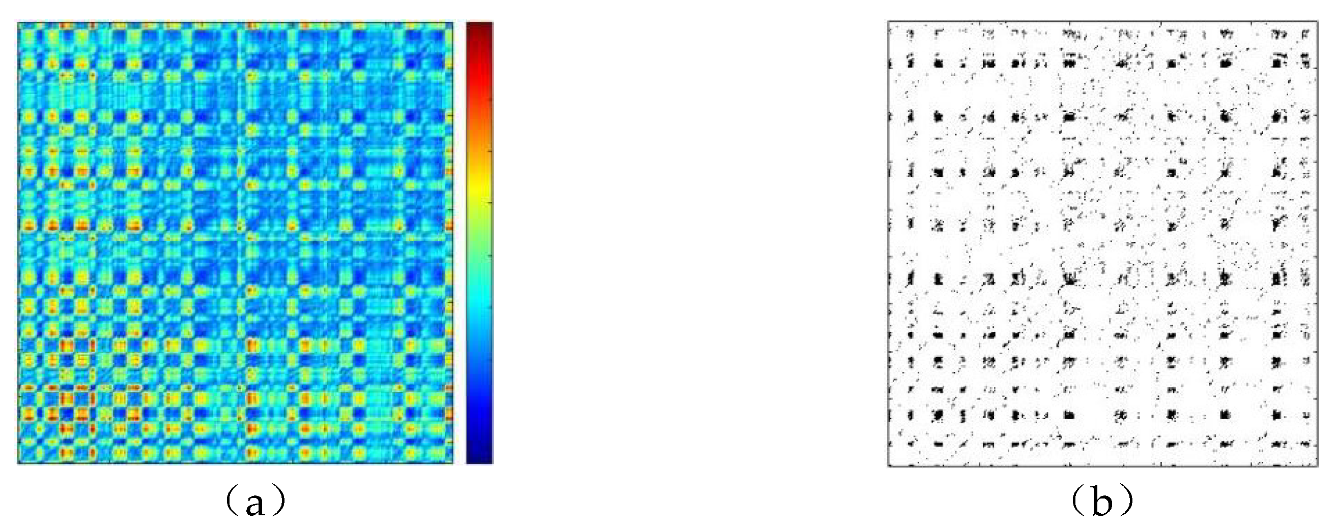
where represents the distance between two vectors; It can be observed that the procedure provides a matrix for any dimensional phase space. By coloring depending on the highest and lowest values in the matrix, a color map indicating the distance distribution of the matrix components may be generated. Blue is often used to signify proximity, and red to represent distance. Such a picture is also termed a threshold-free recurrence plot. The threshold-free recurrence plot following phase space reconstruction of the sampled signal sequence with and is presented in Figure 3.
Through the threshold-free recurrence plot, it is feasible to examine and evaluate rebuilt phase spaces of any dimension at a two-dimensional level. However, owing to concerns such as substantial discrepancies in the absolute values of components, it is difficult to examine threshold-free recurrence plots of various kinds of signals using invariant criteria. Therefore, relevant researchers have developed a binary recurrence plot presentation approach, defining the phase point-threshold distance matrix as follows:
In the formula, ε is a manually chosen threshold used to compare the values in the distance matrix , and .
The phase point-threshold distance matrix generated by the foregoing computation is a square matrix, and its members only contain 0 and 1. Starting from such a matrix , assign black to points having an element value of 1 and white to points with an element value of 0. The produced binary picture is termed a "binary recurrence plot".
2.2. Method Design
2.2.1. Overall Technical Route
The technical way of the recurrence technique is as follows: First, preprocess the B-scan pictures, then calculate the image entropy of the preprocessed B-scan image sequence to produce the image entropy sequence. On this basis, execute phase space reconstruction to produce the binary recurrence plot of the image entropy sequence. Then, utilize the fraction of recurrence points in the recurrence plot space to characterize the likelihood of numerical mutations in the picture entropy owing to defect features, and generate a filter used to screen suspected faulty sequences. Finally, forecast the distribution of suspected faulty picture sequences using the filtered image entropy sequence. The technical way of the recurrence technique is depicted in Figure 5.
2.2.2. Image Preprocessing
In order to accomplish standardization and normalizing of picture representation for B-scan images, it is required to preprocess the original images at the beginning. The preparation procedure is presented in Figure 6.
To reduce information loss during the grayscale conversion of B-scan color pictures, this work offers an information-lossless full-mapping grayscale conversion technique. The algorithm for calculating grayscale values from RGB values is presented in Equation (5):
Secondly, via experiments, median filtering was shown to reduce noise in grayscale pictures to the maximum degree, while the opening operation displayed the largest enhancing impact on defect edge characteristics in images. This study employs median filtering as the smoothing and denoising approach, and the opening operation as the morphological processing method.
ROI refers to the "Region of Interest", which is the key region of a picture for attaining the intended purpose. It frequently includes critical information that needs identification, analysis, and processing. By studying photos after grayscale conversion, smoothing/denoising, and morphological processing, it was observed that their row grayscale mean values display characteristics of changing gradually from top to bottom with regional variations. Calculating their row grayscale mean curves showed that for each B-scan picture, the top of the surface echo and the bottom of the bottom echo correspond to the places where the row grayscale mean value first considerably rises and last dramatically declines, respectively. By choosing suitable thresholds based on these parameters, ROI extraction of B-scan pictures may be achieved. The row grayscale mean curve of the picture is displayed in Figure 7:
2.2.3. Phase Space Reconstruction Optimal Delay Time and Embedding Dimension Selection
According to the embedding theorem described in Section 1.2, given an indefinitely long noise-free time series, the delay time may be freely set. However, significant practical research have revealed that phase space representation is strongly reliant on the selection of τ. The main idea is to guarantee reconstructed vectors are as mutually independent as feasible.
This work applies the mutual information approach to estimate the best delay time τ. The mutual information coefficient (MI) is used to measure the correlation strength between state vectors following phase space reconstruction. Based on the aforementioned examination of recurrence plot theory, it can be determined that a lower mutual information coefficient implies poorer connection between state vectors, which better reveals rapid changes in system patterns.
The average information content of the system about the sum of variables is defined as the system's information entropy, called joint entropy. Its calculating formula is presented in Equation (6):
The spatial mutual information coefficient may be calculated as illustrated in Equation (7):
At this point, the delay time corresponding to the initial local minimum value of the mutual information coefficient is chosen as the ideal delay time for phase space reconstruction of the image entropy sequence in this segment.
The purpose of selecting an appropriate embedding dimension m is to fully unfold the geometric structure of the attractor as much as possible, thereby characterizing the system's attractor without losing information carried by the original image entropy sequence and revealing the characteristics of the system under analysis. If the embedding dimension m is too small, the attractor will overlap, allowing phase space points from various trajectories to appear in the same neighborhood. This leads in a substantial gap between the reconstructed attractor and the system's true attractor, reducing the accuracy of subsequent quantitative evaluations. Conversely, if m is too big, while guaranteeing the attractor's geometric structure is completely unfurled, it also amplifies noise and increases computing complexity.
This study adopts the enhanced False closest Neighbors (FNN) approach described by Cao's algorithm [14], which provides a distance coefficient based on the notion of false closest neighbors:
Define the metric (average rate of change of Euclidean distances between phase points induced by dimensionality increase) :
Using the rate of change ratio of the metric value as the requirement for the minimal embedding dimension:
At this point, examine the trend of as m varies, and pick the embedding dimension corresponding to the place where starts to converge to 1 as the minimal phase space reconstruction embedding dimension for this image entropy sequence.
2.2.4. binarization recurrence plot threshold selection
According to the definition of the binarized recurrence plot, it contains the following characteristics:
The primary diagonal values of the square matrix are always 1.
The square matrix is symmetrical along the diagonal (Line of identity, LOI).
For a binarized recurrence plot of a specific signal sequence, the choice of threshold is critical, since it impacts the final appearance of the binarized recurrence plot. The selection of thresholds considerably changes the display of the binarized recurrence plot and, additionally, affects the analysis and identification of its system properties. When the threshold value is too little, the number of recurrence points in the recurrence plot is inadequate, which cannot properly describe the system's features. Conversely, when the threshold value is too big, a large number of recurrence points will show as continuous block-like black regions in the recurrence plot, masking valuable recurring feature information. The binarized recurrence graphs under various thresholds are given in Figure 8.
As can be seen from the locally expanded partial details of the binarized recurrence plot in Figure 8, when the threshold is set to 5% of the recurrence points percentage, the binarized recurrence plot reveals unique local diagonal characteristics and white crosshair features. At this stage, the pattern changes in the B-scan image sequence may be most clearly portrayed, and it can be determined if the binarized recurrence plot of the sample sequence adheres to the macroscopic structural properties of recurrence plots in abrupt change modes. It is determined that there is an abrupt shift in the system state of this picture entropy series.
2.2.5. Faulty Image Screening Filter Design
By evaluating the features and defects of the binarized recurrence plot, it can be shown that the emergence of local diagonal features and white crosshair lines typically correlates to rapid changes in image entropy induced by defects. The existence and distribution of faults alter the distribution of recurrence spots in the recurrence plot. The more the white crosshair lines are spread, the more important the changes in the picture entropy sequence at the relevant time compared to the image entropy sequence at consecutive times.
Based on the foregoing analysis, a filter for the image entropy sequence may be created by merging the distribution density function of recurrence points along the time series in the binarized recurrence plot. This filter improves the image entropy intervals suspected of having defect features while weakening those that do not, in order to assist the screening of B-scan pictures suspected of containing flaws.
Assuming that the original picture entropy sequence comprises sample points, the size of the recurrence plot is determined as follows:
For the -th row or column in the recurrence plot, it shows if the phase distance reconstructed between the -th instant and other moments passes the threshold. This also depicts, to a certain degree, the chance of a pattern mutation happening at the -th instant compared to other times. In this respect, paired with the diagonally symmetric qualities of the recurrence plot, the distribution density of recurrence points in rows or columns may be utilized to quantify the probability density of pattern modifications.
The vector formed of is the filter to be solved.
To standardize the numerical range of the filter, each in is normalized.
At this point, the numerically normalized filter is obtained.
Multiply the amplitude values of the example image entropy sequence at each time point by the normalized distribution density coefficients of the filter at each time point to produce, which is the primary non-systematic abrupt change component of the image entropy sequence. The amplitude value at a specific time point is .
On this premise, the difference between and may be used to identify the variation in image entropy produced by system mutations (which can be defined as the variation caused by "defect characteristics + environmental interference") , and the amplitude at a specific point :
The normalized filter is displayed in Figure 9, the filtered image entropy sequence is given in Figure 10, and the image entropy variation sequence )is presented in Figure 11.
In Figures 9, 10, and 11, green and red vertical dashed lines are utilized to represent the sequence intervals of pictures with genuine fault features. It can be observed that the non-zero weight areas of the normalized filter nearly totally encompass the real fault intervals. At the same time, the positive areas of image entropy and image entropy variation after filtering likewise almost totally encompass the real fault intervals. Considering that the image entropy variation sequence most directly represents the system mutation induced by defect features, the B-scan pictures with image entropy variation larger than 0 are regarded as suspected defective images, therefore accomplishing the screening of suspected defective images.
3. Results
To verify the application effect of the above recursive-based screening method for defective B-scan image sequences in actual production scenarios, this paper selects a set of long-sequence image entropy data with 4752 B-scan images, hereinafter referred to as the "experimental sequence", for experimentation. The experimental findings are contrasted with those of two classic screening approaches, the threshold method and the sliding window method. The pre-processed pictures and image entropy sequences of the experimental sequence are displayed in Figure 12 and Figure 13, respectively.
Based on the experimental sequence, phase space reconstruction was done with the optimum delay time and embedding dimension . On this basis, a threshold-free recurrence plot illustrated in Figure 14(a) was developed. Then, a binarized recurrence plot depicted in Figure 14(b) was constructed by choosing an acceptable recurrence point ratio of 5%. Finally, the normalized filter function shown in Figure 14(c) was calculated according to the steps described in Section 2.5, and the filtered image entropy sequence shown in Figure 14(d), the image entropy variation sequence shown in Figure 14(e), and the defect distribution interval shown in Figure 14(f) were obtained.
Apply the threshold technique and sliding window method (with indicators set as mean, maximum, and variance values) to the experimental sequence. Define the efficacy assessment indicators as the filtering rate, interval coverage rate, and complete coverage rate. Their computation techniques are presented in equations (18) to (20). To guarantee that the screening results include the acoustic picture that best fits the defect, it is needed that sample points around the center of the defect interval must not be missing or discontinuous. In other words, only the suspected faulty intervals filtered out are permitted to have missing judgments at the beginning and end sections compared to the real defective intervals. By synthesizing the aforementioned three quantitative factors and one qualitative criterion, the impacts of various screening techniques can be objectively and fully analyzed, and the ideal approach may be chosen.

Table 1.
The assessment results of the three approaches are provided in Table 1.
Table 1.
The assessment results of the three approaches are provided in Table 1.
| Screen Method | Interval Condition | Comprehensive Condition | |||||||
|---|---|---|---|---|---|---|---|---|---|
| Defect Interval Length | 33 | 140 | 40 | 130 | 31 | 11 | |||
| Thresholding Method | Whether the central part is missed during inspection | no | no | yes | yes | yes | no | Filter Rate | 69% |
| coverage rate | 85% | 80% | 76% | 77% | 87% | 100% | Comprehensive Coverage Rate | 81% | |
| Averaging Method | Whether the central part is missed during inspection | no | no | no | no | no | no | Filter Rate | 60% |
| coverage rate | 89% | 82% | 91% | 89% | 100% | 100% | Comprehensive Coverage Rate | 90% | |
| Maximum Value Method | Whether the central part is missed during inspection | no | no | no | no | yes | no | Filter Rate | 61% |
| coverage rate | 89% | 82% | 91% | 83% | 89% | 67% | Comprehensive Coverage Rate | 85% | |
| Variance Method | Whether the central part is missed during inspection | no | yes | yes | yes | no | no | Filter Rate | 60% |
| coverage rate | 67% | 82% | 64% | 89% | 50% | 89% | Comprehensive Coverage Rate | 69% | |
| Recurrence Method | Whether the central part is missed during inspection | no | no | no | no | no | no | Filter Rate | 49% |
| coverage rate | 91% | 95% | 98% | 92% | 100% | 100% | Comprehensive Coverage Rate | 95% | |
The data with the greatest filtering rate, complete coverage rate, and single interval coverage rate are highlighted in bold. The findings demonstrate that the recursive technique has the best coverage rate in all defect intervals, as well as the most comprehensive coverage rate, and no center interval is missing. However, in terms of the filtering rate, the recursive technique performs significantly worse than the other methods, at roughly 50%.
Based on a complete examination of the experimental data, it can be stated that the recursive technique may produce the most reliable screening effect for faulty ultrasonic phased array B-scan pictures, with nearly ideal reliability.
4. Discussion
The suggested approach increases fault identification in ultrasonic B-scan pictures by integrating image entropy analysis with recurrence plots. Experimental findings indicate a 95% complete defect coverage rate, exceeding standard thresholding (81%) and sliding window approaches (85–90%). This derives from the recurrence plot’s sensitivity to entropy changes caused by flaws, assuring minimum crucial interval omissions. While the filtering rate (49%) needs further verification, this emphasizes reliability—crucial in industrial settings where defect supervision is pricier than human inspections.
Unlike deep learning algorithms needing considerable training data [9,10,11], this method changes parameters (e.g., delay time τ, embedding dimension m) dynamically to each sequence, boosting scalability. Preprocessing using median filtering and morphological processes also overcomes noise difficulties presented by prior approaches [6,7,8].
The method is especially interesting for evaluating heterogeneous materials (e.g., composites, additive-manufactured components), since grayscale entropy reduction decreases computing effort, allowing real-time application. Future work should investigate hybrid frameworks mixing recurrence-based screening with lightweight deep learning models to decrease false positives. Broader validation across fault kinds (micro-cracks, porosity) and materials (polymers, ceramics) would increase generalizability. Adaptive threshold selection for recurrence graphs and hardware acceleration might further enhance performance.
In summary, our technique blends classic image processing with current flexibility, delivering a robust, dataset-independent solution for industrial nondestructive testing. Continued enhancement via hybrid systems and broader validation will establish its practical value.
5. Conclusions
Through experimental results and combined with the implementation logic of the recursive method, it can be seen that compared with traditional screening methods that require a large number of experiments to determine certain parameters, the selection of parameters in the recursive method process only depends on each segment of the image entropy sequence itself. Whether it is the delay time and embedding size of phase space reconstruction, or the recursion point ratio of the binary recurrence plot, it is not required to refer to a large number of experimental data to rapidly and precisely pick approximately ideal values. This demonstrates that the recursive technique described in this study has a natural advantage in scalability compared with standard screening methods, and has strong scalability when confronting the job of screening faulty B-scan pictures of diverse kinds of work pieces.
Author Contributions
Conceptualization, P. C. and Q. L.; methodology, P. C.; software, P. C.; validation, P. C., Q. L., and B. T.; formal analysis, Q. L.; investigation, B. T.; resources, G. T.; data curation, G. T.; writing—original draft preparation, P. C.; writing—review and editing, C. Y.; visualization, P. C.; supervision, P. C.; project administration, P. C.; funding acquisition, C. Y. All authors have read and agreed to the published version of the manuscript.
Funding
This research was funded by: Major Special Projects of Shanxi Province, grant number 20201102003; Zhejiang Provincial Market Supervision and Administration Bureau,grant number ZD2024012; Zhejiang Provincial Natural Science Joint Fund Key Project, grant number LLSSZ24E050001.
Institutional Review Board Statement
Not applicable.
Informed Consent Statement
Not applicable.
Data Availability Statement
The original contributions presented in this study are included in the article. Further inquiries can be directed to the corresponding author.
Acknowledgments
This work was funded by Shanxi Province, Zhejiang Market Supervision Bureau, and Zhejiang Natural Science Joint Fund. We thank colleagues for technical and administrative support.
Conflicts of Interest
The authors declare no conflicts of interest.
References
- Wu, Y.M. B-scan Ultrasonic Imaging Testing Equipment and Its Application in Freight Axle Inspection. Railway Quality Control 2017, 45, 24–26. [Google Scholar]
- Luo, G.S.; Dai, X. Ultrasonic Guided Wave Testing for Defects in Oil-Gas Butt Welded Elbows Based on B-scan Imaging. Nondestructive Testing 2019, 41, 53–57. [Google Scholar]
- Honarvar, F.; Varvani-Farahani, A. A review of ultrasonic testing applications in additive manufacturing: Defect evaluation, material characterization, and process control. Ultrasonics 2020, 108, 106227. [Google Scholar] [CrossRef] [PubMed]
- Yuan, A.L.; Lai, Y.Q.; Shi, J.; Duan, J.F.; Lu, C.; Shi, W.Z. Experimental Study on Electromagnetic Ultrasonic Guided Wave B-scan Detection for Cracks in Aluminum Thin Plates. Technical Acoustics 2022, 41, 211–219. [Google Scholar]
- Zhang, W.X. Ultrasonic Testing and Reconstruction of Internal Defects in Metal Columns. Nondestructive Testing 2023, 45, 7–10. [Google Scholar]
- Gao, S.S.; Gang, T.; Chi, D.Z. Image Processing and Quality Evaluation of Ultrasonic Testing for Guided Ring Brazed Joints. Welding & Joining 2012, 23–25. [Google Scholar]
- Guo, B.T.; Ye, S.H.; Zhang, L.X. Defect Detection in Metal Ultrasonic Images Based on Region Growing. Modular Machine Tool & Automatic Manufacturing Technique 2023, 132–136. [Google Scholar]
- Li, H.; Zhu, B. Research on Image Processing for Metal Sheet Defects Based on Visualized Laser Ultrasonics. Industrial Control Computer 2023, 36, 89–91. [Google Scholar]
- Hu, G.; Li, J.; Jing, G. Rail Flaw B-Scan Image Analysis Using a Hierarchical Classification Model. International Journal of Steel Structures 2024, 1–13. [Google Scholar] [CrossRef]
- Ye, X.; He, S.; Dan, R. Ocular Disease Detection with Deep Learning (Fine-Grained Image Categorization) Applied to Ocular B-Scan Ultrasound Images. Ophthalmology and Therapy 2024, 13, 2645–2659. [Google Scholar] [CrossRef] [PubMed]
- Feng, W. Experimental Study on Defect Recognition in Ultrasonic B-scan Images Using Deep Learning. Nondestructive Inspection 2024, 48, 21–26. [Google Scholar]
- Packard, N.H.; Crutchfield, J.P.; Farmer, J.D.; Shaw, R.S. Geometry from a Time Series. Physical Review Letters 1980, 45, 712–716. [Google Scholar] [CrossRef]
- Takens, F. Detecting strange attractors in turbulence. Berlin, Heidelberg, 1981; pp. 366-381.
- Cao, L. Practical method for determining the minimum embedding dimension of a scalar time series. Physica D: Nonlinear Phenomena 1997, 110, 43–50. [Google Scholar] [CrossRef]
Figure 1.
Schematic illustration of essential structural properties of typical phased array ultrasonic B-scan image.
Figure 1.
Schematic illustration of essential structural properties of typical phased array ultrasonic B-scan image.
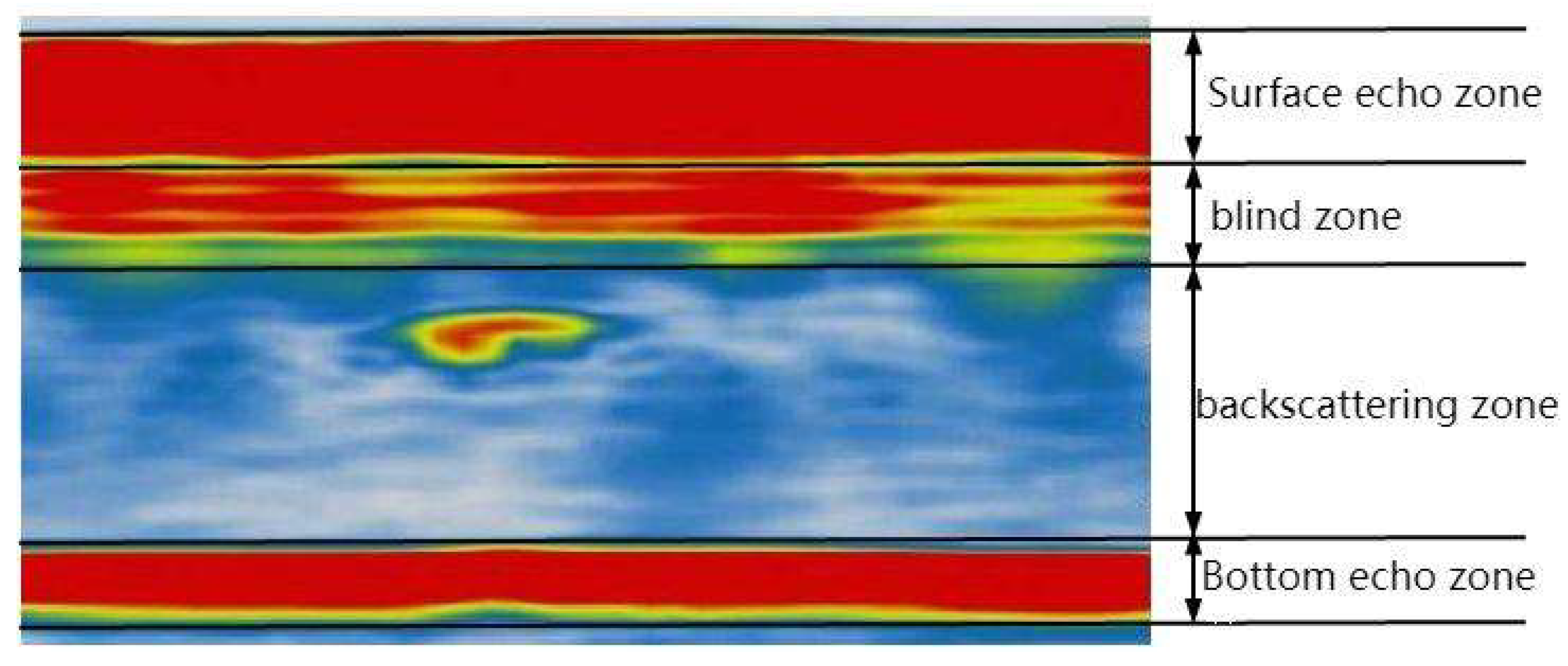
Figure 2.
Example sequence of image entropy.
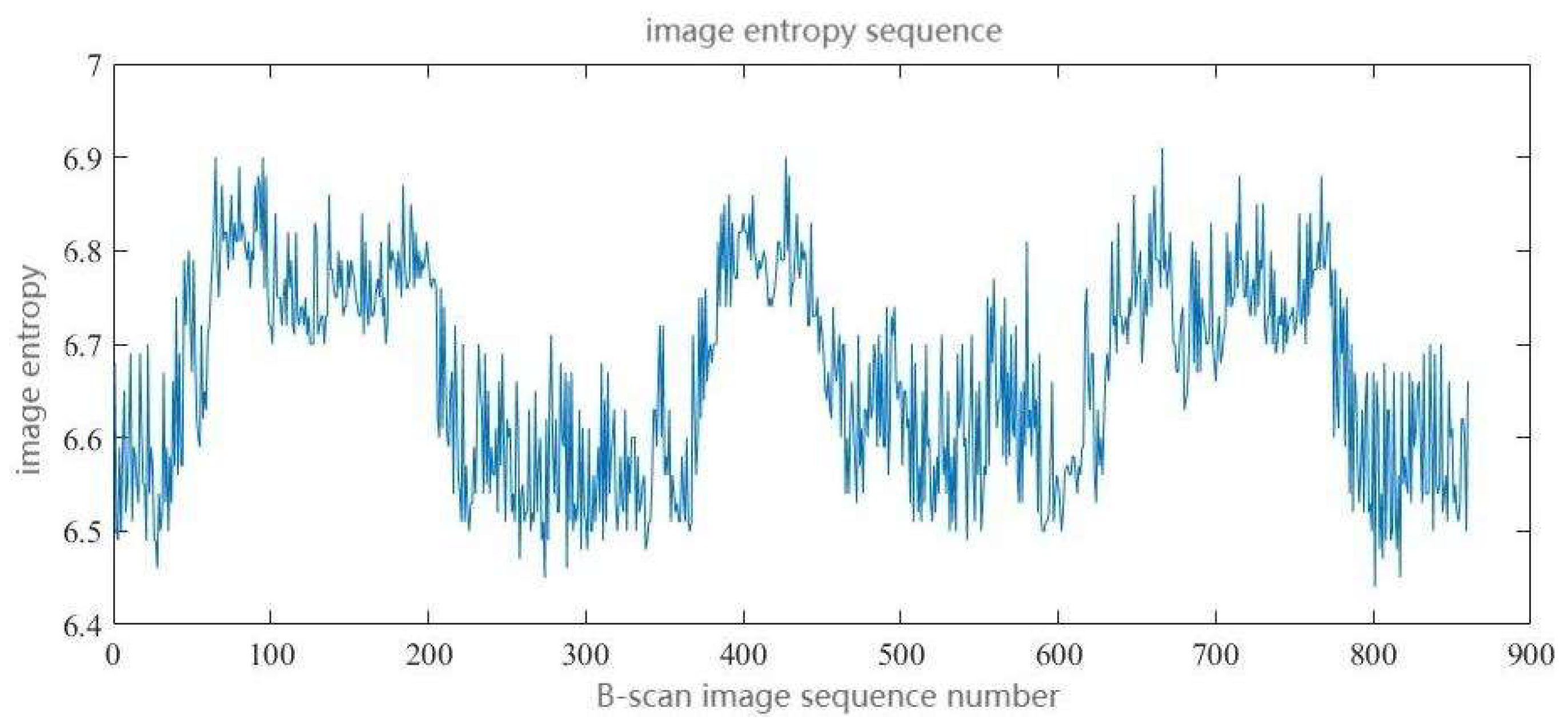
Figure 3.
Example of a threshold-free recurrence plot.
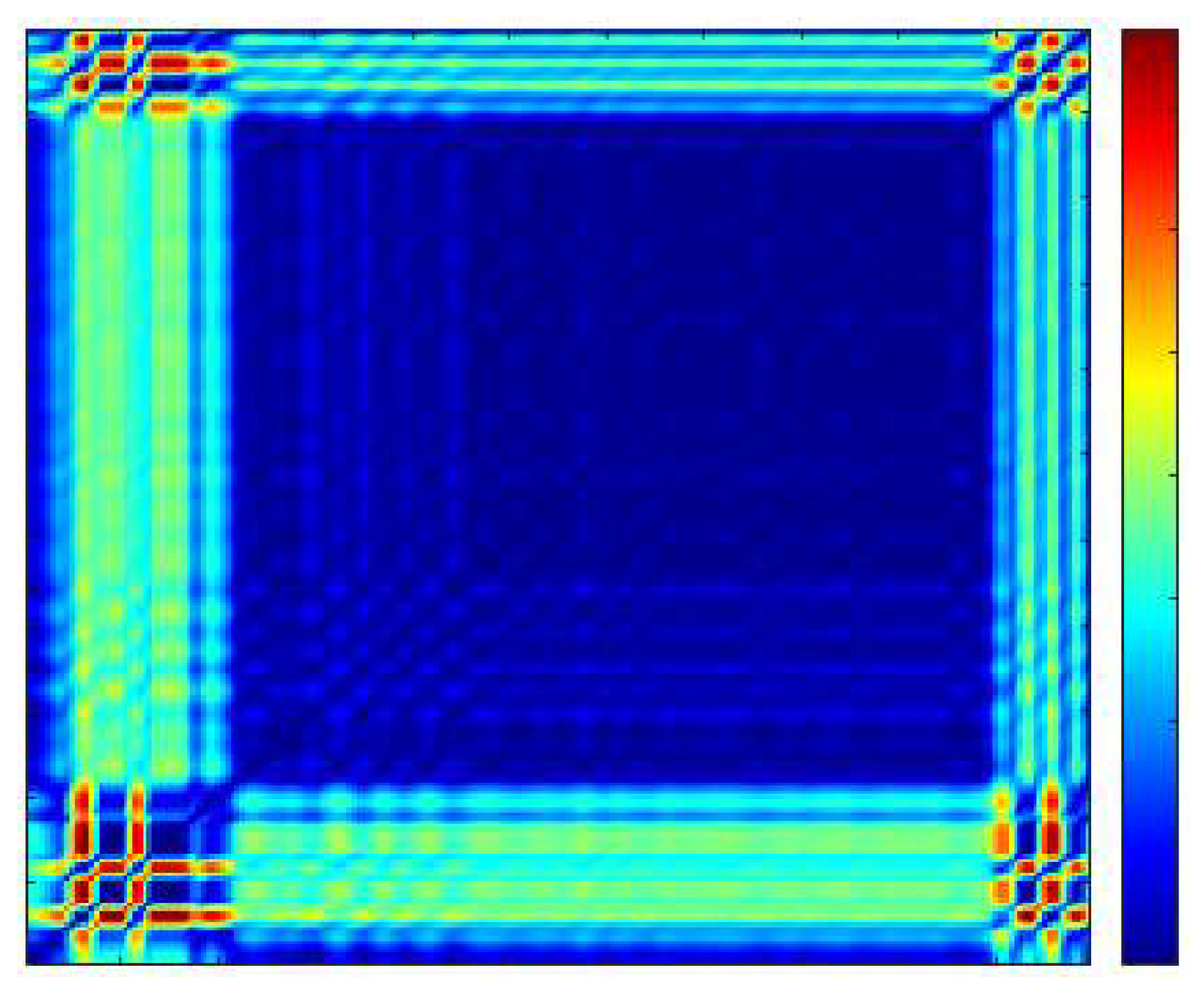
Figure 4.
Example of a binary recurrence plot.
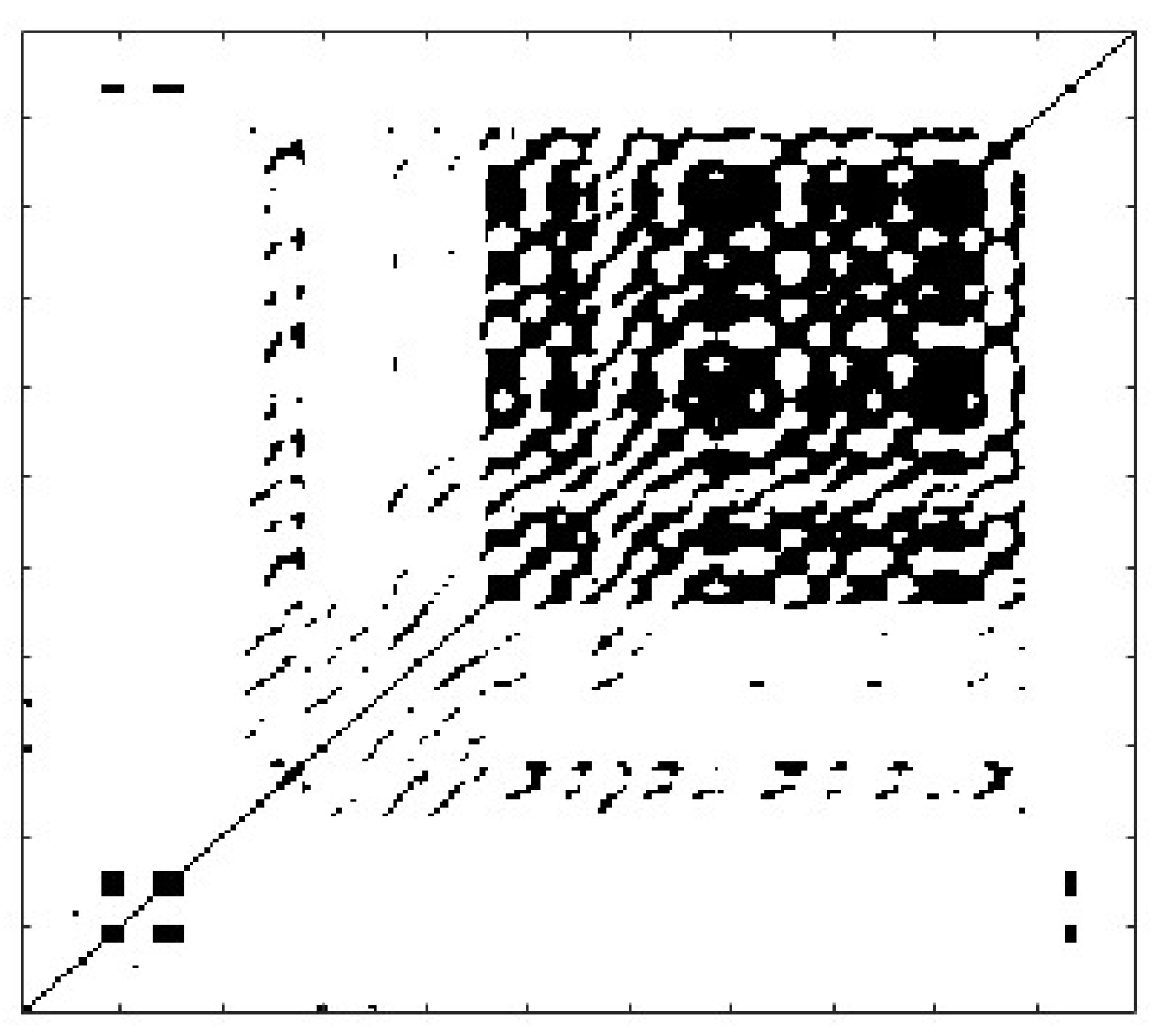
Figure 5.
Technical approach of the screening technique based on image entropy recurrence plot.
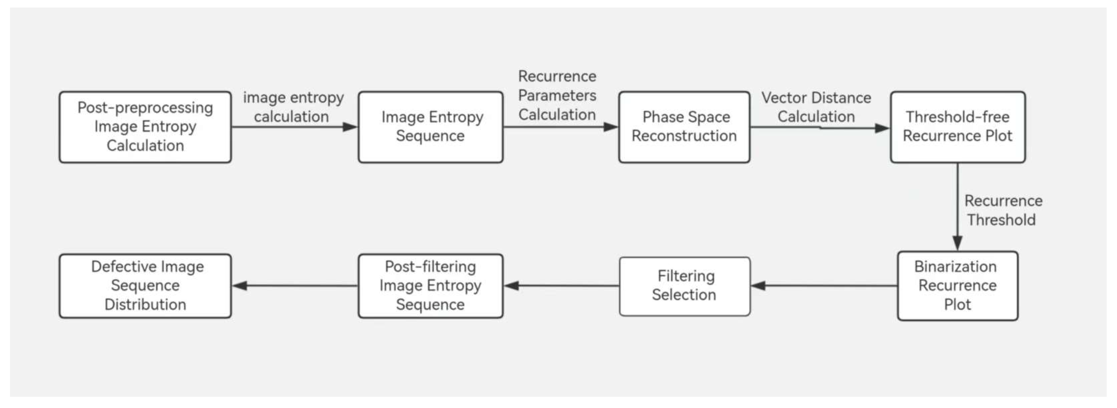
Figure 6.
B-scan Image Preprocessing Workflow.
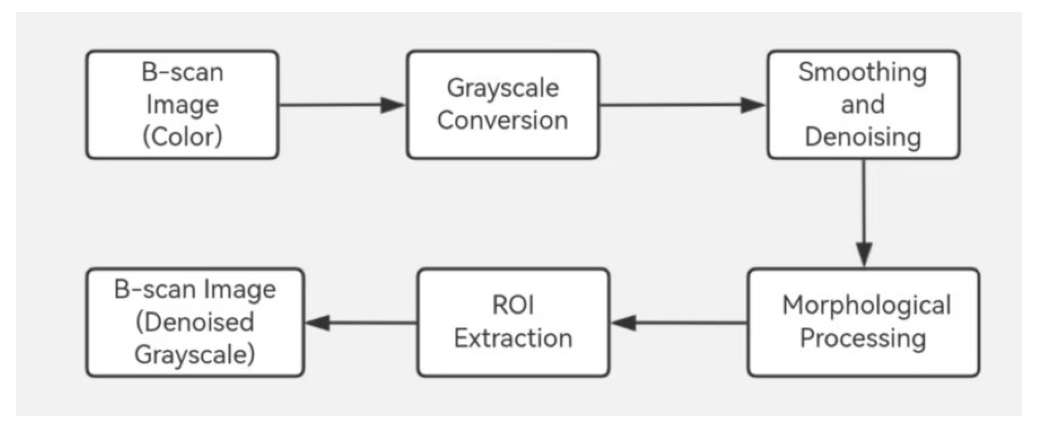
Figure 7.
Image and its row grayscale mean curve.
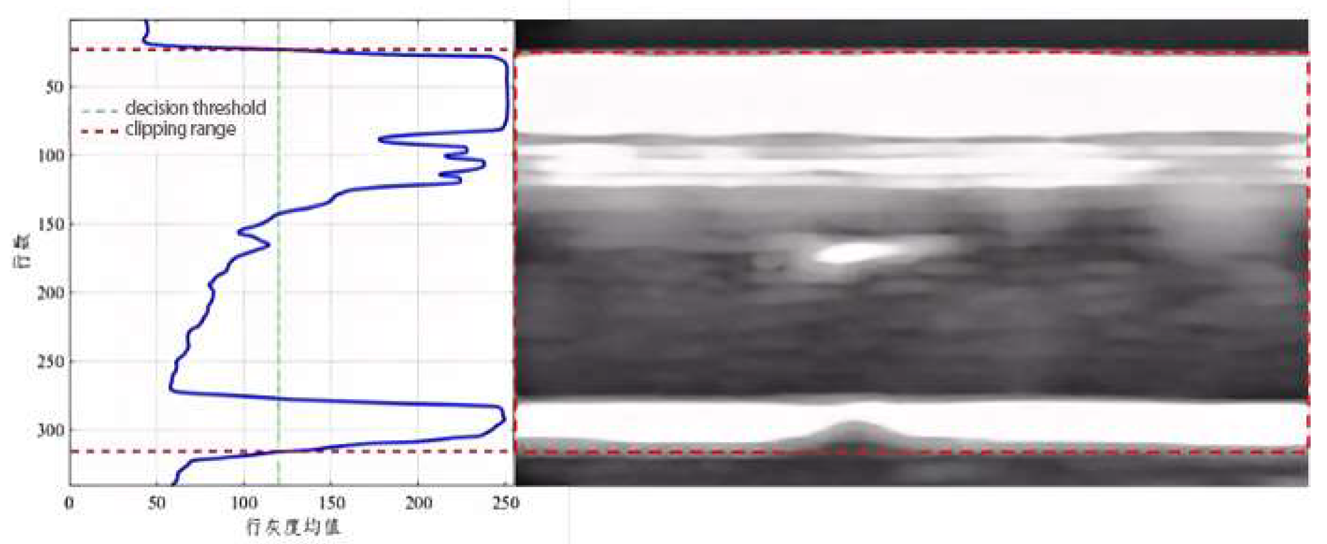
Figure 8.
binarized recurrence plots under different thresholds.(a)original image;(b)5% recurrence points proportion;(c)30% recurrence points proportion;(d)30% recurrence points proportion.
Figure 8.
binarized recurrence plots under different thresholds.(a)original image;(b)5% recurrence points proportion;(c)30% recurrence points proportion;(d)30% recurrence points proportion.
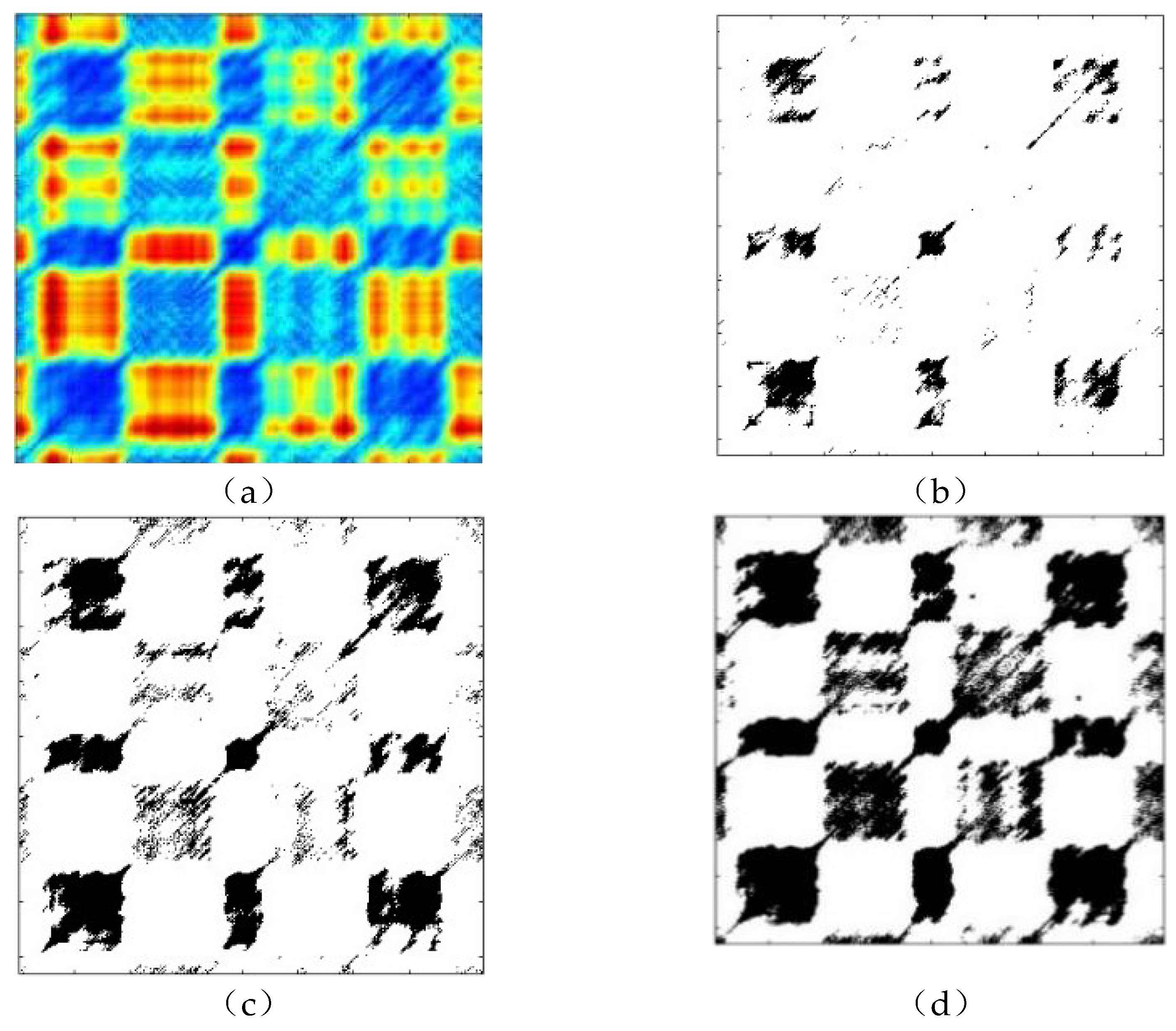
Figure 9.
Normalized Filter.
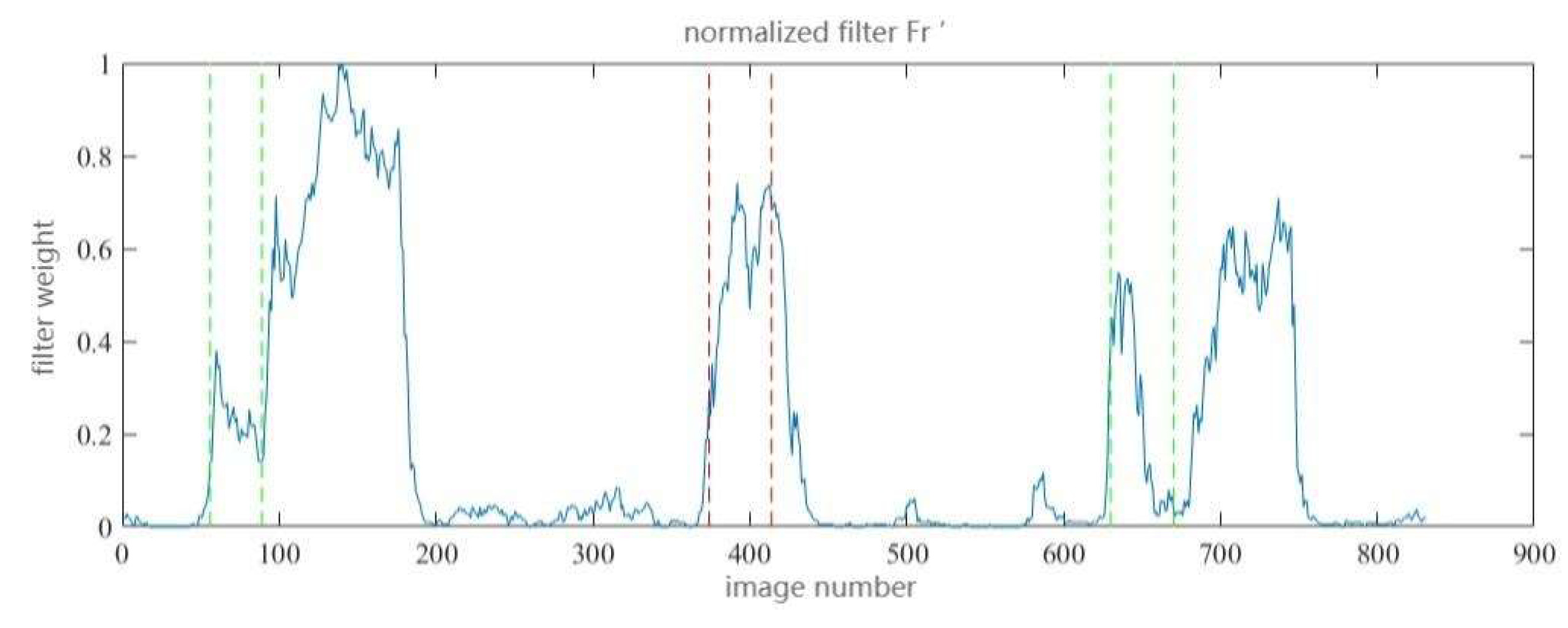
Figure 10.
Filtered Image Entropy Sequence.
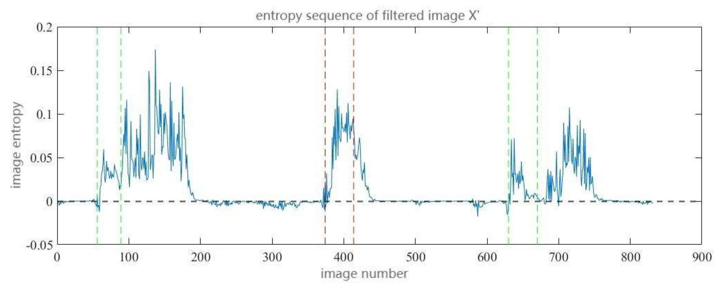
Figure 11.
Image Entropy Variation Sequence.
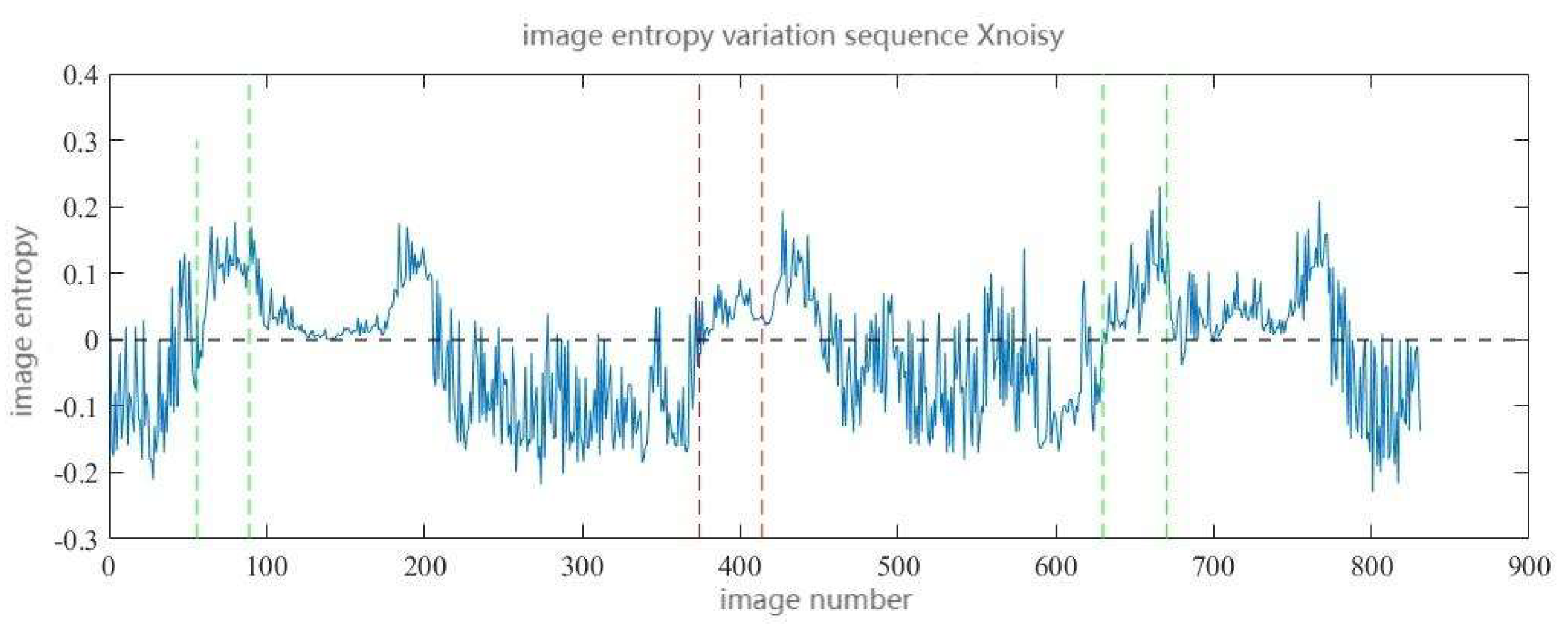
Figure 12.
Preprocessed Image of Experimental Sequence.
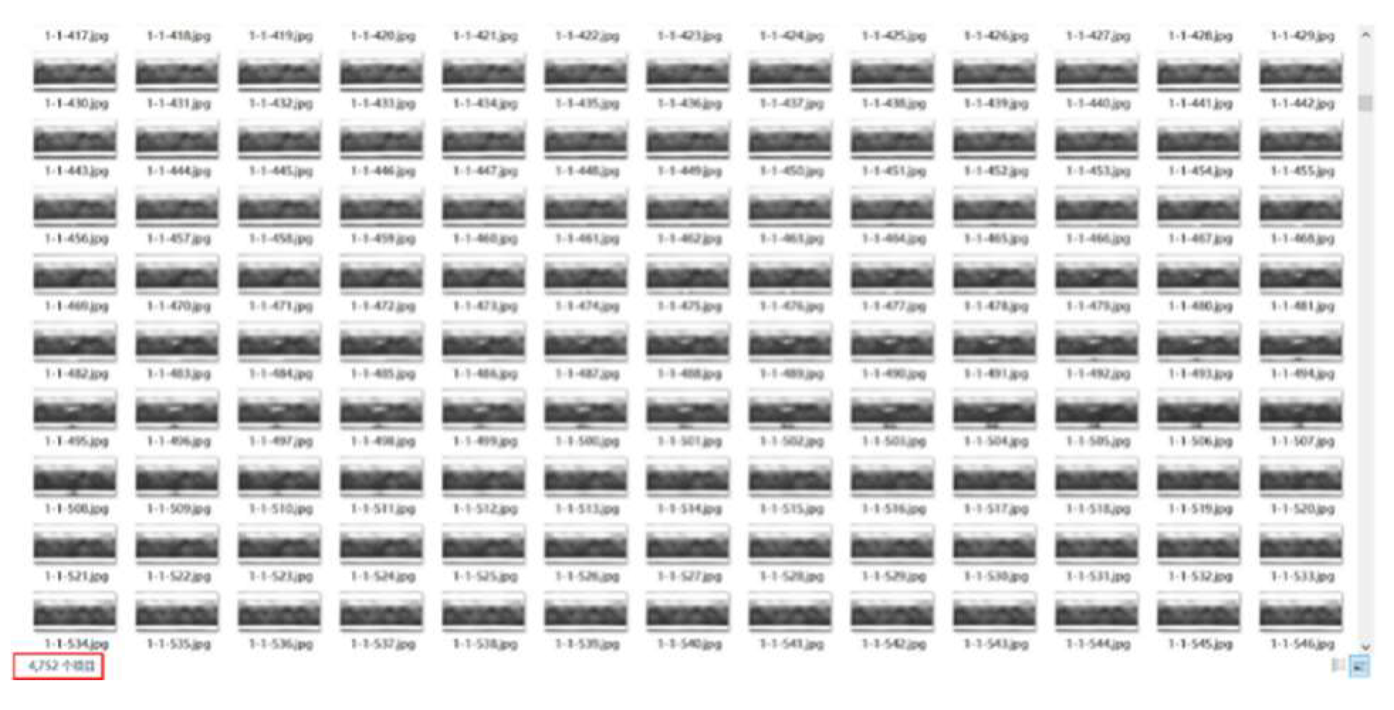
Figure 13.
Experimental Sequence.
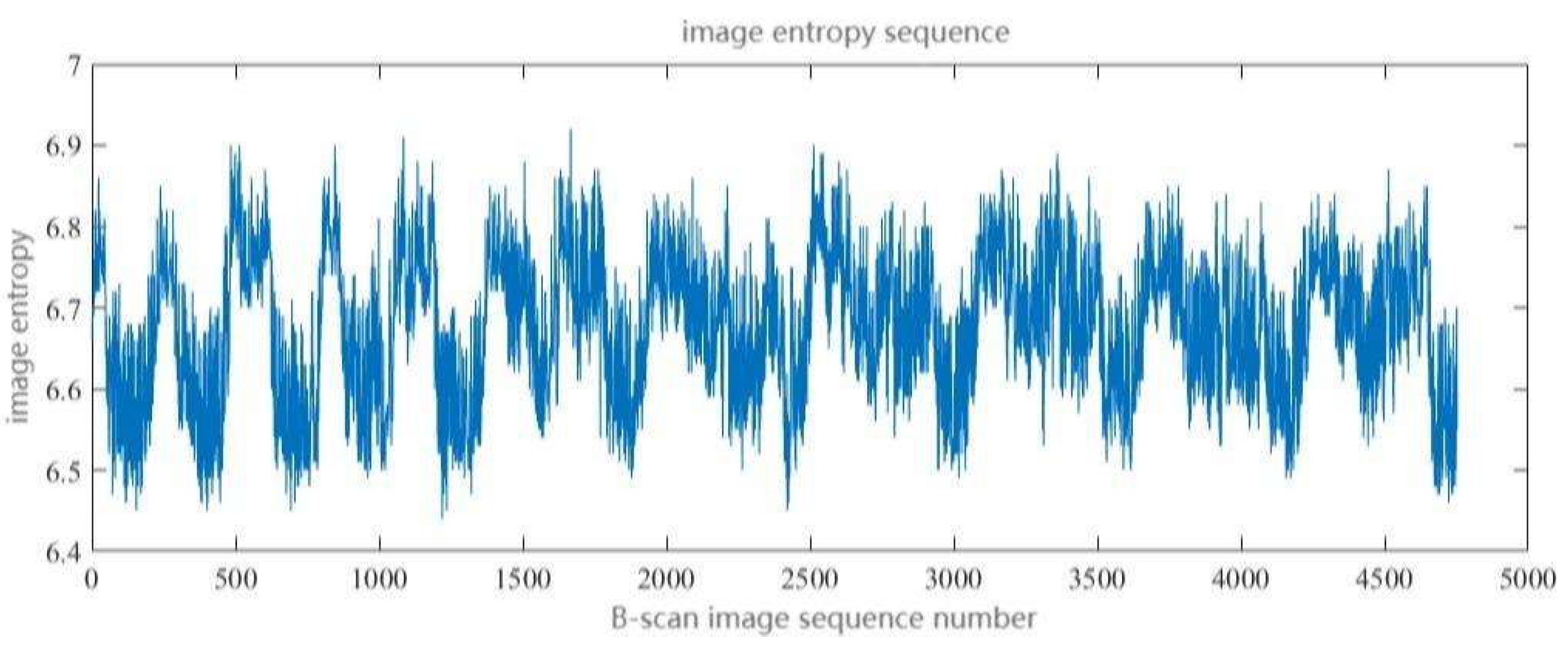
Figure 14.
Display of Recurrence Method Screening Results.(a) Threshold-free Recurrence Plot of Experimental Sequence;(b) Binarized Recurrence Plot of Experimental Sequence;(c) Normalized Filter of Experimental Sequence;(d) Filtered Image Entropy of Experimental Sequence;(e) Image Entropy Variation of Experimental Sequence;(f) Histogram of Recurrence Method Results of Experimental Sequence.

Disclaimer/Publisher’s Note: The statements, opinions and data contained in all publications are solely those of the individual author(s) and contributor(s) and not of MDPI and/or the editor(s). MDPI and/or the editor(s) disclaim responsibility for any injury to people or property resulting from any ideas, methods, instructions or products referred to in the content. |
© 2025 by the authors. Licensee MDPI, Basel, Switzerland. This article is an open access article distributed under the terms and conditions of the Creative Commons Attribution (CC BY) license (http://creativecommons.org/licenses/by/4.0/).
Copyright: This open access article is published under a Creative Commons CC BY 4.0 license, which permit the free download, distribution, and reuse, provided that the author and preprint are cited in any reuse.


