Submitted:
27 April 2025
Posted:
28 April 2025
You are already at the latest version
Abstract
This study addresses the critical challenge of insufficient classification accuracy for different defect signals in rail magnetic flux leakage (MFL) detection by proposing an intelligent classification method based on particle swarm optimized radial basis function neural network (PSO-RBF). The research systematically develops a comprehensive solution through three key aspects: experimental data acquisition, model architecture optimization, and performance validation. Initially, 400 sets of MFL signal samples were collected through artificial defect experiments, with six crucial MFL signal features selected as inputs for the 6-15-4 structured RBF network. To ad-dress the nonlinear mapping relationship between MFL signal characteristics and defect categories, an enhanced PSO algorithm incorporating dynamic learning factors and nonlinear inertia weight was implemented for RBF parameter optimization. Experimental results demonstrate significant performance improvements, with classification accuracy reaching 87.5% on artificial defect datasets (17.5 percentage points higher than conventional RBF), macro-F1 score increasing to 0.817, and MCC coefficient improving to 0.733. For actual defect detection with limited samples (100 sets), adaptive model adjustments including hidden layer reduction (10 neurons) and key feature weighting achieved 80% accuracy, while particularly improving minority class performance ("spalling" F1-score increased by 0.25 with 50% false alarm reduction). The proposed PSO-RBF model effectively enhances MFL signal feature extraction capability through precise optimization of center positions and kernel width parameters, demonstrating superior discriminative ability for various defects (abrasions, spalling, indentations, shelling) and providing an effective intelligent solution for rail defect classification in MFL detection.
Keywords:
rail defect detection
; magnetic flux leakage (MFL) testing
; feature selection
; intelligent classification
; model optimization
; imbalanced data
1. Introduction
As critical infrastructure for railway transportation, rails directly determine the safety and efficiency of railway systems. During long-term operation, the rail surface is prone to various types of defects—including abrasions, spalling, indentations, and shelling—due to rolling contact fatigue (RCF) with vehicle wheelsets [1]. These defects not only compromise the rail’s wear resistance and fatigue strength but also significantly affect its electromagnetic properties and other key performance indicators, thereby severely threatening rail service life and operational safety.
Conventional ultrasonic testing methods face inherent limitations in their detection principles, making it challenging to achieve efficient and accurate inspection of rail surface defects [2]. Consequently, substantial manual field inspections remain necessary in actual railway operations, failing to meet the demands of modern railway development.
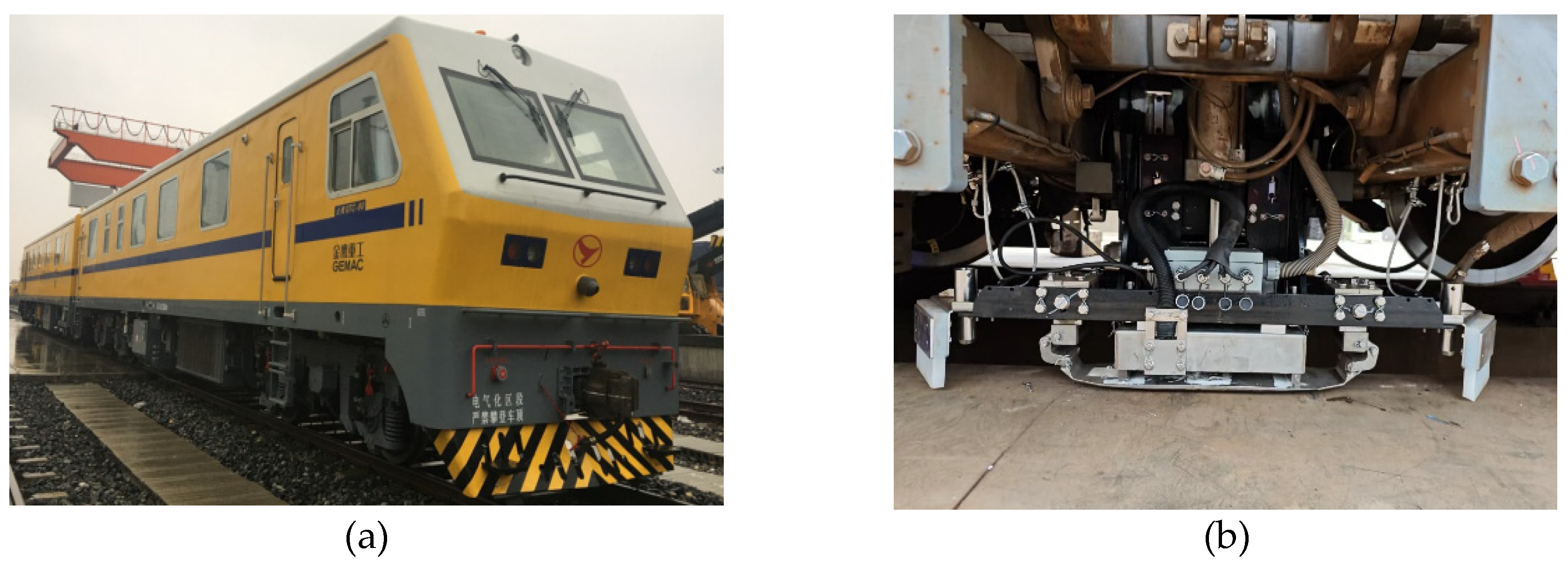
To address this issue, the China Academy of Railway Sciences, in collaboration with Professor Wang Ping’s team from Nanjing University of Aeronautics and Astronautics and Gemac Engineering Machinery Co., Ltd., jointly developed the GTC-80Ⅱ large-scale rail inspection vehicle. Equipped with an advanced electromagnetic detection system for rail head defects, this vehicle can effectively identify abrasions, spalling, indentations, shelling, and other defects on the rail running surface. Based on high-speed DC leakage flux testing technology, the system achieves inspection speeds up to 350 km/h under laboratory conditions. Compared with traditional ultrasonic techniques, it demonstrates superior advantages including higher speed, improved accuracy, elimination of couplant requirements, and the capability to detect near-surface defects (within 8 mm depth).
Nevertheless, despite the outstanding performance of this electromagnetic detection system in defect identification, significant challenges persist in the classification of electromagnetic signals. Currently, there lacks an effective methodology to accurately recognize and differentiate various types of defect signals. This study therefore aims to develop a deep learning-based classification model to enhance the accuracy of rail surface defect signal classification, thereby providing more reliable decision support for railway maintenance.
Figure 1.
Rail magnetic flux leakage detection system: (a) GTC-80 rail inspection vehicle. (b) rail magnetic flux leakage (MFL) detection probe.
Figure 1.
Rail magnetic flux leakage detection system: (a) GTC-80 rail inspection vehicle. (b) rail magnetic flux leakage (MFL) detection probe.
With the rapid development of modern railway systems, rail defect detection technologies face increasingly stringent challenges. Although existing methods have achieved notable improvements in stability and efficiency, traditional manual classification approaches exhibit evident limitations when processing massive volumes of suspected defect signals. Such experience-dependent subjective judgment not only suffers from inconsistent accuracy and low efficiency but also proves difficult to standardize due to its inherent nonlinearity and strong coupling characteristics [3]. Consequently, developing intelligent automated defect recognition and classification systems holds substantial engineering value for achieving precise rail defect prevention and scientific maintenance, ultimately ensuring railway operational safety.
In practical applications, defect signals collected by leakage flux inspection systems are often contaminated by multiple interference factors. Research indicates that three-dimensional mechanical vibrations during train operation cause signal baseline drift, while electromagnetic interference along tracks introduces high-frequency noise, collectively reducing the signal-to-noise ratio (SNR) of valid signals below 15dB [4]. Furthermore, rail surface defects typically exhibit the following characteristics: small geometric dimensions, irregular morphologies (e.g., discontinuous distribution patterns of shelling), and significant feature overlap between defect categories (e.g., < 10% amplitude difference in magnetic signals between abrasions and spalling). These factors persistently limit the accuracy of conventional threshold-based classification methods.
2. Related Works
From a pattern recognition perspective, rail defect classification fundamentally constitutes a nonlinear mapping problem from high-dimensional feature space to discrete category space [5]. Artificial neural networks (ANNs) demonstrate unique advantages in this domain due to their exceptional nonlinear system modeling capabilities. Among them, BP neural networks have become the preferred classifier architecture in engineering applications, owing to their excellent nonlinear approximation properties (theoretically capable of approximating any continuous function with arbitrary precision), modular hardware implementation characteristics, and generalization ability achieved through regularization techniques. Probabilistic neural networks (PNNs) employ Parzen window functions for probability density estimation, requiring only single-pass sample training with O(n) time complexity, making them particularly suitable for real-time online classification tasks [6].
However, existing neural network approaches still face unresolved technical challenges: BP networks are prone to local minima and exhibit sensitivity to hyperparameters like learning rates [7]; although PNNs train rapidly, their classification performance heavily depends on smoothing factor selection, with memory consumption growing linearly with training sample size. These limitations drive ongoing exploration of more advanced intelligent algorithms to address key technical bottlenecks in rail defect classification.
Recent years have witnessed significant advancements in rail defect classification research driven by machine learning and intelligent algorithms. As demonstrated in literature [8], a Fast R-CNN based approach was proposed for rail crack detection, where feature extraction and classification of rail defect images achieved high-precision damage identification, confirming the applicability of deep learning in rail flaw detection. Literature [9] employed Random Forest (RF) algorithm for multi-class prediction of fault data, with results indicating that this method maintains strong robustness even in noisy environments, though it exhibits notable dependence on feature engineering.
With the introduction of optimization algorithms, literature [10] utilized Genetic Algorithm (GA) to optimize the kernel function parameters of Support Vector Machine (SVM), thereby improving the accuracy of defect classification, albeit at the cost of increased computational complexity. Literature [11] proposed an RBF neural network model based on Adaptive Particle Swarm Optimization (APSO), which demonstrated fast convergence speed and high classification accuracy on rail defect datasets, providing novel insights into the application of intelligent optimization algorithms for damage prediction. These studies collectively highlight both the promising potential and existing challenges of intelligent algorithms in advancing rail defect detection technologies.
Nevertheless, existing methods still exhibit limitations: traditional BP networks easily converge to local optima with low training efficiency; SVMs incur substantial computational overhead for large datasets; while RBF neural networks possess strong nonlinear fitting capabilities, their center selection and width parameter optimization still rely on empirical adjustment [12]. To address these issues, this study proposes an improved MI-PSO-RBF model, incorporating multimodal information (MI) fusion to enhance feature representation and adaptive PSO-optimized RBF network parameters [13], thereby improving both accuracy and generalization performance in rail defect classification.
3. Rail Magnetic Flux Leakage Detection Technology
As a critical non-destructive testing (NDT) method, MFL technology is widely employed for defect detection in ferromagnetic materials [14]. The principle relies on magnetic field induction and material magnetization, where an external magnetic field is applied to the test specimen. Surface or near-surface defects (e.g., cracks, fatigue, or deformations) disrupt the magnetic flux distribution, generating detectable leakage fields. Through advanced signal processing, these anomalies are analyzed to determine defect characteristics (location, geometry, and dimensions). This technology significantly enhances industrial equipment safety by enabling early failure prevention, thereby reducing maintenance costs and production downtime.
Rail Defect Detection Mechanism
During rail inspection, localized magnetization ensures magnetic flux lines intersect potential defects. When surface/subsurface defects exist, the permeability contrast between steel and air causes flux leakage at defect sites according to the principle of magnetic flux continuity. The key challenge lies in interpreting these leakage signals for defects with complex morphologies.
Figure 2.
Schematic Diagram of Magnetic Flux Leakage (MFL) Detection Principle.
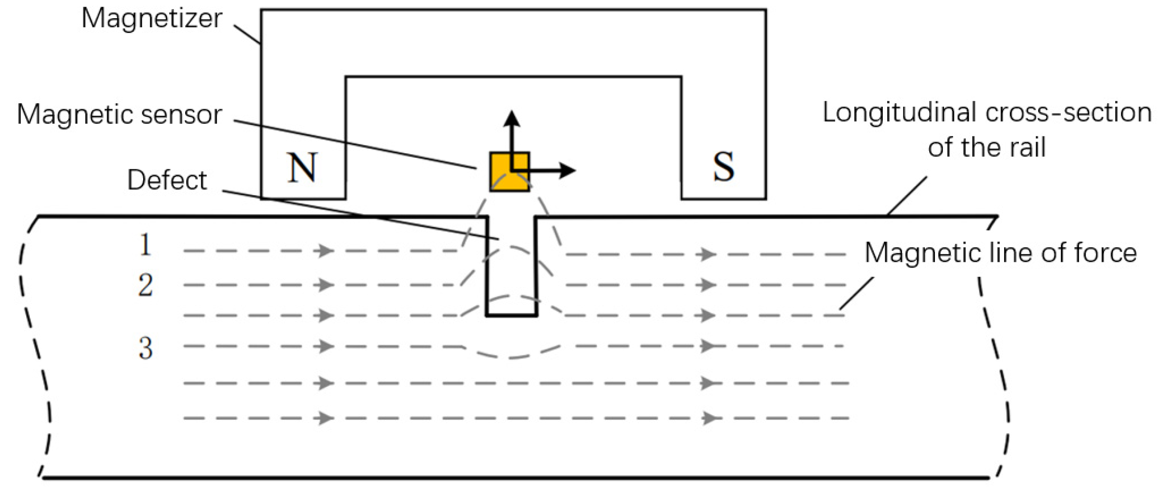
In actual railway lines, rail defects often exhibit irregular shapes with significant dimensional variations, undoubtedly increasing the difficulty of defect classification and quantitative analysis. Nevertheless, different types of defects still demonstrate certain correlations in their effects on magnetic flux leakage (MFL) signals. For instance, defect depth primarily influences signal amplitude, while defect width affects peak spacing and peak area in MFL signals. Meanwhile, defect irregularity is reflected in signal skewness, kurtosis, and other higher-order statistical features. When multiple influencing factors collectively affect defect signals, the resulting complexity makes it impossible to accurately characterize them using simple formulas or analytical functions. To address this challenge, this study adopts a radial basis function (RBF) neural network approach to decouple and analyze defect signals, systematically investigating the relationship between signal characteristics and different defect types to achieve effective classification of MFL signals.
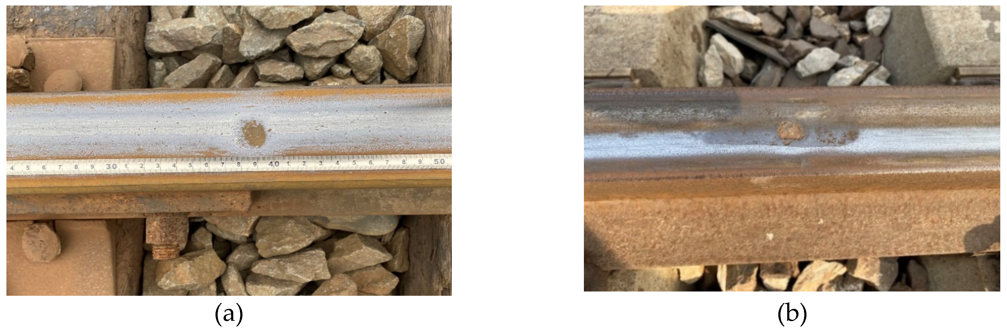
During railway operation, rails serve as critical infrastructure components that endure long-term wheel-rail contact stresses, frictional forces, and various external factors, inevitably leading to the formation of diverse natural defects. These defects not only significantly reduce rail service life but may also pose serious threats to operational safety. Common rail surface defects include rail abrasions, spalling, surface indentations, and gauge corner shelling [15].
Rail Defect Types and Signal Characteristics:
In operational railways, four predominant defect types are observed:
1.Rail abrasion (Depth: 0.5-2 mm; Length: 20-100 mm): Caused by wheel slippage during acceleration/braking, typically showing 4-20 abrasion marks per rail.
2.Rail spalling (Width: 3-8 mm; Max depth: 3 mm): Occurs at curve outer edges, characterized by discontinuous material loss due to rolling contact fatigue.
3.Rail indentation: Results from foreign object intrusion, forming isolated or periodic pits on the railhead.
4.Shelling: Fatigue-initiated microcracks that propagate into fish-scale patterns, primarily in high-stress zones.
Figure 3.
Four typical types of natural rail defects: (a) Rail abrasion. (b) Rail spalling. (c) Rail indentation. (d) Shelling.
Figure 3.
Four typical types of natural rail defects: (a) Rail abrasion. (b) Rail spalling. (c) Rail indentation. (d) Shelling.
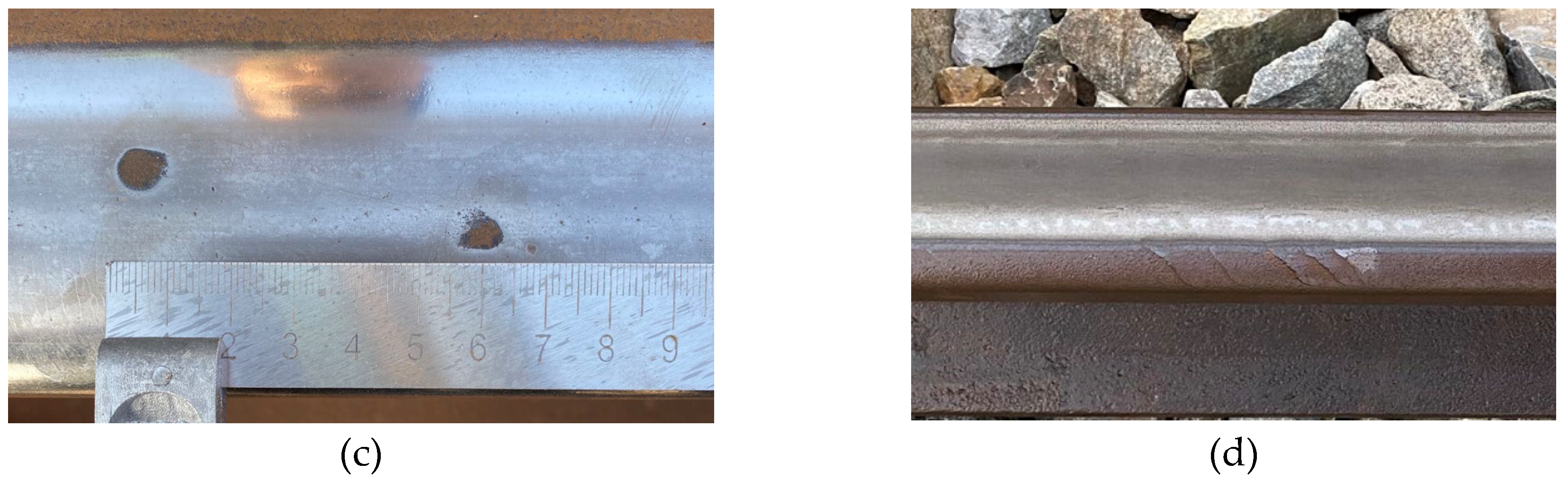
Given the considerable challenges associated with obtaining diversified defect samples from actual railway tracks, this study proposes a field-verified defect sample collection methodology. Specifically, through comprehensive analysis of acquired suspected defect signals combined with mileage information and marker locations, precise field positioning is achieved for on-site defect verification. While this process enables the acquisition of authentic defect data to a certain extent, the variety and quantity of samples remain constrained by field conditions, proving inadequate to meet the substantial demand for diverse samples required for model training and testing.
To overcome this limitation and ensure the reliability of the RBF neural network model in defect classification tasks, this study meticulously designed and fabricated a series of artificial defect rail samples. Through extensive experimentation, systematic acquisition of sample data under varying defect types and severity levels was accomplished, establishing a robust data foundation for model training and validation. These artificial defect samples encompass multiple prevalent defect types including cracks, abrasions, spalling, and indentations, with careful dimensional parameter planning and adjustment to comprehensively simulate the complex diversity of defects encountered in operational track conditions. Physical demonstrations of the artificial defect samples are presented as follows.
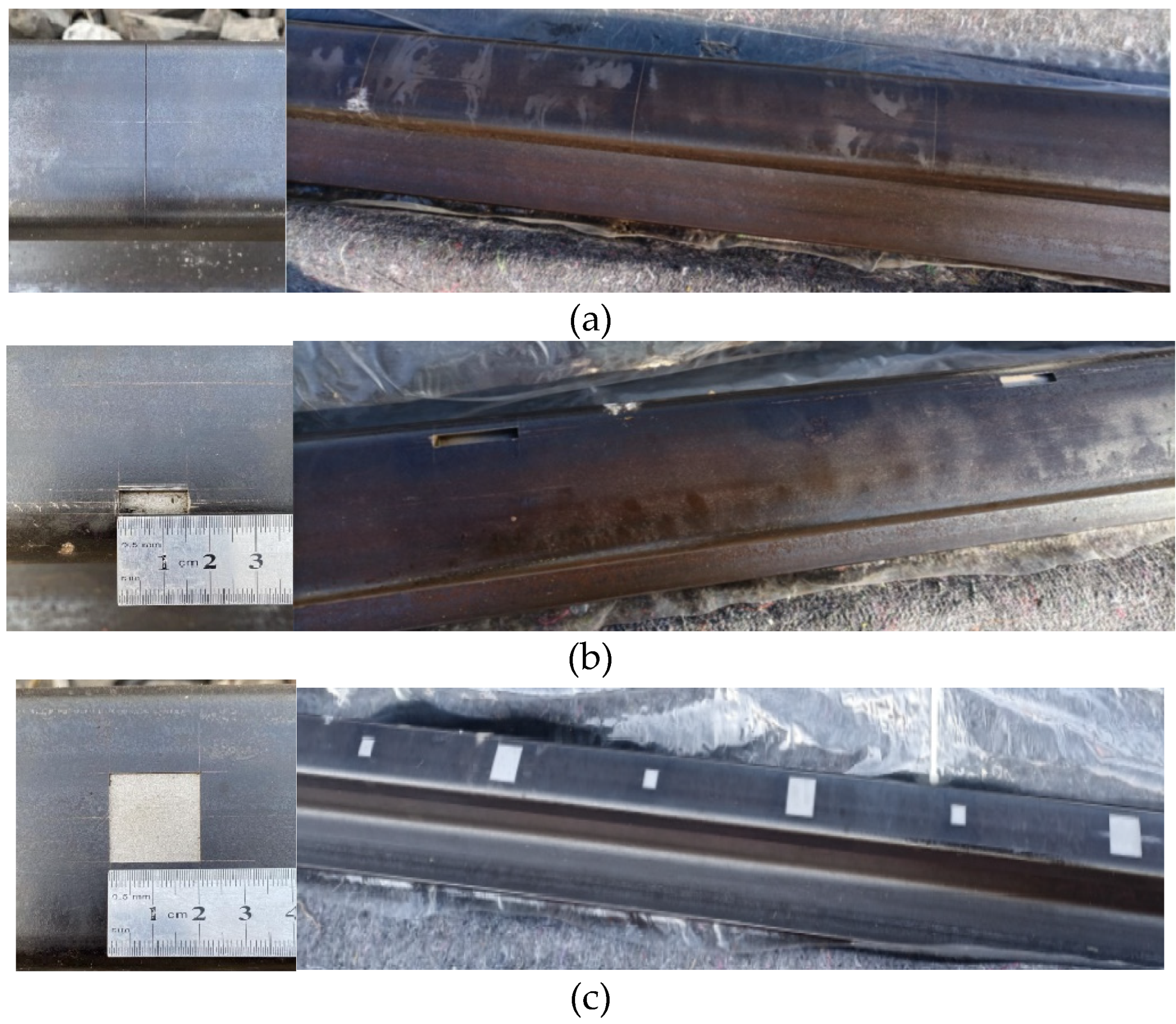
Figure 4.
Physical images of four types of artificial defects: (a) Physical image of artificial transverse crack defect on rail surface. (b) Physical image of artificial spalling defect at gauge corner. (c) Physical images of artificial defects: abrasion and indentation on rail surface.
Figure 4.
Physical images of four types of artificial defects: (a) Physical image of artificial transverse crack defect on rail surface. (b) Physical image of artificial spalling defect at gauge corner. (c) Physical images of artificial defects: abrasion and indentation on rail surface.
4. Methodology
4.1. Analysis of Magnetic Flux Leakage (MFL) Defect Signal Characteristics
Magnetic flux leakage (MFL) detection technology is widely used in defect detection due to its reliability and well-established principles. By analyzing changes in MFL signals, different types of defects can be effectively identified. Through quantitative analysis of signal characteristics, distinct patterns of various defects can be revealed, which is essential for building an accurate classification system.
Based on existing research and our study on rail surface defects [16], we selected nine key features that effectively distinguish different defect signals:
1.Peak-to-peak value: The difference between the maximum and minimum values of a signal, used to measure the amplitude range.
2. Peak-to-peak interval: The interval between two adjacent peaks, commonly used to analyze periodic characteristics of signals.
3.Peak area: The area under a signal peak, which can be calculated by integrating the peak region.
4.Peak-to-peak slope: The slope variation during the transition from one peak’s decline to another peak’s rise, reflecting the signal’s rate of change.
5.Mean value: The arithmetic average of all sample values, representing the central tendency of the signal.
6.Crest factor: The ratio of the signal’s peak value to its RMS value, indicating the relationship between peak amplitude and average power.
7.Kurtosis: A measure of the “tailedness” of a real-valued random variable’s probability distribution, describing the sharpness and heaviness of the signal’s tails.
8.Root Mean Square (RMS): The effective value of a signal, representing its power-equivalent magnitude.
9.Skewness: A measure of the asymmetry of a real-valued random variable’s probability distribution, describing the signal’s distributional bias.
4.2. RBF Neural Network Architecture
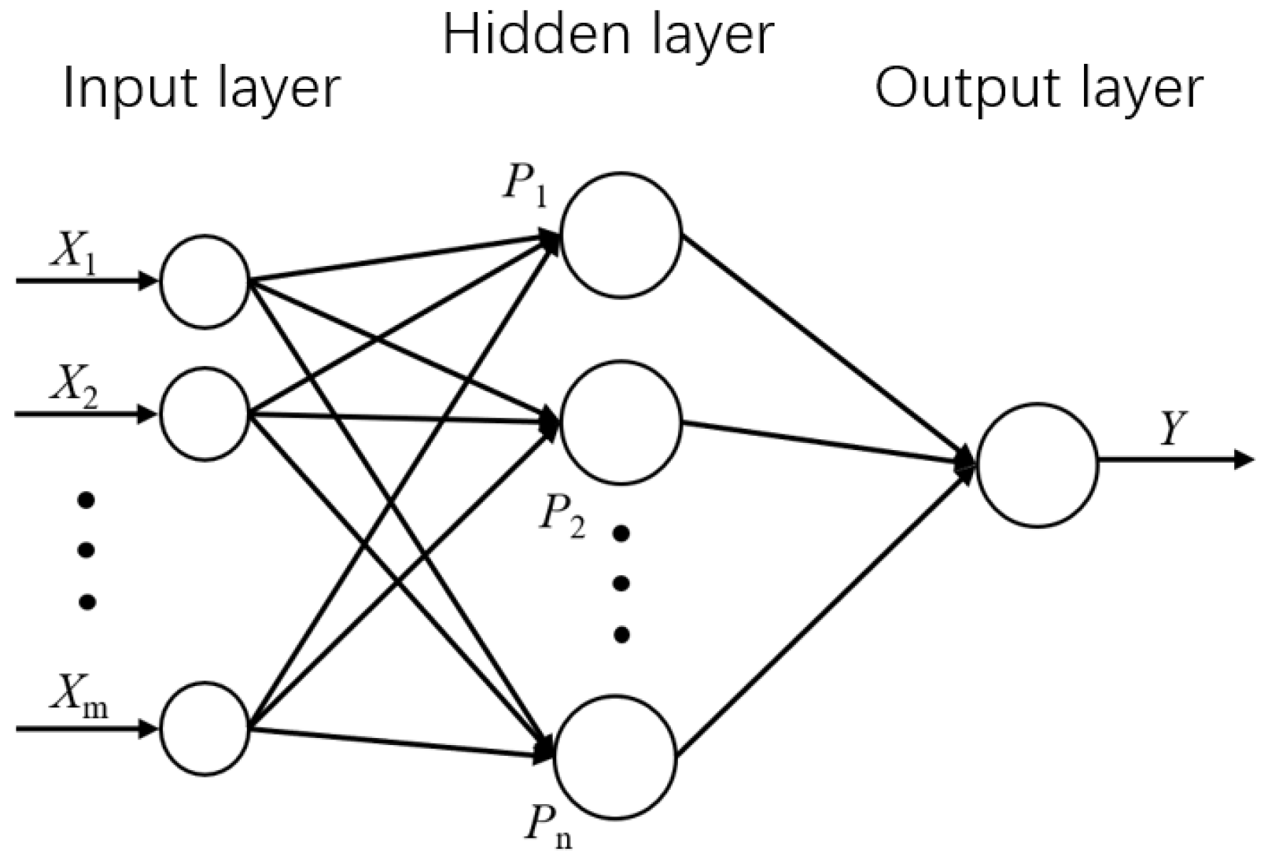
The Radial Basis Function (RBF) neural network represents an efficient feedforward neural network architecture, whose core principle lies in utilizing radial basis functions as the “basis” for hidden layer units. This unique structure enables nonlinear mapping between the input and hidden layers while maintaining linear mapping between the hidden and output layers. Such distinctive network configuration endows RBF networks with significant advantages in handling nonlinear problems, demonstrating superior convergence speed and nonlinear approximation capabilities compared to the widely-used BP neural networks.
The RBF network comprises three fundamental components: the input layer, hidden layer, and output layer. The input layer serves to receive external input signals and transmit them into the network. Assuming the input layer contains m nodes, each node corresponds to one dimension of the input signal. The hidden layer, as the critical component of the RBF network, performs nonlinear transformation of input signals. The number of neurons in the hidden layer typically relates to the complexity of training data. Assuming the hidden layer contains n nodes, each node corresponds to a radial basis function. These basis functions, centered on the input signals, generate nonlinear features by computing the distance between input signals and center points. The hidden layer connects to the output layer through weight vector w, and the output layer produces the final network output through linear combination of hidden layer outputs.
Figure 5.
Topological structure of RBF neural network.
In practical applications, the Gaussian basis function—positive definite in arbitrary space—is commonly selected as the hidden layer function for RBF neural networks, as expressed in Equation (1):
Where:
pj represents the vector of the j-th neuron in the hidden layer;
x denotes the neural network input sample;
cj indicates the center vector of the j-th hidden layer node, with dimensionality identical to the input sample;
δj corresponds to the width of the j-th hidden layer node.
The linear relationship in the output layer of the RBF network is expressed by Equation (2):
Where:
y represents the computed output value of the neural network;
wj signifies the weight vector between the j-th hidden layer neuron and the output layer;
n denotes the number of hidden layer neuron nodes.
Although RBF neural networks demonstrate excellent capability in handling nonlinear problems, the determination of network parameters critically influences model outputs. Therefore, the identification of several key parameters—including the RBF center cj, normalization constant, and weight coefficients wij between the hidden and output layers—becomes particularly crucial.
4.3. Feature Selection Using Mutual Information
In magnetic flux leakage (MFL) detection technology, the extracted signal features typically exhibit multi-dimensional characteristics. For instance, nine distinct feature values derived from MFL signals constitute continuous feature sets for each sample, including but not limited to peak-to-peak amplitude, peak spacing, peak area, and other relevant parameters. However, directly employing all these continuous features as inputs for artificial neural networks not only consumes substantial computational resources but may also compromise prediction accuracy due to interference from irrelevant features.
To address this challenge, we employ the Mutual Information (MI) criterion for feature selection and dimensionality reduction [17]. Mutual information serves as a robust metric for quantifying the mutual dependence between two variables, particularly suitable for evaluating the correlation between continuous features and discrete defect categories. The calculation formula for mutual information is expressed as follows:
Where:
• p (x, y) represents the joint probability of feature X taking value x and defect category Y taking value y
• p (x) denotes the marginal probability of feature X taking value x
• p (y) indicates the marginal probability of defect category Y taking value y
In practical applications, these probabilities can be estimated by analyzing the frequency distribution within the dataset. For continuous features, probability density functions are typically estimated using kernel density estimation methods, from which both marginal and joint probabilities can be derived.
By computing mutual information values between defect signal features and defect categories, we can identify the most relevant features for defect classification, which are subsequently utilized for predictive model training and validation. This approach significantly enhances prediction accuracy while reducing computational overhead.
The mutual information calculation can alternatively be implemented through a parameter-free k-nearest neighbor (KNN) based method. This technique employs the maximum Euclidean distance in both X and Y directions as the criterion for nearest neighbor selection, followed by statistical counting and probability density estimation. This methodology not only effectively handles the complex relationships between continuous features and discrete labels but also preserves the most critical information during feature selection, thereby improving both model performance and computational efficiency.
Through these methods, we can efficiently extract the most valuable features from high-dimensional data, establishing a robust foundation for subsequent neural network training and defect classification tasks.
4.4. PSO Algorithm for Parameter Optimization
The particle swarm optimization (PSO) algorithm simulates the foraging behavior of bird flocks [18], where each particle’s position represents a potential solution. During iterations, particles move toward their individual historical best positions. In an M-dimensional search space, xi = (xi1, xi2, …, xiM), vi = (vi1, vi2, …, viM)), and pi = (pi1, pi2, …, piM) respectively denote the position, velocity, and personal best position of the i-th particle, while g = (g1, g2, …, gM) represents the global best position of the swarm. The velocity and position update equations are given by Equation (4) and (5):
Where:
vid ∈ [-vmax, vmax], vmax = k·xmax (d: dimension index; i: population size)
t: iteration count
w: inertia weight
c1 and c2: learning factors
r1 and r2: random numbers uniformly distributed in (0,1)
Vid: maximum velocity
The parameters w, c1 and c2 critically influence the algorithm’s global search capability and convergence speed. Reference demonstrates that larger w values facilitate broader exploration during initial stages, while smaller values enable precise local search later. Reference proposes linear variation of w, but premature reduction may trap particles in local optima. To address this, we design a piecewise nonlinear decreasing strategy (Eq.6). Excessive c1 values restrict particles to local regions, while insufficient c2 values cause premature convergence. Accordingly, we implement linear decrease for c1 and linear increase for c2 (Eq.7).
Where:
In the formula: wmax is the upper limit of the inertia weight, wmin is the lower limit of the inertia weight, generally taken as wmax = 0.9, wmin = 0.4, ger represents the maximum number of iterations, and t denotes the current iteration count.
In the formula: ci_max represents the maximum value of the i-th learning factor; ci_min represents the minimum value of the i-th learning factor.
This approach ensures: 1) rapid global exploration initially through higher velocities, 2) balanced transition via nonlinear deceleration, and 3) enhanced local refinement while avoiding linear decrease’s limitations. Equation (8) shows larger c1 and smaller c2 during early stages promote global coverage, while reversed settings in later stages improve local optimization.
The PSO-RBF optimization maps neural network parameters to particle positions, using minimum mean square error as the fitness function to determine optimal weights. The complete algorithm flowchart is presented in Figure 6.
5. Experimental Validation
5.1. Experimental Setup
The magnetic flux leakage (MFL) detection system is mounted on a GTC-80 rail inspection vehicle for high-speed rail inspection [19]. The system consists of core components including an industrial computer, signal conditioning circuit, data acquisition card, power supply box, and detection probes. The detection probes employ an array of Hall sensors (single sensor size: 1.5 × 1.5 mm², minimum center spacing: 2 mm) installed between the wheel sets of the bogie. During inspection, the train moves at a constant speed of 40 km/h, while the magnetizers and sliding shoes positioned before and after the probes work in coordination to achieve continuous scanning of rail defects. The signals are biased and amplified by an AD620 instrumentation amplifier and then stored in real time by the data acquisition system. After detection, dedicated playback software is used to locate suspected defect signals, which are then manually verified to confirm the damage location [20].
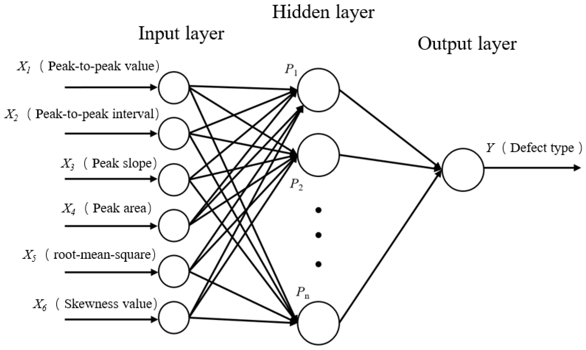
This study evaluates the relevance of different features to defect categories through Mutual Information (MI) analysis. The results indicate that six features—root mean square (0.5926), skewness (0.7323), peak area (0.6201), peak slope (0.6629), peak spacing (0.7232), and peak-to-peak value (0.6636)—exhibit significantly higher MI values compared to other features (e.g., mean value: 0.2813, crest factor: 0.4132, kurtosis: 0.3532). This suggests that these six features possess stronger discriminative power for defect classification. Based on this finding, the study selects them as input variables for the classification model.
In model construction, the dataset is divided into an 80% training set and a 20% test set. A six-input single-output prediction model is established, with peak-to-peak value, peak spacing, peak slope, peak area, root mean square, and skewness as input units and defect type as the output. The hidden layer parameters are optimized using a Particle Swarm Optimization (PSO) algorithm, ultimately forming a rail defect prediction model.
Figure 8.
Topological structure of RBF prediction model.
5.2. Evaluation Index System
To comprehensively assess model performance, this study employs the following four evaluation metrics:
1.Accuracy (Acc)
Where:
TP: Number of true positive predictions
TN: Number of true negative predictions
FP: Number of false positive predictions
FN: Number of false negative predictions
This metric reflects overall classification correctness but exhibits sensitivity to class imbalance.
2.Macro-F1 Score
Where C represents the number of classes (C = 4 in this study).
This measure balances precision and recall for each defect category, providing equal weight to all classes regardless of their sample sizes.
3.Matthews Correlation Coefficient (MCC)
Particularly suitable for imbalanced datasets, MCC ranges from [-1,1], where 1 indicates perfect prediction performance.
4.Kappa Coefficient
This statistic evaluates the agreement between classification results and random chance, with values > 0.8 indicating excellent agreement beyond random classification.
5.3. Artificial Defect Experimentation and Results Analysis
The experimental study employed 400 annotated samples (160 abrasions, 120 spallings, 80 indentations, and 40 cracks) in artificial defect experiments, with an 8:2 ratio for training and testing sets. A three-layer RBF neural network architecture (6-15-4) was implemented, where the input layer processed six standardized features including peak-to-peak value and peak spacing, the hidden layer contained 15 Gaussian neurons with centers initialized via K-means++ algorithm to enhance convergence efficiency, and the output layer utilized Softmax activation for probabilistic classification of four defect types. For network optimization, the Particle Swarm Optimization (PSO) algorithm was configured with 20 particles (each as a 120-dimensional vector encompassing centers, widths of 15 neurons, and output weights), dynamic learning factors (c₁ linearly decreasing from 1.8 to 0.5, c₂ linearly increasing from 0.5 to 1.8), nonlinear inertia weight decay (initial value 0.9, decay coefficient β = 0.95), and a maximum of 200 iterations with early stopping condition (fitness change < 1×10⁻⁴ for 20 consecutive generations).
Comparative analysis: Confusion matrices of conventional RBF predictions, PSO-RBF predictions, and their key performance metrics.
Figure 9.
Confusion matrix of artificial defect prediction results using conventional RBF.
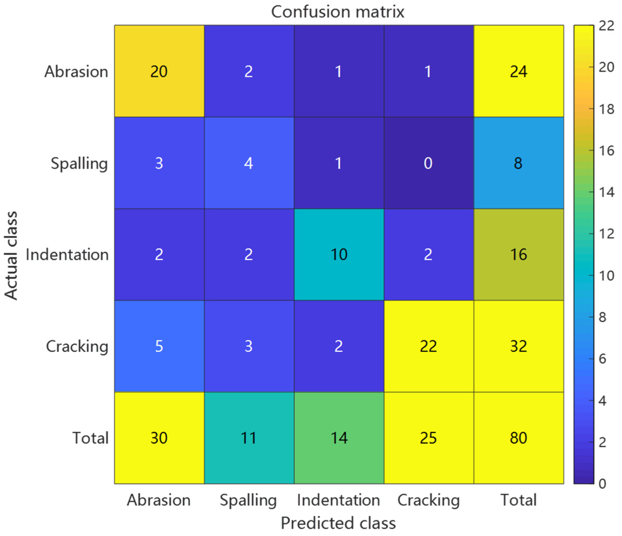
Figure 10.
Confusion matrix of artificial defect prediction results using PSO-RBF.
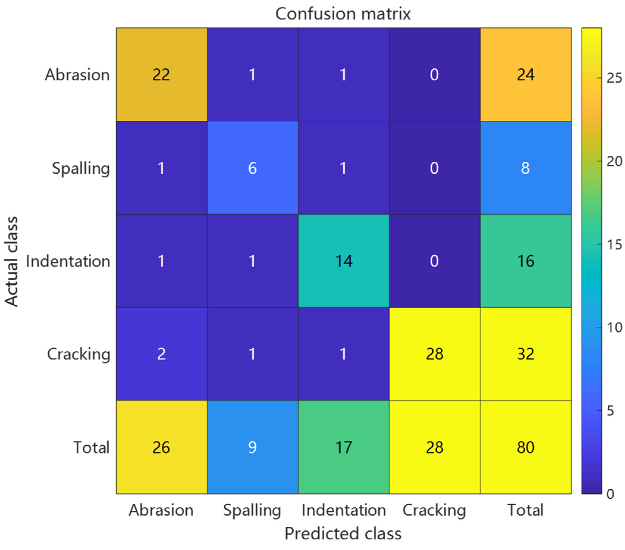

Table 1.
Comparison of key performance metrics for artificial defect prediction results.
| Metric | Accuracy | Macro-Average F1 Score | MCC | Kappa Coefficient |
|---|---|---|---|---|
| Conventional RBF | 0.7 | 0.645 | 0.548 | 0.573 |
| PSO-RBF | 0.875 | 0.817 | 0.733 | 0.818 |
| Improvement Margin | +0.175 (25%) | +0.172 (27%) | +0.338(34%) | +0.245 (43%) |
Comparative analysis revealed that the PSO-optimized RBF model achieved significant performance improvements over the conventional RBF approach. The overall accuracy increased from 70.0% to 87.5%, while the Macro-F1 score improved from 0.645 to 0.817, demonstrating enhanced balance between precision and recall across all defect categories. The Matthews Correlation Coefficient rose from 0.548 to 0.733, and the Kappa coefficient improved from 0.573 to 0.818, confirming better classification consistency and robustness in handling class imbalance. Detailed class-specific analysis showed particularly notable improvements for minority classes: the spalling class exhibited a reduction in false positive rate from 43.8% to 18.8% with F1 score increasing by 0.2667, while the crack class saw missed detections decrease from 10 to 4 cases with F1 score improving by 0.1614. These enhancements stemmed from PSO’s precise adjustment of RBF centers (e.g., 38.6% reduction in Euclidean distance for spalling features) and adaptive optimization of kernel widths (e.g., 31.2% contraction in radial basis response range for cracks), while maintaining scratch recognition accuracy (F1 score slightly increased from 0.7407 to 0.8462). The synchronous improvement in both MCC and Macro-F1 scores further validated the model’s enhanced capability in addressing class imbalance challenges.
5.4. Actual Defect Experimentation and Results Analysis
Given the scarcity of actual defect data (100 samples comprising 30 abrasions, 20 spallings, 25 indentations, and 25 shellings), the model architecture underwent adaptive modifications to address this limitation. The hidden layer neurons were reduced to 10 to mitigate overfitting risks, while the PSO population size was correspondingly adjusted to 15 particles to balance computational efficiency with search capability. During feature processing, prior knowledge was incorporated to enhance the weights of peak spacing and skewness features (multiplied by coefficients of 1.5 and 1.3, respectively) to accommodate signal variations caused by the irregular morphology of actual defects. The optimization process maintained the 200-generation iteration limit but introduced a class weight compensation mechanism (50% increased weight for shelling defects) to alleviate the impact of imbalanced sample distribution on classification boundaries. All experiments were conducted under identical hardware conditions to ensure the comparability of time-consumption metrics.
Comparative analysis: Confusion matrices of conventional RBF predictions, PSO-RBF predictions, and their key performance metrics.
Figure 11.
Confusion matrix of actual defect prediction results using conventional RBF.
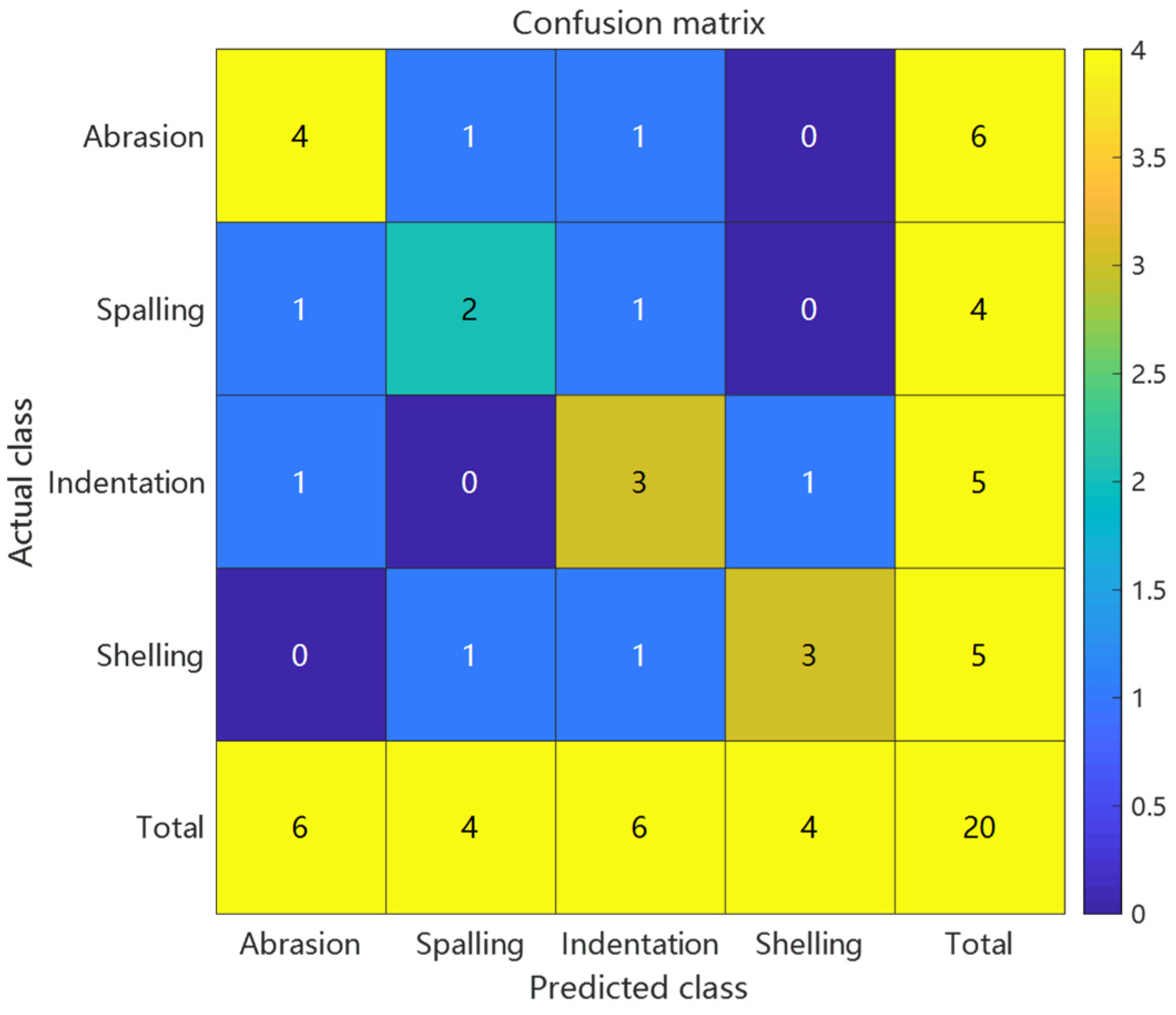
Figure 12.
Confusion matrix of actual defect prediction results using PSO-RBF.
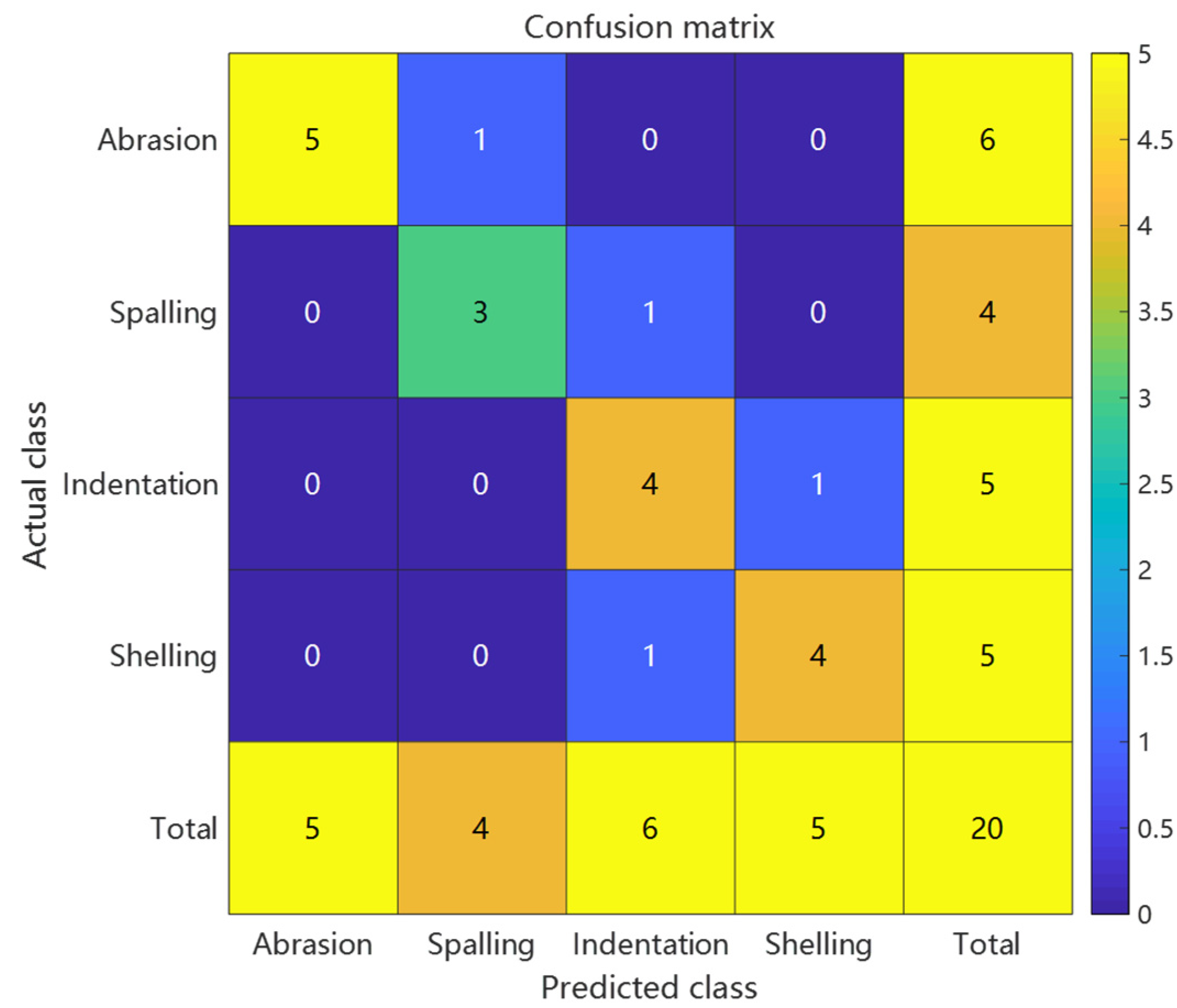
Table 2.
Comparison of key performance metrics for actual defect prediction results.
| Metric | Accuracy | Macro-Average F1 Score | MCC | Kappa Coefficient |
|---|---|---|---|---|
| Conventional RBF | 0.6 | 0.595 | 0.465 | 0.463 |
| PSO-RBF | 0.8 | 0.797 | 0.735 | 0.732 |
| Improvement Margin | +0.175 (25%) | +0.202 (34%) | +0.27 (58%) | +0.269 (58%) |
The PSO-RBF network model, obtained through particle swarm optimization of RBF network weight parameters, demonstrated significant improvements in defect classification performance. Comparative analysis between conventional RBF and PSO-RBF models revealed substantial enhancements across all key metrics: accuracy increased from 60% to 80%, Macro-F1 score improved from 0.595 to 0.797, Matthews Correlation Coefficient (MCC) rose from 0.465 to 0.735, and Kappa coefficient increased from 0.463 to 0.732. These improvements confirm that PSO optimization effectively enhanced both the overall classification accuracy and robustness of the model, particularly in addressing class imbalance challenges.
The most notable improvement was observed in the minority “spalling” class (F1 score increase of approximately 0.25), with false positive rate reduced from 50% to 25%. The optimized RBF kernel parameters also reduced false negatives by 1 case each for “indentation” and “crack” defects, while the 0.202 improvement in Macro-F1 score indicates more balanced recognition across different defect categories. The 0.09 increase in MCC confirms that PSO effectively reduced random guessing components, particularly enhancing the distinguishability of the least-represented “spalling” class (only 4 samples). These improvements primarily stem from PSO’s precise adjustment of RBF center positions and adaptive optimization of kernel widths, which maintained the recognition accuracy of majority classes while significantly improving classification performance for minority classes.
These results demonstrate that PSO optimization can effectively enhance the performance of RBF models in defect classification tasks, particularly in handling class imbalance problems with greater robustness. By optimizing RBF kernel parameters, the PSO-RBF model achieved significant improvements in both false positive and false negative reduction, thereby enhancing the overall classification accuracy and reliability of the model. The confusion matrix for the defect test set classification results using the PSO-RBF network model is shown in the accompanying figure, while the comparative table of key metrics between conventional RBF and PSO-RBF neural networks is presented in the following section.
6. Conclusion
This study presents an intelligent classification approach integrating Mutual Information (MI) feature selection and Particle Swarm Optimized Radial Basis Function (PSO-RBF) neural network to address the critical challenge of insufficient classification accuracy in rail defect detection using magnetic flux leakage (MFL) technology. The proposed methodology systematically employs MI criterion for feature screening and dimensionality reduction to identify the most discriminative feature subset strongly correlated with defect categories. The developed PSO-RBF model incorporates dynamic learning factors and nonlinear inertia weight strategies, demonstrating superior performance with 87.5% classification accuracy on artificial defect datasets (17.5 percentage points improvement over conventional methods) and maintaining robust adaptability (80% accuracy, 0.25 F1-score enhancement for minority classes) in actual defect detection scenarios. However, several limitations warrant further investigation: (1) constrained generalization capability due to limited actual defect samples; (2) sensitivity of MI feature selection to probability density estimation accuracy for continuous features; and (3) potential local optima trapping in PSO parameter optimization. Future research directions include: (1) employing Generative Adversarial Networks (GANs) for actual defect sample augmentation; (2) developing enhanced MI computation methods based on kernel density estimation; and (3) implementing hybrid optimization algorithms (e.g., PSO-GA) to further improve parameter optimization efficacy, ultimately advancing intelligent classification solutions for rail MFL inspection.
Author Contributions
Conceptualization, K.-L.J. and Y.-L.J.; methodology, P.W. and Y.-L.J.; software, K.-L.J.; validation, K.-L.J. and P.W.; formal analysis, K.-L.J.; investigation, K.-L.J.; resources, P.W.; data curation, K.-L.J.; writing—original draft preparation, K.-L.J.; writing—review and editing, P.W. and Y.-L.J.; visualization, K.-L.J.; supervision, P.W. and Y.-L.J.; project administration, Y.-L.J.; funding acquisition, P.W. All authors have read and agreed to the published version of the manuscript.
Funding
This work was funded by the Scientific Research Projects of China Academy of Railway Sciences under grant number 2023YJ330 and Jiangsu Province Scientific Research and Practical Innovation Program (KYCX21_0200).
References
- Antipov, A.G.; Markov, A.A. Detectability of rail defect by magnetic flux leakage method. Russian Journal of Nondestructive Testing, 2019, 55, 277–285. [Google Scholar] [CrossRef]
- He, Z.; Wang, Y.; Yin, F.; Liu, J. Surface defect detection for high-speed rails using an inverse P-M diffusion model. Sensor Review, 2016, 36, 86–97. [Google Scholar] [CrossRef]
- Fan, C.Z.; Sun, Q.Z. High-precision distributed detection of rail defect by tracking the acoustic propagation waves. Optics Express, 2022, 30, 21382–21396. [Google Scholar] [CrossRef] [PubMed]
- Ren, E.X.; Wang, L.; Bao, P.H.; et al. Ultrasonic rail defect target detection based on improved YOLOv5. Operations Research and Fuzziology, 2023, 13, 138–147. [Google Scholar] [CrossRef]
- Jin, X.; Wang, Y.; Zhang, H.; et al. Deep learning for rail defect detection: A survey. IEEE Transactions on Intelligent Transportation Systems, 2021, 22, 1199–1209. [Google Scholar]
- Zhang, H.; Qiu, J.; Xia, R.; et al. Corrosion damage evaluation of loaded steel strand based on self-magnetic flux leakage. Journal of Magnetism and Magnetic Materials, 2022, 549, 168998. [Google Scholar] [CrossRef]
- Tang, X.N.; Wang, Y.N. Visual inspection and classification algorithm of rail surface defect. Computer Engineering, 2013, 39, 25–30. [Google Scholar]
- Choi, J.; Han, J. Deep learning (Fast R-CNN)-based evaluation of rail surface defects. Applied Sciences, 2024, 14, 1874. [Google Scholar] [CrossRef]
- Chang, K.; Park, S.H. Random forest-based multi-faults classification modeling and analysis for intelligent centrifugal pump system. Journal of Mechanical Science and Technology, 2024, 38, 11–20. [Google Scholar] [CrossRef]
- Wei, Q.; Wang, Y. Research on rail damage detection method based on vibration signal. Journal of Vibration and Control, 2013, 19, 1205–1214. [Google Scholar]
- Guo, F.; Qian, Y.; Rizos, D.; et al. Automatic rail surface defects inspection based on Mask R-CNN. Transportation Research Record: Journal of the Transportation Research Board, 2021, 2675, 655–668. [Google Scholar] [CrossRef]
- Teng, Y.; Zhang, R.; Yang, J.; et al. Comprehensive evaluation of damages in ferromagnetic materials based on integrated magnetic detection. Insight: Non-Destructive Testing and Condition Monitoring, 2022, 64, 64–72. [Google Scholar] [CrossRef]
- Li, F.F.; et al. A developed Criminisi algorithm based on Particle Swarm Optimization (PSO-CA) for image inpainting. The Journal of Supercomputing, 2024, 80, 1–19. [Google Scholar] [CrossRef]
- Azad, A.; Lee, J.; Kim, N. Time dependent numerical simulation of MFL coil sensor for metal damage detection. Smart Structures and Systems, 2021, 28, 689–700. [Google Scholar]
- Liu, Y.; Liang, B.; Wang, J. A review of rail defect detection techniques. Journal of Rail Transportation, 2019, 3, 1–15. [Google Scholar]
- Yin, H.; Wen, X.; Yang, S.; et al. Research on the moving ferromagnetic object recognition method based on magnetic anomaly detection. Chinese Journal of Scientific Instrument, 2018, 39, 258–264. [Google Scholar]
- Peng, H.; Long, F.; Ding, C. Feature selection based on mutual information: Criteria of max-dependency, max-relevance, and min-redundancy. IEEE Transactions on Pattern Analysis and Machine Intelligence, 2005, 27, 1226–1232. [Google Scholar] [CrossRef] [PubMed]
- Soleimani, H.; Kannan, G. A hybrid particle swarm optimization and genetic algorithm for closed-loop supply chain network design in large-scale networks. Applied Mathematical Modelling, 2015, 39, 3990–4012. [Google Scholar] [CrossRef]
- Jia, Y.L.; Liang, K.W.; Wang, P. An enhancement method of magnetic flux leakage signals for rail track surface defect detection. IET Science Measurement & Technology, 2020, 14, 711–717. [Google Scholar]
- Ji, K.L.; Wang, P.; Jia, Y.L; et al. Adaptive filtering method of MFL signal on rail top surface defect detection. IEEE Access, 2021, 9, 1–12. [Google Scholar] [CrossRef]
Figure 6.
Architecture diagram of PSO-RBF neural network model.
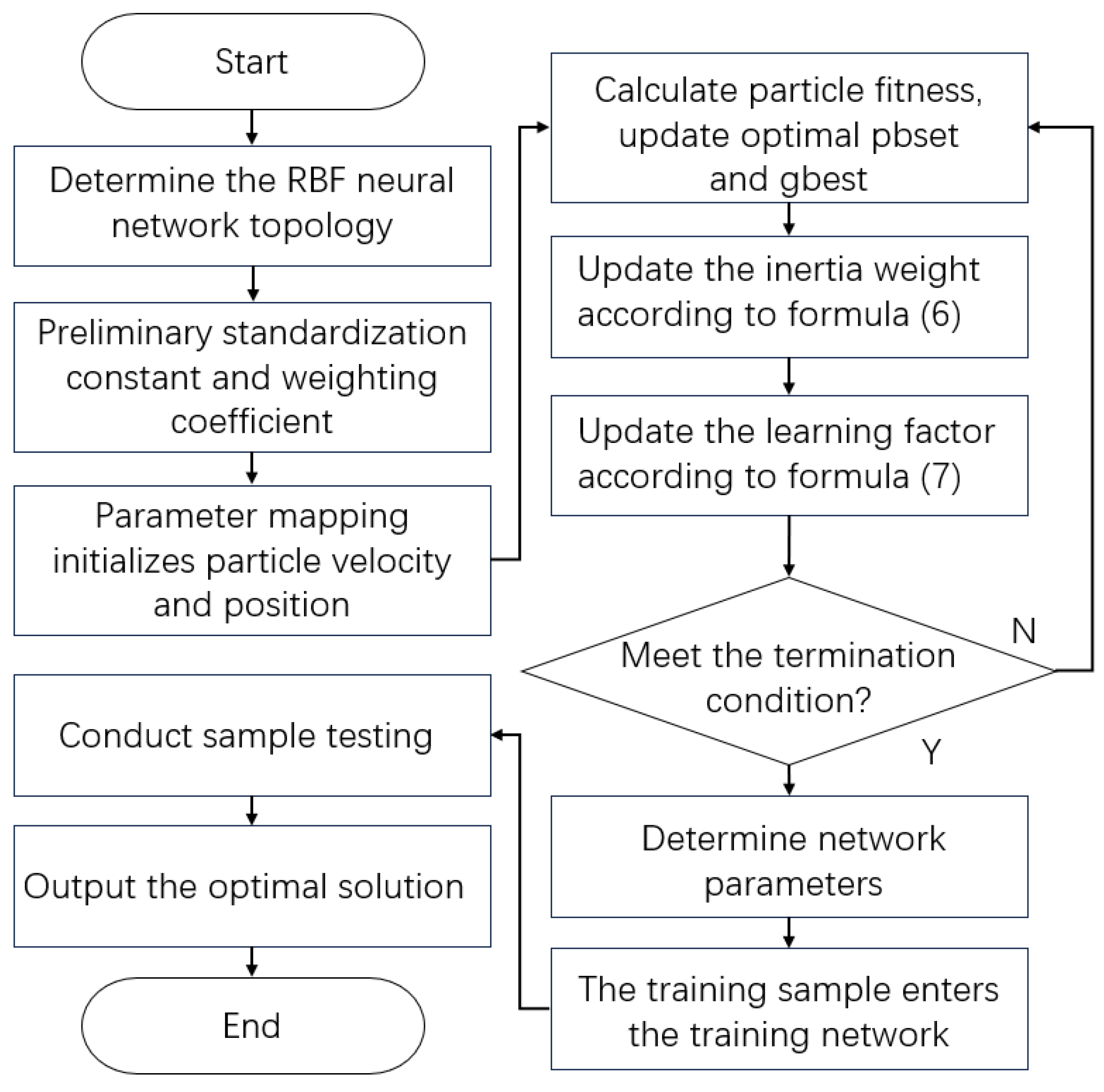
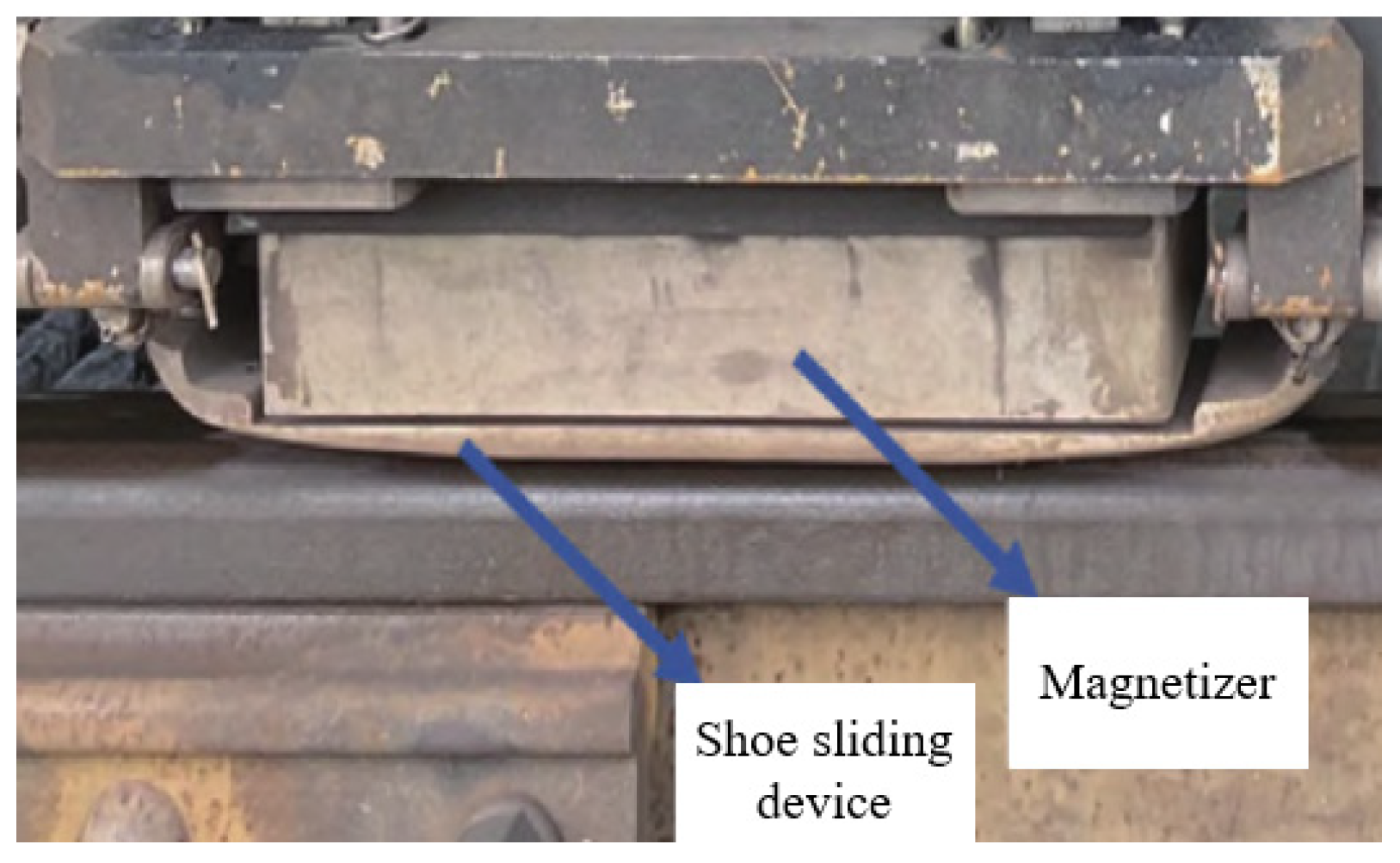
Figure 7.
Physical image of core MFL detection probe in inspection vehicle.
Disclaimer/Publisher’s Note: The statements, opinions and data contained in all publications are solely those of the individual author(s) and contributor(s) and not of MDPI and/or the editor(s). MDPI and/or the editor(s) disclaim responsibility for any injury to people or property resulting from any ideas, methods, instructions or products referred to in the content. |
© 2025 by the authors. Licensee MDPI, Basel, Switzerland. This article is an open access article distributed under the terms and conditions of the Creative Commons Attribution (CC BY) license (http://creativecommons.org/licenses/by/4.0/).
Copyright: This open access article is published under a Creative Commons CC BY 4.0 license, which permit the free download, distribution, and reuse, provided that the author and preprint are cited in any reuse.


