
Submitted:
07 June 2025
Posted:
09 June 2025
You are already at the latest version
Abstract
Asymptotic properties of the known SAIRP epidemic model are studied under stochastic perturbations, given by a combination of the white noise and Poisson's jumps. It is assumed that these stochastic perturbations are proportional to the deviation of a current state of the system under consideration from one of the system equilibria. Sufficient conditions of stability in probability for two different equilibria of the considered system are formulated via a simple linear matrix inequality (LMI) and are studied via MATLAB. Two demonstrative examples illustrate the obtained results via numerical simulation of solutions of the considered system of five nonlinear stochastic differential equations.
The research method used here can be applied to many other more complex nonlinear models in various applications.
Keywords:
equilibria
; stability in probability
; asymptotic mean square stability
; Lyapunov function
; Poisson's jumps
; Linear Matrix Inequality (LMI)
; numerical simulation
; MATLAB
MSC: 60G51; 60G52; 60H10
1. Introduction
So-called SAIRP epidemic model is described [1,2,3] by the system of five ordinary differential equations
Here it is assumed that the total population
is subdivided into five distinct classes:
- -
- susceptible individuals ();
- -
- asymptomatic infected individuals ();
- -
- active infected individuals ();
- -
- removed (including recovered and deceased) individuals ();
- -
- protected individuals ().
Besides, the total population has a variable size, the susceptible individuals become infected by contact with active infected and asymptomatic infected individuals , at a rate of infection
where represents a modification parameter for the infectiousness of the asymptomatic infected individuals . It is assumed also that all parameters of the system (1) are positive and, besides, , .
In [1,2,3] some properties of the system (1) are studied in the deterministic case, in [4] the SAIRP epidemic model is studied by the assumption that the system (1) is exposed to stochastic perturbations of the white noise type [5]. It is supposed also that these stochastic perturbations are directly proportional to the deviation of the system state from one of the two system’s equilibria, that are defined [4] by the system of five algebraic equations
with the two solutions:
1) disease-free equilibrium
where
and
2) endemic equilibrium
with
where is the basic reproduction number that is defined as follows:
Note also that, summing all equations of the system (2), we obtain for the both equilibria (3) and (4).
In contrast to [1,2,3,4], in this paper stability in probability of the both equilibria (3) and (4) of the SAIRP epidemic model (1) is studied for the first time under stochastic perturbations defined by a combination of the white noise and Poisson’s jumps. Following I.I. Gikhman and A.V. Skorokhod [5], the SAIRP model (1) becomes an object of the theory of stochastic differential equations with Poisson’s measure.
Remark 1.
Iosif Il’ich Gikhman (1918-1985) and Anatolij Vladimirovich Skorokhod (1930-2011) are two outstanding Ukrainian mathematicians, whose works have made an invaluable contribution to the development of the modern theory of stochastic processes, in particular, to the development of the theory of stochastic differential equations with Poisson’s measure. They are the authors of a large number of fundamental papers and books in the general theory of stochastic processes and in the theory of stochastic differential equations, in particular, [5,6,7,8].
2. Stochastic Perturbations
Let be a complete probability space, be a nondecreasing family of sub--algebras of , i.e., for , be the mathematical expectation with respect to the measure .
Let us suppose that the system (1) is exposed to stochastic perturbations of the type of
where and are arbitrary constants,
and are respectively -measurable and mutually independent the Wiener and the Poisson processes, , [5,6,7,8,9,10,11].
Remark 2.
Note that the Wiener processes describe continuous stochastic perturbations of the Brownian motion type, while the Poisson processes describe stochastic perturbations of the jumps type. Stability of some other models under stochastic perturbations of the type of Poisson’s jumps is studied in [9,10,11].
Let us suppose also that the stochastic perturbations (6) are directly proportional to the deviation of the system state from one of the equilibria . As a result we obtain the system of stochastic differential equations [5,8]
Note that the equilibrium of the deterministic system (1) is also the solution to the system of stochastic differential equations (7). Stochastic perturbations of this type were first proposed in [12] for the SIR epidemic model and later also for some other mathematical models in various applications (see, for instance, [13,14,15,16,17] and the references therein).
Let us note also, that unlike the present paper, where the considered system has a dimension 5, in the all mentioned previous works stochastic perturbations of the proposed type are used for systems of a dimension less than 5. This means, in particular, that the dimension of the system under consideration can in principle be increased even more.
3. Linear Approximation
Consider the nonlinear differential equation
where and the equation has a solution that is an equilibrium of differential Equation (8). Using the new variable , represent Equation (8) in the form
It is clear that stability of the zero solution to Equation (9) is equivalent to stability of the equilibrium of Equation (8).
Let , , be the Jacobian matrix of the function and , where is the Euclidean norm in . Using Taylor’s expansion in the form
and the equality , we obtain the linear approximation
of the nonlinear differential Equation (9). So, a condition for the asymptotic stability of the zero solution of the linear Equation (10) is also a condition for the local stability of the equilibrium of the initial nonlinear Equation (8).
To construct the linear approximation of the system (7) let us put
Here and everywhere below ′ is the sign of transpose.
4. Stability
Following [13], let us consider the definitions of the different types of stability for the nonlinear system (7), linear Equation (12) and the relationship between these two types of definitions (see Remark 3).
Definition 1.
Put
The solution of the system (7) is called stable in probability if for any and there exists such that satisfies the condition for any such that .
Definition 2.
The zero solution to Equation (12) is called:
-mean square stable if for each there exists a such that , , provided that ;
-asymptotically mean square stable if it is mean square stable and for each initial value such that , the solution to Equation (12) satisfies the condition .
Remark 3.
It is known [13] that sufficient conditions for asymptotic mean square stability of the zero solution of the linear part of a stochastic nonlinear system with the order of nonlinearity higher than one at the same time are sufficient conditions for stability in probability of the solution of the initial nonlinear system. So, for investigation of stability in probability of the equilibrium of the nonlinear system (7) it is enough to get conditions for asymptotic mean square stability of the zero solution of the linear Equation (12).
Remark 4.
Theorem 2.
Proof.
Using the generator (18), for the Lyapunov function , , we have
So, if the LMI (19) holds then via (20)
for some and, therefore, via Theorem 1 the zero solution to the linear stochastic differential Equation (12) is asymptotically mean square stable.
Via Remark 3 it means that the appropriate equilibrium of the nonlinear system (7) is stable in probability. The proof is completed. □
5. Numerical Simulations
5.1. Difference analogue
5.2. Examples
Here two demonstrative numerical examples are considered, where (14), (15), (16), (17) are used to calculate the matrix (13).
Example 1.
Example 2.
Remark 5.
Note that for the numerical simulation of trajectories of the Wiener processes , , in Examples 1 and 2 a special algorithm has been used, described in detail in [13] (p.29-31).
Remark 6.
6. Conclusions
Asymptotic properties of the known SAIRP epidemic model, described by a system of five nonlinear differential equations, are studied under stochastic perturbations, given by a combination of the white noise and Poisson’s jumps. It is shown that a sufficient condition of stability in probability for two equilibria of the considered system is formulated in the form of a simple linear matrix inequality (LMI), which can be easily studied via MATLAB. Two examples with numerical simulation of solutions of the considered system illustrate the obtained results.
One of the goals of the proposed paper is to attract the attention of future researchers to extension of the use of Poisson’s type stochastic perturbations in their own research, to the use of the proposed algorithm of numerical simulation of this type of perturbations together with perturbations of the type of white noise and apply this method to many other more complicated nonlinear models of higher dimensional in various applications.
Funding
This research received no external funding.
Data Availability Statement
No new data were created or analyzed in this study. Data sharing is not applicable to this article.
Conflicts of Interest
The author declares no conflicts of interest.
References
- Silva, C.J.; Cantin, G.; Cruz, C.; Fonseca-Pinto, R.; Fonseca, R.P.; Santos, E.S.; Torres, D.F.M. Complex network model for COVID-19: human behavior, pseudo-periodic solutions and multiple epidemic waves, Journal of Mathematical Analysis and Applications, 2021, Art. 125171, 23 p. [CrossRef]
- Silva, C.J.; Cruz, C.; Torresetal, D.F.M. Optimal control of the COVID-19 pandemic: controlled sanitary deconfinement in Portugal, Scientic Reports, 2021, 11(1), Art. 3451, 15 p. [CrossRef]
- Cantin, G.; Silva, C.J.; Banos, A. Mathematical analysis of a hybrid model: impacts of individual behaviors on the spreading of an epidemic, Networks & Heterogeneous Media, 2022, 17(3), 333-357. [CrossRef]
- Shaikhet, L. On stability of one mathematical model of the epidemic spread under stochastic perturbations. Biomedical Journal of Scientific & Technical Research, 2023, 53(3), 44630-44635. https://biomedres.us/pdfs/BJSTR.MS.ID.008392.pdf.
- Gikhman, I.I.; Skorokhod, A.V. Stochastic Differential Equations; Springer: Berlin/Heidelberg, Germany, 1972. [Google Scholar]
- Gikhman, I.I.; Skorokhod, A.V. The Theory of Stochastic Processes, v.I; Springer: Berlin/Heidelberg, Germany, 1974. [Google Scholar]
- Gikhman, I.I.; Skorokhod, A.V. The Theory of Stochastic Processes, v.II; Springer: Berlin/Heidelberg, Germany, 1975. [Google Scholar]
- Gikhman, I.I.; Skorokhod, A.V. The Theory of Stochastic Processes, v.III; Springer: Berlin/Heidelberg, Germany, 1979. [Google Scholar]
- Shaikhet, L. Stability of the neoclassical growth model under perturbations of the type of Poisson’s jumps: Analytical and numerical analysis. Communications in Nonlinear Science and Numerical Simulation, 2019, 72, 78–87. [Google Scholar] [CrossRef]
- Shaikhet, L. About stabilization by Poisson’s jumps for stochastic differential equations. Applied Mathematics Letters, 2024, 153 Art. 109068, 6 p. https://authors.elsevier.com/sd/article/S0893-9659(24)00088-0.
- Shaikhet, L. About stabilization of the controlled inverted pendulum under stochastic perturbations of the type of Poisson’s jumps. MDPI, Axioms, Special Issue: “Advances in Mathematical Optimal Control and Applications”, 2025, 14(1), 29, 1-14. [CrossRef]
- Beretta, E.; Kolmanovskii, V.; Shaikhet, L. Stability of epidemic model with time delays influenced by stochastic perturbations, Mathematics and Computers in Simulation, Special Issue "Delay Systems", 1998, 45(3-4), 269-277. [CrossRef]
- Shaikhet, L. Lyapunov Functionals and Stability of Stochastic Functional Differential Equations; Springer Science & Business Media: Berlin/Heidelberg, Germany, 2013. [Google Scholar] [CrossRef]
- Santonja, F-J. , Shaikhet, L. Probabilistic stability analysis of social obesity epidemic by a delayed stochastic model. Nonlinear Analysis: Real World Applications, 2014, 17, 114–125. [CrossRef]
- Shaikhet, L. Improving stability conditions for equilibria of SIR epidemic model with delay under stochastic perturbations, MDPI, Mathematics, 2020, 8(8), Art. 1302, 13 p. https://www.mdpi.com/2227-7390/8/8/1302.
- Shaikhet, L. Some generalization of the method of stability investigation for nonlinear stochastic delay differential equations. MDPI, Symmetry, 2022, 14(8), Art.1734, 13p. https://www.mdpi.com/2073-8994/14/8/1734.
- Shaikhet, L. Stability analysis of Cryptosporidiosis disease SIR model under stochastic perturbations. Communications in Mathematical Biology and Neuroscience, 2025, 2025:7, 15 p. https://scik.org/index.php/cmbn/article/view/8983.
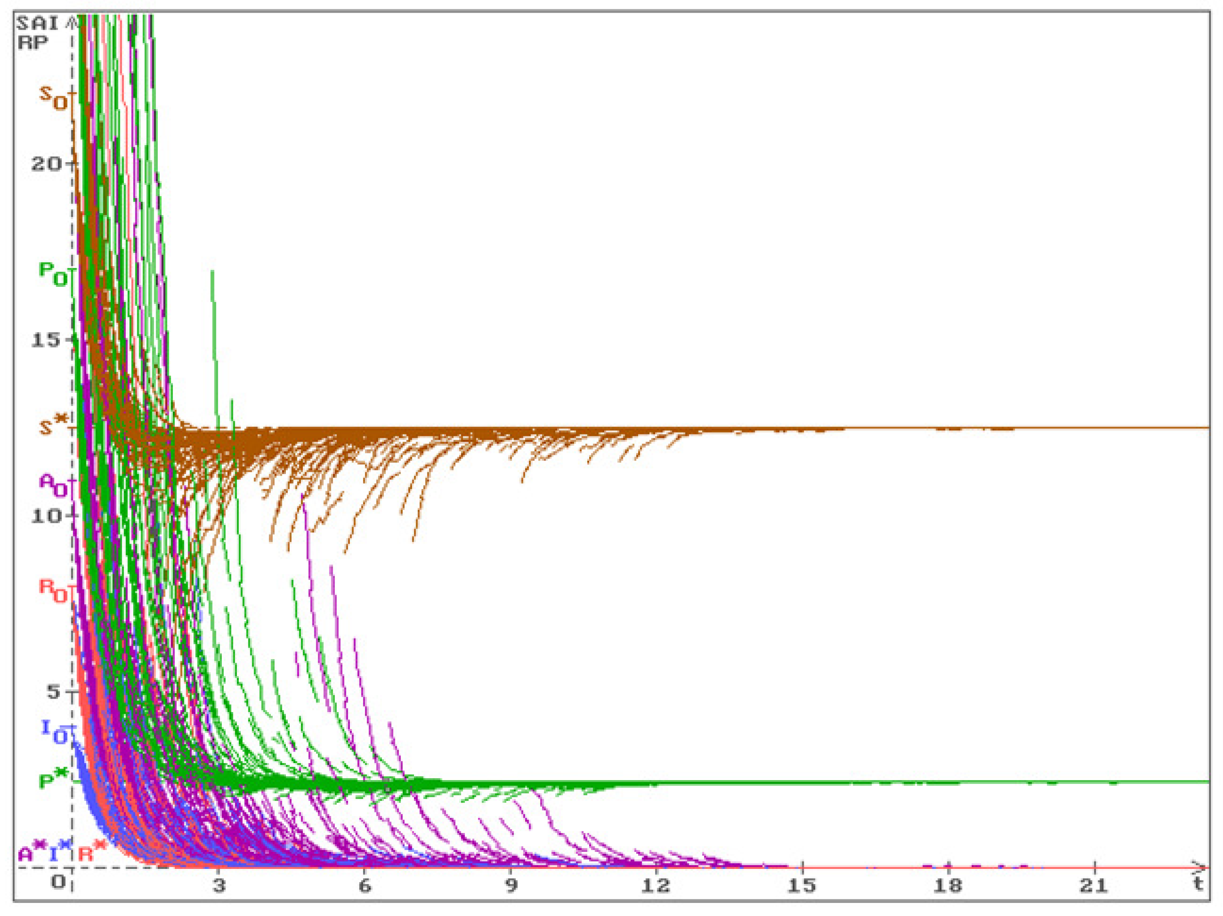
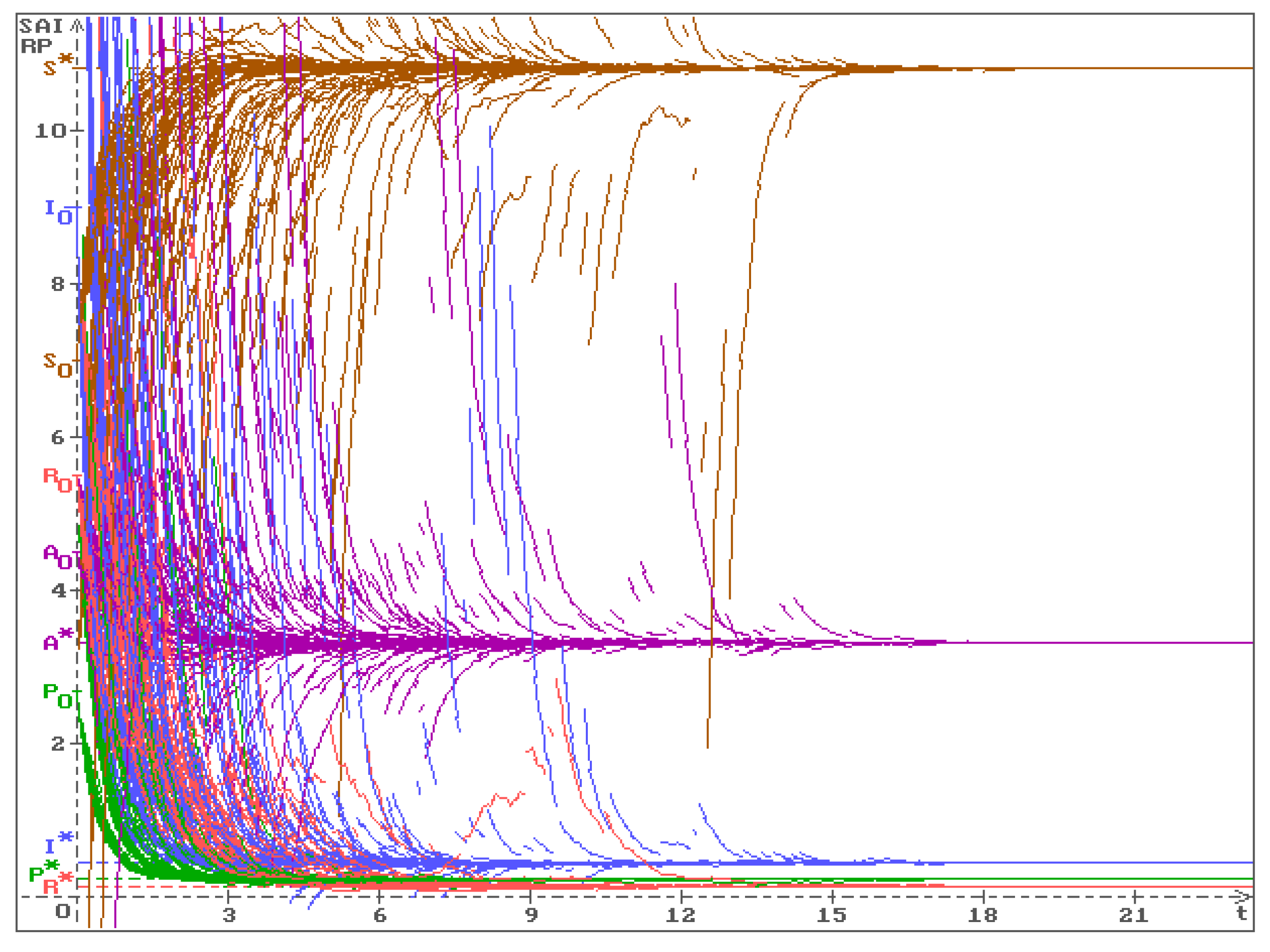
Figure 1.
Fifty trajectories of the solution of the system (7) with the parameters(23), (25), (26) converge to the stable equilibrium (24).
Disclaimer/Publisher’s Note: The statements, opinions and data contained in all publications are solely those of the individual author(s) and contributor(s) and not of MDPI and/or the editor(s). MDPI and/or the editor(s) disclaim responsibility for any injury to people or property resulting from any ideas, methods, instructions or products referred to in the content. |
© 2025 by the authors. Licensee MDPI, Basel, Switzerland. This article is an open access article distributed under the terms and conditions of the Creative Commons Attribution (CC BY) license (http://creativecommons.org/licenses/by/4.0/).
Copyright: This open access article is published under a Creative Commons CC BY 4.0 license, which permit the free download, distribution, and reuse, provided that the author and preprint are cited in any reuse.


