
Submitted:
25 April 2025
Posted:
26 April 2025
You are already at the latest version
Abstract
The escalating sophistication of cyber threats necessitates advanced threat detection in Security Operation Centers (SOCs). This study aims to enhance the capabilities of Wazuh, an open-source Security Information and Event Management (SIEM) system, by addressing its primary limitation: high false positive rates in rule-based detection. We propose integrating machine learning (ML) to improve detection accuracy and operational efficiency. The approach involves training and evaluating ML models—Random Forest (RF), Support Vector Machine (SVM), K-Nearest Neighbors (KNN), Logistic Regression, and Gaussian Naive Bayes—alongside clustering algorithms (DBSCAN, K-means, Isolation Forest) using 10-fold cross-validation. Results demonstrate that RF achieved the highest performance with an accuracy of 0.972, precision of 0.982, recall of 0.975, and F1-Score of 0.978, while DBSCAN excelled in clustering with a 91.06% accuracy and 0.0821 false positive rate. This integration significantly reduced false positives, enhancing alert management and enabling efficient real-time threat detection. The study contributes to cybersecurity by demonstrating that ML integration with Wazuh markedly improves threat detection, reduces operational overhead in SOCs, and establishes a more adaptive security framework.
Keywords:
Machine Learning
; Threat Detection
; Security Operation Center
; Supervised ML
; Unsupervised ML
; Wazuh
; Clustering Algorithms
; SIEM
; Cybersecurity
; Anomaly Detection
1. Introduction
As cyber threats evolve in both sophistication and volume, organizations must adopt advanced methodologies to bolster their security posture [1]. Wazuh, a widely adopted open-source Security Information and Event Management (SIEM) solution, plays a critical role in providing visibility into security events, log data, and potential intrusions across an organization's infrastructure. While Wazuh is a powerful tool, its effectiveness in detecting and managing threats can be hindered by several inherent limitations. Specifically, Wazuh's reliance on rule-based detection, which generates alerts based on predefined patterns, can result in a high rate of false positives. These false positives not only increase the workload for security teams but can also divert attention from actual security incidents [2].
Furthermore, Wazuh's current approach lacks the ability to adaptively learn from historical data and continuously refine its detection strategies, limiting its ability to identify evolving or previously unseen threats in real-time. In the face of large-scale data collection and analysis, Wazuh may also encounter scalability issues, particularly as organizations expand their monitoring environments [3].
This paper explores how the integration of Machine Learning (ML) can significantly enhance Wazuh’s capabilities in threat detection and management [4]. By leveraging M, Wazuh can overcome its limitations, reducing false positives, improving detection accuracy, and enabling real-time adaptive learning. ML models can help distinguish between benign events and genuine threats by learning from behavioral patterns in the data, thereby optimizing the alerting system [5], [6].
The implementation of machine learning (ML) techniques enables Wazuh to transition from a traditional rule-based approach to a more intelligent, adaptive security system capable of detecting sophisticated attacks while minimizing human intervention [7]. This paper details the technical implementation of ML models tailored for Wazuh, emphasizing data preparation, feature extraction, model training, and evaluation. Figure 1 below shows the integration process.
The integration of ML transforms Wazuh’s alerting mechanism, enhancing security monitoring operations and reducing manual effort and operational inefficiencies in Security Operation Centers (SOCs) [8]. Key areas covered include:
- ▪
- Data Preparation and Cleansing: Techniques for transforming raw security event data into structured formats suitable for ML analysis.
- ▪
- Model Training and Evaluation: Training various supervised machine learning models, including K-Nearest Neighbors, Random Forest, Naïve Bayes, Logistic Regression, and unsupervised machine learning models such as DBSCAN, K-means and Isolation Forest.
- ▪
- Model Optimization: Methods to optimize and fine-tune models to improve detection accuracy and minimize false positives.
- ▪
- Real-World Application: Best practices for integrating these models into Wazuh’s existing architecture, demonstrating their impact on alert management, false positive reduction, and overall system performance.
This study makes several significant contributions to the field of cybersecurity, particularly in the context of Security Operation Centers (SOCs) and Security Information and Event Management (SIEM) systems:
- ▪
- Enhanced Threat Detection with ML Integration: Demonstrated the successful integration of machine learning models into Wazuh, achieving a high accuracy of 0.972 with Random Forest (RF), significantly improving the system’s ability to detect sophisticated cyber threats compared to traditional rule-based methods.
- ▪
- Reduction of False Positives: Addressed Wazuh’s high false positive rates, with RF achieving a low false positive rate of 0.03 and DBSCAN clustering at 0.0821, thereby reducing alert fatigue and enhancing operational efficiency in SOCs.
- ▪
- Comprehensive Model Evaluation: Provided a thorough evaluation of multiple ML models (RF, SVM, KNN, Logistic Regression, Gaussian Naive Bayes) and clustering algorithms (DBSCAN, K-means, Isolation Forest), offering comparative insights into their performance for cybersecurity applications, with RF and DBSCAN outperforming others.
- ▪
- Improved Alert Management: Enabled more efficient real-time threat detection and alert management by streamlining the alerting mechanism, allowing SOC analysts to focus on genuine threats and reducing manual effort.
- ▪
- Framework for Adaptive Security: Established a framework for an adaptive security system by integrating ML with Wazuh, paving the way for more responsive and intelligent threat detection in dynamic cybersecurity environments.
In this paper, we have outlined how machine learning techniques can significantly enhance Wazuh’s threat detection and response capabilities. We started with an exploration of the problem statement, detailing the limitations of rule-based detection systems and the need for real-time learning and scalability. The following sections will dive deeper into the methodology of integrating ML models with Wazuh, starting with data preparation, training models, and assessing their performance in real-world security environments.
2. Related Work
The integration of machine learning (ML) and artificial intelligence (AI) into cybersecurity frameworks has been extensively explored to enhance threat detection and response in Security Operation Centers (SOCs) [9]. Hughes et al. [10] proposed a model-free reinforcement learning (RL) approach for intrusion response systems, training an RL agent in a simulated environment to mitigate complex multistage attacks while minimizing disruption to legitimate network activities. However, their method’s effectiveness was constrained by the quality and completeness of training data, potentially missing diverse attack patterns. Coscia et al. [11]developed a decision tree-based system for detecting and mitigating DoS and DDoS attacks, introducing the Anomaly2Sign algorithm to generate Suricata rules from normal and anomalous traffic in an unsupervised manner. Their decision tree model achieved an accuracy of 99.7%–99.9%, outperforming other ML classifiers, though concerns about overfitting due to unrepresentative datasets limit its practical applicability.
Advancements in Security Orchestration, Automation, and Response (SOAR) platforms further highlight the role of ML in SOCs. Kinyua and Awuah [12] examined the potential of SOAR solutions integrated with SIEM systems, arguing that AI and ML can enhance automation and operational efficiency for SOC analysts. Similarly, Islam et al. [13] introduced DecOr, a declarative API-driven orchestration framework for SOAR platforms, abstracting complexities in incident response processes to improve response accuracy, though its performance depends on the ontological knowledge base’s accuracy. Sworna et al. [13] proposed APIRO, an ML-based architecture for automatic API recommendations in SOAR solutions, achieving a Top-1 accuracy of 91.9% using data augmentation and convolutional neural networks despite data scarcity challenges.
A recent study investigated the integration of machine learning with traditional signature-based methods to enhance Network Intrusion Detection and Prevention Systems (NIDPS) against Distributed Denial-of-Service (DDoS) attacks, using Snort for traffic analysis and Wazuh for implementing a Random Forest model and active response mechanism [14]. Their Random Forest model achieved near-perfect metrics (accuracy, precision, recall, and F1-Score of 99.99%) with a training time of 18.84 seconds, enabling real-time monitoring and mitigation of DDoS attacks
However, these works often overlook open-source SIEM solutions like Wazuh and their practical deployment in resource-constrained SOCs, particularly for small and medium enterprises (SMEs). This paper contributes by demonstrating the practical application of ML in Wazuh, reducing false positives, and improving SOC efficiency through a dual approach of classification and clustering, offering a scalable solution for SMEs.
3. Materials and Methods
3.1. Design of ML-SOC Architecture
Designing an ML-SOC architecture involves addressing various challenges to ensure effective threat detection, efficient response times, and reduced false positives [12]. This section outlines a systematic approach to the design and development of the ML-SOC architecture, focusing on data collection, preprocessing, model selection, and performance evaluation.
To develop effective ML-SOC architecture, it is essential to understand the core objectives and requirements that guide its design. Table 1 below outlines the primary objectives and the corresponding requirements:
This section elaborates on the process of integrating Machine Learning (ML) to improve real-time threat detection capabilities, as shown in Figure 2. We discuss how data is prepared, pre-processed, and used for training various ML models to enhance the system's ability to identify and respond to threats effectively.
Wazuh is a powerful open-source security monitoring solution capable of providing comprehensive security analytics and visibility. In this project, Wazuh's alerting mechanisms were leveraged to collect data for further analysis. The integration included the deployment of Wazuh agents across monitored systems to capture security events, log data, and intrusion detection alerts, which were centralized for streamlined processing and analysis. The core of the Wazuh implementation included:
- ▪
- Deployment of Wazuh Agents: Installed across multiple endpoints to ensure comprehensive monitoring.
- ▪
- Centralized Data Collection: Alerts and logs were aggregated into a unified database (alerts.json), which served as the basis for the ML pipeline.
- ▪
- Rule-Based Detection: Wazuh's out-of-the-box rulesets were used to detect potential threats, generating alerts based on predefined security policies.
- ▪
- Despite its robust capabilities, Wazuh has certain limitations when used as a standalone threat detection system:
- ▪
- High Rate of False Positives: The rule-based approach can often lead to a significant number of false positives, requiring extensive manual validation.
- ▪
- Limited Real-Time Learning: Wazuh lacks the ability to adaptively learn from past data to refine detection strategies autonomously.
- ▪
- Scalability Constraints: Handling large-scale data in real-time can strain resources, impacting the performance of the detection and response processes.
- ▪
- Complex Alert Management: Managing and analyzing numerous alerts can become cumbersome, leading to potential oversight of critical threats.
These limitations underscore the need to augment Wazuh with ML models, which can enhance its detection capabilities by automating the learning process, reducing false positives, and providing more nuanced threat analyses.
Figure 2.
The proposed integration Architecture based on Machine Learning.
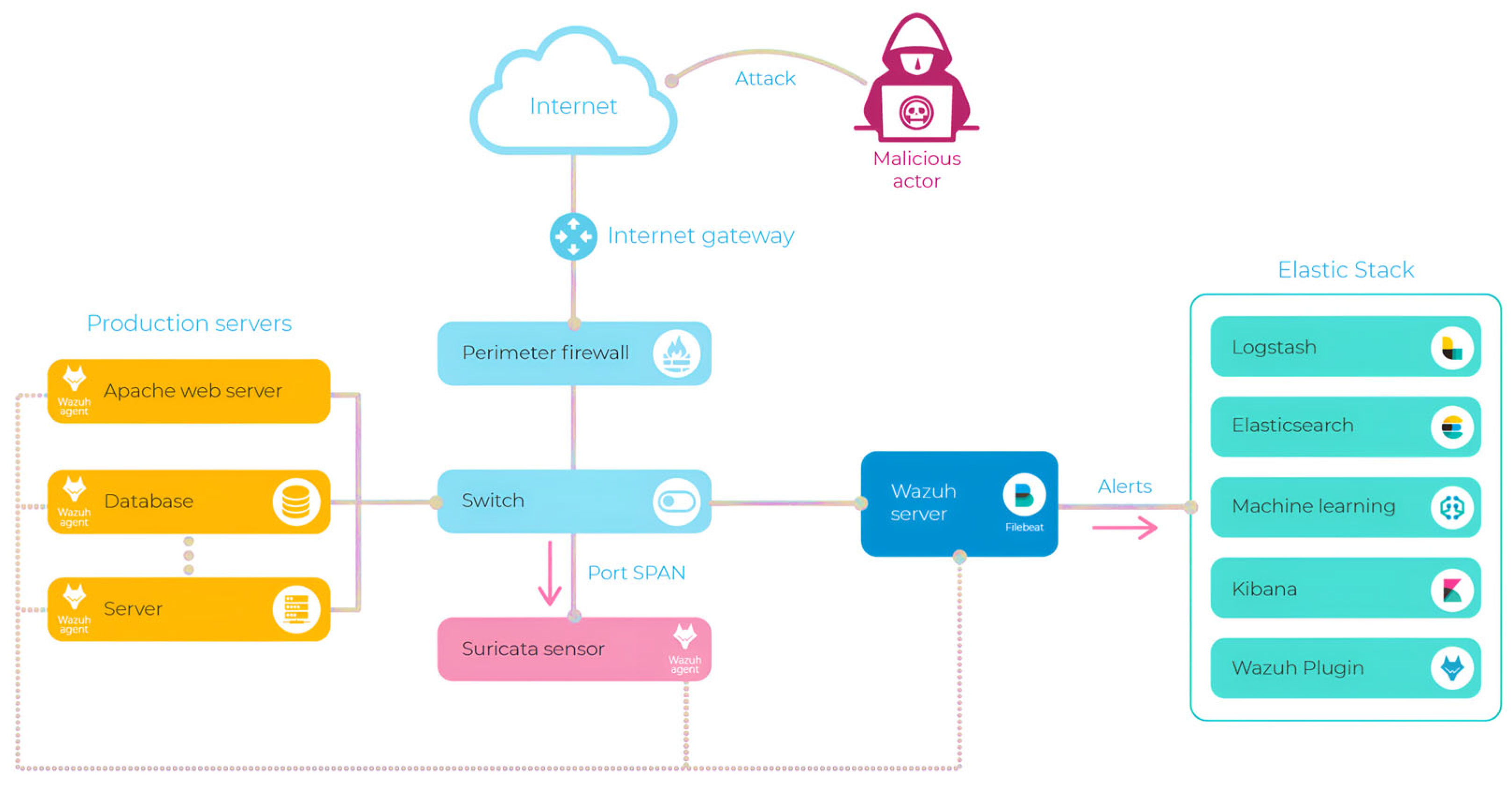
3.1. Data Collection
The system's information domain consists of log data, predominantly stored in plain text or CSV formats. Logstash is utilized to parse these logs, converting them into JSON format for structured processing. The processed logs are then archived in Elasticsearch, a NoSQL database, which serves as a core component of the ELK Stack. Furthermore, the log data is transmitted to Machine Learning (ML) models as JSON objects through API integrations, enabling advanced analytical processing. The alerts.json dataset was selected due to its wide range of data points, essential for training machine learning models aimed at identifying patterns and distinguishing between normal and anomalous behaviors [15]. This helps in developing tools that can enhance threat detection accuracy and reduce false positives.
Using the alerts.json data, machine learning models were built and refined to identify patterns indicative of false positives, with the goal of improving detection criteria and overall system accuracy. This process involved not only data collection but also its comprehensive analysis and preparation for use in model training [16].
3.2. Data Cleaning
Ensuring high data quality is crucial for the success of any machine learning model. The following steps were undertaken to cleanse the alerts.json data:
- ▪
- Exclusion of Irrelevant Data: We focused on analyzing alerts generated by monitored agents and excluded data entries related to Wazuh itself by filtering out rows where the AgentName was "wazuh".
- ▪
- Feature Extraction: Key data attributes were extracted to form a structured DataFrame. These attributes included RuleID, RuleDescription, AgentName, AgentIP, OriginalFileName, CommandLine, AlertLevel, and Timestamp. This feature engineering process transformed raw data into a structured format suitable for machine learning algorithms. Each extracted attribute provides crucial information regarding the nature and origin of alerts and their temporal context, aiding in precise threat assessment.
- ▪
- Timestamp Transformation: Timestamps were processed to extract separate date and time components (year, month, day, hour, and minute), allowing for more granular analysis of temporal trends.
- ▪
- Duplicate Removal: To prevent skewed results, duplicate entries were identified and removed, ensuring that each event in the dataset was unique and contributed independently to the analysis.
- ▪
- Handling Missing Values: Certain columns, such as OriginalFileName and CommandLine, had missing data. These gaps were addressed by assigning placeholder values such as "Unknown" to maintain dataset continuity and integrity.
- ▪
- Outlier Management: Outliers, or data points significantly different from the norm, were reviewed and addressed to avoid distortion in the model's outcomes. This step involved replacing or removing extreme values as necessary.
- ▪
- Encoding Categorical Variables: To make the dataset compatible with ML algorithms, categorical variables like AgentName, RuleDescription, Groups, OriginalFileName, and CommandLine were encoded numerically using LabelEncoder().
- ▪
- Now for a crucial step: standardising the variables involves rescaling the data so that each variable has a mean of 0 and a standard deviation of 1. This process ensures that all variables contribute equally to the analysis. By standardising, we eliminate the bias that can occur due to different scales between variables, making the model more accurate and reliable. However, we have excluded the Event Severity column from this standardisation, as it has a crucial impact and it is important not to dilute its influence through this process.
These data cleansing steps ensured that the training data was of high quality, which is essential for accurate and reliable predictions. As shown in Figure 3, a visual analysis was conducted to examine the distribution of alerts across different alert levels. This analysis helped identify which processes were most frequently associated with different alert levels, guiding security measures and preventive actions.
3.3. Data Labeling
In our approach, we utilized two distinct methods for data labeling:
- ▪
- Explicit Threat Level Labeling: Alerts were classified according to predefined threat levels to facilitate categorization and enable supervised analysis.
- ▪
- Clustering Based on Data Similarity: We employed the KMeans algorithm [17] to identify natural clusters within the data, enabling the discovery of patterns and subtle anomalies that might not be evident through explicit labels alone.
These complementary methods help define labels and classes, enhancing the accuracy and robustness of our machine learning model. We assigned labels to each alert based on its threat level, categorizing them into three distinct categories:
- ▪
- Unknown Threat (low danger level)
- ▪
- Questionable Threat (moderate danger level)
- ▪
- Dangerous Threat (high danger level)
To achieve this, we defined a mapping function to assign specific classes to the alerts based on their threat levels. After applying this function, we added a new "Class" column to the DataFrame, indicating the threat level of each alert.
3.4. Data Standardization
After thoroughly cleaning the dataset, we proceeded to separate the data into features and labels in preparation for model training. The features, represented by the variable X, were isolated by excluding the "Class" column from the dataset. Concurrently, the labels, represented by the variable y, were specifically assigned to the "Class" column.
To ensure a fair and balanced comparison across the different features, we normalized the data using the MinMaxScaler, an essential tool for scaling feature values within a specific range. This step ensures that the model can learn efficiently without being affected by variations in scale among the different input features. The normalization process implemented by the MinMaxScaler follows this formula:
(1)
Where:
▪ represents the initial value of the feature,
▪ is the minimum value of the feature in the dataset,
▪ is the maximum value of the feature in the dataset,
▪ is the resulting normalized value of the feature.
After normalizing the data, the next critical step was dividing the dataset into training and test sets. This division is essential to evaluate the model's performance on unseen data, ensuring its ability to generalize effectively. We used the train_test_split function from scikit-learn to accomplish this. For this task, 80% of the data was designated for the training set to train the model, while the remaining 20% was reserved for the test set to assess performance. This approach strikes a balance, providing enough data for robust model training and sufficient test data for a reliable performance evaluation.
To rectify the problem of class imbalance in the training dataset, we utilised SMOTE (Synthetic Minority Over-sampling Technique) . SMOTE creates synthetic cases for the minority class derived from existing examples, so successfully equilibrating the class distribution. This approach guarantees that the model is trained on a dataset with equal representation of all classes, hence augmenting its learning capacity and boosting overall accuracy. We utilised SMOTE using the fit_resample function from the imbalanced-learn package. This technique yielded a balanced training dataset, which was crucial for enhancing the model's capacity to learn from the data efficiently and generate precise predictions.
3.5. Descriptive Statistics Analysis
Descriptive statistics provide a summary of the main characteristics of the data contained in our DataFrame. Using Pandas' describe() function, we were able to obtain measures such as the mean, standard deviation, minimum, maximum and quartiles for each numerical variable in the datase. Table 2 shows a sample Encoded & Clean DATA.
3.6. Training Supervised Machine Learning Models
After dividing the data into training and test sets, the next step involves training various machine learning models on the training set and evaluating their performance on the test set. This process helps in selecting the most efficient model for our specific task. We initially used cross-validation to assess the performance of each supervised learning model. A 10-fold cross-validation with the KFold method (KFold(n_splits=10)) was applied to estimate the mean accuracy of the model over different subsets of the training data.
3.5.1. K-Nearest Neighbors (KNN) Classifier
The K-Nearest Neighbours (KNN) [18]model is a supervised learning technique employed for classification and regression tasks. It forecasts the label of a data point by referencing the labels of its nearest neighbours in the feature space, utilising the idea that analogous data points aggregate together.
Steps:
- ▪
- Defined a parameter grid (param_grid_knn) with n_neighbors ranging from 1 to 100 and used both Euclidean and Manhattan distance metrics.
- ▪
- Employed GridSearchCV for hyperparameter tuning using 10-fold cross-validation.
- ▪
- Trained the model on the training set (X_train, y_train).
- ▪
- Evaluated the best model on the test set (X_test, y_test) to provide an unbiased estimate of its performance.
- ▪
- Used the best model to make predictions on the test set, obtaining the predicted labels (y_predict_knn).
3.5.2. Random Forest Classifier (RF)
The Random Forest Classifier (RF) [19]is a widely used ensemble learning method that aggregates multiple decision trees to enhance predictive performance. It reduces overfitting and improves generalization by averaging or taking a majority vote from several decision trees trained on different subsets of the training data.
Steps:
- ▪
- Trained an ExtraTrees classifier to perform feature selection using SelectFromModel.
- ▪
- Trained the RFC model with n_estimators=100 using the selected features.
- ▪
- Used the trained RFC model to make predictions on the test set.
3.5.3. Naïve Bayes Classifier
The Naïve Bayes classifier [20], founded on Bayes' theorem, presupposes conditional independence among features, contingent upon the class label. It is useful for text classification and other data types when the assumption of feature independence is justifiable.
Steps:
- ▪
- Initialized the Gaussian Naïve Bayes classifier.
- ▪
- Defined a parameter grid for hyperparameter tuning, focusing on the var_smoothing parameter.
- ▪
- Trained the model with the best hyperparameters.
- ▪
- Evaluated the model’s performance on the test set.
3.5.4. Logistic Regression
Logistic regression is a generalized linear model used for classification tasks and is valued for its simplicity and ability to provide interpretable results.
Steps:
- ▪
- Initialized the logistic regression model and defined a parameter grid to optimize the C (regularization strength) and penalty settings.
- ▪
- Used GridSearchCV to find the best hyperparameters.
- ▪
- Trained the model using the optimal configuration and evaluated its performance on the test set.
3.7. Training Unsupervised ML Techniques
In this section, we implement a preprocessing technique to improve the accuracy of clustering in a safety dataset. accuracy of clustering in a safety dataset. Clustering is a commonly used method commonly used to identify patterns and anomalies in data; however, it requires that all requires all features to be on the same scale to avoid favouring those with larger those with higher values. Standardisation, which adjusts the data so that it has mean of zero and a standard deviation of one, ensures that each feature contributes equally to the equally to the clustering algorithm. One of the key features of our dataset, Event Severity, represents the criticality of events, where higher values indicate more serious security incidents. To preserve the influence of this characteristic, we have chosen not to not standardise it, in order to maintain the weight of high-severity events in the clustering process. This method makes it possible to obtain more accurate clustering by ensuring that critical events are given the appropriate weight when identifying patterns or anomalies. anomalies. The following code shows the steps taken to scale the other features and combine them with Severity. combined with weighted Event Severity, to ensure balanced and relevant clustering results. clustering results. Alrogithm shows the steps taken to scale the other characteristics and combine them with the weighted Event Severity, to ensure balanced and relevant clustering results.
Algorithm 1: Preprocess Data for Clustering with Severity
Input: Data (a dataset with features including 'Event Severity')
Output: ScaledData (a dataset with standardized features and original 'Event Severity')
1. // Select features for standardization, excluding 'Event Severity'
2. FeaturesToStandardize ← Data.DropColumn('Event Severity')
3. // Standardize the selected features
4. Scaler ← InitializeStandardScaler()
5. ScaledFeatures ← Scaler.FitTransform(FeaturesToStandardize)
6. // Combine the standardized features with the original 'Event Severity'
7. ScaledData ← CreateDataFrame(ScaledFeatures, Columns ← FeaturesToStandardize.Columns)
8. ScaledData['Event Severity'] ← Data['Event Severity']
9. Return ScaledData
3.7.1. K-means
Before applying the K-Means clustering algorithm, it is essential to determine the optimal number of clusters, denoted as k, as this parameter has a direct impact on the clustering quality. Choosing an inappropriate number of clusters can lead to suboptimal results, either by overfitting or underfitting the data structure.
Overfitting occurs when an excessive number of clusters is specified, resulting in the model capturing noise and minor fluctuations in the data, thereby losing generalizability. Conversely, underfitting happens when too few clusters are used, which can cause important structures or natural groupings in the data to be overlooked.
To systematically determine the appropriate value for k, two well-established techniques were applied: the Silhouette Score and the Elbow Method. The Silhouette Score provides a quantitative assessment of clustering quality by measuring how similar a data point is to its own cluster compared to other clusters. Scores range from -1 to +1, with higher values indicating that clusters are well-separated and internally cohesive. The silhouette analysis revealed that the clustering structure is most distinct when k = 2, suggesting this value provides the clearest separation between groups.
To complement this analysis, the Elbow Method was also utilized. This approach involves plotting the within-cluster sum of squares (WCSS) against various values of k. Initially, as k increases, the WCSS decreases sharply due to improved fit. However, after a certain point, the rate of decrease slows down significantly, forming an "elbow" in the plot. This inflection point marks a balance between minimizing intra-cluster distance and maintaining model simplicity, serving as a practical guide for selecting k.
Based on the results of the Silhouette Score, the number of clusters was set to 2. The K-Means model was initialized with this value of k, and a fixed random_state of 42 was specified to ensure reproducibility of the clustering results. The model was then trained on the standardized dataset, allowing it to iteratively partition the data into the defined number of clusters by minimizing intra-cluster variance. Upon training, cluster assignments were generated for each data point. These assignments, which indicate the closest cluster centroid for each observation, were added to the dataset in a new column labeled cluster.
To assess the distribution of data points within their respective clusters, the algorithm computed the Euclidean distances between each point and all cluster centroids using the transform method. The minimum of these distances—representing the proximity to the nearest cluster center—was stored in a new column named distance_to_centroid.
To detect potential anomalies, a threshold was derived based on the 99.7th percentile of the distance distribution. Any point whose distance exceeded this threshold was considered an outlier, as it significantly deviated from the typical intra-cluster distance pattern. These points were flagged in a new column named anomaly.
This clustering-based anomaly detection approach proved effective in identifying outliers. By focusing on the uppermost 0.3% of data points in terms of distance to the nearest centroid, the model isolated observations that deviated notably from the core structure of the data, thereby enabling more targeted investigations into these atypical instances.
3.7.2. Isolation Forest
Isolation Forest is an unsupervised learning algorithm specifically designed for anomaly detection [21]. Unlike clustering-based techniques, it does not attempt to model normal instances but rather isolates anomalies directly. The underlying assumption is that anomalies are few and different, making them easier to separate from the rest of the data.
The algorithm constructs multiple isolation trees by randomly selecting a feature and a split value. Since anomalies are rare and often exhibit attribute values that differ significantly from normal observations, they are typically isolated closer to the root of the tree, resulting in shorter path lengths. Conversely, normal points usually require more partitions to be isolated, leading to longer path lengths.
The Isolation Forest model was initialized with a contamination parameter set to 0.01, indicating that approximately 1% of the dataset is expected to be anomalous. This value influences the threshold used for anomaly detection. To ensure consistent and reproducible results, the random seed was fixed using a specific value.
Once initialized, the model was trained on the preprocessed dataset. During this process, it assigned a prediction label to each data point: -1 for anomalies and 1 for normal observations. These predictions were stored in a dedicated column labeled anomaly in the dataset, facilitating the identification of unusual behaviors.
After training and prediction, the dataset was filtered to retain only those instances labeled as anomalies. These entries, identified as having a significantly shorter average path length across the isolation trees, were extracted and compiled into a separate dataset for further analysis.
This method allowed for efficient detection of outliers based on their isolation characteristics, without requiring any assumptions about the underlying distribution of the data. As shown in Figure 4, the results demonstrated the effectiveness of Isolation Forest in identifying subtle and potentially high-impact anomalies that may escape traditional clustering-based approaches.
3.7.2. DBSCAN
DBSCAN (Density-Based Spatial Clustering of Applications with Noise) is an unsupervised clustering algorithm that identifies dense regions in data and treats low-density regions as anomalies or noise [22]. It is particularly effective for discovering clusters of arbitrary shape and for distinguishing outliers in datasets with varying densities., The algorithm relies on two key parameters:
- ▪
- eps (epsilon): the maximum distance between two samples for them to be considered neighbors.
- ▪
- min_samples: the minimum number of neighboring points required to form a dense region.
In this study, the parameters were set to eps = 0.3 and min_samples = 3. This configuration means that any data point must have at least two other points within a 0.3-unit radius to be considered part of a cluster. Otherwise, it is labeled as noise.
Once initialized, the DBSCAN algorithm was applied to the preprocessed dataset. It assigned cluster labels to each data point. Points that could not be assigned to any cluster were marked with the label -1, signifying that they are outliers or anomalies.
To identify these anomalies, the assigned labels were analyzed, and all points labeled as -1 were extracted. These instances were flagged in a new column labeled anomaly and isolated in a separate dataset for further inspection.
As shown in Figure 5. The results of the DBSCAN algorithm highlighted specific data points as noise, which did not belong to any dense region. This unsupervised approach enabled the detection of anomalies without prior knowledge of the data structure or assumptions about distribution. Compared to other methods, DBSCAN is especially robust in datasets where clusters may vary in shape and size, making it a valuable tool for identifying complex patterns and outliers.
4. Results and Discussion
To discuss performance metrics based on the provided code snippet, we must understand how each metric evaluates a machine learning model’s performance, especially in classification tasks. The following are the performance metrics with their explanations and corresponding equations:

Table 3.
performance metrics with their explanations and corresponding equations.
| Metric | Description | Calculation |
| True Positive Rate (TPR) | Sensitivity or Recall: Fraction of actual positives correctly classified as positive. | |
| False Positive Rate (TNR) | Specificity: Fraction of actual negatives incorrectly classified as positive. | |
| Precision | Fraction of positive predictions that were actually positive. | |
| Accuracy | Fraction of instances correctly classified by the algorithm. | |
| Recall | The percentage of correct positive predictions out of all thepositive values. | |
| F1-Score | This is the weighted harmonic mean of precision and recall. | |
| Confusion matrix | It shows the number of correct predictions (TP and TN) and incorrect predictions (FP and FN). |
4.1. Supeervised ML Techniques
Table 4 provided outlines the comparative performance of five machine learning models (Random Forest, K-Nearest Neighbors, Logistic Regression, Gaussian Naive Bayes, and Support Vector Machine) using common evaluation metrics: accuracy, precision, true positive, true negative, false positive, false negative, true positive rate (TPR), and false positive rate (FPR). Each metric provides insight into different aspects of the models' performances on a classification task.
The Random Forest Classifier (RFC) emerged as the top-performing model, achieving an accuracy of 0.972, as shown in Table 4. RFC also demonstrated exceptional precision (0.982) and recall (0.975), resulting in a corrected F1-Score of 0.978, reflecting its ability to effectively balance the minimization of false positives and false negatives. The model’s low false positive rate (FPR) of 0.03, coupled with a high true positive rate (TPR) of 0.98, underscores its reliability in avoiding false alarms while accurately detecting true threats. This performance highlights RFC’s robustness in handling complex, high-dimensional data structures, making it an ideal choice for high-stakes cybersecurity scenarios where minimizing false positives is critical, such as in threat detection systems.
The Support Vector Machine (SVM) followed closely, with an accuracy of 0.965, precision of 0.970, recall of 0.971, and a corrected F1-Score of 0.971 (Table 6.6, Figure X). SVM’s performance reflects its strength in handling high-dimensional data with clear boundaries, as evidenced by its competitive TPR of 0.96 and FPR of 0.04. Although its TPR is slightly lower than RFC’s, SVM excels in recognizing true positive cases, making it a strong contender for cybersecurity applications where data classes are well-separated. However, its minor shortfall in TPR compared to RFC suggests that SVM might miss some true threats in scenarios with overlapping or highly complex data distributions. Nonetheless, SVM remains a viable alternative to RFC, particularly in tasks requiring efficient classification in high-dimensional spaces.
K-Nearest Neighbors (KNN) achieved an accuracy of 0.963, with a precision of 0.960, recall of 0.961, and a corrected F1-Score of 0.960 (Table 6.6, Figure X). While KNN demonstrates robust performance, its FPR of 0.04 is slightly higher than RFC and SVM, indicating a potential for more false alarms. KNN is well-suited for smaller datasets with distinct patterns, as it relies on proximity-based classification. However, its performance can degrade in higher-dimensional spaces due to the curse of dimensionality, which may explain its slightly lower metrics compared to RFC and SVM. Despite this, KNN offers a balanced trade-off between precision and recall, making it a reliable general-purpose model for cybersecurity classification tasks.
Logistic Regression delivered a solid performance with an accuracy of 0.939, precision of 0.951, recall of 0.941, and a corrected F1-Score of 0.946 (Table 6.6, Figure X). As a linear model, Logistic Regression maintains high precision and recall, but it falls slightly behind non-linear models like RFC and SVM in overall performance. Its TPR of 0.94 and FPR of 0.05 indicate reliable detection of true threats with a moderate rate of false alarms. Logistic Regression is advantageous for problems with linear decision boundaries and serves as an effective baseline for classification tasks in cybersecurity. However, its performance may be limited when dealing with complex, non-linear relationships in the data, which are common in real-world cybersecurity datasets.
Gaussian Naive Bayes, despite its simplicity, achieved an accuracy of 0.927, the lowest among the evaluated models, with a precision of 0.923, recall of 0.911, and a corrected F1-Score of 0.917 (Figure 6). This performance is attributed to its assumption of feature independence, which often does not hold in complex cybersecurity datasets. The model’s higher FPR (0.08) and lower TPR (0.90) compared to the other models suggest it generates more false positives and misses some true threats, making it less suitable for applications requiring minimal false alarms. Nevertheless, Gaussian Naive Bayes remains effective for straightforward datasets with minimal inter-feature dependencies, offering reasonable precision and recall for simpler classification tasks.
Overall, the Random Forest Classifier stands out as the best model, with the highest accuracy, precision, recall, and F1-Score, alongside the lowest FPR, proving its effectiveness in complex and diverse cybersecurity classification tasks. SVM also performed exceptionally well, offering a strong alternative for scenarios where linear decision boundaries are insufficient, and its high recall makes it particularly adept at identifying true threats. KNN and Logistic Regression provide balanced trade-offs, with KNN excelling in smaller, distinct datasets and Logistic Regression serving as a reliable baseline for linear problems. Gaussian Naive Bayes, while fast and simple, is best suited for simpler data structures with independent features, as its performance lags in more complex scenarios.
4.2. Unsupeervised ML Techniques
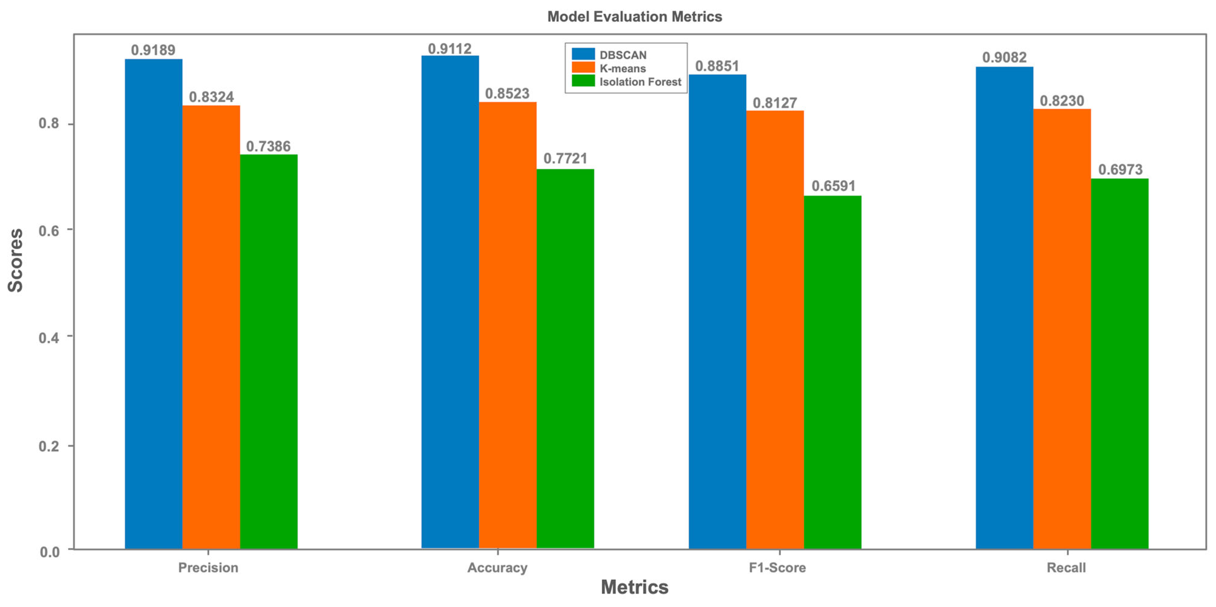
The evaluation metrics (Precision, Recall, F1-score and Accuracy) confirm the observations made from the confusion matrices. DBSCAN obtains the best scores in all metrics, underlining its robustness in detecting anomalies. K-means shows average results, while Isolation Forest, despite its detection capabilities, ranks last. The bar charts of the evaluation metrics highlight the superiority of DBSCAN, positioning this algorithm as the preferred choice for our use case. This analysis shows that DBSCAN is the most effective at minimising misclassification and detecting anomalies compared to the other algorithms in this simulation.
Figure 7.
Unsupervised ML techniques Scores.
- ▪
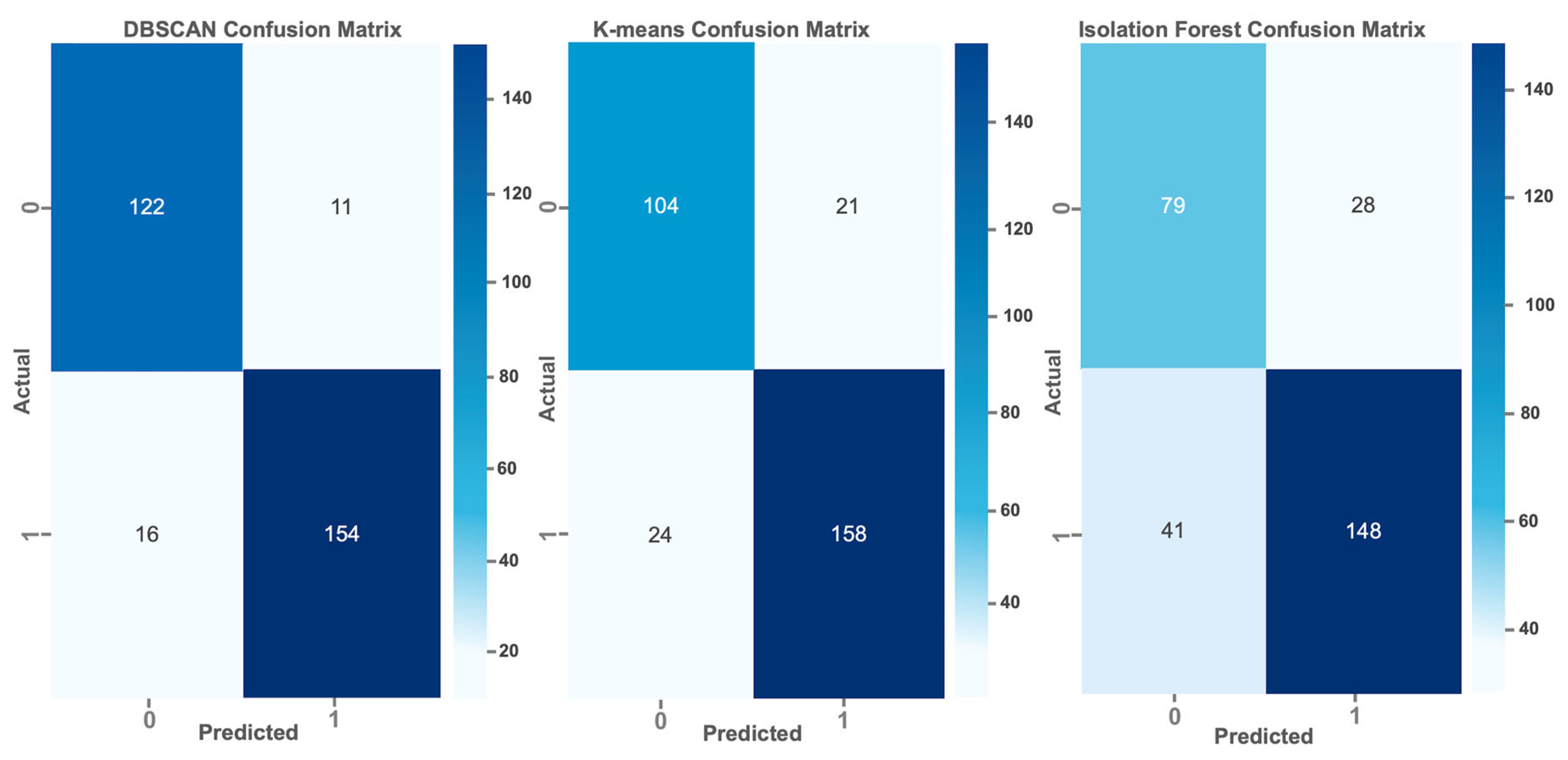
- Confusion Matrix
We compared the performance of three anomaly detection algorithms DBSCAN, K-means and Isolation Forest using sample logs to illustrate their relative effectiveness. Confusion matrices were designed to reflect the accuracy levels of the algorithms. The results show that DBSCAN outperforms both K-means and Isolation Forest. DBSCAN outperformed with a higher number of True Positives (TP) and a lower number of False Positives (FP), indicating its effectiveness in correctly identifying anomalies while minimising false alarms. In comparison, K-means shows an intermediate performance with moderate levels of TP and FP, while Isolation Forest, although functional, shows the weakest performance of the three, with fewer TP and more FP.
Figure 8.
Confusion Matrix.
5. Conclusions
The integration of machine learning models into the Wazuh environment has significantly enhanced its cybersecurity capabilities, as evidenced by the performance metrics in Figure X ("Model Evaluation Metrics"). The Random Forest Classifier (RFC) achieved the highest accuracy of 0.972, with a precision of 0.982, recall of 0.975, and a corrected F1-Score of 0.978, demonstrating its ability to minimize false positives and negatives effectively. Support Vector Machine (SVM) followed closely with an accuracy of 0.965, precision of 0.970, recall of 0.971, and an F1-Score of 0.971, excelling in high-dimensional data scenarios. K-Nearest Neighbors (KNN) recorded an accuracy of 0.963, with a precision of 0.960, recall of 0.961, and an F1-Score of 0.960, while Logistic Regression achieved an accuracy of 0.939, precision of 0.951, recall of 0.941, and an F1-Score of 0.946. Gaussian Naive Bayes, with an accuracy of 0.927, precision of 0.923, recall of 0.911, and an F1-Score of 0.917, performed the least effectively due to its feature independence assumption.
This deployment addressed the Wazuh platform’s high false positive rate, which previously overburdened security analysts and delayed responses. The reduction in false positives, particularly with RFC and SVM, streamlined alert management, enabling analysts to focus on genuine threats and improving operational efficiency. Automation reduced manual workloads, freeing resources for strategic tasks like threat hunting. In conclusion, integrating machine learning into Wazuh significantly improves threat detection and response, with RFC and SVM leading in performance. This study underscores the potential of machine learning to enhance cybersecurity infrastructures, suggesting future exploration of Generative AI for further optimization.
Future work could explore integrating Generative AI to augment datasets with synthetic cyber threats, enhancing model robustness. Additionally, incorporating clustering metrics like Silhouette Score or Adjusted Rand Index could better evaluate unsupervised methods. Exploring deep learning models or hybrid approaches may further improve detection of complex threats, while real-time adaptation to evolving attack patterns could strengthen the system’s responsiveness in dynamic cybersecurity environments.
Author Contributions
Conceptualization, S.A.C., Y.M. and N.G.; methodology, S.A.C. Y.M. and M.Z.; software, S.A.C.; validation, M.Z., Y.M. and N.G.; formal analysis, S.A.C.; investigation, S.A.C.; resources, S.A.C.; data curation, S.A.C. and M.Z.; writing—original draft preparation, S.A.C. and Y.M.; writing—review and editing, S.A.C., Y.M., M.Z. and N.G.; visualization, S.A.C.; supervision, Y.M. and S.A.C.; project administration, Y.M.; funding acquisition, M.Z. and Y.M. All authors have read and agreed to the published version of the manuscript.
Funding
Please add: This research received no external funding.
Data Availability Statement
The dataset is available upon request from the authors
Acknowledgments
We express our gratitude to LaSTI Laboratory of Sultan Moulay Slimane University, Beni Mellal, Morocco, for supporting this work.
Conflicts of Interest
The authors declare no conflicts of interest
References
- S. A. Chamkar, Y. Maleh, and N. Gherabi, “Security Operations Centers: Use Case Best Practices, Coverage, and Gap Analysis Based on MITRE Adversarial Tactics, Techniques, and Common Knowledge,”. Journal of Cybersecurity and Privacy, 2024, 4, 777–793. [CrossRef]
- H. Mokalled, R. Catelli, V. Casola, D. Debertol, E. Meda, and R. Zunino, “The Applicability of a SIEM Solution: Requirements and Evaluation. BT - 28th IEEE International Conference on Enabling Technologies: Infrastructure for Collaborative Enterprises, WETICE 2019, Naples, Italy, June 12-14, 2019,” 2019. [CrossRef]
- M. Sheeraz et al., “Effective security monitoring using efficient SIEM architecture,” Hum.-Centric Comput. Inf. Sci, vol. 13, pp. 1–18, 2023.
- Y. Maleh, “Machine Learning Techniques for IoT Intrusions Detection in Aerospace Cyber-Physical Systems BT - Machine Learning and Data Mining in Aerospace Technology,” A. E. Hassanien, A. Darwish, and H. El-Askary, Eds., Cham: Springer International Publishing, 2020, pp. 205–232. [CrossRef]
- M. Belaissaoui, Y. Qasmaoui, S. Mounir, and Y. Maleh, “Cybersecurity-Based Machine Learning for Cyber-Physical Systems,” in Security Engineering for Embedded and Cyber-Physical Systems, 2022, pp. 161–191. [CrossRef]
- S. E. Hajla, E. Mahfoud, Y. Maleh, and S. Mounir, “Attack and anomaly detection in IoT Networks using machine learning approaches,” in Proceedings - 10th International Conference on Wireless Networks and Mobile Communications, WINCOM 2023, 2023. [CrossRef]
- S. A. Chamkar, Y. Maleh, and N. Gherabi, “THE HUMAN FACTOR CAPABILITIES IN SECURITY OPERATION CENTER (SOC),” EDPACS, vol. 66, no. 1, pp. 1–14, 2022. [CrossRef]
- A. A. Mughal, “Building and securing the modern security operations center (soc),” International Journal of Business Intelligence and Big Data Analytics, vol. 5, no. 1, pp. 1–15, 2022.
- M. Khayat, E. Barka, M. A. Serhani, F. Sallabi, K. Shuaib, and H. M. Khater, “Empowering Security Operation Center with Artificial Intelligence and Machine Learning–A Systematic Literature Review,” IEEE Access, 2025.
- K. Hughes, K. McLaughlin, and S. Sezer, “Dynamic countermeasure knowledge for intrusion response systems,” in 2020 31st Irish Signals and Systems Conference (ISSC), IEEE, 2020, pp. 1–6.
- A. Coscia, V. Dentamaro, S. Galantucci, A. Maci, and G. Pirlo, “Automatic decision tree-based NIDPS ruleset generation for DoS/DDoS attacks,” Journal of Information Security and Applications, vol. 82, p. 103736, 2024.
- J. Kinyua and L. Awuah, “AI/ML in Security Orchestration, Automation and Response: Future Research Directions.,” Intelligent Automation & Soft Computing, vol. 28, no. 2, 2021.
- Z. T. Sworna, C. Islam, and M. A. Babar, “Apiro: A framework for automated security tools api recommendation,” ACM Transactions on Software Engineering and Methodology, vol. 32, no. 1, pp. 1–42, 2023.
- O. Toyin et al., “Intelligent Network Intrusion Detection and Prevention System (NIDPS): A Machine Learning and Network Security,” in 2024 IEEE 5th International Conference on Electro-Computing Technologies for Humanity (NIGERCON), 2024, pp. 1–6. [CrossRef]
- V. Önal, H. Arslan, and Y. Görmez, “Machine Learning and Event-Based User and Entity Behavior Analysis,” in 2024 32nd Signal Processing and Communications Applications Conference (SIU), IEEE, 2024, pp. 1–4.
- B. Karampudi, D. M. Phanideep, V. M. K. Reddy, N. Subhashini, and S. Muthulakshmi, “Malware Analysis Using Machine Learning,” in Intelligent Systems Design and Applications, A. Abraham, S. Pllana, G. Casalino, K. Ma, and A. Bajaj, Eds., Cham: Springer Nature Switzerland, 2023, pp. 281–290.
- M. Silic, G. Delac, and S. Srbljic, “Prediction of Atomic Web Services Reliability Based on K-means Clustering,” in Proceedings of the 2013 9th Joint Meeting on Foundations of Software Engineering, in ESEC/FSE 2013. New York, NY, USA: ACM, 2013, pp. 70–80. [CrossRef]
- J. Laaksonen and E. Oja, “Classification with learning k-nearest neighbors,” in Neural Networks, 1996., IEEE International Conference on, 1996, pp. 1480–1483 vol.3. [CrossRef]
- L. Breiman, “Random forests. Machine learning,” pp. 1–33, 2001. [CrossRef]
- I. Rish, “An empirical study of the naive Bayes classifier,” In IJCAI 2001 workshop on empirical methods in artificial intelligence, vol. 3, no. 22, pp. 41–46, 2001.
- F. T. Liu, K. M. Ting, and Z.-H. Zhou, “Isolation forest,” in 2008 eighth ieee international conference on data mining, IEEE, 2008, pp. 413–422.
- E. Schubert, J. Sander, M. Ester, H. P. Kriegel, and X. Xu, “DBSCAN revisited, revisited: why and how you should (still) use DBSCAN,” ACM Transactions on Database Systems (TODS), vol. 42, no. 3, pp. 1–21, 2017.
Figure 1.
ML Integration process.
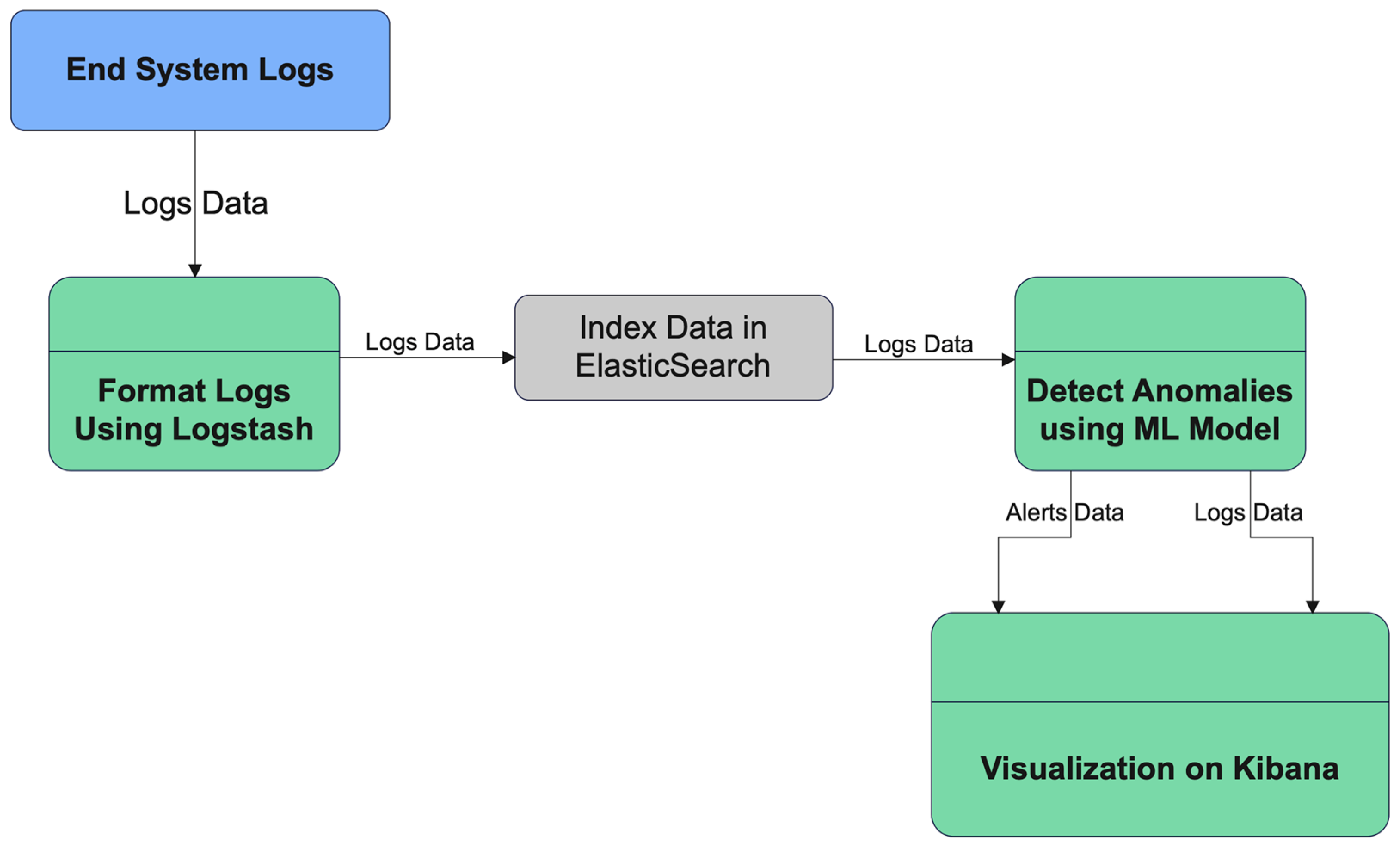
Figure 3.
Visualization of Processes Based on Alert Levels.
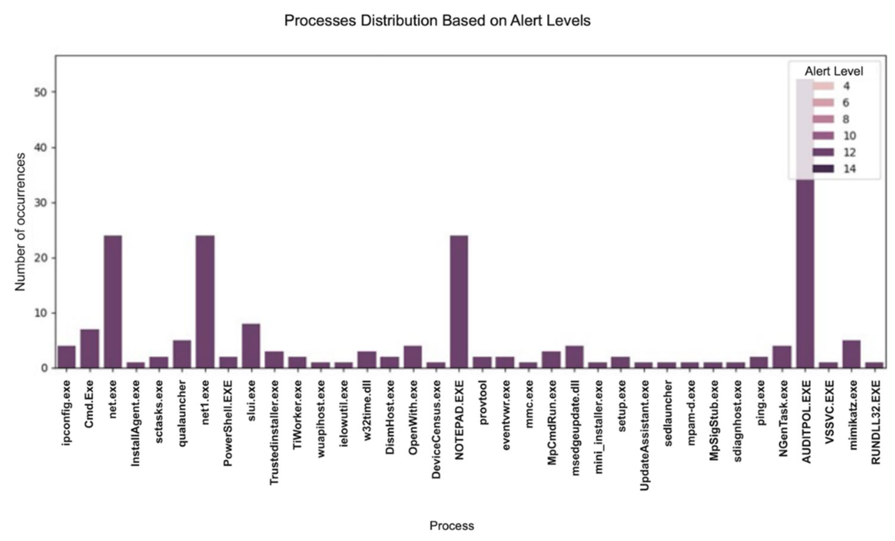
Figure 4.
Isolation Forest Results
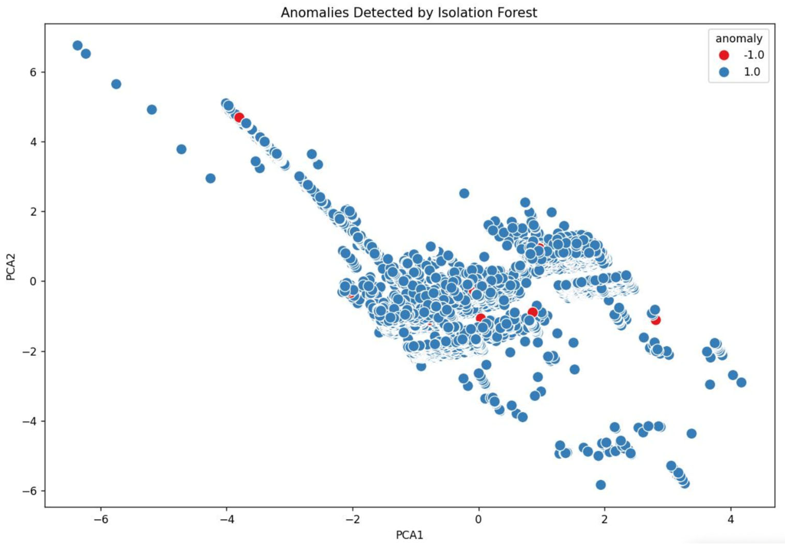
Figure 5.
DBSCAN Results
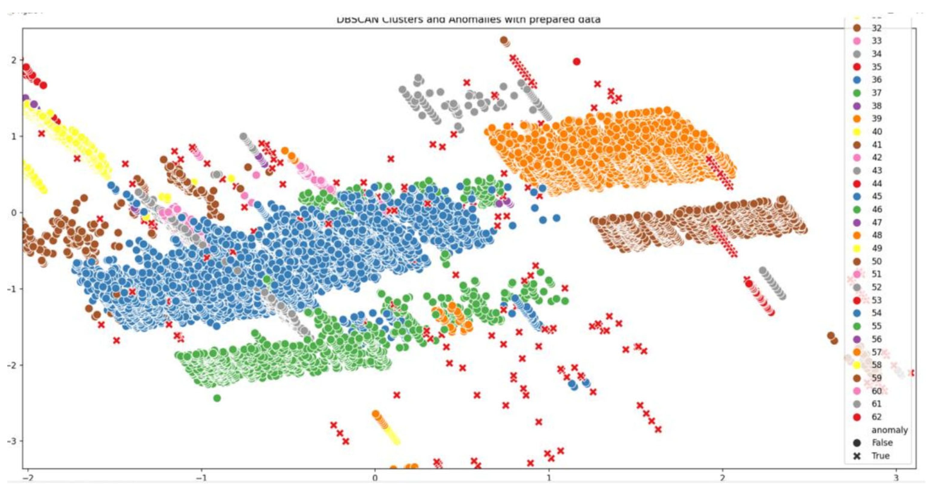
Figure 6.
Supervised ML techniques Scores.
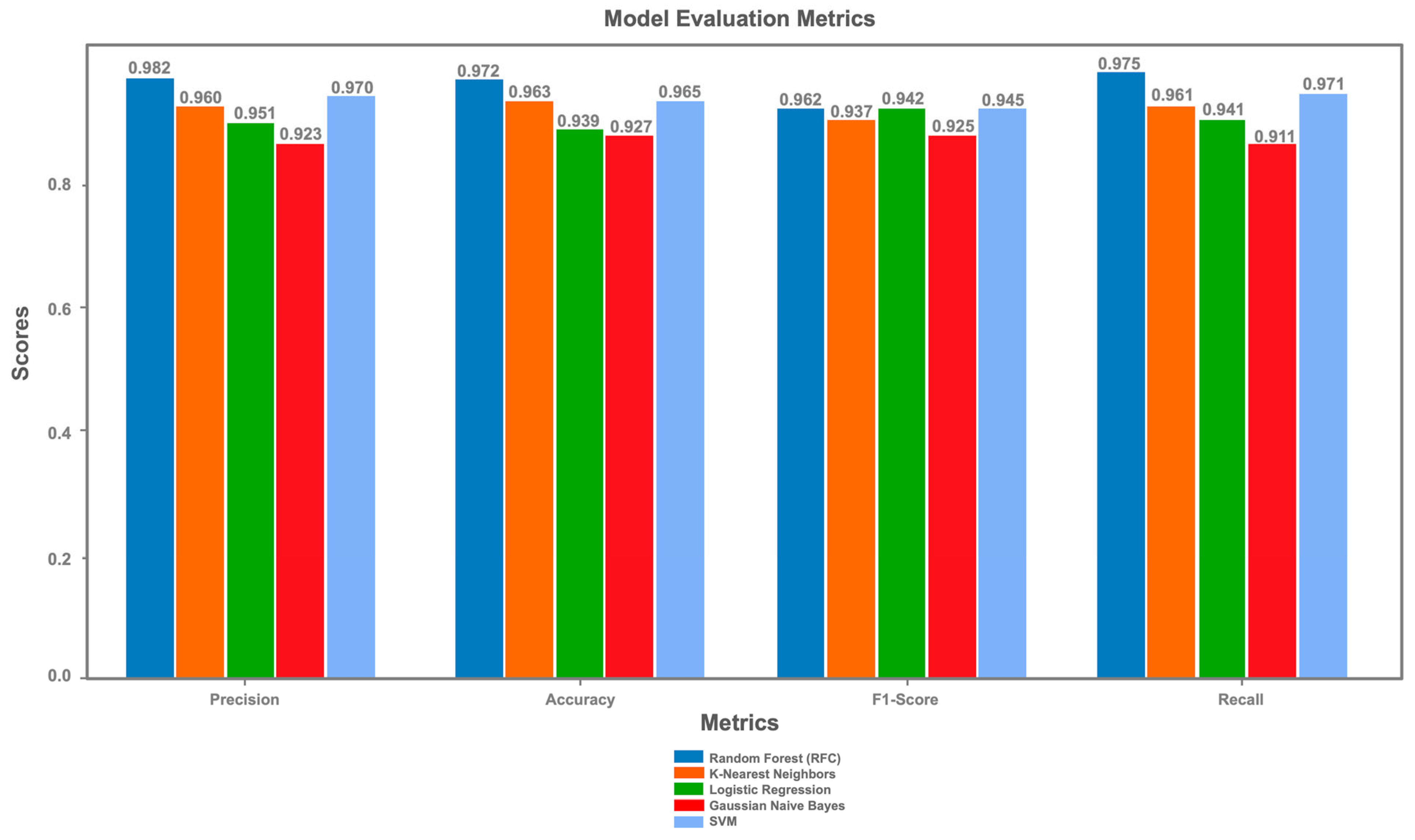
Table 1.
Requirements and Objectives for ML-SOC Design
| Objective/Requirement | Goal | Specific Requirements |
|---|---|---|
| Advanced Threat Detection | Create an ML-SOC capable of accurately detecting threats and identifying anomalies. | Train ML models on both historical and real-time data to identify malicious behavior. |
| Reduction of False Positives | Minimize false alerts to prevent analyst overload. | Develop ML models that can distinguish legitimate activities from malicious behavior with high precision. |
| Rapid Incident Response | Implement automated response mechanisms for quick threat mitigation. | Integrate decision-making algorithms to trigger appropriate response actions. |
| Scalability and Performance | Ensure the architecture can handle large data volumes while maintaining high performance. | Use scalable technologies and infrastructures to adapt to workload increases. |
| Interpretability | Ensure that the ML-SOC’s decisions are explainable for security analysts. | Include mechanisms that provide clear reasoning for triggered alerts. |
Table 2.
Encoded & Clean DATA Sample.
| Day | Hour | Minute | Event Type | Event Name | Source IP | Destination IF | Destination T | Event Severity |
|---|---|---|---|---|---|---|---|---|
| 0.01191466 | 0.00386192 | 1.65453842 | 5 | 1 | 508 | 242 | 13 | 3 |
| 0.01191466 | 0.00386192 | 1.65453842 | 1 | 10 | 1053 | 2677 | 53 | 3 |
| 0.01191466 | 0.00386192 | 1.65453842 | 7 | 3 | 514 | 1696 | 13 | 3 |
| 0.01191466 | 0.00386192 | 1.65453842 | 5 | 1 | 245 | 1138 | 13 | 3 |
| 0.01191466 | 0.00386192 | 1.65453842 | 5 | 1 | 488 | 745 | 13 | 3 |
| 0.01191466 | 0.00386192 | 1.65453842 | 10 | 0 | 617 | 2532 | 1 | 5 |
| 0.01191466 | 0.00386192 | 1.65453842 | 4 | 7 | 376 | 956 | 1 | 3 |
| 0.01191466 | 0.00386192 | 1.65453842 | 4 | 7 | 617 | 2104 | 1 | 3 |
| 0.01191466 | 0.00386192 | 1.65453842 | 4 | 7 | 617 | 2533 | 1 | 3 |
| 0.01191466 | 0.00386192 | 1.65453842 | 5 | 1 | 528 | 1851 | 13 | 3 |
| 0.01191466 | 0.00386192 | 1.65453842 | 7 | 3 | 561 | 2308 | 13 | 3 |
| 0.01191466 | 0.00386192 | 1.65453842 | 3 | 11 | 599 | 951 | 3 | 3 |
| 0.01191466 | 0.00386192 | 1.65453842 | 4 | 7 | 502 | 4 | 1 | 3 |
| 0.01191466 | 0.00386192 | 1.65453842 | 5 | 1 | 238 | 2557 | 13 | 3 |
| 0.01191466 | 0.00386192 | 1.65453842 | 11 | 8 | 490 | 1939 | 13 | 3 |
| 0.01191466 | 0.00386192 | 1.65453842 | 4 | 7 | 616 | 2533 | 1 | 3 |
| 0.01191466 | 0.00386192 | 1.65453842 | 11 | 8 | 569 | 1979 | 13 | 3 |
| 0.01191466 | 0.00386192 | 1.65453842 | 11 | 8 | 603 | 1705 | 13 | 3 |
| 0.01191466 | 0.00386192 | 1.65453842 | 4 | 7 | 616 | 2533 | 1 | 3 |
| 0.01191466 | 0.00386192 | 1.65453842 | 10 | 0 | 502 | 4 | 1 | 5 |
| 0.01191466 | 0.00386192 | 1.65453842 | 4 | 7 | 502 | 2533 | 1 | 3 |
Table 4.
comparative performance of five machine learning models.
| Model | Accuracy | Precision | F1-Score | Recall | True Positive (TP) | True Negative (TN) | False Positive (FP) | False Negative (FN) | True Positive Rate (TPR) | False Positive Rate (FPR) |
|---|---|---|---|---|---|---|---|---|---|---|
| Random Forest (RFC) | 0.972 | 0.982 | 0.978 | 0.975 | 98 | 97 | 3 | 2 | 0.98 | 0.03 |
| K-Nearest Neighbors (KNN) | 0.963 | 0.960 | 0.960 | 0.961 | 95 | 96 | 4 | 5 | 0.95 | 0.04 |
| Logistic Regression | 0.939 | 0.951 | 0.946 | 0.941 | 94 | 95 | 5 | 6 | 0.94 | 0.05 |
| Gaussian Naive Bayes | 0.927 | 0.923 | 0.917 | 0.911 | 90 | 92 | 8 | 10 | 0.90 | 0.08 |
| Support Vector Machine (SVM) | 0.965 | 0.970 | 0.971 | 0.971 | 96 | 96 | 4 | 4 | 0.96 | 0.04 |
Disclaimer/Publisher’s Note: The statements, opinions and data contained in all publications are solely those of the individual author(s) and contributor(s) and not of MDPI and/or the editor(s). MDPI and/or the editor(s) disclaim responsibility for any injury to people or property resulting from any ideas, methods, instructions or products referred to in the content. |
© 2025 by the authors. Licensee MDPI, Basel, Switzerland. This article is an open access article distributed under the terms and conditions of the Creative Commons Attribution (CC BY) license (http://creativecommons.org/licenses/by/4.0/).
Copyright: This open access article is published under a Creative Commons CC BY 4.0 license, which permit the free download, distribution, and reuse, provided that the author and preprint are cited in any reuse.


