Submitted:
25 April 2025
Posted:
25 April 2025
You are already at the latest version
Abstract
Natural disasters, including droughts, exert a profound impact on public health, agriculture, industry, and the environment. The intensification of climate change has exacerbated the frequency and severity of such events. In the context of smart cities, the implementation of advanced prediction methodologies is pivotal for mitigating or even preventing these catastrophic outcomes. Among the most widely employed techniques for time series forecasting are the (S)ARIMA and Holt-Winters exponential smoothing methods, which form the foundation of this study. This research proposes a robust framework for the preprocessing of raw meteorological data, the application of forecasting techniques to monthly observations, and the evaluation of prediction models using standardized performance metrics. The objective is to identify the optimal model for predicting key parameters - such as air temperature, precipitation, and soil moisture - that serve as critical indicators of urban drought conditions. The findings reveal that the SARIMA model demonstrates superior reliability for time series exhibiting a decreasing trend, such as soil moisture, while the Holt-Winters method excels in modeling time series with no trend (e.g., precipitation) and those characterized by strong seasonality, such as air temperature. These insights contribute to the development of more effective urban drought prediction systems and highlight the nuanced applicability of these forecasting methods in addressing climate-related challenges.
Keywords:
(S)ARIMA
; Holt-Winters
; time series forecasting
; urban drought
; smart cities
1. Introduction
Extreme weather events have become more severe in cities due to climate change. As temperatures rise due to global warming, the world is experiencing a shortage of natural resources, such as raw materials, energy sources, and water, especially in populated areas. Climate change is also increasing the natural evaporation of water supplies, leading to dry conditions. This serious problem should be alleviated in part by smart city solutions such as circular economy approaches, involving R9 strategies, which can help with scarce resource conditions [1].
To mitigate the negative effects of such weather conditions and decreased water consumption, it is crucial to monitor and predict climate conditions closely and implement effective water management strategies. Mountains provide freshwater globally and may influence water resource management, climate change adaptation, and water policy. Viviroli examined 11 case study regions to provide a global perspective, highlight research deficiencies, and propose recommendations for research, management, and policy [2].
Forecasting urban drought is a crucial strategy for municipalities and water management organizations. Urban extreme weather can be predicted using statistical forecasting approaches like time series analysis. Analyzing historical meteorological data can reveal city climate trends and patterns. These findings can help predict urban dryness and improve how we respond to extreme climatic events.
Time series models, such as ARIMA and SARIMA, have been widely used in drought prediction by analyzing historical precipitation and temperature data. For instance, Durdu (2010) developed ARIMA and SARIMA models to forecast drought in the Büyük Menderes River basin using the Standardized Precipitation Index (SPI), where the ARIMA model demonstrated superior performance. ARIMA models presume data stationarity and are linear, which can limit them when dealing with complex nonlinear interactions or drought dynamics [3].
In addition to classical statistical methods, ML models are also used for weather analysis. Water resources engineering, planning, and irrigation scheduling need precipitation forecasting. For daily precipitation forecasting, this study compares hybrid wavelet-genetic programming (WGEP) and wavelet-neuro-fuzzy (WNF) models. The first phase employs single genetic programming (GEP) and neuro-fuzzy (NF) models to predict daily precipitation based on past values, although the results are limited. In the next step, hybrid WGEP and WNF models using wavelet coefficients as GEP and NF inputs provide disappointing results despite improved accuracy. In the third step, the best single and hybrid model inputs build new WGEP and WNF models. Kisi, O., & Shiri demonstrate that the novel hybrid WGEP models forecast daily precipitation better than WNF models, which fail to learn the non-linear precipitation process [4].
To investigate drought variability in Denizli, a semi-arid region of Turkey, self-calibrated Palmer Drought Severity Index (sc-PDSI) values were utilized, and projections were conducted for various time horizons: short-term (1 month), mid-term (3 months and 6 months), and long-term (12 months) [5].
Dependable harm Decision-makers need to forecast droughts, largely caused by spatiotemporal precipitation imbalances, to design adaptive measures. Decision-makers need these drought forecasting requirements: The prediction must identify impacted locations and severity, after that severity should be quantified rather than numerically, and at the end it should be completed quickly with minimum information. Ock-Jae Jang developed a drought forecasting method that merges the water balance model with a deep neural network to address these objectives [6].
Some authors have compared classical time series analysis models and ML models for weather forecasting. Drought forecast accuracy is critical for informed land and water resource management as climate change and land use changes increase droughts. This research anticipated drought using the Informer model and compared it to ARIMA, LSTM, and CNN models [7].
The Internet of Things (IoT) is the underlying concept that enables smart cities to forecast weather conditions. IoT devices, such as weather stations, building sensors, and smartphone apps, collect vast amounts of data on atmospheric conditions, temperature, humidity, and wind patterns. Data are then transferred to a central hub for fast processing and analysis. Machine learning algorithms turn collected data into accurate weather predictions, helping individuals, organisations, and governments make sensible decisions. Banara [8] examined smart city IoT weather monitoring systems literature on sensors, microcontrollers, and communication media. The project sought to improve weather monitoring systems by integrating the Internet of Things.
Sreenivasulu [9] demonstrated an efficient IoT-based weather forecasting method for smart cities utilising sensor data. The suggested method exceeded established methods in accuracy and speed. Atta-ur Rahman presented his framework for predicting precipitation in smart cities using fuzzy logic to fuse machine learning methodologies’ predictive accuracy [10]. The effects of soil moisture on seasonal temperature and precipitation prediction scores in Europe have been shown by Van Den Hurk [11].
The analysis of meteorological characteristics was utilized in numerous applications to evaluate gradual trends and forecast weather parameters [12,13,14,15].
Advances in time series forecasting, such as combining statistical methods with machine learning and signal processing, can improve urban drought predictions. These advanced models help managers to understand complex urban climate patterns and trends. Smart cities leverage technology and data analytics to boost productivity, sustainability, and quality of life, revolutionizing our work, lifestyle, and environment. Smart cities need accurate, real-time weather forecasting. Advanced sensors, satellites, and machine learning algorithms can help smart cities predict weather. This enables citizens and local authorities to strategize and prepare for weather-related incidents effectively. The primary advantage of precise weather prediction in smart cities is the ability to anticipate and respond to severe weather occurrences. The occurrence of heatwaves, storms, and floods has increased due to climate change. Precise weather predictions enable local government agencies to strategize, provide emergency aid effectively and, if necessary, evacuate areas with a higher danger risk.
Given that each place on Earth has distinct attributes and traits, the optimal approach to identifying the best model is to start with classical statistical time series models, which will be discussed in this article. This paper will apply, analyses, and compare traditional statistical time series models. In the future, our objective is to use machine learning models to determine which one provides superior predictions based on the available data for specific regions.
Exponential smoothing outperformed complicated statistical methods like autoregressive integrated moving averages (ARIMA) in past time series forecasting contests. There are three types of exponential smoothing algorithms: simple, single, double, and triple. Many approaches use a stochastic process to create observable data, which is influenced by unseen but predictable components, such as local level, trend, and seasonality. The components must be modified when the time series structure changes [16].
Brown and Holt, independently, developed basic exponential smoothing. Winters expanded Holt’s exponential techniques to predict complex time series with seasonality. Their work is recognized by the term Holt-Winters exponential smoothing algorithms. The development of exponential smoothing algorithms relied on heuristics. Thus, model selection and error distribution modelling were unstatistical. Enterprises quickly adopted them for inventory modelling due to their ease of use [17,18,19].
Tihi proposed employing (S)ARIMA time series models to collect, preprocess, and forecast meteorological parameters. The forecasting models were built on data sets of average the air temperature, precipitation, and soil moisture values from January 2014 to December 2018. The paperwork approach was used to manually choose the best (S)ARIMA models. This technique yielded 12 the air temperature, 6 precipitation, and 12 soil moisture time series models with distinct components. The best models for all three time series were chosen using AIC, AICc, BIC, and Ljung-box test p-values [20].
Todorov presented an evaluation-based forecasting model selection process [21]. The strategy was applied to an the air temperature dataset using a SARIMA model. Seasonal model parameters have been automatically chosen. Statistical metrics assessed model performance, including MAE, RMSE, and MAPE.
The study aims to collect and preprocess meteorological data to compare and analyses the efficacy of statistical time series methods and select the optimal model for forecasting drought-related variables. This study employs univariate time series data related to drought, such as the air temperature, precipitation, wind speed, and soil moisture, to build traditional forecasting models, compare them, and visualize their results. Upon comparison, the best predictive model is chosen based on the employed metrics and thereafter utilized for computing drought indexes to categorize the severity of drought and assist decision-makers in formulating drought-related initiatives.
2. Methods
Forecasting Methods
Time series forecasting involves predicting future values based on historical data, and it is a crucial subject in several fields, such as finance, economics, and meteorology. A time series refers to a set of observations or data points, that pertain to a particular variable and are recorded over some time. Time series forecasting uses a range of methods, where the most popular ones are ARIMA and Holt-Winters. These methods can be used in various applications, from forecasting GDP per capita to forecasting primary energy consumption. Also, the efficacy of these data-driven methods in meteorological forecasting applications is very high [22,23,24,25,26].
When making predictions for time series data, it is crucial to assess the characteristics of the data, including trend, seasonality, correlations and any other factors that might impact the accuracy of the model. Model performance should be assessed by using statistical measures, such as Mean Absolute Error (MAE), Root Mean Squared Error (RMSE), or Mean Absolute Percentage Error (MAPE).
(S)ARIMA Methods
Another popular method used in time series forecasting is ARIMA (AutoRegressive Integrated Moving Average) and its seasonal version called SARIMA (Seasonal ARIMA). ARIMA is a statistical model that considers autocorrelation and moving average components of time series data. By analyzing past data and trends, ARIMA can forecast future values with a high level of accuracy [27]. On the other hand, SARIMA is an extension of ARIMA that includes the seasonal component in the model. SARIMA allows for more accurate predictions of seasonal trends and patterns in the data. It can capture the dynamics of a linear system very well [28].
ARIMA forecasting is a commonly used technique for predicting future values of a time series by analyzing its past values. This statistical methodology utilizes sophisticated methods, such as autoregression (AR), moving average (MA) models, and differencing (I), to guarantee the stability of the series. The model integrates autoregressive, moving average, and integrated components to represent the interdependencies and patterns of the series precisely.
Achieving proficiency in ARIMA forecasting requires a thorough comprehension of time series theory and statistical concepts. The Autoregressive component of the model refers to the dependence of current values on prior ones, where the autoregression order (p) determines the number of past values considered. The Moving average component takes into account the impact of prior mistakes on the current result. Moving average order (q) determines the number of previous errors that are considered. Differencing (d) is used to achieve stationarity in a series. This is accomplished by subtracting the prior observation from the current one and eliminating any trend or seasonal influences.
The conventional representation for the non-seasonal ARIMA model is ARIMA (p,d,q), where each parameter is determined by analyzing the autocorrelation function (ACF) and partial autocorrelation function (PACF) of the time series.
The Moving average component indicates the relationship between the current observation and the residual error resulting from applying a moving average model to previous data.
The SARIMA model is used to predict seasonal data, and it incorporates three seasonal components, namely, P, D, and Q, in addition to the three previously described non-seasonal components.
Holt-Winters Exponential Smoothing Method
Brown and Holt [17,18,29] came up with the idea for the basic exponential smoothing approach on their own. In the next step, Winters modified the Holt exponential algorithms, such that they could be used to predict complicated time series that included seasonality [19]. For this reason, the Holt-Winters exponential smoothing techniques were given their name, to recognize their contributions.
Heuristics served as the foundation for the conceptualization of exponential smoothing algorithms in their first form. Considering this, they did not possess a statistical foundation for the selection of models, nor did they have a technique for modeling the distribution of mistakes.
This method is particularly useful for data that exhibit trend and seasonality. Holt-Winters Exponential Smoothing uses weighted averages of past data points to make forecasts for future values. By adjusting the weights for trend and seasonality, the method can provide reliable forecasts, even in the presence of noisy or irregular data. The Holt-Winters method is often preferred for short to medium-term forecasting, due to its simplicity and flexibility in capturing complex patterns in the data.
The Holt-Winters Exponential Smoothing method is a widely used methodology for predicting time series data that exhibit both trends and seasonality. This approach enhances the basic exponential smoothing technique by including three elements: level (α), trend (β), and seasonality (γ). Each component has its parameter, that is used to regulate the impact of the component. These parameters are often established using optimization approaches. The level variable denotes the smoothed value of the time series at the present moment. The trend component of a time series refers to the overall direction and speed of change, whereas seasonality refers to the recurring patterns in the data, such as daily, weekly, or monthly cycles.
The equations for Holt-Winters technique with trend and additive seasonality may be stated as follows:
where:
α (alpha)-level smoothing parameter,
,
.
Holt-Winters, commonly known as triple exponential smoothing may be represented mathematically as:
where:
is the forecast for the m period,
s is the length of seasonality,
is the level of the series,
is the trend component,
is the seasonal component.
Forecasting Metrics
Forecasting metrics are used to evaluate the accuracy and effectiveness of predictive models, particularly those used for time series forecasting. Some of the most used measures are:
The Mean Absolute Error (MAE) is the average of the absolute deviations between the projected and actual values.
Root Mean Squared Error (RMSE) is the square root of the MSE. It uses the same unit as the projected and actual numbers, making it easier to read.
Mean Absolute Percentage Error (MAPE) is the average percentage difference between the anticipated and actual values calculated as the average of the absolute percentage errors.
3. Research
This research is focused on the development of a comprehensive approach for processing and analyzing raw data, with a particular focus on its application to meteorological datasets. The study highlights the integration of statistical methods to improve data quality, enhance predictive accuracy, and extract meaningful insights from complex time series patterns by comparing two traditional methods, such as (S)ARIMA and Holt-Winters. This research aims to serve as a preliminary investigation into the optimal prediction model for parameters that will subsequently be utilised in computing water balance, evapotranspiration, and drought indexes indicative of urban drought severity. The methodology for developing the optimal predictive model starts with data preparation and analysis, followed by the construction of mathematical models, which allows for the systematic examination of time-dependent meteorological factors. The primary objective of selecting the best predictive model is to provide decision-makers with accurate visualized forecasts that may be utilized for strategy development. Principal Component Analysis (PCA) was employed to identify significant relationships among all variables and therefore reduce the dimensionality of the initial dataset. The correlation matrix indicated that the relationships between variables were either moderately negative or weakly positive. Given the absence of significant positive or negative correlations, the decision to utilise the univariate time series data for constructing the prediction models was made. Also, the data were analysed with the Mann-Kendal test to investigate the trend in all four time series.
3.1. Selection of Software
The research results were processed by using the R programming language which is a very famous statistical programming language and environment, used mainly for statistical calculations, data analysis, and visualizations and RStudio (version 2021.09.0 Build 351) which is an Integrated Development Environment (IDE) for R.
3.2. Data Acquisition
The data were obtained from a weather station „WH3” located on a higher river terrace, often called loess or diluvial terrace, near Novi Sad, Serbia from January 2014 until December 2020. The higher river terrace is minimally dissected, and its surfaces are suitable for the unhindered expansion of the settlement. Water supply is easy, most of the areas are safe from floods, and the conditions for agriculture production and traffic flow are optimal. It covers about 38% of the area of Vojvodina.
This weather station, shown in the Figure 1, consists of various sensors, which can be categorized into seven groups. The first group represents six sensors that measure only soil moisture (SM1, SM2, SM3, SM4, SM5, SM6). These sensors are divided into three subgroups depending on the soil depth at which they are located. In the first subgroup, closer to the surface, there are sensors SM1 and SM2, one from the left and one from the right side. At the next depth there are sensors SM3 and SM4 and at the greatest depth there are sensors SM5 and SM6. The other sensor group categories include a humidity sensor (AH1), wind speed (WS1), wind direction (WD1), the air temperature (AT1), precipitation (PP1), and battery power state (BT1). Since there are 12 sensor groups that record measurements hourly, there are 288 records in total per 24 hours across all sensor groups. For this research, only the measurements from the the air temperature, precipitation, soil moisture and wind speed sensors were taken. The air temperature was measured in degrees Celsius, precipitation in millimeters, wind speed in m/s and soil moisture in percentage of volume. The data set consists of four attributes: time, device, ID value, and value. Descriptions of all four attributes are given in Table 1 [30].
3.3. Data Preparation
After the hourly measurements have been retrieved from the online portal in Excel format, they are converted and then stored in a data frame. A data frame is a basic data structure used to store and organize tabular data. The first step is to prepare the data. The preparation process includes filtering, aggregating, sorting, and, finally, saving the data as a time series. The the air temperature, wind speed, precipitation and soil moisture time series are aggregated to obtain the average daily values. After being aggregated, the data are arranged in ascending order according to the observed date and then converted into time series entities. The dataset of 2553 observations is ultimately partitioned based on time into two subsets by using a straightforward and widely used time series splitting method called Holdout or Fixed split. 80% of the original dataset was used for training set and the rest was used for validation set for model verification.
3.4. Data Modelling
After the data were prepared, partitioned and analyzed for dimensionality reduction and trend, the next step was the modeling phase. Four predictive models of (S)ARIMA and Holt-Winters were built, each for every time series using functions from forecast package version 8.24.0. Optimal (S)ARIMA parameters can be very challenging to select so the selection process of the best appropriate values for seasonal ARIMA parameters was performed automatically [31].
4. Results
4.1. Graphical Representation
Before building models, the data needss to be visualized in the form of a line graph with points [30]. All four of the time series, one for every parameter, are presented in Figure 2, Figure 3, Figure 4 and Figure 5. Figure 6 shows all the parameters displayed within one graph.
Figure 2 shows the average daily temperatures in the period from January 2014 to December 2020. There is a very strong regular annual cycle, and peaks occur around mid-year and the end of each year. This indicates that the temperature changes with the seasons. Since there are no obvious upward and downward shifts across the years, temperature levels remained relatively stable over the period, which the Mann-Kendall test confirmed. The p-value was 0.6569, which clearly showed that there was no trend since the null hypothesis could be rejected. There are some outliers, such as the lowest temperature in January 2017 and the hottest in August 2017.
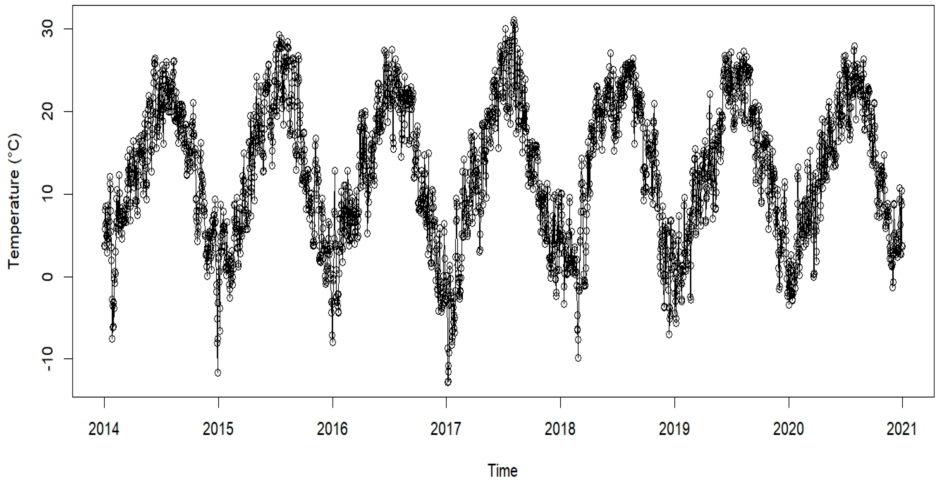
Figure 2.
Daily average temperatures (℃) from 2014 to 2021.
Figure 3 displays the total amount of precipitation. The graph shows that most days have little or no precipitation and rainfull occurs in short intense bursts. Spikes vary in height, with some days showing precipitation over 50 mm. There is no obvious seasonality pattern and long-term trend which the Mann-Kendall test confirmed (null hypothesis was rejected due to p value of 0.1528). The highest amount of precipitation was in May 2014.
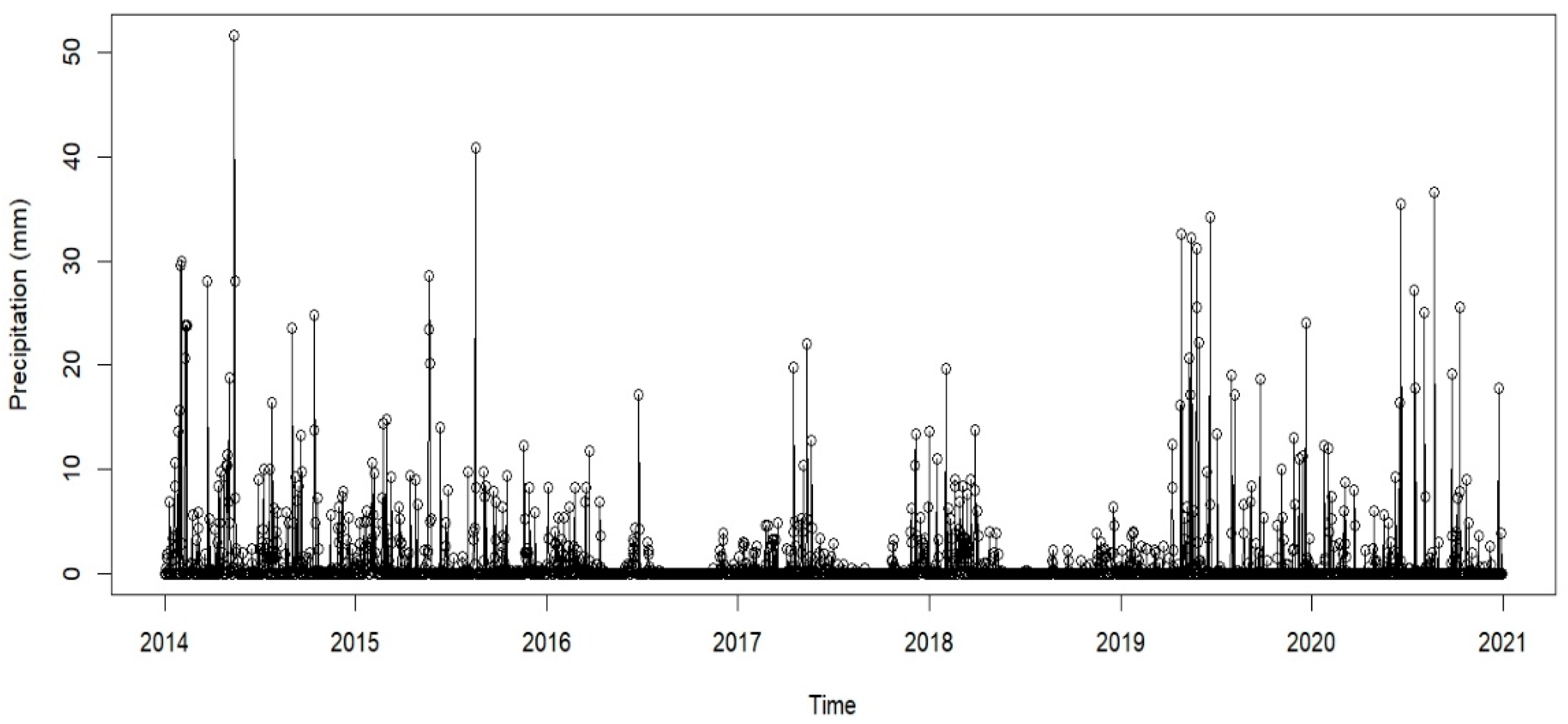
Figure 3.
Daily total precipitation (mm) from 2014 to 2021.
Figure 4 shows the average soil moisture over time. It can be concluded from the graph that the soil moisture levels vary periodically, presumably due to seasonal precipitation patterns. Higher values correspond to wetter conditions (rainy season), while lower values indicate dry conditions. The data shows a gradual decline in soil moisture from 2014 to 2021, which could indicate increasing dryness, reduced precipitation, or changes in soil characteristics. Some periods, like 2019 and 2020, show particularly low moisture values, potentially indicating drought conditions. Sharp increases in soil moisture suggest rainfall events or irrigation. Significant declines indicate drying periods due to high temperatures, evaporation, or reduced rainfall. A decreasing trend was detected with the Mann-Kendall test in this time series. (p-value was 3.284048567153697e-05).
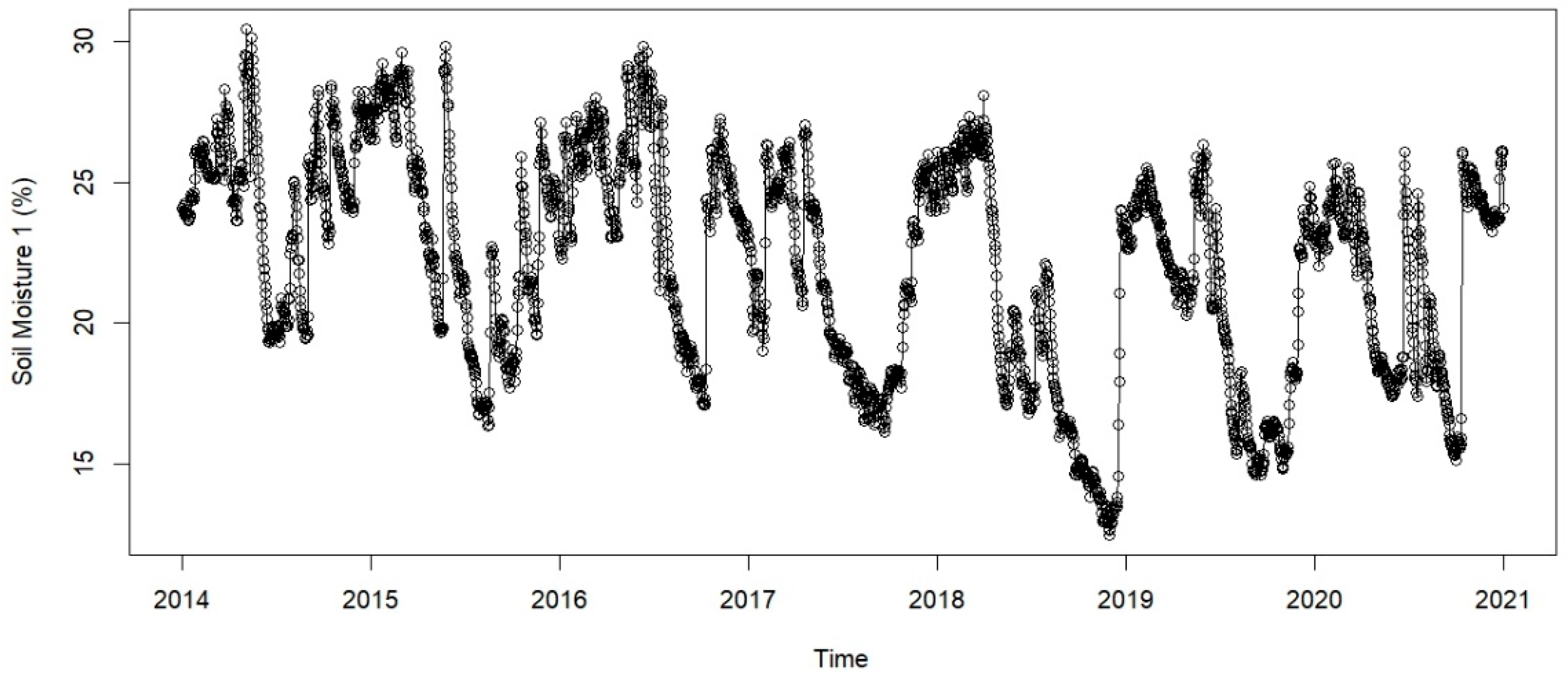
Figure 4.
Daily average soil moisture from 2014 to 2021.
Figure 5 shows the average daily wind speed. It is noticeable that wind speed has significant peaks at approximately regular annual periods, indicating a seasonal pattern. Certain extreme peaks are prominent, perhaps indicative of severe weather phenomena such as winter storms. The dataset exhibits high variability, with frequent spikes in wind speed, indicating occasional strong winds or storm events. Some peaks reach above 2.5 m/s, while the majority of the values stay below 1 m/s. While there is no clear upward or downward trend (p-value on the Mann-Kendall test was 0.7044 ) in wind speed over the years, the fluctuations appear consistent.
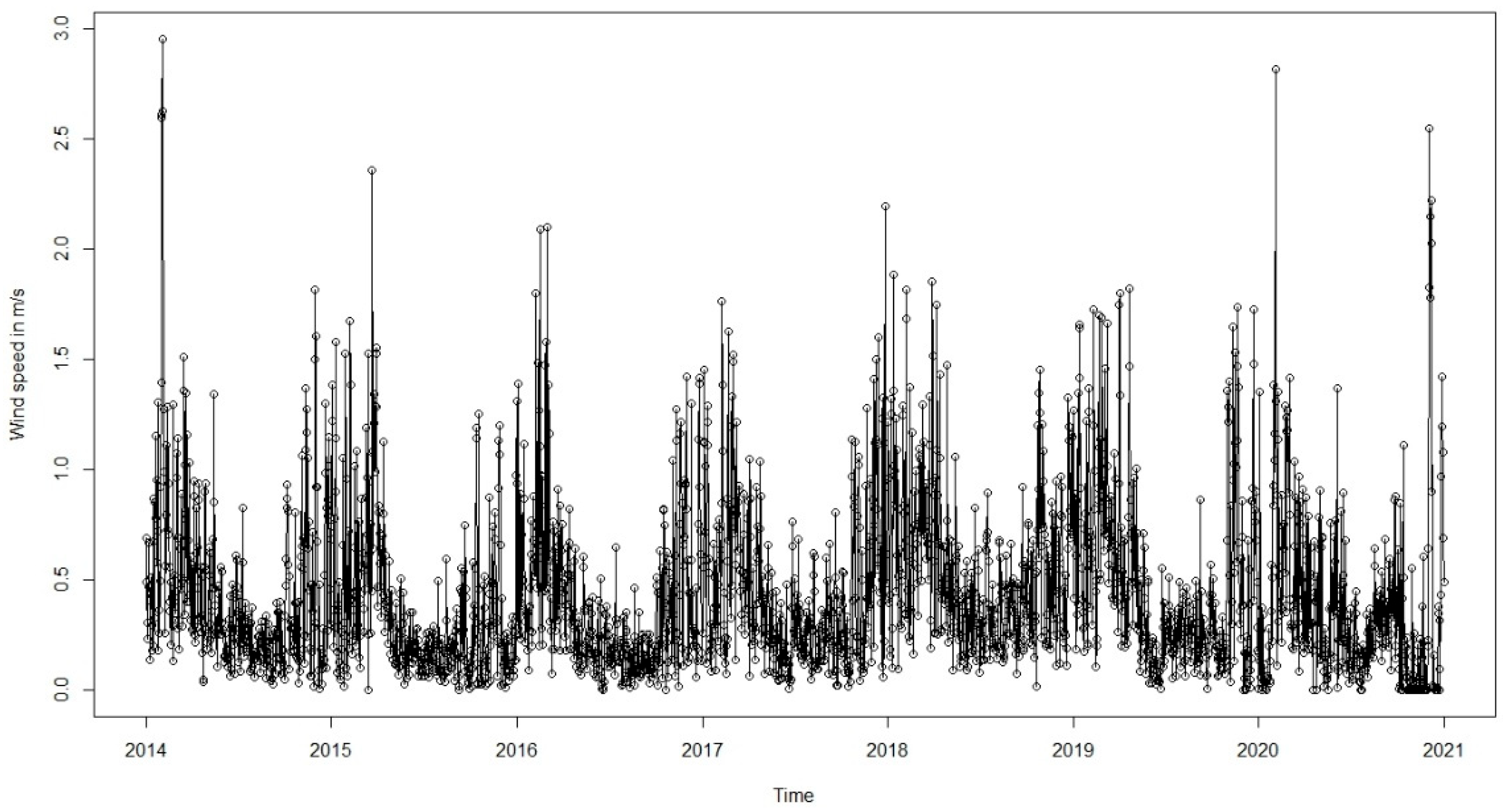
Figure 5.
Daily average wind speed from 2014 to 2021.
All the parameters within one graph are displayed in Figure 6. It can be noticed that seasonal trends are visible in temperature and soil moisture. Increased soil moisture coincides with rainfall surges, and dry seasons likely result in a decrease in soil moisture, with temperature inversely affecting it. Wind speed remains relatively stable compared to other variables.
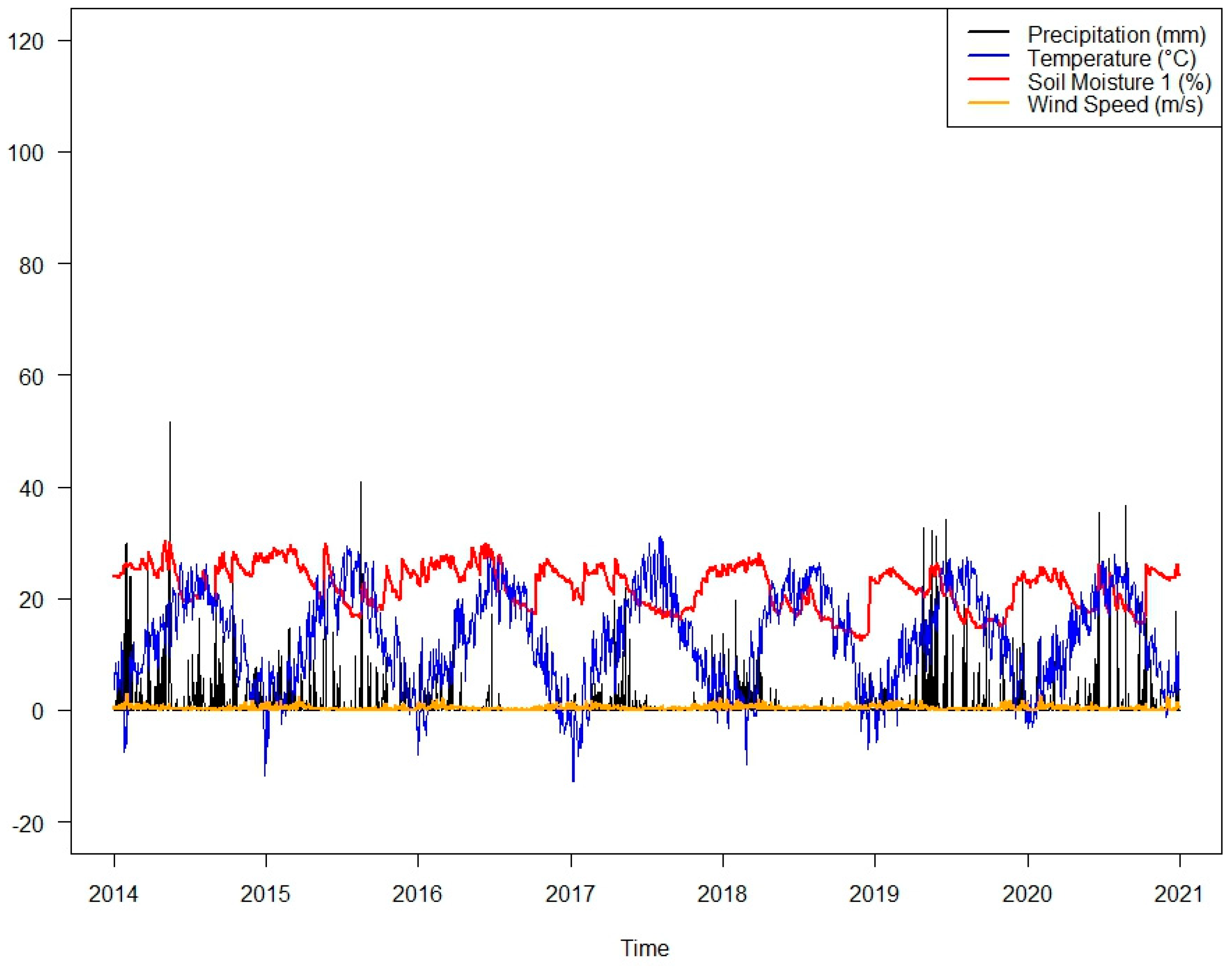
Figure 6.
All the daily averaged parameters displayed in one graph.
4.2. Results of the ARIMA Method
Given the difficulty and time consumption associated with determining the appropriate model for a time series, the ideal ARIMA parameters were determined automatically. It was found that the best selected predictive model for the air temperature daily time series was SARIMA (3,0,0)(0,1,0)[365], for precipitation time series was the ordinary ARIMA (5,1,3), for soil moisture time series was ARIMA (3,0,0) and for wind speed was ARIMA (3,1,2).
The models and their criteria values (AIC, AICc, BIC) for all four time series, are shown in Table 2.
The forecasted data, obtained from the best-selected SARIMA model for the the air temperature time series, along with historical and validation data, are shown in Figure 7. The green line represents historical data, while the blue line represents validation data. The red line displays the forecasted values for 24 months ahead. It can be concluded that the forecasted values are pretty accurate compared to the actual validation data, and, therefore, the model is very fit. The value of RMSE of the model was 2.748819, which is quite low, indicating good model performance.
Figure 8 shows the forecasted, historical, and validation data obtained from the selected ARIMA model for the precipitation time series. In order to avoid zero values in precipitation we had to build a model on a log-transformed data. The forecasted values appear centered around zero, indicating that the ARIMA model may struggle with capturing seasonal trends or non-stationarity in the data. The predicted values fall significantly below observed values, suggesting that ARIMA might not fully capture extreme variations. The confidence intervals remain narrow but less compared with untransformed data, likely due to the log transformation stabilizing variance. By analyzing the metrics of the model, it is noticeable that the value of RMSE (Root Mean Squared Error) was 0.545284, which is not considered very high. The higher RMSE indicates larger errors and potentially poorer model performance.
Figure 9 displays the forecasts from the selected ARIMA model for soil moisture daily time series. The forecast captures the general seasonal trend of soil moisture but demonstrates growing uncertainty over time (as seen in the widening confidence intervals). The central forecast (red line) follows a cyclical trend similar to historical patterns, indicating that the ARIMA model has captured some seasonality. The wide confidence intervals (highlighted in red) suggest considerable uncertainty in long-term forecasts, which is common in ARIMA models for time series with strong fluctuations. The forecasts initially aligns with the validation data but diverges over time, suggesting possible constraints in capturing long-term trends. Also, not very high RMSE (RMSE=0.4791969) indicates minor errors. However, the model can be improved by fine-tuning the parameters, in order to increase the performance.
Figure 10 displays the forecasts from the selected ARIMA model for wind speed daily time series. The graph shows that the ARIMA model effectively captures seasonality in wind speed. Short-term forecasts are plausible, as the model closely adheres to the trends observed in the validation data. The increasing confidence interval suggests higher uncertainty in long-term forecasts. Since ARIMA is a linear model, it may struggle with capturing non-linear connections or rapid fluctuations in wind speeed. Also, not very high RMSE (RMSE=0.1516107) indicates minor errors. However, the model can be improved by fine-tuning the parameters, in order to increase the performance
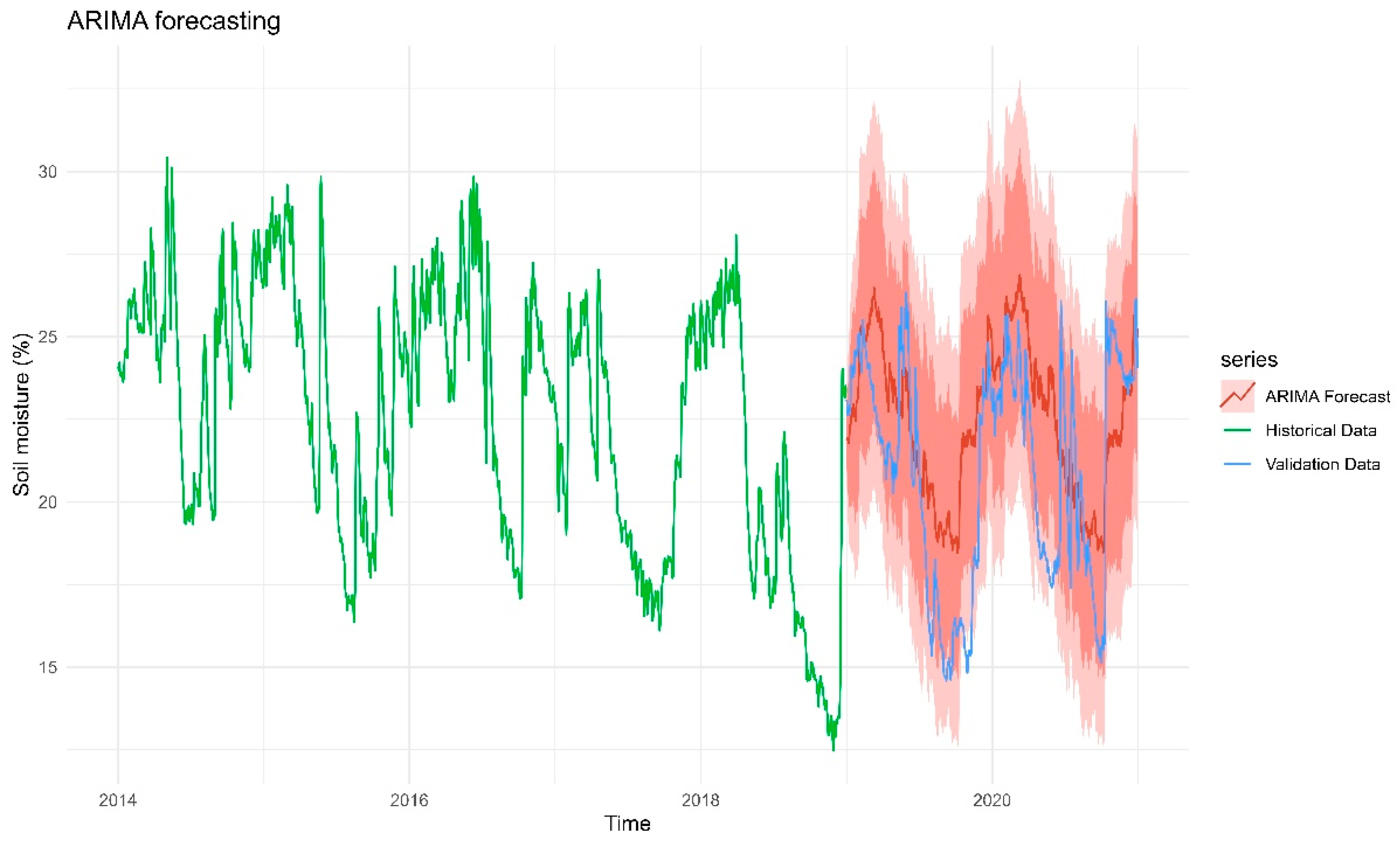
Figure 9.
Forecasts from the ARIMA model for the soil moisture time series.
4.3. Results of the Holt-Winters Method
Another technique used for building predictive models was the Holt-Winter method. Table 3 shows the information criteria values (AIC, AICc, BIC) of all four Holt-Winters models.
The forecasts from the Holt-Winters additive method for the time series Temperature are displayed in Figure 11. The original data are shown by the red line in the graph, while the modeled data are shown by the green line. The blue line represents the validation data, which are used to verify the performance of the selected model. The model captures the regular seasonal up-and-down patterns (summers and winters) quite well. The forecast (green) closely follows the validation data (blue), especially in the first half of the forecast window. Toward the end of the forecast period, there’s some deviation—the forecast overshoots or undershoots the validation data slightly but this is expected, as forecasting uncertainty increases further into the future. Also, according to the value of RMSE, which is moderate (RMSE=2.934332), it can be concluded that the forecasted values deviate from the actual (validation) temperature by about 2.93 ℃. Since temperature values range from -10°C to 30°C, a ~3°C error is moderate but acceptable, and the model could be improved by fine-tuning the Holt-Winters parameters.
Figure 12 shows the forecasts from the Holt-Winters additive method for the precipitation time series. Green line in the graph shows the forecasted values of one year for log-transformed precipitation time series. Forecasted values are noticeably smoother and lower amplitude compared to the validation data. They include some negative values which is unrealistic for precipitation. Blue line represents validation data which is actual observed precipitation post-training period. It displays much sharper and more frequent peaks suggesting high short-term variability. It can be concluded that Holt-Winters struggles to capture the peak intensity or frequency of rainfall in the validation period. Negative forecast values which are unrealistic indicates limitation of the additive Holt-Winters model. The precipitation dataset seems to have random or weakly seasonal behaviour which Holt-Winters struggles to capture so as a result, the model forecasts a muted and inaccurate signal. Since RMSE is modest (RMSE=0.7304) and penalizes large errors more heavily, it can be concluded that this model has poor performance and needs to be improved.
Figure 13 shows the forecasts from the Holt-Winters additive method for the log-transformed daily soil moisture time series, which covers historical data from 2014 to the end of 2018. The historical data, which are represented by the red line, show a clear seasonal pattern with soil moisture levels rising and falling cyclically. There is a noticeable downward drift toward the end of the historical period, indicating a possible long-term drying trend. The model captures general trend and seasonality pretty well, following similar cycles. The model is trained on log-transformed data, which helped stabilise variance. However, it seems to slightly underestimate peaks and troughs — possibly due to smoothing from the additive model. According to the RMSE value (RMSE=0.03287), model has small average squared errors.There is a good amount of overlap with the actual validation data, suggesting the model is well-calibrated. The forecast may miss extreme values, but that is common for this method.
Figure 14 shows forecasts from the Holt-Winters additive method for the log-transformed daily wind speed time series. The historical data (red line) shows a clear seasonal pattern – possibly annual cycles with peaks and troughs repeating. The green forecast line aligns pretty well with the general trends and seasonal variations of the blue validation data. However, there exist certain discrepancies—specifically the underestimate of severe peaks or abrupt declines.This is common in Holt-Winters models when the data exhibits significant volatility. Also RMSE value of the model (RMSE=0.2196489) is suggesting that the model’s forecasts are fairly close to the actual values. The conclusion is that the model effectively captures the cyclical patterns in wind speed data and yields a plausible forecast. The model’s smoothing characteristics result in the omission of certain extreme deviations, which is anticipated.
5. Discussion
After the process of building the models is done, the models’ produced results must be compared. The comparison was conducted using three accuracy measures: Mean Absolute Error (MAE), Root Mean Square Error (RMSE), and Mean Absolute Percentage Error (MAPE). The metrics results of both models for all three of the time series are shown in Table 4, Table 5 and Table 6, respectively.
Table 4 demonstrates that the ARIMA technique consistently outperforms the Holt-Winters model across all three error metrics. Although both performance indicators, RMSE and MAPE, describe the dispersion of the observations around the mean, they are not on the same scale, therefore equivalent results cannot be predicted. The root mean squared error (RMSE) often takes precedence over other statistical measures and serves as a reliable indication of model quality. However, when comparing multiple models, it is also important to include not only the RMSE values but also the values of some other performance indicators, like mean absolute error (MAE) or mean absolute percentage error (MAPE). The Holt-Winters method may not be adequately capturing the seasonality compared to ARIMA model. According to the lower values for all three error metrics, it can be concluded that the ARIMA model is the most suitable model for fitting the the air temperature data.
Table 5 shows the accuracy performance indicators of both models for the precipitation time series. The RMSE and MAE values of the HW model are higher compared to the ARIMA model, which indicates that the ARIMA model performs better when data are log-transformed. The Mean absolute percentage error (MAPE) is calculated as the average of the (actual-predicted)/abs(actual), and the lower the value is, the better the model is. One of its limitations is that this evaluation metric is inefficient when the data contain very extreme values. Since some of the actual average values in the time series are zero, or close to zero due to no or little precipitation that particular month, the function for calculating this measure returned an infinity value. To overcome this issue, MAPE should be replaced with an alternative regression metric like symmetric mean absolute percentage error (SMAPE) or a weighted MAPE [32,33]. For this time series, ARIMA clearly outperfoms Holt-Winters based on MAE and RMSE.
The accuracy results of both models for the soil moisture time series are shown in Table 6. All three accuracy performance indicators are lower for the Holt-Winters model compared to the ARIMA model. This suggests that Holt-Winters performs significantly better, making more accurate predictions compared to ARIMA model. RMSE is particularly higher than Holt-Winters, indicating that ARIMA may be overfitting/underfitting or it may have a higher variance. Therefore, the conclusion is that the Holt-Winters is the superior model in the comparison to ARIMA and it may be capturing the underlying trend/seasonality iif the data more effectively than ARIMA.
The results of both models’ measures for the wind speed time series are shown in Table 7. MAE value is lower for ARIMA which suggests that the absolute difference between the predicted and actual values is smaller, meaning that this model provides more consistent forecasts. As for RMSE, it is also lower for ARIMA model, indicating that this model is less prone to significant deviations or extreme forecast mistakes. RMSE imposes a greater penalty on higher mistakes compared to MAE, hence reinforcing the robustness of ARIMA. MAPE vlaues for both models are infinite due to possible zero or near-zero actual values. ARIMA’s ability to capture temporal dynamics and autoregressive behaviour outperforms the Holt-Winters model for the wind speed time series.
6. Conclusion
Time series forecasting uses statistical approaches to predict future values of a changing dataset based on previous observations. Economics, finance, and meteorology use it to make informed decisions. ARIMA and its seasonal version called SARIMA are popular time series analysis methods. ARIMA uses autocorrelation and moving average components, while SARIMA uses seasonal components for better predictions. The Holt-Winters Exponential Smoothing approach is frequently used for short to medium-term forecasting due to its simplicity and versatility in capturing complicated data patterns.
This study demonstrated the methodology for selecting the optimal forecasting model using certain evaluation performance indicators, such as RMSE, MAPE, and MAE. Four methods were applied to the temperature, precipitation, soil moisture and wind peed daily datasets. Three (S)ARIMA methods and one exponential smoothing method were used. Based on accuracy measures for each dataset, the Holt-Winters model with additive seasonality forecasted soil moisture daily average time series best, while ARIMA was best for precipitation and wind speed time series. SARIMA was ideal for forecasting temperature time series.
To enhance the accuracy of forecasting models, future research should explore the application of hybrid approaches, such as combining ARIMA with Artificial Neural Networks (ANN) [34], which should perform better than just using one model, or enhancing the precision of the existing prediction models by the acquisition of more data and fine-tuning the models’ parameters. This integration leverages the strengths of both models, potentially outperforming the use of a single model alone. For instance, a study developed a hybrid forecasting framework that integrates two different models to improve prediction capability [35]. Additionally, refining existing prediction models through the acquisition of more comprehensive data and fine-tuning model parameters is crucial. A systematic review of hybrid forecasting methods emphasises the importance of parameter optimisation for enhancing model performance [36]. Furthermore, studies have shown that developing hybrid models that combine different forecasting techniques improves accuracy. For instance, a study suggested a mixed model using Empirical Mode Decomposition (EMD) and ARIMA to predict long-term streamflow, which worked better than either model alone [37]. In summary, adopting hybrid modeling approaches and focusing on parameter optimization is a promising strategy for improving the precision of precipitation forecasting models.
The selection and development of algorithms play a fundamental role in all the research involving the application of mathematical models to energy systems and scientific investigations. Effective algorithms enable accurate simulations, optimize resource management, and enhance predictive capabilities; ultimately, they improve efficiency and decision-making in complex energy networks. By refining computation methods, researchers can better analyze system dynamics, forecast demand, and develop sustainable solutions tailored to real-world challenges [38,39,40,41,42].
References
- Alivojvodić, V.; Kokalj, F. Drivers and barriers for the adoption of circular economy principles towards efficient resource utilisation. Sustainability 2024, 16(3), 1317; ISSN 2071-1050. COBISS.SI-ID 183683331. [CrossRef]
- Viviroli, D.; Archer, D.R.; Buytaert, W.; Fowler, H.J.; Greenwood, G.B.; Hamlet, A.F.; Huang, Y.; Koboltschnig, G.; Litaor, M.I.; López-Moreno, J.I.; Lorentz, S.; Schädler, B.; Schreier, H.; Schwaiger, K.; Vuille, M.; Woods, R. Climate change and mountain water resources: Overview and recommendations for research, management, and policy. Hydrology and Earth System Sciences 2011, 15(2), 471–504. [Google Scholar] [CrossRef]
- Durdu, Ö.F. Application of linear stochastic models for drought forecasting in the Büyük Menderes river basin, western Turkey. Stochastic Environmental Research and Risk Assessment 2010, 24(8), 1145–1162. [Google Scholar] [CrossRef]
- Kisi, O.; Shiri, J. Precipitation forecasting using wavelet-genetic programming and wavelet-neuro-fuzzy conjunction models. Water Resources Management 2011, 25(13), 3135–3152. [Google Scholar] [CrossRef]
- Akyüz, E.; Şen, Z. Drought Forecasting Using Integrated Variational Mode Decomposition and XGBoost Algorithm: A Case Study of Denizli, Turkey. Water 2023, 15(19), 3413. [Google Scholar]
- Jang, O.-J.; Moon, H.-T.; Moon, Y.-I. Drought Forecasting for Decision Makers Using Water Balance Analysis and Deep Neural Network. Water 2022, 14(12), 1922. [Google Scholar] [CrossRef]
- Shang, Y.; Li, X.; Zhang, T. Enhancing Drought Forecast Accuracy Through Informer Model: A Case Study in the Songliao River Basin. Land 2023, 14(1), 126. [Google Scholar]
- Banara, S.; Singh, T.; Chauhan, A. IoT Based Weather Monitoring System for Smart Cities: A Comprehensive Review. 2022 International Conference for Advancement in Technology (ICONAT); 2022; pp. 1–6. [Google Scholar] [CrossRef]
- Bolla, S.; Anandan, R.; Thanappan, S. Weather Forecasting Method from Sensor Transmitted Data for Smart Cities Using IoT. Scientific Programming 2022, 2022, 1–9. [Google Scholar] [CrossRef]
- Rahman, A.; Abbas, S.; Gollapalli, M.; Ahmed, R.; Aftab, S.; Ahmad, M.; Khan, M.A.; Mosavi, A. Rainfall Prediction System Using Machine Learning Fusion for Smart Cities. Sensors 2022, 22(9), 3504. [Google Scholar] [CrossRef]
- Van Den Hurk, B.; Doblas-Reyes, F.; Balsamo, G.; Koster, R.D.; Seneviratne, S.I.; Camargo, H. Soil moisture effects on seasonal temperature and precipitation forecast scores in Europe. Climate Dynamics 2012, 38(1–2), 349–362. [Google Scholar] [CrossRef]
- Do, H.X.; Westra, S.; Leonard, M. A global-scale investigation of trends in annual maximum streamflow. Journal of Hydrology 2017, 552, 28–43. [Google Scholar] [CrossRef]
- Gocic, M.; Trajkovic, S. Analysis of changes in meteorological variables using Mann-Kendall and Sen’s slope estimator statistical tests in Serbia. Global and Planetary Change 2013, 100, 172–182. [Google Scholar] [CrossRef]
- Krtolica, I.; Todorov, M.; Prohaska, S.; Stojković, M. Annual and Low-Flow Trends in Serbia. Journal of Hydrologic Engineering 2024, 29(3), 05024008. [Google Scholar] [CrossRef]
- Stojković, M.; Prohaska, S.; Plavšić, J. Stochastic structure of annual discharges of large European rivers. Journal of Hydrology and Hydromechanics 2015, 63(1), 63–70. [Google Scholar] [CrossRef]
- Huang, S.h.; Dong, Y. An active learning system for mining time-changing data streams. Intelligent Data Analysis 2007, 11(4), 401–419. [Google Scholar] [CrossRef]
- Brown, R.G.; Davies, O.L. Statistical Forecasting for Inventory Control. Journal of the Royal Statistical Society. Series A (General) 1960, 123(3), 348–349. [Google Scholar] [CrossRef]
- Holt, C.C. Forecasting seasonals and trends by exponentially weighted moving averages. ONR Memorandum, Vol. 52, Carnegie Institute of Technology, Pittsburgh. Available from the Engineering Library, University of Texas, Austin. 1957. [Google Scholar]
- Winters, P.R. Forecasting Sales by Exponentially Weighted Moving Averages. Management Science 1960, 6(3), 324–342. [Google Scholar] [CrossRef]
- Tihi, N.; Popov, S. Selection of the Best ARIMA Models for Urban Drought Prediction. Fresenius Environmental Bulletin (FEB) 2023, 32(06), 2564–2572. [Google Scholar]
- Todorov, M.; Tihi, N.; Popov, S.; Stamatovic, B. Time series models for weather forecasting in smart cities, International Scientific Conference ”ALFATECH – Smart Cities and modern technologies”, Belgrade, Serbia. 2024. [Google Scholar]
- Dritsaki, M.; Dritsaki, C. Comparison of the Holt-Winters Exponential Smoothing Method with ARIMA Models: Forecasting of GDP per Capita in Five Balkan Countries Members of European Union (EU) Post COVID. Modern Economy, 2021; 12, 12, 1972–1998. [Google Scholar] [CrossRef]
- Rahman, A.; Ahmar, A.S. Forecasting of Primary Energy Consumption Data in the United States: a comparison between ARIMA and Holt-Winters Models. AIP Conference Proceedings 2017, 1885(01), 020163. [Google Scholar] [CrossRef]
- Lidiema, C. Modeling and Forecasting Inflation Rate in Kenya Using SARIMA and Holt-Winters Triple Exponential Smoothing. American Journal of Theoretical and Applied Statistics 2017, 6(3), 161. [Google Scholar] [CrossRef]
- Murat, M.; Malinowska, I.; Gos, M.; Krzyszczak, J. Forecasting daily meteorological time series using ARIMA and regression models. International Agrophysics 2018, 32(2), 253–264. [Google Scholar] [CrossRef]
- Tan, K.C. Trends of rainfall regime in Peninsular Malaysia during northeast and southwest monsoons. Journal of Physics: Conference Series 2018, 995, 012122. [Google Scholar] [CrossRef]
- Wan, Y.; Chen, Y.; Yan, C.; Zhang, B. Similarity-based sales forecasting using improved ConvLSTM and prophet. Intelligent Data Analysis 2021, 25(02), 383–396. [Google Scholar] [CrossRef]
- Wang, D.; Wang Ch Xiao, J.; Xiao, Z.; Chen, W.; Havyarimana, V. Bayesian optimization of support vector machine for regression prediction of short-term traffic flow. Intelligent Data Analysis 2019, 23(02), 481–497. [Google Scholar] [CrossRef]
- Syntetos, A.A.; Boylan, J.E.; Disney, S.M. Forecasting for inventory planning: A 50-year review. Journal of the Operational Research Society 2009, 60 (Suppl. 1), S149–S160. [Google Scholar] [CrossRef]
- Tihi, N.; Popov, S.; Bondžić, J.; Dujović, M. Visualization of Big Data as Urban Drought Monitoring Support in Smart Cities. Fresenius Environmental Bulletin 2021, 30(01), 716–722. [Google Scholar]
- Tihi, N.; Popov, S.; Kavalić, M. A Comparison of Seasonal Arima and Holt-Winters Exponential Smoothing Models for Urban Drought Prediction. In B. Savić (Ed.), Book of proceedings. Vol 3 / International Multidisciplinary Conference "Challenges of Contemporary Higher Education" - CCHE 2024, Kopaonik January 29th - February 3rd 2024 (pp. [404-411]). Belgrade: Conference of Academies for Applied Studies in Serbia (CAASS), University Business Academy in Novi Sad, Faculty of Contemporary Arts. ISBN-978-86-82744-04-7; ISBN 978-86-82744-00-9 (series). COBISS.SR-ID 139350281. Savić, B., Ed.; 2024. [Google Scholar]
- Goodwin, P.; Lawton, R. On the Asymmetry of the Symmetric MAPE. International Journal of Forecasting 1999, 15, 405–408. [Google Scholar] [CrossRef]
- Kolassa, S.; Schütz, W. Advantages of the MAD/Mean Ratio over the MAPE. Foresight: The International Journal of Applied Forecasting, International Institute of Forecasters 2007, 6, 40–43, Spring. [Google Scholar]
- Büyükşahin, Ü.Ç.; Ertekin, Ş. Improving forecasting accuracy of time series data using a new ARIMA-ANN hybrid method and empirical mode decomposition. Neurocomputing 2019, 361, 151–163. [Google Scholar] [CrossRef]
- Zhu, Y.; Li, X. A Hybrid Forecasting Framework Integrating Two Different Models to Improve Prediction Capability. Applied Sciences 2023, 14(16), 7122. Available online: https://www.mdpi.com/2076-3417/14/16/7122.
- Khan, M.T.; Rehman, M.U. A Systematic Review on Hybrid Forecasting Methods and the Importance of Parameter Optimization. Electronics 2023, 12(9), 2019. Available online: https://www.mdpi.com/2079-9292/12/9/2019.
- Liu, H.; He, W. Long-Term Streamflow Forecasting Using a Hybrid Model Based on Empirical Mode Decomposition and ARIMA. Water 2018, 10(7), 853. Available online: https://www.mdpi.com/2073-4441/10/7/853.
- Popović, S.; Đukić, D.; Popović, D.S.; Kopanja, L. Preliminary Research on the Application of Neural Networks to the Combustion Control of Boilers with Automatic Firing. In Proceedings of the 8 th Virtual International Conference on Science Technology and Management in Energy; 2022; pp. 299–303, ISBN 978-86-82602-01-9. COBISS.SR-ID 119331337. [Google Scholar]
- Popović, S.; Viduka, D.; Bašić, A.; Dimić, V.; Djukic, D.; Nikolić, V.; Stokić, A. Optimization of Artificial Intelligence Algorithm Selection: PIPRECIA-S Model and Multi-Criteria Analysis. Electronics 2025, 14(3), 562. [Google Scholar] [CrossRef]
- Popović, S.; Denić, N.; Stojanović, J.; Đukić, D.; Popović, S.Đ. Innovations in Risk Management-Integration of Neural Networks in Boilers with Automatic Firing. PaKSoM 2024, 2024, 249. [Google Scholar]
- Popovic, S.; Djukic, D.; Popovic, S.D.; Gligorijevic, M. Neural networks in pellet combustion control - an overview of the group’s research work in 2022/2023. Procedings of 9th Virtual International Conference on Science, Technology and Management in Energy, Belgrade, Serbia; 2023; pp. 249–254, ISBN 978-86-82602-03-3. COBISS.SR-ID 139266057. [Google Scholar]
- Popovic, S.D. Multi-objective mathematical optimization in the smart city supply planning problem. Proceeding of International Scientific and Professional Conference “ALFATECH“Smart Cities and modern technologies, Belgrade, Serbia, 15 March 2024; 2024; p. 20, ISBN 978-86-6461-074-2. UDK: 711.45:004.7005.591.1:004.7, COBISS.SR-ID 148861705, DOI: 10.5281/zenodo.12615013. [Google Scholar]
Figure 1.
The footage of the weather station WH3.
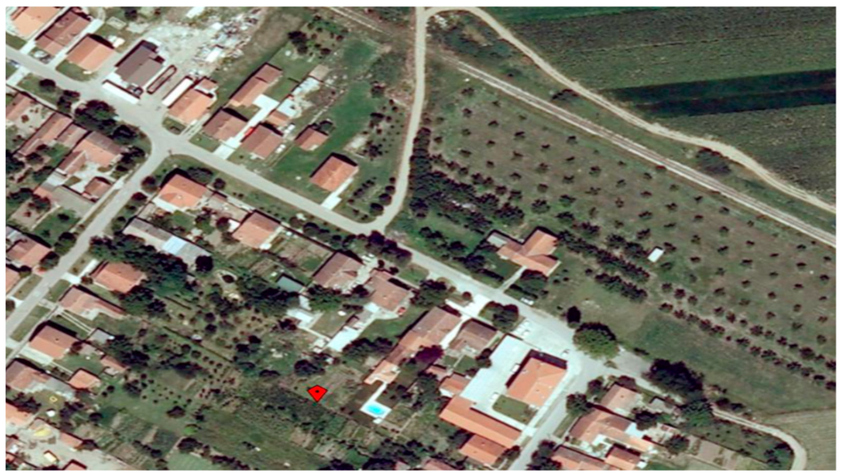
Figure 7.
Forecasts from the SARIMA model for the the air temperature time series.
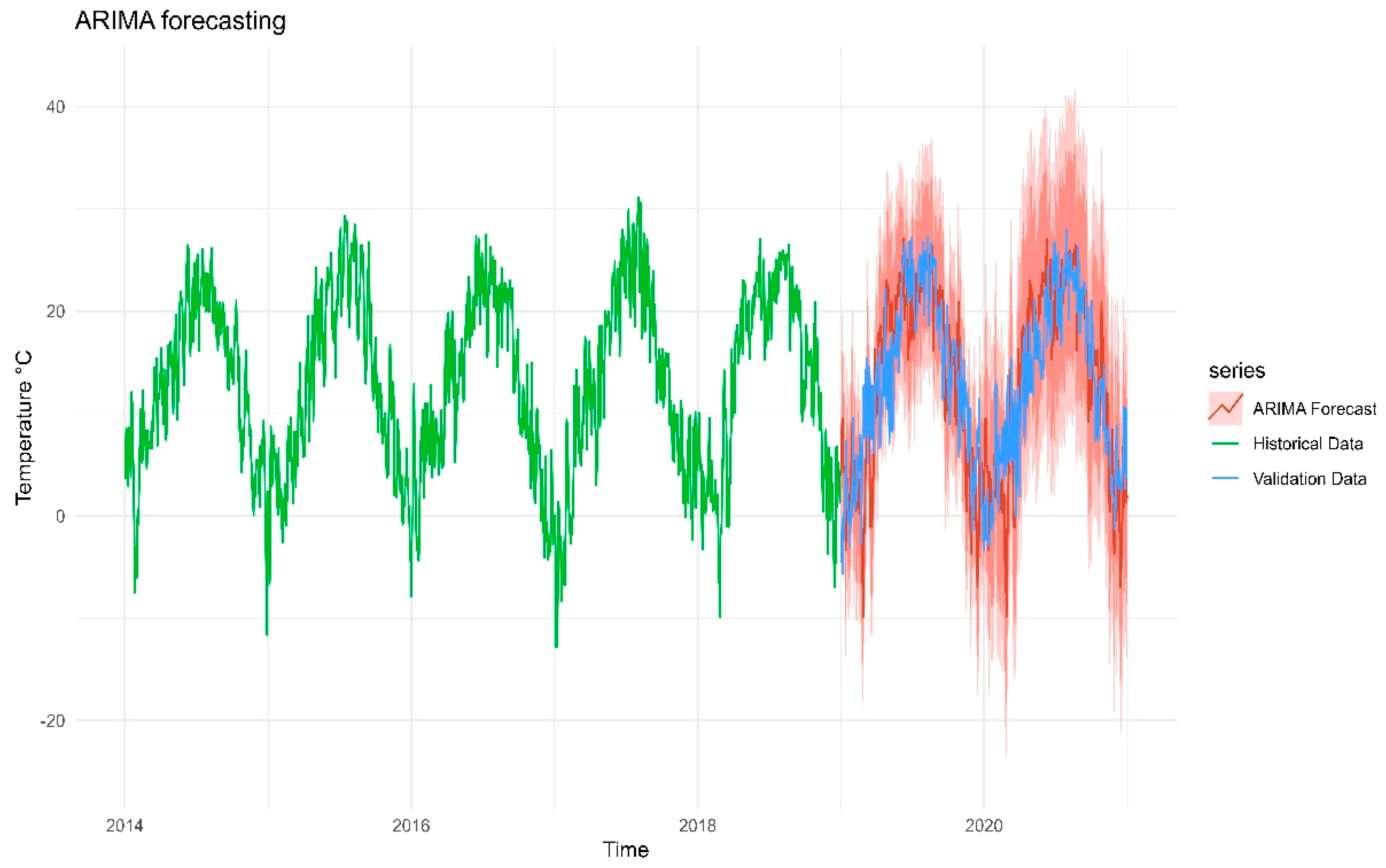
Figure 8.
Forecasts from the ARIMA model for the precipitation time series.
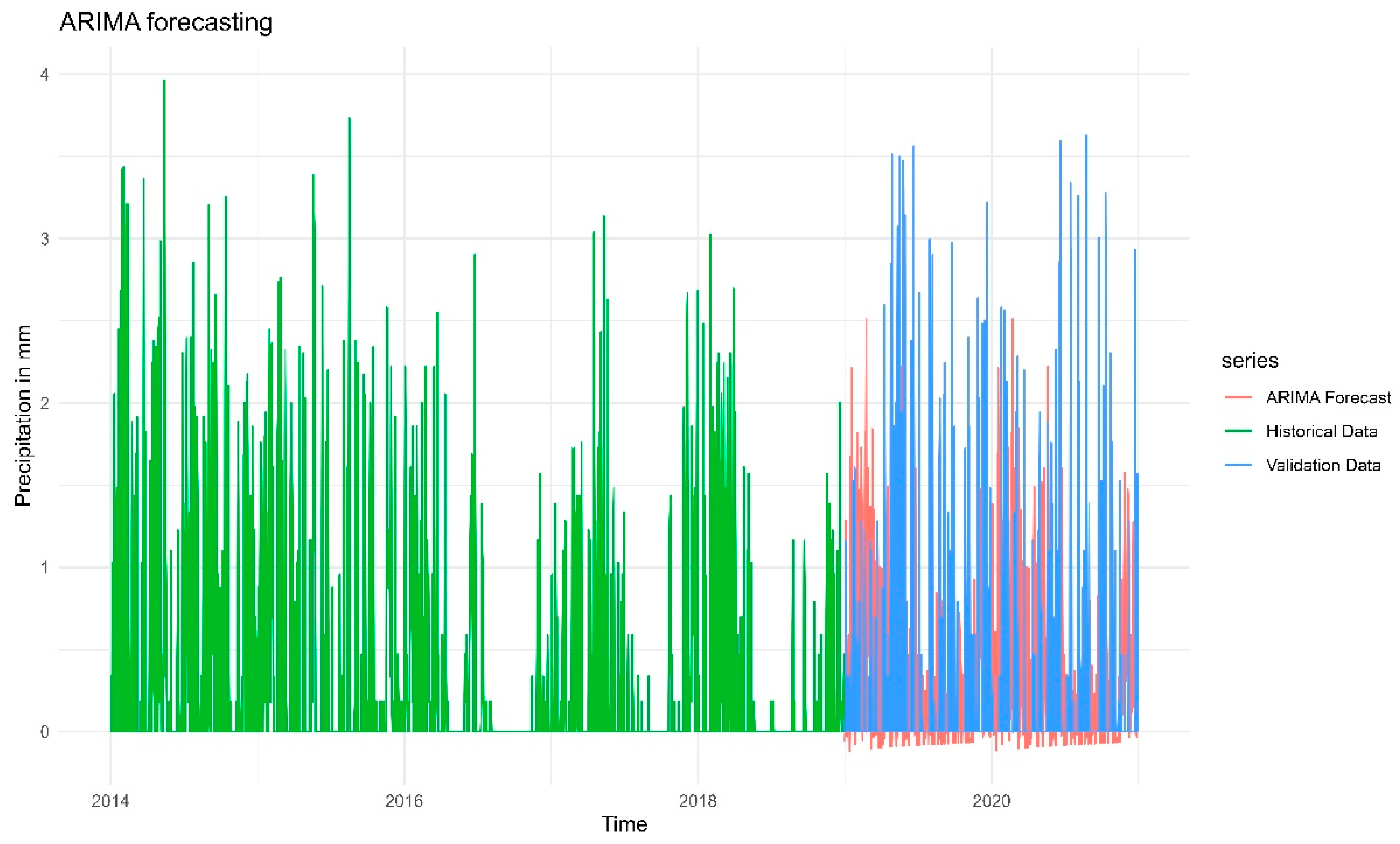
Figure 10.
Forecasts from the ARIMA model for the wind speed time series.
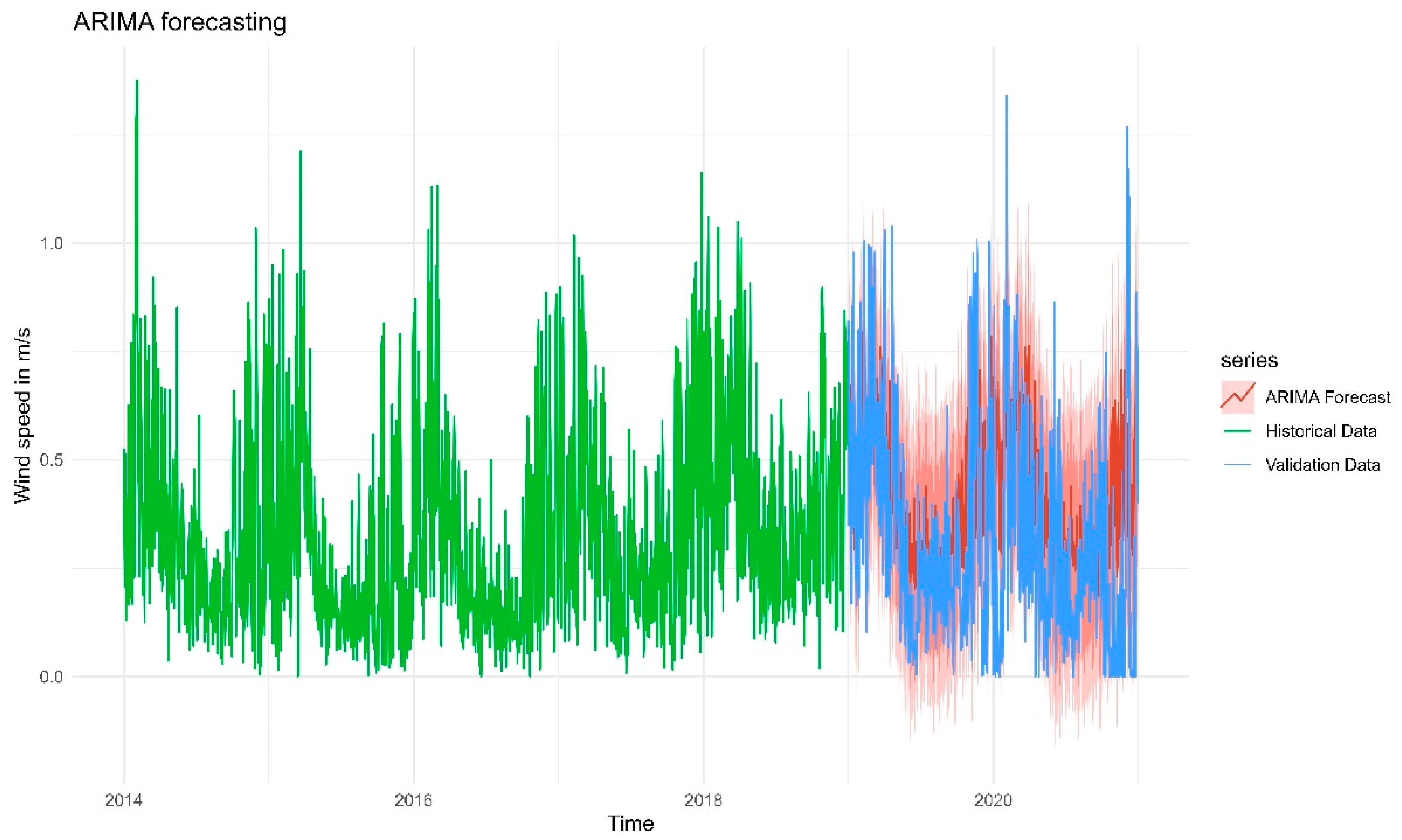
Figure 11.
Forecasts from the Holt-Winters additive method for the the air temperature time series.
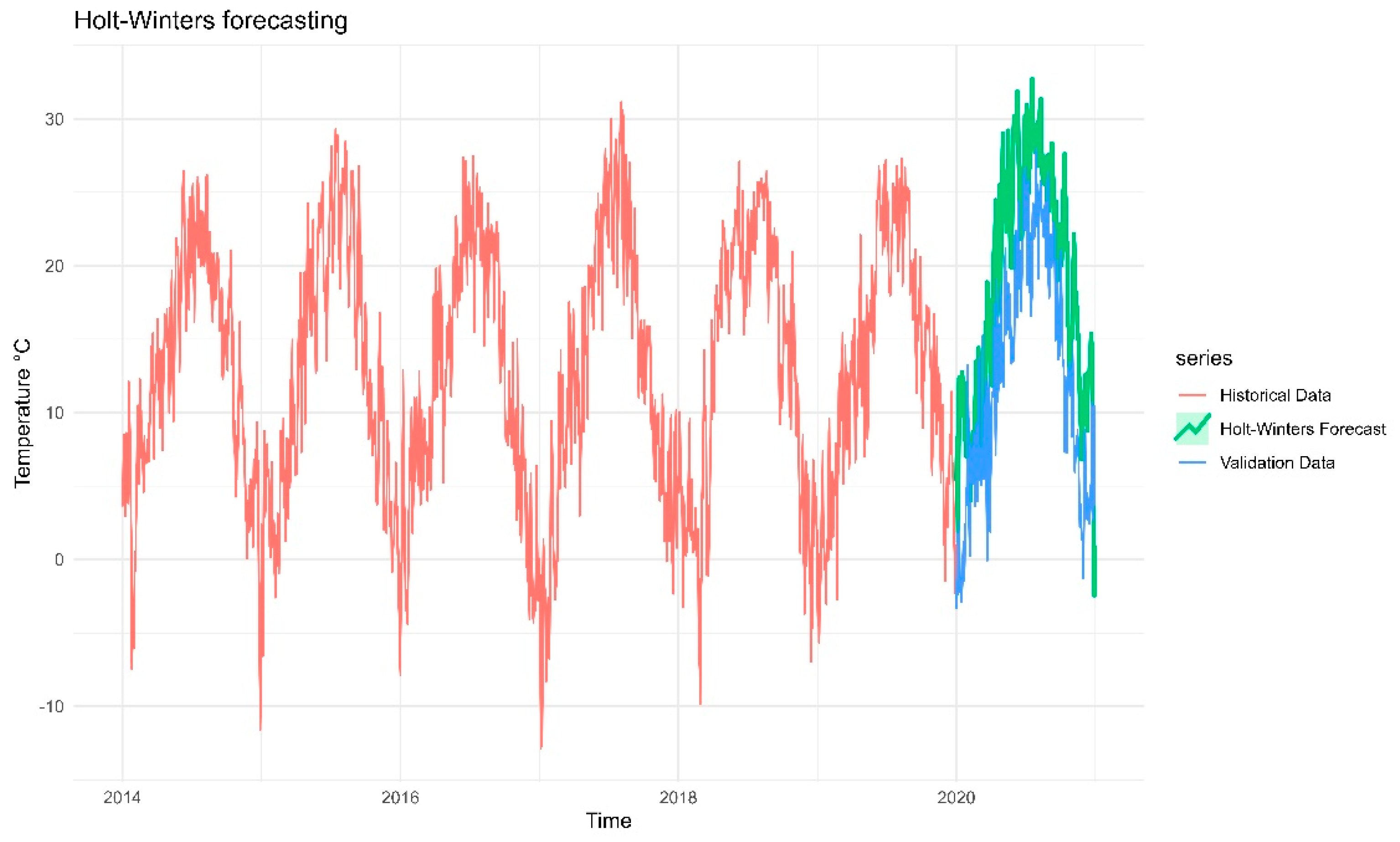
Figure 12.
Forecasts from the Holt-Winters additive method for the log-transformed daily precipitation time series.
Figure 12.
Forecasts from the Holt-Winters additive method for the log-transformed daily precipitation time series.
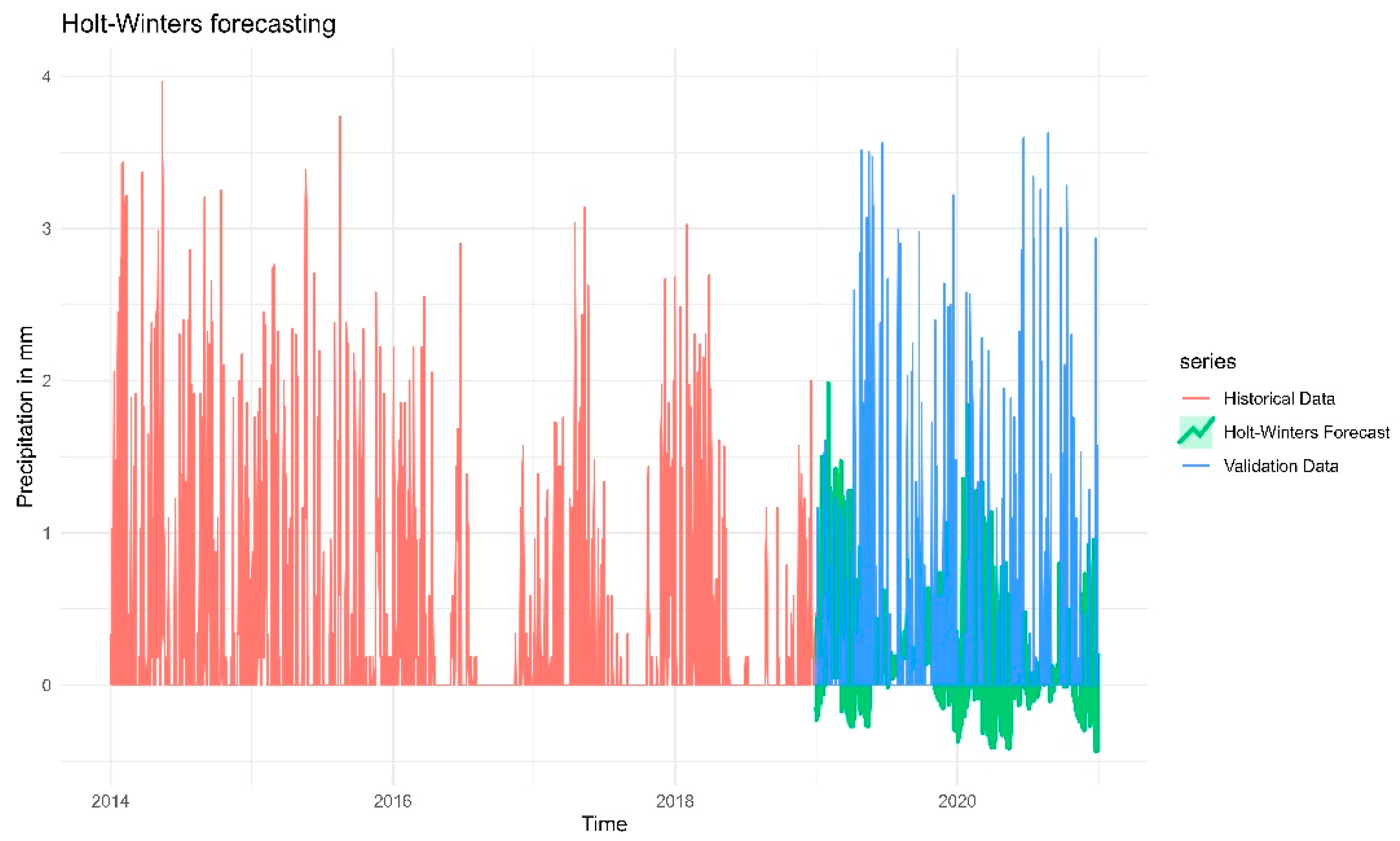
Figure 13.
Forecasts from the Holt-Winters additive method for the log-transformed daily soil moisture time series.
Figure 13.
Forecasts from the Holt-Winters additive method for the log-transformed daily soil moisture time series.
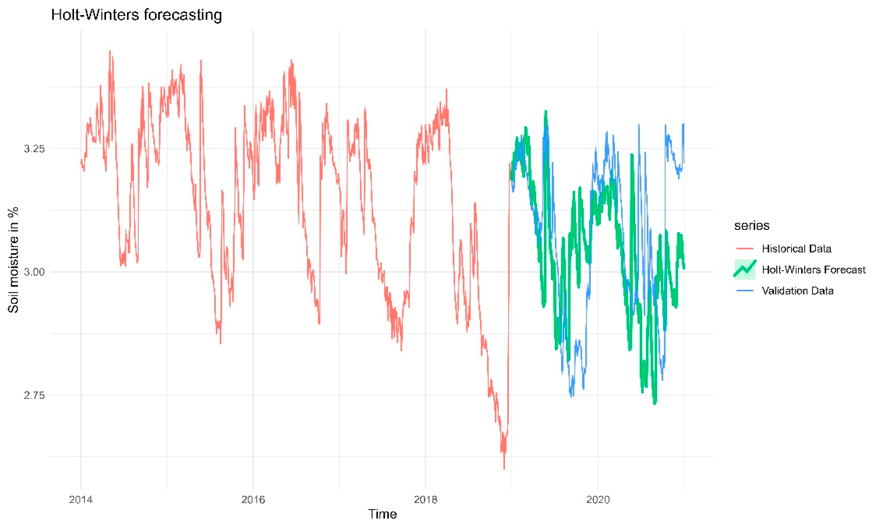
Figure 14.
Forecasts from the Holt-Winters additive method for the log-transformed daily wind speed time series.
Figure 14.
Forecasts from the Holt-Winters additive method for the log-transformed daily wind speed time series.
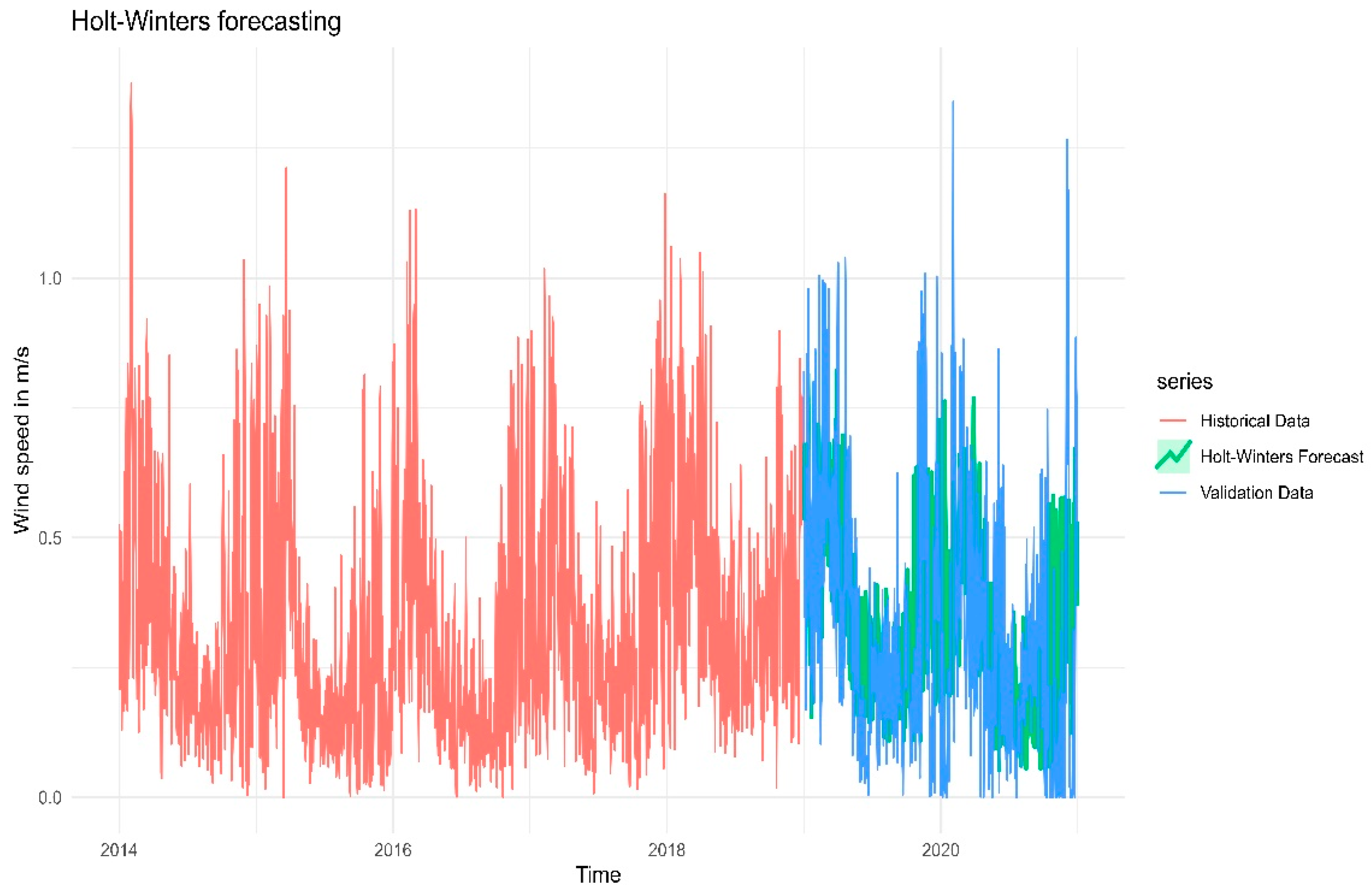

Table 1.
Data structure.
| Attribute name | Description |
|---|---|
| Time | Date and time of the value |
| Device | Device identification number |
| ID value | Sensor identification number |
| Value | Measured value of the parameter |
Table 2.
(S)ARIMA models and their criteria values, for all three time series.
| Time series | Model | AIC | AICc | BIC |
|---|---|---|---|---|
| Temperature | ARIMA (3,0,0)(0,1,0)[365] | 7430.99 | 7431.01 | 7452.13 |
| Precipitation | ARIMA (5,1,3) | 2986.24 | 2986.33 | 3035.81 |
| Soil moisture | ARIMA (3,0,0) |
2507.79 |
2507.82 |
2535.34 |
| Wind speed | ARIMA (3,1,2) | -1689.37 | -1689.32 | -1656.31 |
Table 3.
Information criteria of the Holt-Winters models for all four time series.
| Time series | AIC | AICc | BIC |
|---|---|---|---|
| Temperature | 13236.42 | 13236.44 | 13253.50 |
| Precipitation | 4756.21 | 4756.22 | 4772.74 |
| Soil moisture | -5093.26 | -4844.32 | -3147.94 |
| Wind speed | 453.38 | 702.31 | 2398.70 |
Table 4.
Accuracy performance indicators of both models for air the temperature time series.
| Measure | ARIMA (3,0,0)x(0,1,0)[365] | Holt-Winters |
|---|---|---|
| MAE | 1.918 | 2.168 |
| RMSE | 2.748 | 2.953 |
| MAPE | 55.856 | 66.882 |
Table 5.
Accuracy performance indicators of both models for the precipitation time series.
| Measure | ARIMA (5,1,3) | Holt-Winters |
|---|---|---|
| MAE | 0.374 | 0.467 |
| RMSE | 0.545 | 0.730 |
| MAPE | Inf | Inf |
Table 6.
Accuracy performance indicators of both models for the soil moisture time series.
| Measure | ARIMA (3,0,0) | Holt-Winters |
|---|---|---|
| MAE | 0.276 | 0.017 |
| RMSE | 0.479 | 0.032 |
| MAPE | 1.215 | 0.568 |
Table 7.
Accuracy performance indicators of both models for the wind speed time series.
| Measure | ARIMA (3,1,2) | Holt-Winters |
|---|---|---|
| MAE | 0.113 | 0.156 |
| RMSE | 0.151 | 0.219 |
| MAPE | Inf | Inf |
Disclaimer/Publisher’s Note: The statements, opinions and data contained in all publications are solely those of the individual author(s) and contributor(s) and not of MDPI and/or the editor(s). MDPI and/or the editor(s) disclaim responsibility for any injury to people or property resulting from any ideas, methods, instructions or products referred to in the content. |
© 2025 by the authors. Licensee MDPI, Basel, Switzerland. This article is an open access article distributed under the terms and conditions of the Creative Commons Attribution (CC BY) license (http://creativecommons.org/licenses/by/4.0/).
Copyright: This open access article is published under a Creative Commons CC BY 4.0 license, which permit the free download, distribution, and reuse, provided that the author and preprint are cited in any reuse.


