
Submitted:
23 April 2025
Posted:
24 April 2025
You are already at the latest version
Abstract
In most cases, the sizes of the daughter cells of diatoms follow the MacDonald-Pfitzer rule, whereby in many species all diatoms divide once in each generation. In contrast, there are division schemes in which the smaller or larger daughter cell is delayed in its division by one generation and therefore lead to Fibonacci growth. Several properties of diatoms, especially in chain-like colonies, that exhibit such delayed division can be modelled by Lindenmayer systems. These include, above all, the size and orientation of the diatoms. Certain sequences of properties, such as the differences in size indices of neighboring diatoms, are aperiodic and represent self-similar fractal structures. For the division schemes studied, explicit solutions can be found for the number of diatoms of a certain size in each generation. For the experimental differentiation of the division schemes in a diatom chain, in addition to the observation of the division processes over several generations, methods are available that only require the analysis of the structure of a sufficiently large sample. This includes the investigation of the differences in the sizes of neighboring diatoms, the orientations of the diatoms and the frequencies of size indices in a culture.
Keywords:
diatom
; MacDonald-Pfitzer rule
; Lindenmayer system
; Fibonacci growth
; delayed cell division
; chain-forming diatoms
; size sequence
; fractal
1. Introduction
Diatoms are an ecologically important class of unicellular algae that can be found in almost all aquatic systems and in terrestrial environments. Diatoms have a hydrated silica exoskeleton consisting of two halves of different sizes, the hypotheca and the epitheca. The epitheca overlaps the hypotheca. Each theca consists of a valve, which varies in shape depending on the species, and a number of associated silicate girdle bands. A detailed description can be found in Round, Crawford and Mann [1].
Diatoms reproduce predominantly by vegetative division. As early as 1869, Macdonald [2] and Pfitzer [3] recognized in the diatoms they studied that during such cell division, the epitheca of the mother cell becomes the epitheca of the larger daughter cell and the hypotheca of the mother cell becomes the epitheca of the smaller daughter cell. For each theca of the mother cell, a slightly smaller theca is formed. This results in one cell the size of the mother cell and one smaller cell. This rule has been confirmed in many species (e.g. [4]), but exceptions are also known [5]. When a minimal size is reached, sexual reproduction occurs, resulting in one or more large initial cells. There are also species that can restore their size by vegetative enlargement (see [6] for a review).
Macdonald and Pfitzer assume in their considerations that there is a uniform doubling time. The larger and smaller daughter cells divide simultaneously and therefore the number of diatoms in each generation doubles. Such a division behavior of a species, which follows the McDonald-Pfitzer rule, is referred to here as the P-model.
In the following, the generation is numbered with the index n, whereby the development should begin with a single diatom at . In the literature there are also generation counts starting with 1. In the context of cell size reduction for the morphological category of pennates (bilaterally symmetrical), the size of a diatom is understood to be the apical length. In the morphological category of centrics (radially symmetrical), the diameter of the circumcircle can be used. This length is characterized by a size index k. The value corresponds to the cell of maximum size. With each reduction step, k is incremented until the maximum value is reached, i.e. the size at which a cell enlargement is required. Using the notation for the number of diatoms with the size index k in the n-th generation in the P-model it follows from Macdonald-Pfitzer's rule for :
It is known from Pascal's triangle that:
Without taking mortality processes into account and for diatom sizes above the threshold for the necessity of cell enlargement, the size classes are given by binomial coefficients. An early study applying this result to diatoms can be found in Richter [7].
Otto Müller observed a delayed vegetative division in certain diatoms in the chain-forming Ellerbeckia arenaria (Moore ex Ralfs) R.M.Crawford 1988 (basionym Melosira arenaria D.Moore, see [8]). He names the epithecae with the letter f, the hypothecae with u, so that a diatom in a chosen horizontal position is named by a pair fu or uf. In his publications from 1863 [9] and 1864 [10], he distinguishes between valves with and without thickening for the species under consideration (Figure 1a) and places a small circle under the letter if the valve has no thickening and a line otherwise, so that the combinations and their mirror patterns result. For details of the morphology, see [11].
Figure 2 shows an illustration of a chain from [10]. The girdle bands are marked by red lines. Each is connected to the larger valve of the diatom and points to a neighboring thickening.
If two diatoms in the chain have their larger valves next to each other, their girdle bands will point away from each other. There are no girdle bands that cover the valves of the two groups at their point of contact, which makes them visually separate. Otto Müller was able to show that this divides a chain into groups of two diatoms (sets of twins) or three diatoms (sets of triplets). In Figure 2, these groups are combined by horizontal brackets placed above the chain.
In all cell divisions, Otto Müller observed the transitions shown in Figure 1b. The valves of the parental cell keep their structure. For details, please refer to [9,10,12]. Regarding the temporal development, it is essential that there is a delayed division, which Müller shows exemplarily for a chain of three diatoms (Figure 1c). According to the rule in Figure 1b, he deduces from this sequence back to a single starting cell , whereby the smaller daughter cell , which has inherited the hypotheca ( becomes ) from the mother cell, skips a division. In the next generation step, it divides again. According to Müller, such a skipping of one division of the smaller daughter cell occurs in all structures shown in Figure 1b. This implies asymmetry in the division behavior. Such behavior is referred to below as the M-model. Based on the illustration in [13], Figure 3 shows the first three subsequent generations of the development of a diatom chain starting with .
The valves of newly formed cells that will not divide in the next step, i.e. are in an interim state, are indicated by blue valves. The grey shapes between the generations visualize the mapping of mother cells to daughter cells. The numbers in these figures are the size indices of mother (top) and daughter cells (bottom), assuming that development began with an initial cell. Due to the skipping of divisions, the number of diatoms does not grow exponentially. This will be discussed in more detail later.
The third generation consists of a set of triplets followed by a set of twins, each with overlapping girdle bands. When drawing the development for the following generations, it becomes clear that the entire chain consists of these two groups.
A surprisingly different observation was made by Laney, Olson, and Sosik [14] on Ditylum brightwellii using time-lapse imaging. They report that the daughter cell that inherits the hypothecal frustule divides in each generation. However, the division of the larger daughter cell is delayed in comparison. This model is subsequently denoted as the L-model. In an idealized approach, in which exactly one division is skipped, the L-model and the M-model form a pair of opposites regarding division behavior. For further details, particularly on the temporal behavior of the development, see [13,15].
The structure of a chain-like colony whose diatoms divide according to the McDonalds-Pfitzer rule, in particular the size sequence of the diatoms and the number of diatoms of a certain size at a given generation obviously depend on the model of division. In this work, the properties of such chains and the distribution of sizes will be studied for the presented models. The background to this question is the possibility of investigating the division behavior of a species under consideration. Direct evidence of delayed division requires an observation period on the order of several generations. It should be borne in mind that the question arises in the case of chain-like diatoms, other diatoms living in colonies and individual diatoms. Motility complicates observation. On the other hand, easily testable criteria require the fulfilment of certain conditions, in particular sufficient synchronicity of division processes and the negligibility of death processes within the examined sample.
2. Materials and Methods
2.1 Synchronicity
Chronological sequences of patterns, such as those shown in Figure 1c and Figure 3, are referred to as generations in the literature cited (e.g. [13]), although not all diatoms divide in the time interval between these snapshots but skip a doubling period. This convenient counting method will also be used here. However, restrictions and limitations of this representation should be pointed out.
A description of the processes, as given by O. Müller [9,10], is implicitly based on the assumption of equal doubling times, whereby the doubling time is understood as the period between successive vegetative cell divisions. In the case of cells that skip a division, the double interval is assumed. It is known that doubling times and thus also the generation time, which is defined as the mean doubling time, depend on environmental parameters such as light intensity, nutrient concentration or temperature (see e.g. [16]). Even under constant environmental conditions, the doubling time is a random variable that has a natural statistical range of variation and can be described by a density function [17]. In the case of the M-model and L-model, there are therefore two distributions, one for division without delay and one for division with delay.
The stochastic character of the doubling times leads to a temporal drifting apart of the divisions in a culture. When starting a clonal culture with a single cell, after many divisions you will encounter a wide variety of division stages occurring simultaneously. For the applicability of the given considerations and the visualization of the generations of a chain, it is essential that the width of the distribution, e.g. measured as the standard deviation, is small compared to the generation time. The smaller this ratio is, the longer a real colony as shown in Figure 2 can grow, which corresponds to the theoretical structure resulting from the stepwise application of the rules in Figure 1b. Observations and quantitative considerations on the synchronicity of divisions in diatom chains can be found in [18,19].
It should be mentioned that cell divisions of diatoms can be synchronized by varying environmental parameters periodically. This can be achieved by periodic changes between phases of high and low light intensity [20,21,22,23]. Periodic addition of silicate to colonies that are kept under silicate deprivation can also be used for synchronization [24,25]. Provided they can be successfully applied, these methods offer the fundamental possibility of studying chain-like diatom colonies over many generations.
2.2 Lindenmayer systems
A Lindenmayer system (L-system) is a mathematical formalism developed by Aristid Lindenmayer that is particularly suited to modeling the growth processes of plant development [26,27]. It is a triple consisting of:
- Alphabet
- Replacement rules (rewriting rules or productions)
- Initial sequence ω (axiom)
The alphabet is a set of letters. The term "letter" is broadly defined, as a letter can also contain indices and thus numbers.
The formalism starts with the initial string ω, a sequence of letters of the alphabet. The replacement rules are applied to this string. By replacing individual parts (individual characters, substrings), a new string of letters of the alphabet is obtained. The application of the replacement rules is continued iteratively, so that a sequence of such strings is created. In the following, a generation of a chain-like diatom colony is simply understood as the associated string.
Koster and Lindenmeyer successfully used an L-system to describe the positions of heterocysts in a filamentous colony of the cyanobacterium Anabaena catenula [28]. As a one-dimensional system is described here, the term “one-dimensional L-system” is used. L-systems allow the treatment of structures of plants with complex branching, which enables the generation of computer-generated images of plants [29]. In the context of diatoms, a one-dimensional L-system can be used to determine the position of connection points in zig-zag-shaped chains of Diatoma vulgaris [19]. Of importance for the study presented here is the fact that the size sequence of diatoms in a chain-like colony can be modeled by an L-system. This approach is described by Ussing et al. [30]. The authors assume that Macdonald-Pfitzer's rule is applicable and that all cells divide synchronously. The resulting sequence was analyzed in [18].
It is remarkable that Otto Müller [9] defined an alphabet with the abbreviations and specified substitution rules (Figure 1b). These can be understood not only at the level of pairs of letters of an alphabet, but also as replacement rules for single frustules. The only missing extension for a complete description as an L-system is one that allows the delayed division shown in Figure 1b to be included in the calculation scheme.
3. Mathematical treatment
3.1 The Müller model as a Lindenmayer system
3.1.1 Alphabet
Whereas Müller bases his alphabet on the frustule as the smallest structure, here a single diatom is represented by one letter of the alphabet in order to achieve a uniform representation for all the division models. This letter should have the form , where When the larger valve is on the left, it is labeled L or l; when the larger valve is on the right, it is labeled R or r. For modeling the delayed division of the smaller daughter cell, a distinction must be made between cells that can divide immediately and cells in the interim state. Cells that can divide within a doubling time are labeled with capital letters (L or R), cells in the interim state with lower case letters (l or r). In addition to the four possibilities for diatoms shown in Figure 1b, their mirror image forms (large valve on the right) must also be considered. As the size sequence of the diatoms in chains is to be studied, the size index of their larger frustule is added to each letter as a superscript number k. Thus, should denote a diatom whose left valve is larger than its right valve, which can divide immediately and has the size index k. The index j is used to assign a structure to the diatom as shown in Figure 1b. Diatoms in the interim state, but otherwise with the same characteristics, are named . The mirror-image diatoms are correspondingly and . The assignment to the structures can be found in Table 1.
Although the size index has a maximum value kmax in nature, this is not relevant for the following considerations, so that the alphabet is defined by the set:
The alphabet takes into account size index (S), orientation (O) and valve structure (V). By removal of information like the structure index or size index, simplified alphabets can be obtained for limited considerations.
3.1.2 Replacement rules
When forming a generation, each letter of the previous generation is replaced by one or two letters of the alphabet. Consider the replacement rule of as an example.
has the structure . The size and structure of its larger daughter cell is identical according to Figure 1b, so that it is described as like the mother cell. The smaller daughter cell exhibits the structure and has structure index 2 according to Table 1. Its larger valve is on the right, and it is in the interim state, which is why it is written with a lowercase letter. Its size index is incremented because it is the smaller daughter cell. It divides with a delay of one generation and is thus described by . The following applies:
The memory is modeled by the intermediate step. All other productions are determined by an analogous procedure. For the diatoms with the large valve on the right, the replacement rules can be found by mirroring. All replacement rules are summarized below.
As these replacement rules exactly determine the next generation and the neighborhood of a diatom is not included in the rules, this L-system is deterministic and context-free and is therefore referred to as a D0L-system.
- If we start the development with the axiom and denote the string of the nth generation by , this generation sequence results for :
corresponds to Figure 2, which indicates the same starting value. In this generation, all the diatom structures according to Figure 1b appear for the first time. As the L-system is context-free, each diatom develops into a structure in the same generation sequences that would have resulted if it had been chosen as an axiom. For example, from in , a subtree arises in subsequent generations, as it would have formed with the axiom . As mentioned, this can also be mapped to the axiom by lowering the size indices by the value 2.
3.1.3 Introduction of operators and alternative algorithm for calculating generations
In the following, an equivalent formulation is chosen for the replacements [18]. The productions are expressed by an operator P. The substitution rules assign the string to the letter g of the alphabet. Parentheses are not required for an operator. They are used here to indicate the range of the operator. The first substitution rule in (6) can be written as:
Thus the nth generation of the axiom is expressed by . As the L-system is not context-sensitive and therefore each character is replaced separately, the following is valid when applying P to a string G:
Furthermore, the operator S is introduced, which mirrors the string including its elements.
To mirror the characters of the alphabet, use the structures defined in Table 1 or the verbal description. The following applies for all j:
It is easy to convince yourself of the commutativity [18]:
If you change the view of a diatom chain from top view to bottom view, you will see the mirrored chain. If you determine the next generation by applying the replacement rules, you get the mirrored next generation. The same result is obtained if you first determine the next generation and then change the view, i.e. mirror it.
Finally, an operator I is defined which increments the size indices of all diatoms in a string:
Whereby:
As already stated, the boundary k < kmax is not explicitly considered. These commutator relationships are valid as the operator I only affects the size indices:
3.1.4 Reformulation of the algorithm
- The operators make it possible to reformulate the algorithm for calculating subsequent generations.
Theorem 1.
For and the following applies:
Proof of Theorem 1.
By applying the substitution rules, the context independence and the commutator relations, we obtain the following for :
Each generation can be created by recursion from a previous generation and a second previous generation, without explicitly applying the replacement rules to each character of the string. The calculation scheme for calculating for consists of concatenating the stings and according to equations (18). The generations resulting from the axiom are obtained by mirroring.
As Otto Müller [9,10] points out, the lengths of the generations are given by the Fibonacci sequence. Defining the Fibonacci sequence by , and then the number of letters in equals fn+2 because of the lengths of the first two generations and equations (17). Note that the I and S operators do not change the length of a string.
3.1.5 Restriction to orientation and size index
The division rule, according to which the smaller daughter cell divides with a delay, is not fundamentally linked to a specific structure with thickenings. This information is now omitted and only the size indices and orientations of the diatoms are considered. The index describing the thickenings is thus dropped and the alphabet is reduced to:
The replacement rules become:
In the generation sequence (7), only the subscripts have to be removed. Instead of the four equations in (17), we find for :
A generation is obtained by concatenating the previous generation with the mirrored and incremented second-last generation. Each generation is the beginning of the next.
It should be remembered that the axiom was used as axiom here. If you want to get the generation sequence for the axiom , you just have to mirror , because . If you want to obtain an expression for the sequence of generations for the axiom analogous to (21), apply the mirror operator to both sides of this equation. Using the notation , you get . Each generation is the end of the next.
A higher size index in the axiom () causes a corresponding increase in all indices, because . If you want to start the development with an interim state, only one additional step, i.e. one generation time is required to achieve the described generation sequence. In this sense, the alternative description of the L-system (21) is complete. The same procedure can be followed for the other L-systems in this work if you want to change the axiom.
The recursive structure in equation (21) enables a representation in which only depends on . Using equation (21), applies. As forms the first part of with the length , this string can also be taken from when calculating according to (21). This is shown graphically in Figure 4.
This means that can be determined from alone. This is indicated by the grey arrow at the bottom of the figure.
As can be seen in generation , the sequence can also be regarded as consisting of three strings, with the middle one from generation being created by applying IS. The whole generation is mirror symmetric if the size indices are neglected, except for this middle string. This is mentioned in [13] for the example of the 5th generation shown in the paper.
3.1.6 Size indices
According to the alphabet, each generation contains information about size indices and orientations, including interim states. One can go a step further and focus on orientations including the interim states or on size indices. Restricting to size indices, each generation can be written as with . The size index is the j-th element in the generation n. The alphabet is reduced to . Expression (21) is still applicable. The mirror operator only changes the order, but not the values. In terms of size indices, (21) can be rewritten as
According to the note above, for , the values of generation contributing to generation can also be taken from generation n.
3.1.7 Sequence of differences and fractal structure
As the absolute assignment of a measured size to a size index is not straightforward, the difference sequence of the size indices is of particular importance. This is discussed in more detail below. The difference sequence of a generation is defined for by a sequence of integers
where i takes the values . The string has the length . Using (22) yields for :
As can be quickly verified, the difference between the first value of the second subsequence and the last value of the first subsequence is always equal to 1. Again, the self-similarity of the sequences allows the differences from generation that contribute to generation to be taken from generation n for . In compact notation, (24) can be written as follows for
where the upper bar is meant to indicate the inversion of all signs. The first five generations read:
The values 1 for are shown in bold.
When looking at the difference sequence, it is striking that only the values -1, 0 and 1 occur in it. The proof that this applies to all generations can be done by induction (for the proof technique, please refer to textbook [31]). , in which all stated values occur, is taken as the base case. The induction step uses the fact that the range of values {-1, 0, 1} is not changed when applying the iteration described in (24) and (25). It should be noted that for division rules without delayed division (P-model) only the differences -1 and -1 occur, but not the value 0 [18]. There are no neighboring diatoms of the same size in the P-model.
The sequences according to equation (21) cannot become periodic as the generation index n increases, because the maximum size index increases continuously as a result of incrementing. Appendix A shows that the sequences of differences do not become periodic either.
It is known that self-similarity and fractal structures are typical for Lindenmayer systems [29,24]. In a P-model, the sequence of differences can be visualized as a dragon curve [18]. To do this, a line with a unit length is first drawn in the manner of a turtle graphic. A rotation is then performed for each element of the sequence, the size of which depends on the value of the element, and then a step is taken forwards by the same unit of length. The dragon curve is obtained by performing a 90° rotation in a clockwise direction for the value +1 and a 90° counterclockwise rotation for the value -1. The following applies to the generations of size differences in the P-model [18]:
A curve segment of the same length is added to the existing curve after rotation by 90° (value 1). There is self-similarity, in particular is similar to . For details on the dragon curve, please refer to Tabachnikov [32].
In the case of the M-model, there are three different values for size differences. An appealing visualization of the sequence can be obtained by proceeding similarly to the dragon curve but choosing an angle of 120° and not performing a rotation for the value 0, i.e., appending just one step of one unit of length in the same direction. The result is shown in Figure 5.
Each sequence is assigned a different color. The size of the curves does not double from generation to generation but follows the Fibonacci sequence. For the next generation, curve segments of different lengths are combined. Each generation is similar to every other generation, which can be seen by scaling them to the same size and aligning them in the same direction.
3.1.8 Orientations
The orientation and the interim states can be described by a simple L-system and can be computed independently of the size indices. We restrict ourselves to the alphabet . For example, L can be chosen as the axiom. The substitution rules follow directly from (20) to give . Equation (21) can still be used, only the increment operator is no longer needed, i.e. , where the letter J has been chosen for the generations of orientations. The mirroring is done according to the rules (11), where the size index is irrelevant.
The sequence of orientations is not periodic, which does not immediately result from what has been said so far. The proof follows the scheme of the proof for the sequence of differences (Appendix A). The number of occurrences of a letter of the alphabet in generation n is not given by a Fibonacci number. Therefore, for a generation n, consider the number of all lowercase letters (l, r) and the number of all uppercase letters (L, R). The operator S does not replace lowercase letters with uppercase letters, i.e. this number is invariant when S is applied. From we can see that these numbers have Fibonacci growth. Taking into account the initial conditions, we obtain and . The ratio converges to an irrational number for , which would not be the case if the sequence were periodic.
The sequence as seen in (7) can be visualized by a fractal curve if one chooses a rotation angle and assigns certain multiples of this angle to the characters of the alphabet. With a P-model there is an alternating sequence of right and left orientations [18]. Aperiodicity and a fractal structure therefore do not occur.
3.1.9 Sets of twins and sets of triplets
Sets of twins and sets of triplets are characterized by free thecae at both ends [9,10,13]. This property is retained when mirroring and incrementing are applied. Since structures of sets of twins and sets of triplets arise from a single cell, every chain that develops according to O. Müller's model consists exclusively of a sequence of these two structures. It is not surprising that this sequence can also be described by an L-system. In contrast to the systems presented so far, the objects here do not stand for a single diatom, but two or three diatoms. It can be seen in (7) that a set of twins becomes a set of triplets in the next generation and then the set of triplets becomes a set of triplets and a set of twins. The order in which sets of triplets and sets of twins appear depends on the orientation of the set of twins with which the generation sequence begins. Consequently, orientation must also be taken into account in the alphabet. We denote a set of twins in the orientation as shown in (7) for the second generation (structure Lr) with the letter T and its mirror image with . Correspondingly, a set of triplets as in the third generation (structure LrR) should be denoted by V and its mirror image by , so that the alphabet is given by
The production rules for the above specified structures result from to give
When starting the development with T, a set of triplets and a set of twins appear after two iterations, whereby the set of twins has the opposite orientation to the parent. To obtain the replacement rules for and , it is sufficient to mirror the rules for T and V. If we restrict ourselves to the axiom V without loss of generality (otherwise mirroring and/or executing an iteration step) and label the generations , we obtain analogous results to Theorem (21)
and thus
The similarity with the expression for the orientations is due to the fact that the replacement rule does not increase the number of objects and acts as a delay, even if the number of diatoms does not remain the same. The first generations are:
Again, there is Fibonacci growth with the length of equal to fn+2. The number of groups of twins grows with fn, the number of groups of triplets with fn+1, whereby the orientation was not considered, i.e. both orientations were grouped together. The evidence for non-periodicity presented in Appendix A is therefore transferable, considering the quotient of the number of groups of twins and groups of triplet groups.
3.1.10 Number of diatoms of the same size
For practical applications, it is important to know how many diatoms with a certain size index k occur in generation n. In Müller's model, this number is denoted by . If the development begins with a cell of maximum size (), then and . In the following generation there is again a cell of maximum size and a cell with the following size index, so that and . There are no further cells, thus . For the subsequent generations with , a recursion formula can be derived from (21):
The number of diatoms of size k in the generation has a part, which results from the identical repetition of the previous generation n and a second part, which originates from the second last generation . As all size indices are hereby incremented, the sizes contribute to this. It should be noted that there are no size indices smaller than zero and therefore no contribution to from generation . Therefore is defined. For one can immediately find that for any n.
To find the solution (33), you can iterate (32). For a chosen k as a function of n, a sequence of figurate numbers arises, which can be expressed by binomial coefficients.
Theorem 2.
The solution of the equation (32) for reads:
Proof of Theorem 2.
For and , the correspondence with the initial values is checked by inserting them into the binomial coefficient. Similarly, for and any n, (33) gives the value 1 in accordance with (32). Proof of correctness for is obtained by inserting it into the right-hand side of (32).
.
And therefore LHS=RHS. □
It is worth noting that all binomial coefficients can be found in Pascal's triangle. When this is left-justified, all solutions (33) for a chosen n are located on a diagonal. The sum of all binomial coefficients of a diagonal gives the Fibonacci numbers, as can also be seen from the recursion (32).
3.2 The Model according to Laney et al. as a Lindenmayer system
3.2.1 Notes on the model
At first glance, the M-model and L-model look very similar, so you might think that the results would be also very similar. However, this is only partly the case. The operators and methods introduced are fully applicable.
In the following, the same basic and partly simplifying assumptions are made, in particular the existence of synchronous divisions and a division delay of one generation for certain diatoms.
Valve structures and girdle band structures are not considered, so that the investigation is limited to sizes and orientations.
3.2.2 Alphabet and replacement rules
Because of the restrictions on size and orientation, the alphabet defined in (19) can be used. The replacement rules differ from those shown in (20) because the division of the larger cell is now delayed by one generation:
If the string for the nth generation at the start value is denoted by , then the L-system according to (34) yields this generation sequence:
Using the presented method, we find
and thus
The concatenation of the last generation with the second last generation results in a subsequent generation with the sum of the lengths and thus a Fibonacci growth. As in the case of the M-model, the length of is equal to fn+2. In contrast to and , however, no sequence is created in which the previous one is repeated, neither at the beginning nor at the end, so that the question of periodicity does not arise. The formation of a generation is shown in Figure 6.
As in Figure 4, a decomposition into three strings can be given.
3.2.3 Size indices
If we restrict ourselves again to the size indices with , it follows from (36):
3.2.4 Sequence of differences and fractal structure
The difference sequence of a generation for will also be given for this model. For this purpose, the differences with are formed using (37). For you get
The compact version with the notation used in (25), is as follows
These are the first five sequences:
The values 1 for are shown in bold. The range of values that differences can take on is larger than in the M-model and contains the values -2, -1, 1, 2. The proof is again by induction. Compared to the representation of the sequence of differences in the M-model, a different choice of angle proves to be favorable. In Figure 7, an angle of rotation of 60 degrees was chosen. With an absolute value of 2, two rotations are performed, i.e. one rotation of 120 degrees. Apart from that, the illustrations correspond.
Fractal structure and self-similarity are evident.
3.2.5 Orientations
If we consider only the orientations, i.e. restrict ourselves to the alphabet , the reduced substitution rules by , using the same axiom as for the M-model, lead to a non-periodic sequence . In recursive notation this sequence is given by . The first sequences are obtained from (35) by omitting the size indices.
3.2.6 Number of diatoms of the same size
The number of diatoms of a given size index k in generation n is also to be determined for the L-model. This is denoted by . The initial conditions for the calculation are identical to those for the M-model, i.e. , and . All other values in generations 0 and 1 are zero. The recursion for for is derived from equation (36) and gives
The diatoms of the same size from generation , as well as the diatoms of size index from generation n, contribute to the size index k in generation , since the latter are incremented according to (36). As there are no size indices smaller than zero, we again define .
To understand equation (41) it is helpful to imagine a 2-dimensional array with square cells and axes for n and k. As with a chessboard, color all cells black where is even and all cells white where is odd. The cells can now be assigned according to the initial conditions and equation (41). It follows from the recursion that only values from black cells contribute to a black array and only values from white cells contribute to a white array. The system consists of two distinct subsystems. In particular, this means that only the initial conditions from the same subsystem are included in the calculation of the values of a subsystem. In the recursion of the M-model (35), however, each value with depends on all initial conditions. These subsystems lead to a case distinction. To derive the solution to (41), consider the black and white marked fields separately. To restrict yourself to the black fields ( even), you can introduce new variables p and q by setting and . For the white fields ( odd), choose and . After some transformations you will find the solution (42).
Theorem 3.
The solution of the equation (41) for reads:
Proof of Theorem 3.
The proof is done by checking the conditions for the first two generations and inserting them into (41). Let us write (41) in the equivalent form and consider a cell with even. If we insert (42) into the right-hand side, we obtain
4. Results
4.1 Alternatives to long-term observations
When investigating the population dynamics of a diatom species, in particular the question of the validity of the McDonalds-Pfitzer rule arises. If this is fulfilled, which we will assume in the following, a simple division scheme without delay, one of the two models presented, or another scheme could be possible. An obvious option is to use long-term observation, that provides immediate information after a few division processes. This requires a sample that is vital over the observation period. A sufficient supply of nutrients and adequate light exposure must be ensured.
Long-term observations can also provide information without observing the individual division processes. The growth of a culture under consistently good conditions, i.e. in particular without depletion of nutrients and without decreasing exposure to light, can provide an indication of whether exponential or Fibonacci growth is present after measuring the size of the population. Ideally, the culture should be started with a single cell. To measure the population, an automated method using image analysis is recommended. A counting chamber can also be used for this purpose. Alternatively, biomass can be determined if samples are large enough. Whether the species forms chains is not important. As the Fibonacci sequence grows asymptotically exponentially, differentiation becomes more and more difficult as the number of generations increases. Measurement of the growth rate does not differentiate between the M-model and the L-model.
Other results already presented offer possibilities for analysis, especially on non-living samples and preparations. They therefore do not necessarily require cultivation of the species. The methods are explained below. They mainly refer to chain-shaped colonies. Synchronicity of cell divisions is only to be expected locally in such a chain, as it is lost after a few divisions among its descendants. In the tree structure of the divisions, starting from an initial cell, there are inevitably neighboring cells whose common ancestor dates back so many generations that synchronicity of their divisions is very unlikely. On the other hand, there are many sections that are sufficiently synchronous to allow analysis using the methods described. If we assume that the distribution of doubling times is so narrow that synchronicity over 5 generations is almost always given [18], a chain of at least diatoms is created in the P-model, which is likely to be consistent with theory. In one of the models with Fibonacci growth, there are only diatoms. Regardless of whether size differences, orientations or sets of twins and sets of triplet structures are examined, a loss of synchronicity must be expected for shorter chains. The shorter the range of a match with a theoretical sequence, the more likely it is that it is a random coincidence and the less informative it is.
4.2 Testing the applicability of the Müller model
A detailed description including the girdle band structure in chain-shaped colonies was only given for the Müller model. Whether this correctly describes the situation in a sample can be checked by placing an existing fragment of a chain in a defined horizontal position and expressing the visible structure as a string using the alphabet (3). If we restrict ourselves to the four types of the alphabet and their mirror images, i.e. ignoring the sizes, we obtain a sequence of orientations and thickenings. As it is not known at which point in the generation sequence the observed string occurs for the first time, it must be compared to the theoretical sequence according to (18) for a sufficient length. If there is no match, one must also search for the mirrored string in the theoretical sequence, as the chain has an orientation that is caused by the orientation of the initial sequence. Only a match is relevant, as there can be various reasons why no match is found. The model may be inappropriate, the recording may be incorrect or there may be a loss of synchronization. This statement applies analogously to all comparisons of recorded sequences with theoretical sequences.
The grouping of a chain into sets of twins and sets of triplets is based on the girdle band structure. It is easy to recognize visually. The procedure is analogous, the comparison is based on the alphabet and development as described in section 3.1.9.
4.3 Analysis of sizes and size differences
There is not necessarily a strict relationship between delayed cell division and the occurrence of thickenings, and the girdle band structure as described by Müller. To differentiate the division models without delay with delay, where the smaller or larger daughter cell can divide with delay, it is useful to examine the size sequence. However, it is difficult to assign a size index to measured absolute sizes. The reasons are
- There is natural variation in size even within the initial cell. This means that at best it is possible to give an interval for the size index in which the measured diatom is likely to fall.
- As this data is not systematically collected, it would need to be collected as a first step.
Although it turns out that incorrectly assigned size indices shifted by a fixed number also produce sequences that exist in the theoretical size sequence, an alternative is to examine differences between sizes and size indices. In this case, no uncertain large numbers appear in the sequences, but only the small differences. Even with this approach, differences in size must be assigned to differences in size indices.
As mentioned above, in the P-model the size indices between neighboring diatoms differ by only ±1 [18]. The frequencies of the length differences are then present in two peaks, with the scatter increasing with sample size due to the non-linear dependence of the size on the size index. To avoid errors due to loss of synchronization, it is important to ensure that the division stages are close together. The value range for the M-model additionally contains zero and, in the L-model the values +2 and -2 are included. This makes it possible to distinguish between the three models presented without analyzing the sequence, but it does not allow us to say whether another model describes the colony better. The advantage of the method lies in the simplicity of its procedure. As can be seen from the chains (26) and (40), all possible values occur even in short chains.
If a longer fragment of a chain-like colony with similar division stages is available, a comparison with the difference sequences according to (25), (27) and (39) is recommended. The significance of a match with one of these sequences increases with the length of the matching sequence. Once you have analyzed a fragment and assigned a difference value of the size indices to the size differences of neighboring diatoms, we look for this pattern or its mirror image in the calculated sequences. This sequence is similar to a part of a fingerprint being assigned to a location in a complete image. Since the difference sequence is self-similar, this assignment is not unique. If a sequence appears for the first time in a particular generation, it will also appear in subsequent generations due to the structure of the recursions. In all recursions, the number of fingerprint matches increases with the generation number, as a particular pattern is repeatedly appended and mirrored.
The feasibility of the method was demonstrated on a Eunotia sp., probably Eunotia glacialis Meister 1912 in [18]. In this species the length differences for adjacent size indices are around 1 µm and are therefore easy to measure. A colony of 25 diatoms was analyzed and found to be consistent with the P-model theory.
4.4 Analysis of the orientations
As shown, the sequences of sizes and orientations can be considered separately. It is useful to use the orientations of a clonal diatom chain as a fingerprint. The advantage of this is that it is not necessary to measure lengths quantitatively, but only to identify and record which diatoms have the larger valve on the left (l and L) or right (r and R). Since it must be assumed that it is not possible to distinguish visually between l and L or r and R, these characters are treated as identical when comparing the sample and the theoretical sequence. In a P-model, only the letters L and R exist anyway. It has been mentioned that they have alternating orientations.
4.5 Analysis of the size distribution
Measuring the lengths of many diatoms and classifying them in a histogram with subsequent comparison with theory takes a special place among the possibilities presented:
- One is not dependent on longer chain-like colonies but can also analyze short chains of a few diatom species, as well as diatoms that separate immediately after division.
- With an increasing number of diatoms, i.e. with a high generation index n in the sample analyzed, synchronism becomes less and less important. The reason for this is that the curves for the functions , and are similar as a function of k for closely spaced n (see below).
However, there are limitations and challenges:
- A culture started with a single diatom should be used as the basis, otherwise there will be a superposition of several distributions for the respective starting size.
-
The theory gives the number of diatoms for a size index, not the size. The comparison of the measurement to the theory therefore requires the assignment of the size to the size index.To compare the curve shapes, you do not need an exact assignment to a size index, as would be necessary for the comparison with the size sequence of chains, but a function as shown in [33,34] should be available to equalize the diagrams. If we consider the size indices at a given generation in a model without delay, then the theoretical frequency is given by (2). The binomial coefficients at a generation n, i.e. at a chosen measurement time, are symmetrical with respect to k. Apart from the fact that the size index 0 corresponds to the maximum size, this is not equivalent to a histogram of sizes due to the non-linearity mentioned above. However, symmetry is an important distinguishing criterion for the division models. To illustrate the characteristics of the distributions, the number of diatoms in the M-model and L-model are shown in Figure 8a for over k. The two models have the same number of diatoms in each generation, so that they can be visualized at the same scale.
In order to visualize the P-model together with the other models, one could limit oneself to normed values. To emphasize the quantitative difference of the entire population, a logarithmic representation was chosen in Figure 8b for values and all three models. The uneven heights in the L-model are characteristic, although they are less noticeable in the logarithmic representation. These discontinuities remain characteristic in later generations. Figure 8c corresponds to Figure 8a but has been calculated for . Although the maxima for . are about 6 orders of magnitude higher than those for , the similarity of the bar charts is striking. The corresponding logarithmic representation is shown on the right in Figure 8d.
The position of the maximum in the M-model is clearly shifted towards smaller size indices compared to the other models. However, the delayed formation of the larger daughter cell in the L-model does not lead to a corresponding shift towards larger indices. The maxima of the curves are at slightly lower k values in the L-model compared to the P-model.
4.6 Maximum size index
As explained at the beginning, no limitation of the size index has been introduced. However, there is a minimum or maximum size index at which cell enlargement becomes necessary. Whether this occurs through sexual reproduction, as is usually the case, or through vegetative reproduction depends on the species. A certain natural range of variation is presumably also given here, so that is not necessarily a well-defined value. In the context of size distributions, it should merely be noted that a certain size index is reached much earlier with the P-model compared to the M-model. The division behavior not only reduces the reproduction rate but also leads to a higher proportion of diatoms having a large valve size after the same period of development, i.e. the same number of generations. Species that divide according to the M-model significantly delay the onset of cell enlargement. As already discussed with reference to Figure 8, an analogous statement does not apply to the L-model, because the courses of the L-model and P-model are only slightly shifted with respect to each other.
5. Discussion
In view of the restriction of this mathematical modeling to the division process, the question arises as to the limitations and significance of the results presented here. Models for the development of diatoms, including their size can have different objectives. Models that are intended to describe the dynamics of the population over a longer period of time must include death processes as well as regularly occurring cell enlargement [13,15,34].
As the focus here is on the possibility of differentiating between the division models, only the growth phase starting from a single diatom is considered. The applicability is limited by the period of Fibonacci growth or, in the case of the P-model, exponential growth. This implicitly means a negligible mortality rate. This statement applies to the study of a fragment of a chain colony as well as to the size distribution of an entire culture.
Most of the concepts presented require a clonal chain-like colony. The need for a sufficient number of synchronous divisions in such samples was pointed out. Looking at the size distribution of a culture that has grown from a single diatom does not have these difficulties, because the characteristics of the distributions are almost independent of the generation. Loss of synchronicity means that the number of generations passed through is not identical but does not change the basic forms of the curves.
If it is not possible to assign a sample to any of the models considered, this may be due to the limitations of the method or its applicability to the sample (e.g. loss of synchronicity), but it could also indicate other possibilities that occur in nature. There is probably no principle that would prevent more than one generation being skipped during cell division, or the larger and smaller daughter cells dividing alternately with a delay. Delays of fractions of a generation time or random processes cannot be ruled out either. For the investigation of so far unknown division rules, direct observation of the processes is the method of choice.
The complexity of the systems studied, in particular the fractal structures, represent emergent properties resulting from the elementary rules of L-systems. They demonstrate the role of fractal structures in nature. However, in the context of the study of occurring patterns, they are less important than locally testable properties, such as the range of values of differences in size indices or shorter sequences of orientations.
Funding
This research received no external funding.
Conflicts of Interest
The author declares no conflicts of interest.
Abbreviations
The following abbreviations are used in this manuscript:
| P-model | Cell Division model without delayed divisions |
| M-model | Cell division model in which the smaller daughter cell divides with a delay. |
| L-model | Cell division model in which the larger daughter cell divides with a delay. |
| L-system | Lindenmayer system |
| LHS | Left Hand Side |
| RHS | Right Hand Side |
Appendix A
Let be considered for . As each sequence always forms the beginning of the following one, an infinite sequence is created.
Theorem.
The sequence is not periodic. This means that it does not have the form with a possibly empty aperiodic string at the beginning, followed by identical strings .
Proof of Theorem.
Assumption: is periodic.
-
Consider the number of objects with the values 0 and 1 in the sequence .In let there be objects with the value 0 and objects with the value 1.In let there be objects with the value 0 and objects with the value 1.
A string , which consists of and j following strings , has, according to these definitions, objects of type 0 and objects of type 1. The limit of the ratio of these values is
i.e. a rational number.
Now we want to derive the ratio of objects 0 and 1 in using equation (25). Let the number of objects in with the value -1 be , the number of objects with the value 0 be and the number of objects with the value 1 be . From (25) follows for with these definitions:
The first summand on the right-hand side comes from , the second from . For object 1, the inserted value according to (25) must be considered in (A2). Together with initial values for , which result from the axiom, (A2), (A3) and (A4) represent explicit calculation rules. It follows directly from (A4), taking the initial values into account
By checking the initial values and inserting them into (A2), (A3), you can prove the correctness of the following solutions:
The limit for the proportion of values 1 to the proportion of values 0 is therefore
The ratio converges to an irrational number, in contradiction to (A1). The periodicity assumption is therefore disproved. □
References
- Round, F.E.; Crawford, R.M.; Mann, D.G. The diatoms: biology and morphology of the genera; Cambridge University Press: Cambridge, UK, 1990. [Google Scholar]
- Macdonald, J.D.I.—On the structure of the Diatomaceous frustule, and its genetic cycle. J. Nat. Hist. 1869, 3(13), 1-8.
- Pfitzer, E. Über den Bau und die Zellteilung der Diatomeen. Bot. Ztg. 1869, 27, 774–776. [Google Scholar]
- Locker, F. Beiträge zur Kenntnis des Formwechsels der Diatomeen an Hand von Kulturversuchen. Oesterr. Bot. Z. 1950, 97, 322–2. [Google Scholar] [CrossRef]
- Wiedling, S. Die Gültigkeit der MacDonald-Pfitzerschen Regel bei der Diatomeengattung Nitzschia. Naturwissenschaften, 1943, 31. Jg., Nr. 9, 115-115.
- Edlund, M.B.; Stoermer, E.F. Ecological, evolutionary, and systematic significance of Diatom life histories. J. Phycol. 1997, 33, 897–918. [Google Scholar] [CrossRef]
- Richter, O. Zur Physiologie der Diatomeen: (II. Mitteilung): die Biologie der Nitzschia putrida Benecke. Aus der Kaiserlich-Königlichen Hof-und Staatsdruckerei: Wien, Österreich, 1909.
- Ellerbeckia arenaria (Moore ex Ralfs). Available online: https://diatoms.org/species/48715/ellerbeckia_arenaria (accessed on 11 April 2025).
- Müller, O. Das Gesetz der Zelltheilungsfolge von Melosira (Orthosira) arenaria Moore. Ber. dt. Bot. Ges. 1883, 1, 35–44. [Google Scholar]
- Müller, O. Die Zellhaut, das Gesetz der Zelltheilungsfolge von Melosira (Orthosira Thwaites) arenaria Moore. Jahrb. Wiss Bot. 1884, 14, 232–291. [Google Scholar]
- Schmid, A.M.M.; Crawford, R.M. Ellerbeckia arenaria (Bacillariophyceae): formation of auxospores and initial cells. Eur. J. Phycol. 2001, 36(4), 307–320. [Google Scholar] [CrossRef]
- Jewson, D. H. Size reduction, reproductive strategy and the life cycle of a centric diatom. Philos. Trans. R. Soc. B., 1992, 336(1277), 191-213.
- Ziebarth, J.; Seiler, W.M.; Fuhrmann-Lieker, T. Size-Resolved Modeling of Diatom Populations: Old Findings and New Insights. In The Mathematical Biology of Diatoms, Pappas, J.L. Ed.; Wiley: Hoboken, NJ, USA, 2023, pp. 19-61.
- Laney, S. R., Olson; R. J.; Sosik, H.M. Diatoms favor their younger daughters. Limnol. Ocean. 2012, 57(5), 1572-1578.
- Fuhrmann-Lieker, T.; Kubetschek, N.; Ziebarth, J.; Klassen, R.; Seiler, W. Is the diatom sex clock a clock? J. R. Soc. Interface, 2021, 18(179), 20210146.
- Eppley, R.W. The growth and culture of diatoms. In: The Biology of Diatoms, Werner D. Ed.; Blackwell: Oxford, UK, 1977, pp. 24-64.
- Engelberg, J.; Hirsch, H.R. (1966) On the Theory of Synchronous Cultures. In: Cell Synchrony, Cameron I.L., Podilla G.M., Eds.; Academic Press: New York, USA, pp. 14‒37.
- Harbich, T. On the Size Sequence of Diatoms in Clonal Chains In: Diatom Morphogenesis, Annenkov, V., Seckbach J., Gordon R., Eds.; Wiley: Hoboken, NJ, USA, 2021, pp. 69-92.
- Harbich, T. (2023). Pattern Formation in Diatoma vulgaris Colonies: Observations and Description by a Lindenmayer-System. In The Mathematical Biology of Diatoms, Pappas, J.L. Ed.; Wiley: Hoboken, NJ, USA, 2023, pp. 265-290.
- Lewin, J.C.; Reimann, B.E.; Busby, W.F.; Volcani, B.E. Silica shell formation in synchronously dividing diatoms. In Cell Synchrony. Cameron, I.L., Podilla G.M., Eds.; Academic Press: New York, USA, 1966; pp. 169‒188.
- Pirson, A.; Lorenzen, H. Synchronized dividing algae. Annual Rev. Plant Physiol., 1966, 17, 439–58. [Google Scholar] [CrossRef]
- Paasche, E. Marine Plankton Algae Grown with Light-Dark Cycles. I. Coccolithus huxleyi. Physiol. Plant. 1967, 20, 946–956. [Google Scholar] [CrossRef]
- Paasche, E., Marine plankton algae grown with light-dark cycles. 2. Ditylum brightwellii and Nitzschia turgidula. Physiol. Plant. 1968, 21, 66–77.
- Busby, W.F.; Lewin, J. Silicate uptake and silica shell formation by synchronously dividing cells of the diatom Navicula pelticutosa (Breb.) Hilse. J. Phycol. 1967, 3, 127–131. [Google Scholar] [CrossRef] [PubMed]
- Davis, C.O.; Harrison, P.J.; Dugdale, R.C. Continuous culture of marine diatoms under silicate limitation I. Synchronized life cycle of Skeletonema costatum. J. Phycol. 1973, 9, 175–80. [Google Scholar] [CrossRef]
- Lindenmayer, A. Mathematical models for cellular interactions in development I. Filaments with one-sided inputs. J. Theor. Biol., 1968, 18(3), 280-299.
- Lindenmayer, A. Mathematical models for cellular interactions in development: II. Simple and branching filaments with two-sided inputs. J. Theor. Biol. 1968, 18, 300–315. [Google Scholar] [CrossRef] [PubMed]
- De Koster, C.G.; Lindenmayer, A. Discrete and continuous models for heterocyst differentiation in growing filaments of blue-green bacteria. Acta Biotheor. 1987, 36, 249–273. [Google Scholar] [CrossRef]
- Prusinkiewicz, P.; Lindenmayer, A. The Algorithmic Beauty of Plants; Springer: New York, USA, 1990. [Google Scholar]
- Ussing, A.P.; Gordon, R.; Ector, L.; Buczko, K.; Desnitskiy, A.G.; Vanlandingham, S.L. The colonial diatom ‘‘Bacillaria paradoxa’’: chaotic gliding motility, Lindenmeyer Model of colonial morphogenesis, and bibliography, with translation of O.F. Müller (1783), ‘About a peculiar being in the beach-water’; A.R.G. Gantner Verlag: Ruggell, Liechtenstein, 2005.
- Gunderson, D.S.; Rosen, K.H. Handbook of mathematical induction. Chapman and Hall/CRC: Boca Raton, FL, USA, 2010.
- Tabachnikov, S. Dragon curves revisited. Math. Intell. 2014, 36, 13–17. [Google Scholar] [CrossRef]
- Schwarz, R.; Wolf, M.; Müller, T. A probabilistic model of cell size reduction in Pseudo-nitzschia delicatissima (Bacillariophyta). J. Theor. Biol. 2009, 258(2), 316-322.
- Hense, I.; Beckmann, A. A theoretical investigation of the diatom cell size reduction–restitution cycle. Ecol. Model. 2015, 317, 66–82. [Google Scholar] [CrossRef]
Figure 1.
Drawings from the fundamental work by Otto Müller [9]. (a) Valves with and without thickening. (b) Rules for the shape of valves with respect to the presence of thickenings. The next generation is placed below the previous generation. (c) Applying the division rules to the diatom below results in the generations above. Conversely, generation 2 can also be derived from generation 0. In this case, the diatom takes on an interim state and divides one generation later.
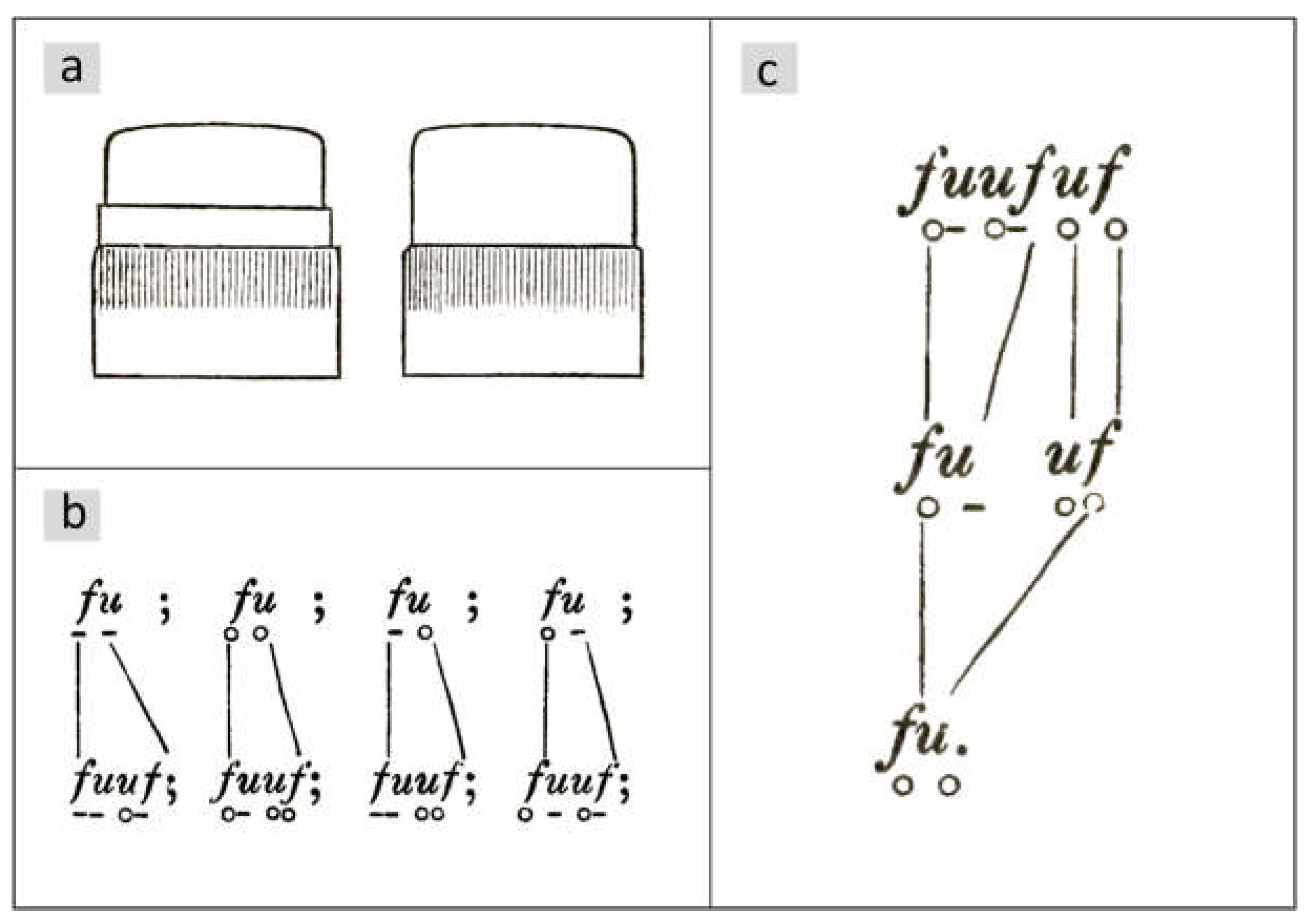
Figure 2.
Colony of Ellerbeckia arenaria according to Otto Müller [10]. The black horizontal lines indicate the valve sizes.
Figure 2.
Colony of Ellerbeckia arenaria according to Otto Müller [10]. The black horizontal lines indicate the valve sizes.
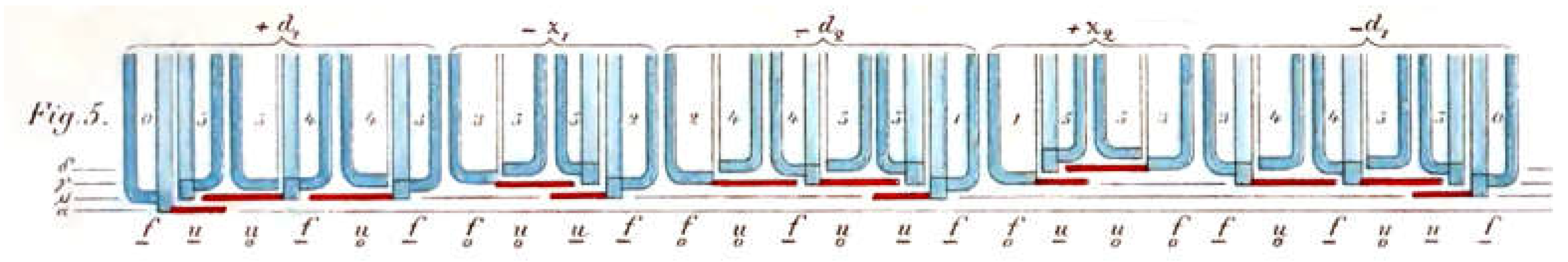
Figure 3.
Sequence of generations according to the model of O. Müller. It is striking that each generation is the beginning of the next.
Figure 3.
Sequence of generations according to the model of O. Müller. It is striking that each generation is the beginning of the next.
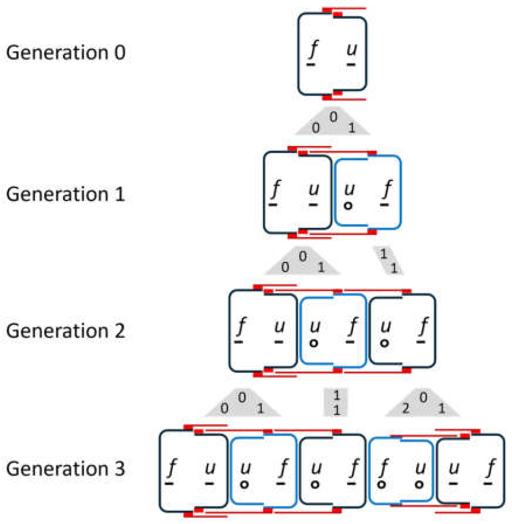
Figure 4.
Four generations are represented by horizontal blue bars. Each generation is formed by copying the previous generation followed by the mirrored and incremented second last generation. This formation is indicated by the grey arrows.
Figure 4.
Four generations are represented by horizontal blue bars. Each generation is formed by copying the previous generation followed by the mirrored and incremented second last generation. This formation is indicated by the grey arrows.
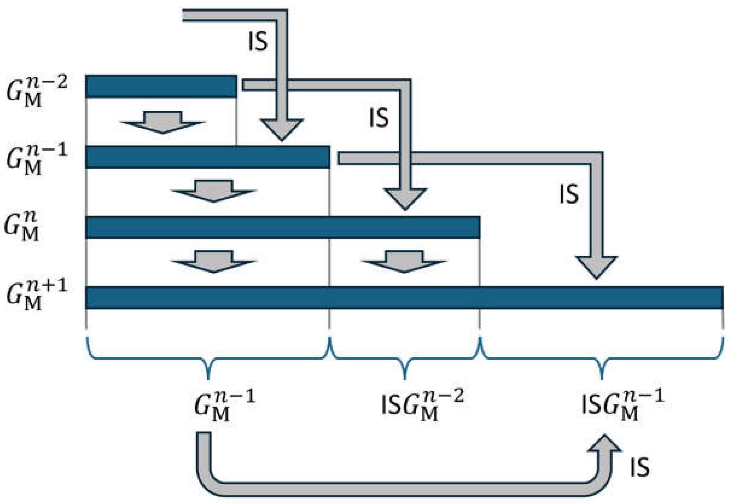
Figure 5.
Visualization of the difference in size indices of the diatoms according to Müller's model. 20 generations were used for the image. The curve starts at the top left, where the color changes are close together.
Figure 5.
Visualization of the difference in size indices of the diatoms according to Müller's model. 20 generations were used for the image. The curve starts at the top left, where the color changes are close together.
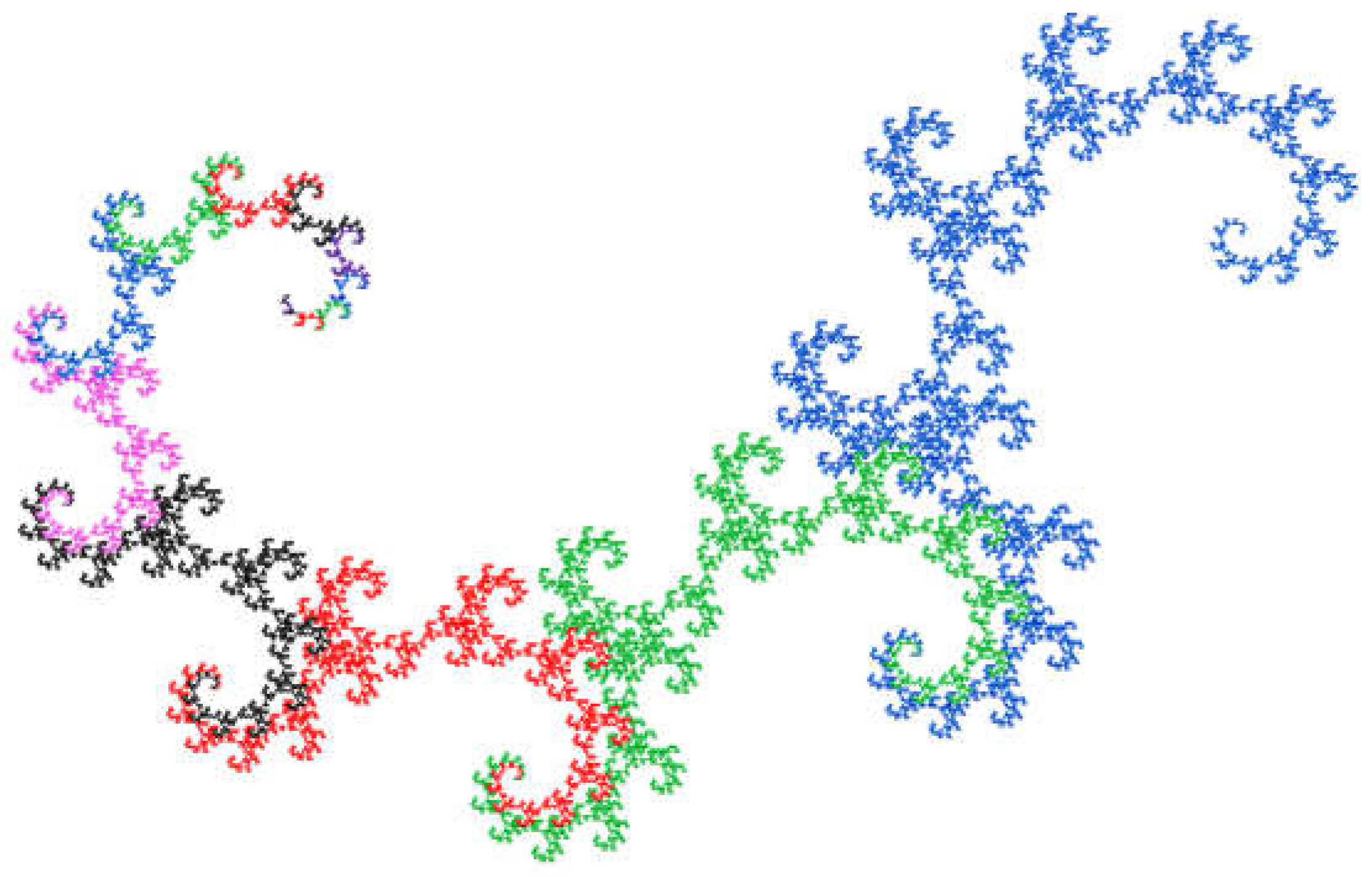
Figure 6.
To obtain a well-structured graphic, the bars representing generations have been right aligned. No part of a previous generation is copied unchanged. This results in a sequence that is not continuously extended.
Figure 6.
To obtain a well-structured graphic, the bars representing generations have been right aligned. No part of a previous generation is copied unchanged. This results in a sequence that is not continuously extended.
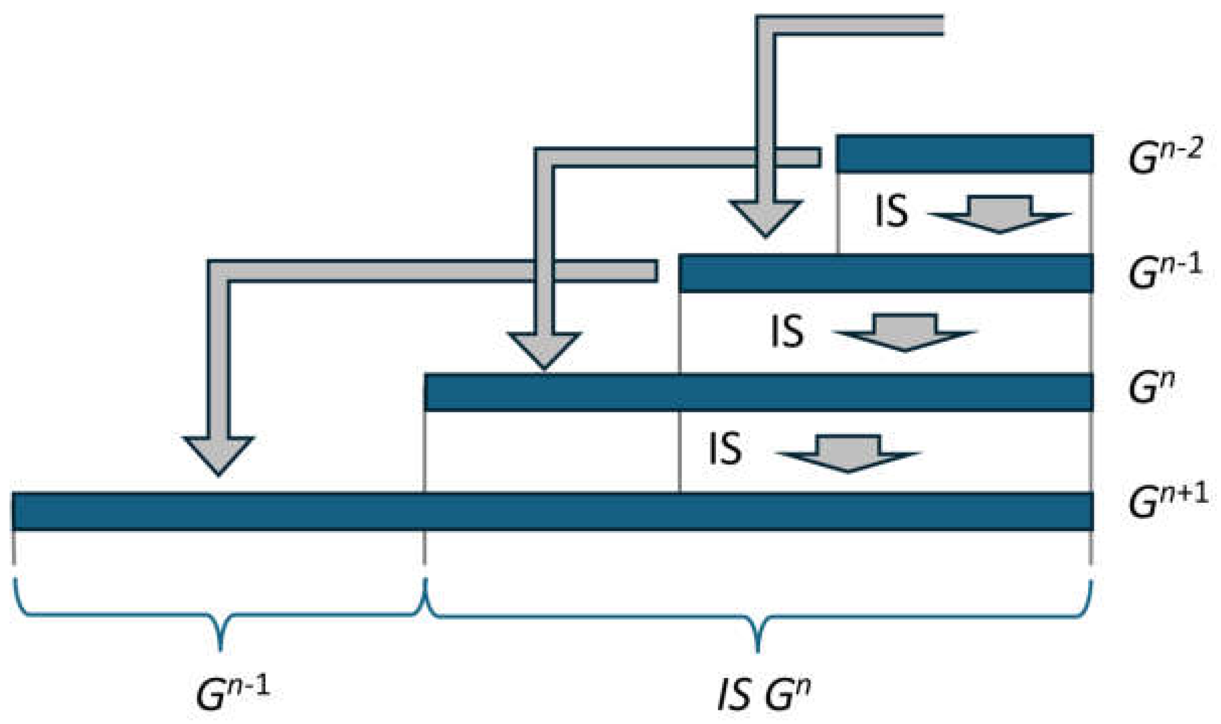
Figure 7.
Visualization of the difference in size indices of the diatoms according to the L-model. 20 generations were used for the image. The curve starts at the top left, where the color changes are close together.
Figure 7.
Visualization of the difference in size indices of the diatoms according to the L-model. 20 generations were used for the image. The curve starts at the top left, where the color changes are close together.
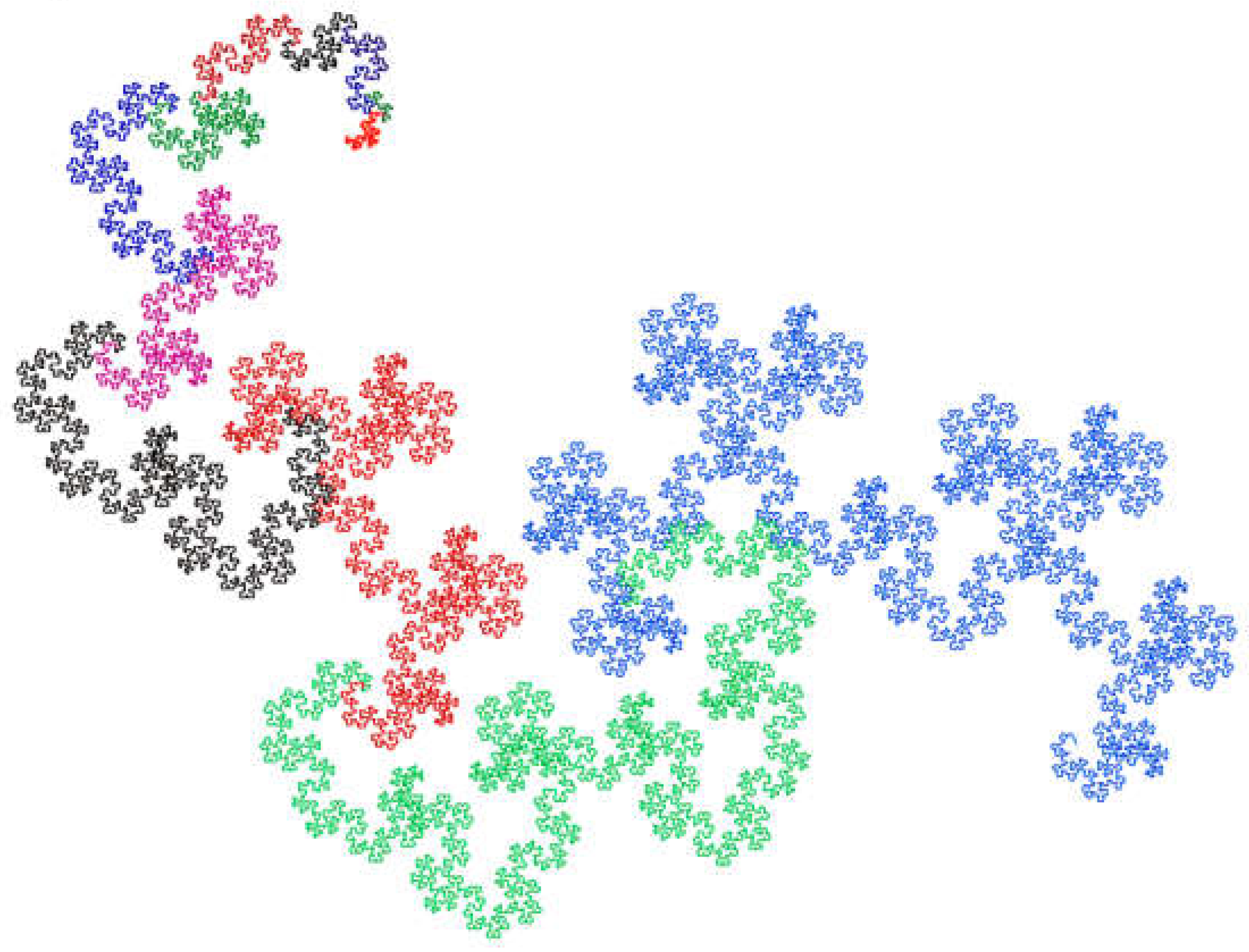
Figure 8.
The number of diatoms with size index k is shown for the models discussed. The number is generally denoted as . (a) Number of diatoms at for the M-model and for the L-model. (b) Decadic logarithm for and values for all three models. (c) Number of diatoms for in the M-model and L-model. (d) Decadic logarithm for and values for all three models.
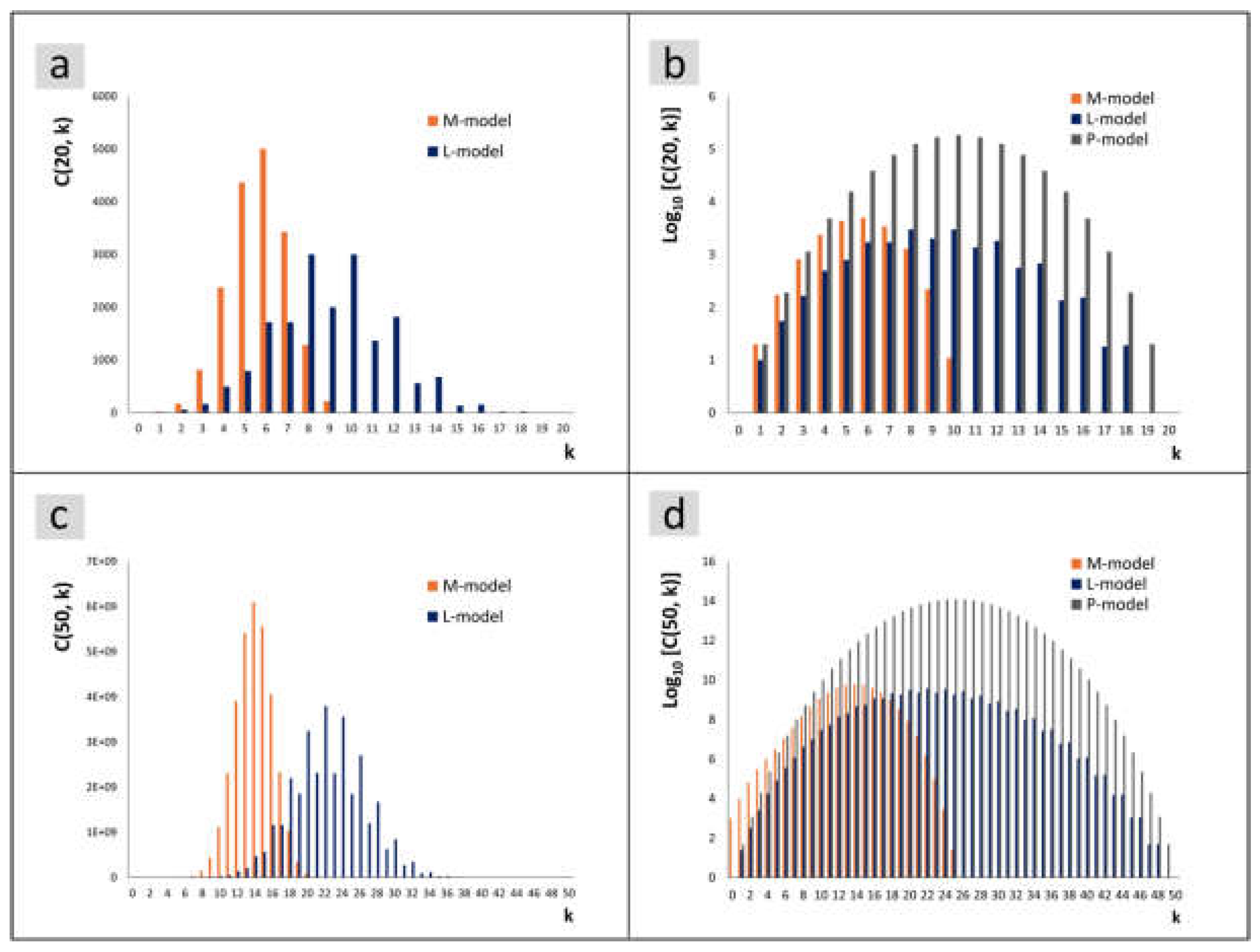

Table 1.
Assignment of the letters of the alphabet to the structure according to Müller [9] with extensions with respect to size index and division behavior.
Table 1.
Assignment of the letters of the alphabet to the structure according to Müller [9] with extensions with respect to size index and division behavior.
| Structure | Diatoms immediately able to divide | Diatoms in an interim state |
|---|---|---|
Disclaimer/Publisher’s Note: The statements, opinions and data contained in all publications are solely those of the individual author(s) and contributor(s) and not of MDPI and/or the editor(s). MDPI and/or the editor(s) disclaim responsibility for any injury to people or property resulting from any ideas, methods, instructions or products referred to in the content. |
© 2025 by the authors. Licensee MDPI, Basel, Switzerland. This article is an open access article distributed under the terms and conditions of the Creative Commons Attribution (CC BY) license (http://creativecommons.org/licenses/by/4.0/).
Copyright: This open access article is published under a Creative Commons CC BY 4.0 license, which permit the free download, distribution, and reuse, provided that the author and preprint are cited in any reuse.


