Submitted:
23 April 2025
Posted:
23 April 2025
You are already at the latest version
Abstract
Mammalian fertilization depends on sperm successfully navigating a spatially and chemically complex microenvironment in the female reproductive tract. This process is often conceptualized as a competitive race, but is better understood as a collective random search. Sperm within an ejaculate exhibit a diverse distribution of motility patterns, with some moving in relatively straight lines and others following tightly turning trajectories. Here, we present a two-state random walk model in which sperm switch from high-persistence-length to low-persistence-length motility modes. We study a circularly symmetric setup with sperm emerging at the center and searching a finite-area disk. We explore the implications of the switching on search efficiency. The first proposed model describes an adaptive search strategy in which sperm achieve improved spatial coverage without cell-to-cell or environment-to-cell communication. The second model that we study adds a small environment-to-cell communication. The models resemble macroscopic search-and-rescue tactics, but without organization or networked communication. Our findings provide a quantitative framework linking sperm motility patterns to efficient search strategies, offering insights into sperm physiology and stochastic search dynamics of self-propelled particles.
Keywords:
sperm cell motion
; search trajectories
; persistence length
Introductory Note:
This paper is in honor of Peter McClintock on the occasion of his 85th birthday. Peter keeps defying stereotypes. For the longest time I thought of him as prototypically British. But then it turned out he was born in Ireland. And given the vigor with which he still hikes, I thought he was in his mid 70s. But then I was recently invited to contribute to an issue of Entropy in honor of his 85th birthday.
I first got to know Peter in the mid 90s. At the time Peter’s work in recognizing the counterintuitive effects that noise can have was groundbreaking. On another front, biophysics was just starting as a field in these days and Peter was at the front of applying physical thinking to cardiac physiology, ion channels, etc. He was and still is unbelievably prolific. With all these editorships and authorships, I still wonder how he ever finds time to sleep, eat, and hike.
And I just know that he will get to a 1000 publications before he will be 100 years old. - Martin Bier
1. Introduction
Mammalian reproduction depends on the ability of sperm cells to locate an egg within the complex microenvironment of the female reproductive tract. Reproductive tracts impose numerous barriers to sperm success, ultimately reducing millions of potential fertilizers to only a few dozen cells that manage to find their way to the ampulla of the oviduct where fertilization takes place. Though rudimentary forms of navigation such as chemotaxis and rheotaxis have been investigated in mammals [1,2], the physiological relevance of these phenomena remains unclear, and may be more significant for externally fertilizing organisms that navigate in three dimensions [3,4]. For nearly all eukaryotes, the sperm search for an egg depends, at least in part, on intrinsically controlled motility patterns. Additionally, among species for which forms of taxis have been shown to be important, it is likely that sperm find themselves in regions or conditions where external guidance cues may be weak or absent - highlighting the importance of understanding how intrinsically controlled motility contributes to the search process.
Though intracellular biochemical mechanisms that control sperm post-ejaculatory behaviors are well-studied in rodents and humans [5], the stochasticity of sperm search owing to complex variation in intrinsically controlled motility patterns remains poorly understood - particularly at the scale of sperm cell populations which vary from to cells per ejaculate depending on the species.
Sperm cells are microswimmers that are subject to the physical limitations of life at low Reynolds number [6], i.e., inertia plays no role and the motion is overdamped. Mammalian sperm, furthermore, move on the epithelial surface of the reproductive tract and 2-dimensional modeling is a reasonable simplification [7]. Sperm motility is driven by active flagellar beating and can be modeled as a random walk [8]. Contemporary computer-aided sperm motility analysis generally focuses on averaged motility patterns on timescales of just a few seconds [9].
A human sperm cell has a width of about 2 m. Human oviducts are called “fallopian tubes.” Fertilization generally occurs in the lining of a fallopian tube. After release in the vagina, only a fraction of less than one-thousandth of the about hundred million sperm cells in a human ejaculate reaches the fallopian tubes. The lining of the fallopian tubes has folds, but can still roughly be thought of as the inside of a cylinder. The cylinder is 10 to 14 cm long and about 1 cm in diameter. The egg cell is an ovoid with a diameter of about 0.15 mm. In other words, we are looking at something the size of a pea that is looking for a big beach ball in a search area that is the size of ten football fields.
An important parameter in this study is the persistence length. The persistence length characterizes the sperm’s trajectory and it can only be observed when the trajectory is followed on a timescale longer than just a few seconds. Persistence length is the distance of over which a curve remains directionally correlated and the concept is also frequently applied in the study of polymers [10,11,12]. We will present the formal definition of persistence length in Section 2. Suffice it to say at this point that a trajectory with a long persistence length appears as a relatively straight path. A smaller persistence length, on the other hand corresponds to more frequent changes in direction. Sperm within one ejaculate can exhibit persistence lengths that may differ by orders of magnitude (cf. Figure 1).
Recently, transitions between high-persistence-length movement and low-persistence length movement have been observed in bovine sperm [13]. This suggests that sperm may transition between mere dispersal and localized search behavior. In confined or semi-confined domains, such as an oviduct in-vivo or a culture dish surface in-vitro, effective sperm navigation likely requires a strategy that balances rapid traversal across searchable surface area with thorough exploration of local space [8]. The efficiency of sperm search may depend on transition rates among movement patterns. Transitions between different movement patterns have also been observed in E. coli bacteria [14]. In that case the transitions between the “movement states” were well-described with ordinary chemical kinetics (i.e., exponentially distributed dwelling times in states).
Here, we hypothesize that this two-state random walk — switching from a high-persistence length to a low-persistence length, can enhance search efficiency in domains where uniform coverage is essential. We develop a two-state active particle model to explore this hypothesis on a disk with an absorbing boundary where we let searchers emerge from the center of the disk. In Section 2, we show through numerical simulation how changes in persistence length can improve coverage of the search domain. As a baseline, we examine the case of a searcher with a constant persistence length. Next we study two enhancements. The first one involves a well-tuned transition rate (i.e. exponentially distributed waiting times) to a persistence length that is about an order of magnitude smaller. There is evidence that the change-of-state can be catalyzed by chemicals that are present in the environment [13,14]. Taking into account this positional guidance, we also study, as a second case, a modified version of our first model: we take the stochasticity out of the switch and let the searching sperm cell change its motility state upon entering the outer section of the disk. In Section 3, we use the diffusion equation to add mathematical rigor to results of Section 2.
2. A Two-State Random Searcher on a Disk
Our geometric setup is simple. Searching particles appear in the center of a disk and follow a random trajectory until they hit the absorbing boundary at the circumference. We set the disk’s radius at (cf. Figure 2). Each moving searcher starts out with a large persistence length that is on the order of magnitude of the radius of the disk. The switch is to a persistence length that is about an order of magnitude smaller. We gather statistics for three cases. (i) A persistence length that is fixed at half the disk’s radius and does not change. (ii) A persistence length that is initially set at one-and-a-half times the disk’s radius, but with a transition rate that is set such that the irreversible switch to the smaller persistence length occurs on average at about . (iii) Persistence lengths as in the 2nd case, but with the irreversible switch occurring at the moment that is first crossed. We consider a search effective if there is no place for the target to “hide” on the disk. In practical terms this means that all parts of the disk are equally searched. We divide the disk into annuli and numerically investigate. In the next section we will also set up and analyze a diffusion equation to help us understand the results of the stochastic simulations.
We model the sperm cell as an active particle that moves at a constant speed . Fluctuations in the direction of motion are accounted for with a diffusion coefficient . This stochasticity is due to active flagellar fluctuations, rather than Brownian motion [15]. We let be the unit vector in the direction of motion and come to the following equations describing the sperm cell’s motion:
At any time the unit vector in the direction of motion is given by . The term represents Gaussian-distributed white noise. We use the Euler-Maruyama scheme for the actual numerical simulations: at every timestep the angle is updated through the addition of a small random number. The actual is implemented by taking a set of Gaussian distributed numbers that are zero-average and unit variance. Subsequent values of are obtained by dividing these numbers by the square root of the timestep .
The trajectories generated by Equation (1) display a persistence length . Persistence length is a notion that is also well known in polymer theory [10,11,12]. We parametrize the trajectory with the contour length ℓ. Obviously, the direction changes as a function of ℓ. We consider the orientations and , i.e., the orientations on two points that are a distance ℓ away from each other along the contour. A good measure for the correlation between and is the average , where and the average is taken over all positions along the entire trajectory such that the different segments of length ℓ do not overlap. For a very stiff almost straight trajectory, is close to one for all ℓ. The persistence length is defined through [10,11,12]. A smaller persistence length makes a trajectory appear more tightly wound (cf. Figure 2).
Related to the persistence length is the Kuhn length. Imagine a point P along the trajectory. Points that are to the left and right of P come with orientations that are not correlated to the orientation at P. With this realization we can next imagine the trajectory as being built up from straight segments with a length of . At each junction, the angle between the linked segments is a random number from a flat distribution between 0 and . The polymer or trajectory conceived as such is called a Freely Jointed Chain (FJC) and is known as the Kuhn length.
The FJC comes with concise formulae. For a chain of a total length L and with N Kuhn segments of length , we have
for the total contour length and the average square end-to-end distance, respectively. These formulae are well-known, much applied, and explained in many authoritative textbooks, though mostly in the context of polymer theory [10,11,12].
For a searching particle that emerges at the center of the disk, it makes sense to search in such a way that any random point on the disk has an equal likelihood of being “found.” An annulus at a distance r from the center of width covers an area (cf. Figure 2). A search by a moving particle is thus more likely to be successful if the dwelling time at radius r is proportional to r itself. For an effective search, the trajectory should get tighter as the rim is approached, i.e., the Kuhn length should decrease during the search. A simple physiological course of action to achieve such decrease of is to emerge from the center with an initial Kuhn length and a well-tuned transition rate to a smaller value .
Consider the disk with radius as depicted in Figure 2. Figure 2a shows a search with and , which implies a persistence length of . Figure 2b depicts the realization of a search with an initial and a transition rate to a final . Note that the of Figure 2a is the geometric average of and .
The unit disk has three times as much area outside as that it has inside . It thus makes sense to explore the disk’s outer part () with three times the contour length of the inner part. After some algebra, it follows from Equation (2) that with a Kuhn length that is one-ninth of the original one, approximately the same end-to-end distance is covered with three times the contour length. It is therefore that we take . Finally, it needs to be noted that for all generated trajectories we took for the timestep.
In Figure 2 the unit disk is divided up into nineteen annuli each with a width of 1/20. In the center there is one small circle with radius 1/20. A search is most effective if each location on the disk has an equal chance of being visited by the searcher. In terms of the annuli this means that in each annulus, the searching particle spends the same amount of time per unit of area, i.e., (cf. Figure 3) should be constant. Each of the three bar charts in Figure 3 is the result of 5000 trajectories that were generated with Equation (1). For each trajectory the amount of time in each annulus was recorded and then divided by the area of that annulus. Figure 3 represents the average over 5000 trajectories for three cases. For Figure 3a the radial diffusion coefficient was held constant at . For Figure 3b each of the 5000 searchers starts at the origin with and a transition rate to . Figure 3c depicts the result for searchers that can detect their own position and irreversibly switch from to when is first traversed.
Going from Figure 3a to Figure 3b we see an improved search. The average and standard deviation of over the twenty regions go from 1.1 and 1.5 to 1.7 and 1.7, which implies that the coefficient of variation (the standard deviation divided by the average) goes from 1.3 to 0.98. Furthermore, the escape time , i.e. the average time it takes to go from the center of the disk to , increases from to in the setup with the switch of .
There is another small improvement as we go from Figure 3b to Figure 3c, i.e. go to a setup where the searcher “reads” its position and makes the switch contingent on the position. For the search in Figure 2c, the average and standard deviation are 1.6 and 1.5, resulting in a coefficient of variation of 0.94. The value of is the same as for the non-position guided switch, i.e., . Particularly striking in Figure 3c is how stays constant in the region between about and .
The improvements going from Figure 3a to Figure 3b and next to Figure 3c may appear small. However, in the 1930s the “New Evolutionary Synthesis” combined genetics and population dynamics to put evolution on a more quantitative and scientifically rigorous foundation. It was found that even small selective advantages drive evolution. The authoritative textbook by D. Futuyma [16] summarizes it as follows: “. . . a character state with even a miniscule advantage will be fixed by natural selection. Hence even very slight differences among species, in seemingly trivial characters such as the distribution of hairs on a fly or veins on a leaf, could conceivably have evolved as adaptations.”
3. The Evolution of the Probability Distribution on the Disk
The previous section involved an ordinary differential equation with a stochastic input at every timestep. The ensuing stochastic differential equation describes a trajectory of the diffusing particle. It is possible to formulate an equivalent partial differential equation that describes the time evolution of the particle’s probability distribution . The underlying theory is covered in many standard textbooks [17,18,19].
The equation that rules the 2D diffusion on the disk is
Here D and stand for the diffusion coefficient and the Laplace operator, respectively. The diffusion coefficient D in this equation has a simple relation to the in Equation (1). For a particle diffusing in 2D, the mean square displacement and the elapsed time are related through . The can be identified with S in Equation (2). The contour length L can be identified with . This leads first to and, after invoking and , we find
In polar coordinates and with circular symmetry, Equation (3) takes the form
Before further analysis, it is worth reflecting on Equation (5) in the light of what was established in the previous section. The first term on the right-hand-side of Equation (5) is a diffusion term that does not discriminate between the directions r and . The second term on the right-hand-side is a drift term that contains a characteristic speed . This may be puzzling as the diffusion should have no apparent direction. In his classic text, Feller [20] explains the apparent anisotropy as follows (Volume 2, Chapter 10, Section 6): “The existence of a drift away from the origin can be understood if one considers a plane Brownian motion starting at the point r of the x-axis. For reasons of symmetry its abscissa at epoch is equally likely to be or . In the first case certainly , but this relation can occur also in the second case. Thus the relation has probability , and on the average R is bound to increase.”
With an initial condition and on a disk with infinite radius, Equation (5) is readily solved by the spreading Gaussian:
This solution comes with a root-mean-square distance to the origin, , that increases following . Taking the derivative w.r.t. time on both sides, we find for the speed of the root-mean-square distance .
For a particle that drifts away from the origin with a speed , the time that is spent in an annulus of area , is found to be . So the search time per area, , appears to be independent of r. This uniform coverage of the search area occurs with any drift speed that is proportional to .
However, it is not hard to see that such r-independence of only works for a disk with a radius . If a diffusing particle is absorbed upon hitting the boundary at a finite , any trajectory leading to a position after passing through an region is eliminated. This leads to a decreasing as r increases. Such decrease is indeed what we see in Figure 3. Below we will add mathematical rigor to these insights and observations.
An absorbing boundary at means . Solutions for setups with an absorbing boundary condition can commonly be found through placing an “image initial condition,” , outside the disk. The image is negative and the positioning of the image initial conditions has to be such that the ensuing flow towards (governed also by Equation (5)) leads to . The full solution then satisfies Equation (5) in the area .
For 1D diffusion along an axis, the image method is easily implemented and readily leads to a solution. But complications arise in the 2D case. As was mentioned before in the context of Equation (5), the directions towards the disk’s center and away from the disk’s center are not equivalent. For an image that is initially positioned at , i.e. , a solution according to Equation (5) can be derived after some nontrivial mathematical operations [21]: , where represents the Modified Bessel function of the first kind. The problem with this solution is that we do not have at all times.
Below we derive some relevant features of the diffusion on the 2D disk without an actual closed-form solution. Through Fick’s Law, the outflow from the disk can be identified with . If we set for the slope of the curve at (cf. Figure 4), then we have at . is also a good approximation on near the outer edge of the disk.
In our 2D case, the flux is the amount of probability that crosses at per unit of time and per unit of distance along the circumference of the circle with radius . Next it is the ratio that represents the average speed that is necessary to bring about this flux. With , we then obtain for the drift speed of the diffusing particle. We observe that, unlike with the case discussed earlier, the drift speed now goes up as the absorbing boundary of the disk gets closer. This can be readily intuited upon the realization that with more nearby, ever more possible trajectories hit and disappear from the domain.
As before, we divide up our disk in annuli of a width . With the drift speed that we derived in the last paragraph, we find for the dwelling time per annulus . From there we derive a search time per area that depends on r:
It is obvious that vanishes as . Figure 5 shows the results of a simulation. We let 1000 particles diffuse from the center of the disk to the absorbing boundary at . The motion of the particles is again ruled by Equation (1) with and . Through Equation (4) this leads to . The timestep used for the Euler scheme was again . As before, the unit disk was segmented into a small disk and nineteen annuli of a width of 0.05. Like before, the twenty bars in the histogram (Figure 5a) give the average time per unit area spent in each of the twenty segments. Figure 5b gives for the four outermost annuli together with the best fitting straight line. Equation (7) gives 63.7 for this slope. The slope of the fitted line is 67.7. The small discrepancy is not just due to the neglected curvature, but also to the finite persistence length that is implicit in simulating Equation (1). In our case . The partial differential equations that are central in this section, i.e., Equations (3) and (5), actually correspond to a fractal trajectory with a zero persistence length.
A diffusion coefficient that decreases as the particle diffuses away from the center leads to a D that effectively decreases with r. As was pointed out in the previous section and as now also should be clear from Equation (7), this flattens out as a function of r and leads to a more efficient search of the disk’s area.
Finally, it is worth pointing out that Equation (7) and the drift speed are independent of the actual slope . This is a nice feature, because as the particle diffuses away from , that slope actually changes over time. Immediately after , the slope increases. Later in the relaxation, the slope starts decreasing again. It is remarkable that Equation (7) and the drift speed remain the same throughout that process.
4. Discussion
We have studied a simple, bare-bone model to keep the analysis intuitive and to have manageable mathematics and numerics. Figure 6 presents a model with more realism. In the oviduct the searching sperm cells enter on one side. Here we have them enter at an arbitrary point on the left edge. We account for being on the inside of a cylinder through a periodicity of the vertical coordinate. The two-state strategy that we studied on the disk would also likely be effective in this case. A good dispersal of searchers could be achieved by taking off with a large persistence length in an arbitrary direction from an arbitrary point on the left edge. Each individual sperm cell would next do its more detailed search after it switches to the smaller persistence length.
Some of the trajectories in Figure 1 exhibit chirality. In our minimal model we did not not consider chirality. The chirality could readily be added to the model in Equation (1) through the addition of an angular velocity on the right-hand-side of the second equation. Such study was undertaken in Ref. [13]. It is obvious that chirality, or any curvature for that matter, is like a smaller Kuhn length in that it leads to an area being more thoroughly searched.
Routine semen analysis in clinical practice relies on microscopic inspection of sperm characteristics and statistical comparison with fertile samples [22,23]. Contrary to what is commonly thought, fast motility alone is not necessarily an indicator of high fertilizing potential due to the complexity of the sperm search task and statistical variation among the large number of sperm present in an ejaculate [24]. Efficient search likely requires a combination of motility patterns including high-persistence-length movement for rapid dispersal, and low-persistence-length movement for thorough local exploration. Our modeling suggests that a well-tuned combination of both modes may enhance search efficiency on restricted domains such as those that occur in the complex environment of the female reproductive tract, where sperm must balance wide-area coverage with detailed exploration to locate the egg.
The two-state random walkers (Figure 2b and Figure 3b,c) that we studied represent improvements over the regular random walk (Figure 2a and Figure 3a). In closing, it is instructive to look at our subject matter and results from the wider perspective of computation and problem solving in biological systems. Searches are also part of macroscopic everyday reality. When a search-and-rescue team goes looking for a lost or missing person in a large wilderness area, a common strategy is to cut up the search area. The smaller areas get labeled and next different teams or individuals are assigned to different areas in the grid for detailed searches. Obviously, sperm cells cannot achieve such a level of organization and coordination.
The random walk with identical searchers with constant persistence length (cf. Figure 2a) is the most brute-force approach to the search problem. It is the Monte-Carlo modus operandi and it requires the mobilization of many searchers to achieve a nonegligible probability of fertilization. The random walk of Figure 2b and Figure 3b contains a transition to a smaller persistence length. We have shown that this feature leads to improved efficacy. Through the transition rate k, this search involves a characteristic time . So the improvement is due to the usage of a very crude clock and the search being split up into a “before” and “after.” Figure 3c is the barchart that corresponds to a random-walk searcher that does not have a clock, but instead uses a very crude GPS. The searcher only “knows” whether it is in Region 1 or 2, and switches persistence length the first time it “sets foot” in Region 2.
Biologically, a well-tuned k or an effective partitioning into two regions would be an outcome of natural selection. This improvement over the pure Monte-Carlo algorithm can be viewed as enhanced agency and as something “learned” - a genetic legacy built up after much past “trial and error.” Neither of the two improvements involve any sperm-to-sperm communication.
The analogy with a team on a search-and-rescue mission underscores an important point. Popular culture often views ejaculate as a swimming contest. However, it is more appropriate to see ejaculate as tissue. A heart pumps, an ear to detect sound, and ejaculate searches. Successful ejaculate is ejaculate that yields a high probability that one sperm cell finds and fertilizes an egg cell. It is obvious that there is selectional pressure towards more successful ejaculate.
Author Contributions
Conceptualization, M.B., M.M., and C.S.; methodology, M.B., M.M., and C.S.; software, M.B.; formal analysis, M.B. and M.M.; investigation, M.B., M.M., and C.S.; writing—original draft preparation, M.B.; writing—review and editing, M.B., M.M. and C.S.; supervision, C.S. All authors have read and agreed to the published version of the manuscript.
Funding
This work was supported by the Eunice Kennedy Shriver National Institute of Child Health and Human Development (R01HD110170 to CAS), as well as laboratory startup funding from the Thomas Harriot College of Arts and Sciences at East Carolina University and the East Carolina University Research and Economic Development Office (CAS). M.M. gratefully acknowledges financial support for this project by the Fulbright Scholar-In-Residence Program, sponsored by the U.S. Department of State.
Acknowledgments
We are grateful to Łukasz Kuśmierz and David Hart for useful feedback.
Conflicts of Interest
The authors declare no conflict of interest.
References
- Miki, K.; Clapham, D.E. Rheotaxis guides mammalian sperm. Curr. Biol. 2013, 23(6), 443–452. [Google Scholar] [CrossRef] [PubMed]
- Eisenbach, M. Mammalian sperm chemotaxis and its association with capacitation. Dev. Genet. 1999, 25, 87–94. [Google Scholar] [CrossRef]
- Kromer, J. A.; Märcker, S.; Lange, S.; Baier, C.; Friedrich, B.M. Decision making improves sperm chemotaxis in the presence of noise. PLOS Comput. Biol. 2018, 14. [Google Scholar] [CrossRef] [PubMed]
- Domb, C. On multiple returns in the random-walk problem. Math. Proc. Cambridge Philos. Soc. 1954, 50, 586–591. [Google Scholar] [CrossRef]
- Gervasi, M.G.; Visconti, P.E. Chang’s meaning of capacitation: A molecular perspective. Mol. Reprod. Dev. 2016, 83, 860–874. [Google Scholar] [CrossRef] [PubMed]
- Purcell, E.M. Life at low Reynolds number. Am. J. Phys. 1977, 45, 3–11. [Google Scholar] [CrossRef]
- Woolley, D.M. Motility of spermatozoa at surfaces. Reproduction 2003, 126, 259–270. [Google Scholar] [CrossRef] [PubMed]
- Brisard, B.M.; Cashwell, K.D.; Stewart, S.M.; Harrison, L.M.; Charles, A.C.; Dennis, C.V.; Henslee, I.R.; Carrow, E.L.; Belcher, H.A.; Bhowmick, D.; Vos, P.W.; Majka, M.; Bier, M.; Hart, D.M.; Schmidt, C.A. Modeling diffusive search by non-adaptive sperm: empirical and computational insights. PLOS Comput. Biol. 2025, 21. [Google Scholar] [CrossRef] [PubMed]
- Hansen, J.N.; Rassmann, S.; Jikeli, J.F.; Wachten, D. SpermQ–a simple analysis software to comprehensively study flagellar beating and sperm steering. Cells 2018, 8, 10. [Google Scholar] [CrossRef] [PubMed]
- Rubinstein, M.; Colby, R.H. Polymer Physics; Oxford University Press: New York, 2003. [Google Scholar]
- Grosberg, Yu.A.; Khokhlov, A.R. Giant Molecules; Academic Press: San Diego, 1997; p69–91. [Google Scholar]
- Boal, D. Mechanics of the Cell; Cambridge University Press: Cambridge, UK, 2002. [Google Scholar]
- Zaferani, M.; Abbaspourrad, A. Biphasic chemokinesis of mammalian sperm. Phys. Rev. Lett. 2023, 130, 248401. [Google Scholar] [CrossRef] [PubMed]
- Perez Ipin˜a, E.; Otte, S.; Pontier-Bres, R.; Czerucka, D.; Peruani, F. Bacteria display optimal transport near surfaces. Nature Physics, 2019, 15, 610–615. [Google Scholar] [CrossRef]
- Ma, R.; Klindt, G.S.; Riedel-Kruse, I.H.; Jülicher, F.; Friedrich, B.M. Active phase and amplitude fluctuations of flagellar beating. Phys. Rev. Lett. 2014, 113, 048101. [Google Scholar] [CrossRef] [PubMed]
- D.J. Futuyma, Evolution; Sinauer Associates: Sunderland, MA, 2005.
- van Kampen, N.G. Stochastic Processes in Physics and Chemistry; Elsevier: Amsterdam, 1992. [Google Scholar]
- Gardiner, C.W. Handbook of Stochastic Methods, 2nd ed.; Springer: Berlin, 1985. [Google Scholar]
- Risken, H. The Fokker–Planck Equation; Springer: Berlin, 1989. [Google Scholar]
- Feller, W. An Introduction to Probability Theory and its Applications, Vol. 2; John Wiley & Sons, Inc.: New York. 1971.
- Hahn, D.W.; Necati Özişik, M. Heat Conduction; John Wiley & Sons, Inc.: Hoboken, NJ, 2012. [Google Scholar]
- Tanga, B.M.; Qamar, A.Y.; Raza, S.; Bang, S.; Fang, X.; Yoon, K.; Cho, J. Semen evaluation: methodological advancements in sperm quality-specific fertility assessment — A review, Anim. Biosci. 2021, 34, 1253–1270. [Google Scholar] [CrossRef] [PubMed]
- Boitrelle, F.; Shah, R.; Saleh, R.; Henkel, R.; Kandil, H.; Chung, E.; Vogiatzi, P.; Zini, A.; Arafa, M.; Agarwal, A. The sixth edition of the WHO manual for human semen analysis: a critical review and SWOT analysis. Life(Basel) 2021, 11, 1368. [Google Scholar] [CrossRef] [PubMed]
- Martínez-Pastor, F. What is the importance of sperm subpopulations? Anim. Reprod. Sci. 2022, 246, 106844. [Google Scholar] [CrossRef] [PubMed]
Figure 1.
Typical trajectories followed by about 20 human sperm cells in the course of 26 seconds in a m square and viewed under a microscope. The sperm cells are observed to move at roughly the same speed, but persistence lengths differ widely.
Figure 1.
Typical trajectories followed by about 20 human sperm cells in the course of 26 seconds in a m square and viewed under a microscope. The sperm cells are observed to move at roughly the same speed, but persistence lengths differ widely.
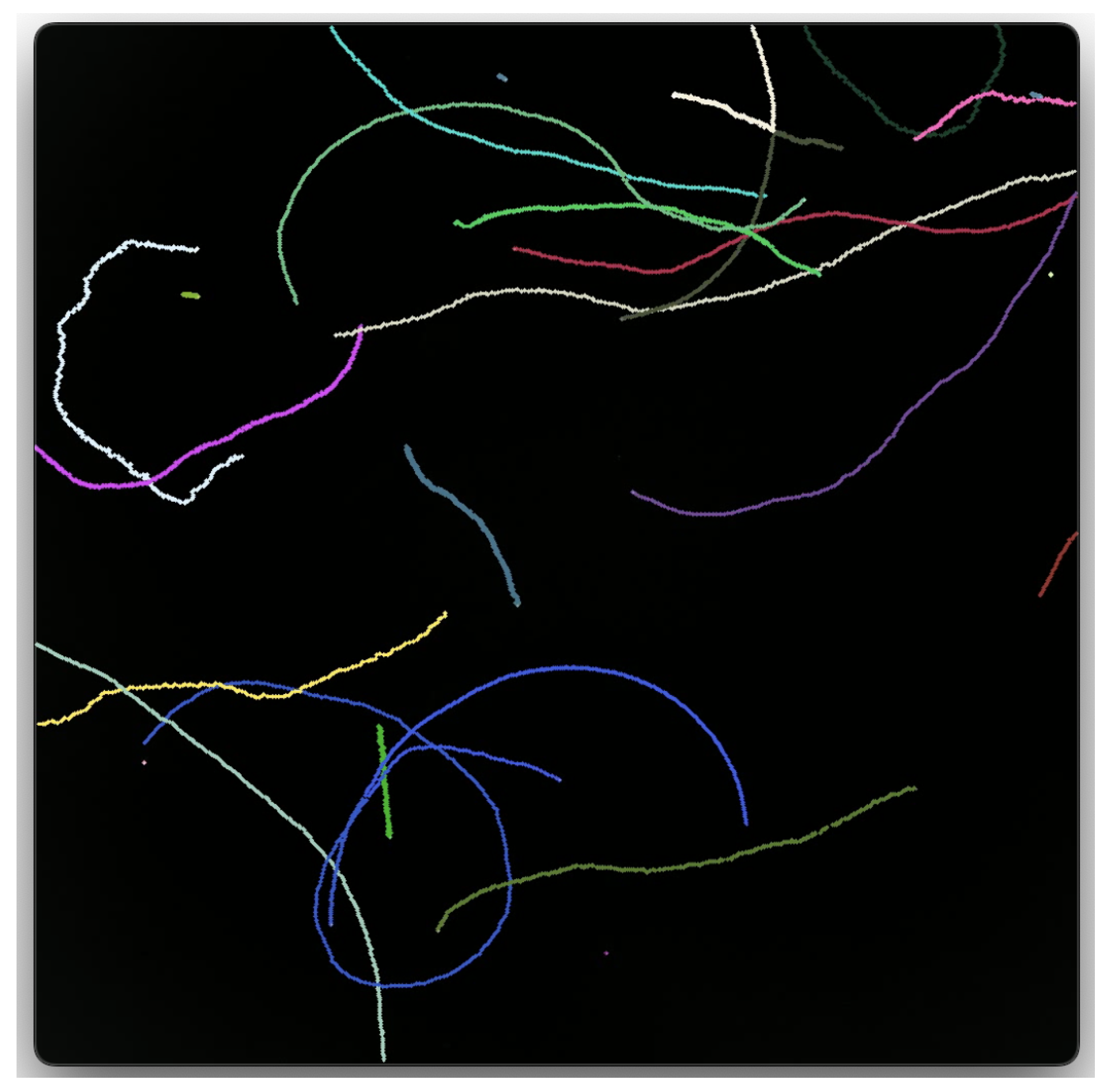
Figure 2.
(a) The searching particle appears in the center of the unit disk and follows Equation (1) with and . The timestep is and the edge of the disk is an absorbing boundary. (b) Initially the angular diffusion coefficient is . There is a transition rate to switch to . The part of the trajectory before the switch is almost ballistic and in red. The remaining part is in blue. With for the transition rate, the switch will on average occur close to . All numerical work in this article was carried out with the Mathematica software package.
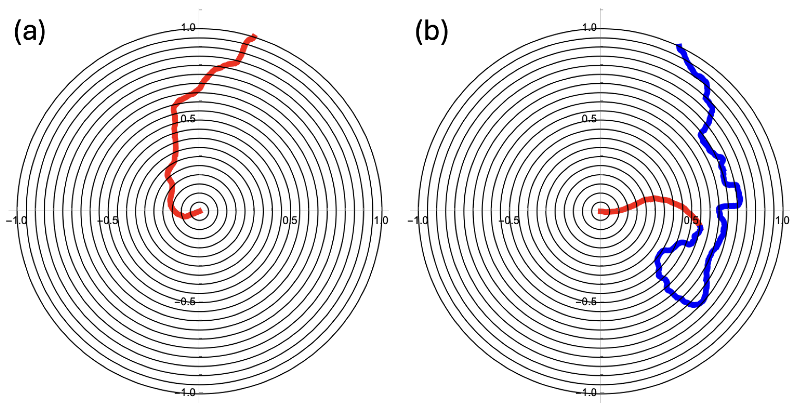
Figure 3.
(a) Trajectories as in Figure 2a were generated and for each region (one small circle and nineteen annuli) the time spent per unit area, , was recorded. Figure 3a depicts the averages over 5000 trajectories. (b) As for Figure 2b, we have implemented a varying : the searcher leaves the origin with a constant transition rate to the larger value of . This leads to an improved search in that becomes larger and more constant. (c) Figure 3c shows how further improvement is achieved upon giving the searcher the ability to “read” its position and let the irreversible transition to the larger occur when is first traversed. Details are in the text.
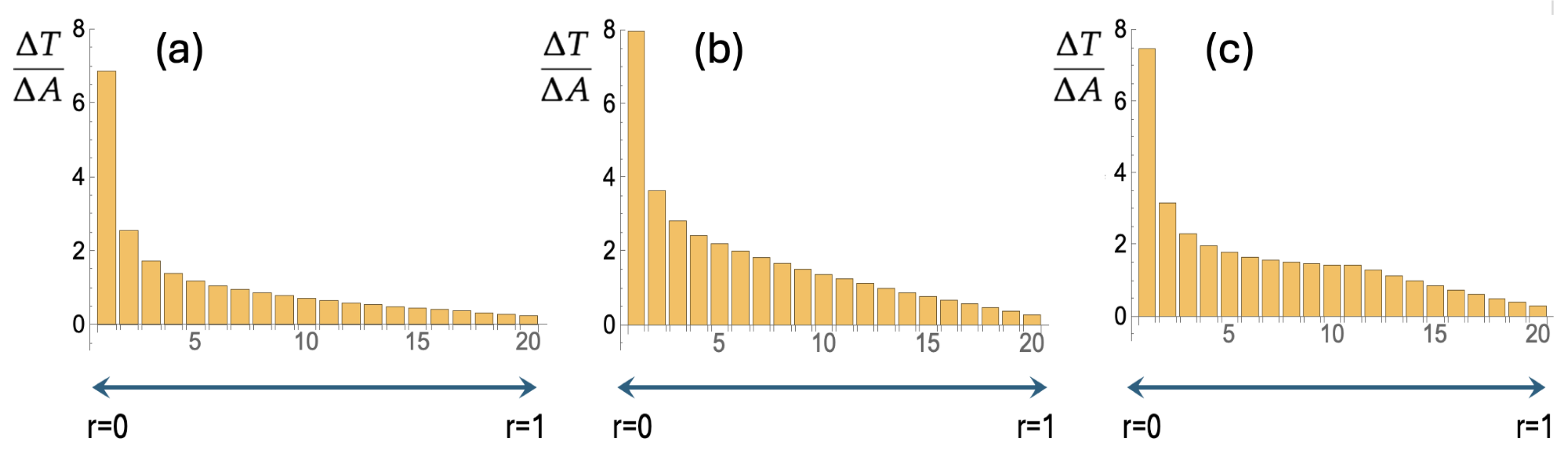
Figure 4.
To our knowledge, Equation (5) has no analytic solution on a disk with an initial condition and an absorbing boundary at a finite . The absorbing boundary implies at all times for the evolving . We have for the slope at . We take this as a first approximation also near the rim. This implies for the amount of probability that crosses the circumference of the disk per unit of time and per unit of distance. With near , we find for the drift speed towards the rim. Note that this result is independent of . The drift speed will thus stay at the same value during the entire relaxation.
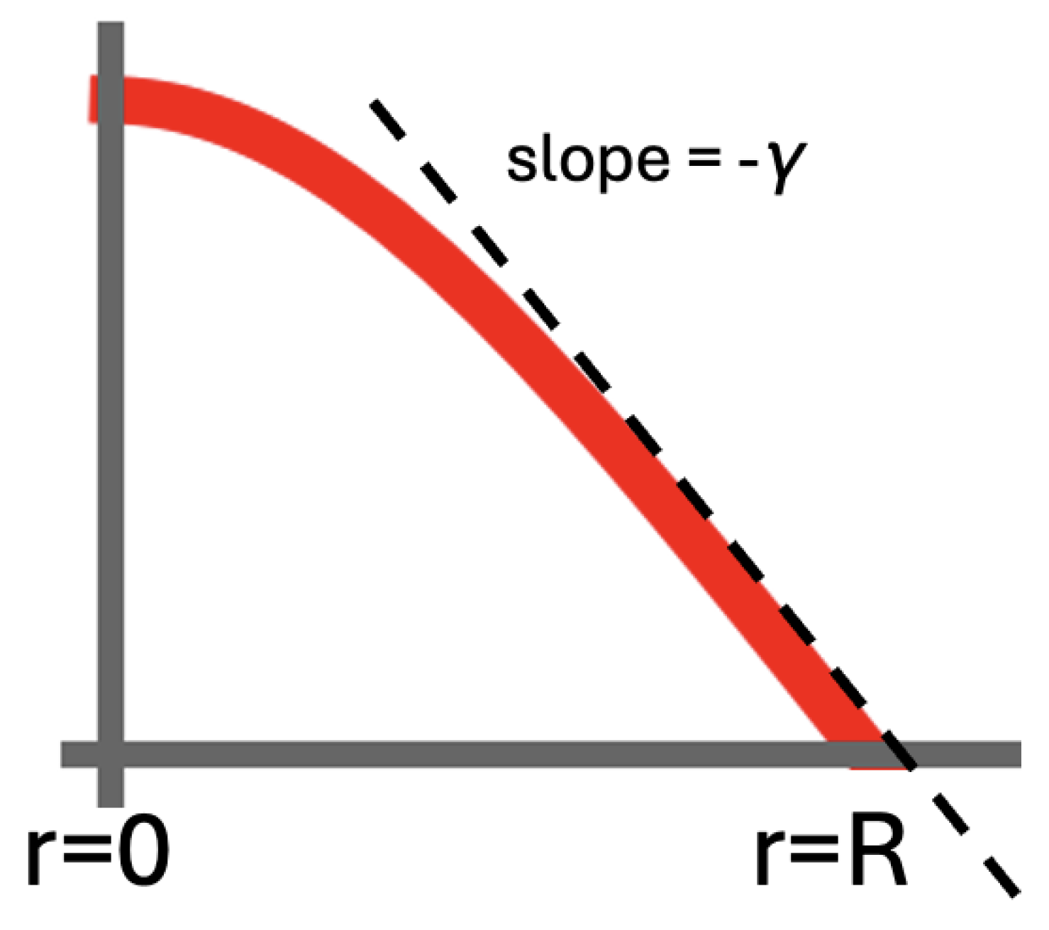
Figure 5.
Equations (3) and (5) are only valid if , i.e., if is very large. We simulate as in Figure 2 and Figure 3, but with leading to . The figure on the left is the ensuing barchart (cf. Figure 3). The figure on the right is a zoom-in on the last four bars of the barchart together with the best linear fit. The slope of the fit is in good agreement with the prediction of Equation (7).
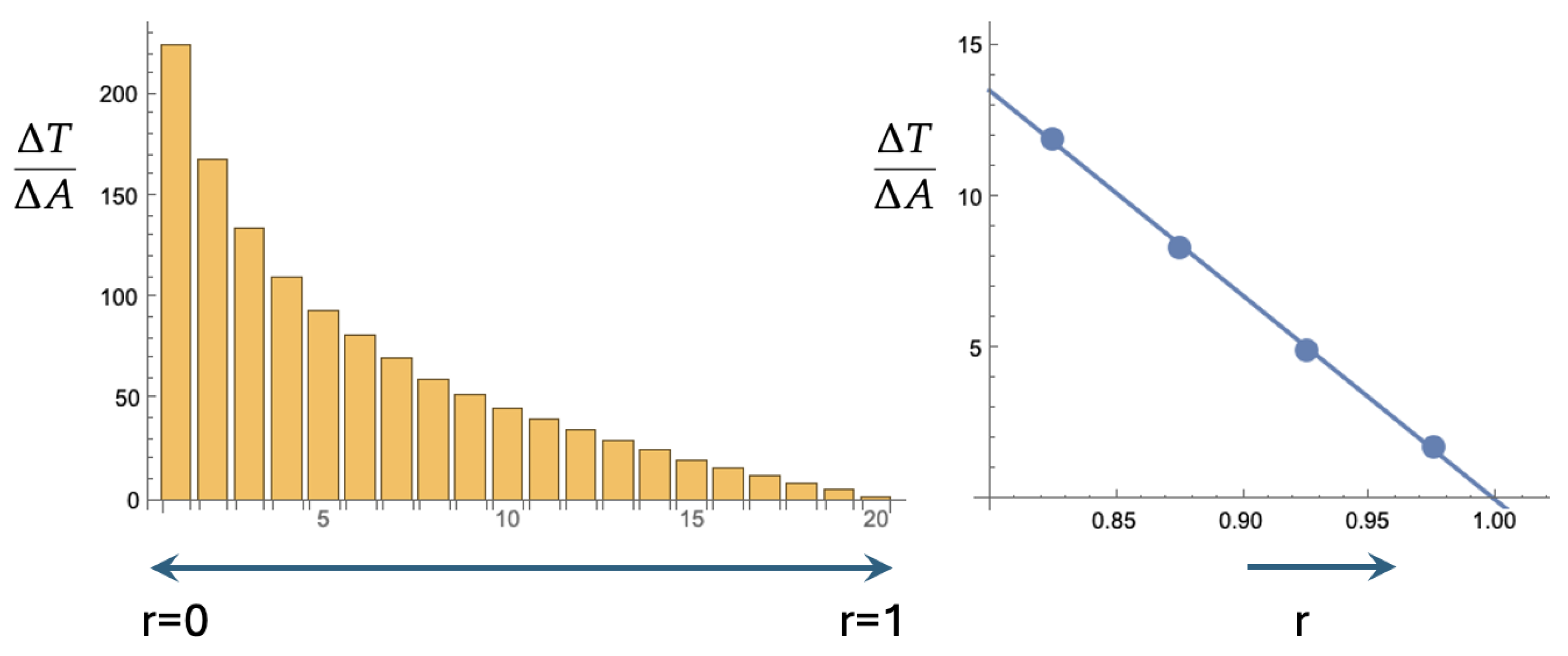
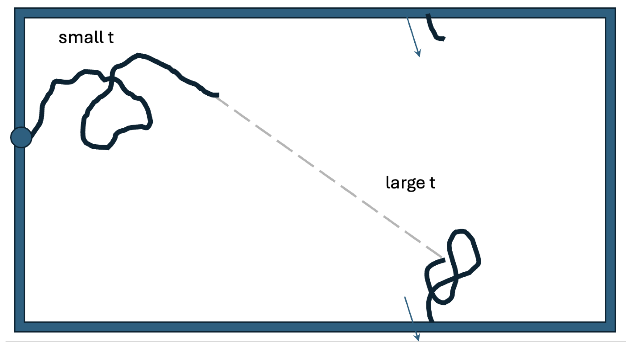
Figure 6.
It is in the cylindrical oviduct that a sperm cell searches for the egg. This search can be modeled as a random walk that starts on the left and has an absorbing boundary on the right. The vertical coordinate is periodic. The geometry is a bit more complicated than this as the oviduct’s surface has many twists and folds. But even so, it makes sense for the searchers to first rapidly disperse and to later switch to a smaller persistence length for a more detailed search.
Disclaimer/Publisher’s Note: The statements, opinions and data contained in all publications are solely those of the individual author(s) and contributor(s) and not of MDPI and/or the editor(s). MDPI and/or the editor(s) disclaim responsibility for any injury to people or property resulting from any ideas, methods, instructions or products referred to in the content. |
© 2025 by the authors. Licensee MDPI, Basel, Switzerland. This article is an open access article distributed under the terms and conditions of the Creative Commons Attribution (CC BY) license (http://creativecommons.org/licenses/by/4.0/).
Copyright: This open access article is published under a Creative Commons CC BY 4.0 license, which permit the free download, distribution, and reuse, provided that the author and preprint are cited in any reuse.


