
Submitted:
21 April 2025
Posted:
22 April 2025
You are already at the latest version
Abstract
Since polynomial regression models are generally quite reliable for data that can be handled using a linear system, it is important to note that, in some cases, they may suffer from overfitting during the training phase. This can lead to negative values of the coefficient of determination R2 when applied to unseen data. To address this issue, this work proposes the partial implementation of fractional operators in polynomial regression models to construct a fractional regression model. The aim of this approach is to mitigate overfitting, which could potentially improve the R2 value for unseen data compared to the conventional polynomial model, under the assumption that this could lead to predictive models with better performance. The methodology for constructing these fractional regression models is presented, along with examples applicable to both Riemann–Liouville and Caputo fractional operators.
Keywords:
fractional operators
; fractional calculus of sets
; polynomial regression models
1. Introduction
Fractional calculus is a branch of mathematics that uses derivatives of non-integer order that originated around the same time as conventional calculus due to Leibniz’s notation for derivatives of integer order:
Thanks to this notation, L’Hopital could ask in a letter to Leibniz about the interpretation of taking in a derivative. Since at that moment Leibniz could not give a physical or geometrical interpretation of this question, he simply answered to L’Hopital in a letter, “… is an apparent paradox of which, one day, useful consequences will be drawn” [1]. The name of fractional calculus comes from a historical question since, in this branch of mathematical analysis, the derivatives and integrals of a certain order are studied, with . Currently, fractional calculus does not have a unified definition of what is considered a fractional derivative. As a consequence, when it is not necessary to explicitly specify the form of a fractional derivative, it is usually denoted as follows:
The fractional operators have many representations, but one of their fundamental properties is that they allow retrieving the results of conventional calculus when . For example, let be a function such that , where denotes the space of locally integrable functions on the open interval . One of the fundamental operators of fractional calculus is the operator Riemann–Liouville fractional integral , which is defined as follows [2,3]:
where denotes the Gamma function. It is worth mentioning that the above operator is a fundamental piece to construct the operator Riemann-Liouville fractional derivative, which is defined as follows [2,4]:
where and . On the other hand, let be a function n-times differentiable such that . Then, the Riemann–Liouville fractional integral also allows constructing the operator Caputo fractional derivative, which is defined as follows [2,4]:
where and . Furthermore, if the function f fulfills that , the Riemann–Liouville fractional derivative coincides with the Caputo fractional derivative, that is,
Therefore, applying the operator (2) with to the function , with , we obtain the following result:
where if , it is fulfilled that . To illustrate a bit the diversity of representations that fractional operators may have, we proceed to present a recapitulation of some fractional derivatives, fractional integrals, and local fractional operators that may be found in the literature [5,6,7]:

Table 1.
Some of the most common fractional operators in the scientific literature.
| Name | Expression |
|---|---|
| Grünwald-Letnikov fractional derivative | |
| Marchaud fractional derivative | |
| Hadamard fractional derivative | |
| Chen fractional derivative | |
| Caputo-Fabrizio fractional derivative | |
| Atangana-Baleanu-Caputo fractional derivative | |
| Canavati fractional derivative | |
| Jumarie fractional derivative | |
| Hadamard fractional integral | |
| Weyl fractional integral | |
| Conformable fractional operator | |
| Katugampola fractional operator | |
| Deformable fractional operator |
Before continuing, it is worth mentioning that the applications of fractional operators have spread to different fields of science, such as finance [8,9], economics [10,11], number theory through the Riemann zeta function [12,13], in engineering with the study for the manufacture of hybrid solar receivers [14,15], and in physics and mathematics to solve nonlinear algebraic equation systems [16,17,18,19,20,21,22,23,24,25,26], which is a classical problem in mathematics, physics and engineering that consists of finding the set of zeros of a function , that is,
where denotes any vector norm, or equivalently,
where denotes the k-th component of the function f.
2. Sets of Fractional Operators
Before proceeding, it is important to note that the large number of fractional operators in the literature [5,6,7,27,28,29,30,31,32,33,34,35,36,37,38,39,40,41,42] suggests that the most natural way to characterize the elements of fractional calculus is through sets. This approach is central to the methodology of fractional calculus of sets [43,44,45,46,47].
Consider a scalar function and the canonical basis of , denoted by . Using Einstein’s summation convention, we can define the fractional operator of order as:
Next, denote by the partial derivative of order n with respect to the k-th component of the vector x. Using the previous operator, we define the following set of fractional operators:
which is non-empty since it includes the following set of fractional operators:
Consequently, the following result holds:
Furthermore, the complement of the set (7) can be defined as follows:
From this, we obtain the following result:
where is a permutation other than the identity.
Next, the set (7) generalizes elements of conventional calculus. For example, if and , we define the following multi-index notation:
Consider a function and the fractional operator:
The following set of fractional operators is defined:
From this, the following results hold:
Using little-o notation, the following result can be derived:
This allows us to define the following set of functions:
Now, consider the following sets of fractional operators:
These sets generalize the Taylor series expansion of a scalar function in multi-index notation [22], where .
Consequently, the following results hold:
Finally, the set (7) can be seen as a generating set for fractional tensor operators. For example, if with and , the following set of fractional tensor operators can be defined:
3. Groups of Fractional Operators
Let be a function. We define the sets of fractional operators for a vector function as follows:
where is the k-th component of h. Using these sets, we can define the following family of fractional operators:
It is important to note that this family of fractional operators satisfies the following property with respect to the classical Hadamard product:
For each operator , we can define the fractional matrix operator [46]:
Next, we define a modified Hadamard product [43]:
for each operator . This enables us to define an Abelian group of fractional operators isomorphic to the group of integers under addition, as shown by the following theorem [44,46]:
Theorem 1.
Let be a fractional operator such that , and let be the group of integers under addition. Then, using the modified Hadamard product defined by (29), we define the set of fractional matrix operators:
which corresponds to the Abelian group generated by the operator , isomorphic to the group , i.e.,
Proof. The set is closed under the modified vertical Hadamard product. For all , we have:
Thus, the set forms a semigroup:
The set also contains an identity element, making it a monoid:
The symmetric element for each element in the set exists, making it a group:
Finally, since the order of operation does not affect the result, the set is Abelian:
Thus, the set is an Abelian group. To complete the proof, we define a bijective homomorphism ψ between and :
□
From the previous theorem, we obtain the following corollary:
Corollary 1.
Let be a fractional operator such that . Let be the group of integers under addition, and a subgroup of . So, it is possible to define the following set of fractional matrix operators:
which forms a subgroup of the group generated by :
Example 1.
Let be the set of residues modulo a positive integer n. Given a fractional operator and , the following Abelian group of fractional matrix operators is defined under the modified Hadamard product (29):
It is important to note that Corollary 1 allows generating groups of fractional operators under different operations. For instance, given the operation
we can derive the following corollaries:
Corollary 2.
Let represent the set of positive residual classes corresponding to the coprimes less than a positive integer n. For each fractional operator , we can define an Abelian group of fractional matrix operators under the operation (41):
Example 2.
Let be a fractional operator such that . For the set , we can define the Abelian group of fractional matrix operators as follows under the operation (41):
Corollary 3.
Let represent the set of positive residual classes less than a prime p. For each fractional operator , we can define the Abelian group of fractional matrix operators under the operation (41) as:
Example 3.
Let be a fractional operator such that . For the set , we can define the Abelian group of fractional matrix operators as:
Finally, when n is a prime number, the following result holds:
4. Polynomial Regression Model
Polynomial regression is an extension of linear regression that models the relationship between the independent variable x and the dependent variable y using a polynomial function of degree n. Unlike simple linear regression, which assumes a strictly linear relationship between x and y, polynomial regression allows for curvature by incorporating higher-order terms of x. The general form of a polynomial regression model is given by:
In this expression, the term represents the intercept, which is the expected value of y when . The coefficients determine the contribution of each corresponding power of x to the predicted value of y.
The inclusion of higher-degree terms allows polynomial regression to model nonlinear trends while still maintaining a linear structure with respect to the parameters. The flexibility of the model increases as the degree of the polynomial n grows, enabling it to approximate complex relationships in data.
The polynomial regression model can also be expressed using matrix notation, which facilitates the estimation of the coefficients. In matrix form, the model is written as:
where:
- is the vector of observed values.
- is the design matrix, where each row corresponds to an observation and each column represents a different power of x.
- is the vector of coefficients.
The estimation of is typically performed using the least squares method, which provides the best-fitting polynomial by minimizing the differences between observed and predicted values. The solution for is given by:
This equation represents a fundamental aspect of polynomial regression, as it allows the determination of the coefficients that best describe the observed data.
Each coefficient in the polynomial regression model has a specific role in shaping the regression curve:
- The intercept represents the predicted value of y when .
- The coefficient is associated with the linear term x, determining the slope of the regression line at .
- The coefficient is associated with the quadratic term and influences the curvature of the function.
- Higher-order coefficients, such as for , for , and so on, add additional flexibility, allowing the model to capture more complex patterns.
The choice of polynomial degree n is a critical factor in modeling. A low-degree polynomial may fail to capture important trends in the data, whereas a high-degree polynomial can lead to excessive fluctuations, resulting in an overly complex model. The selection of an appropriate degree often involves techniques such as cross-validation and domain knowledge.
Polynomial regression has numerous applications across various fields:
- Economics: Used to model trends in financial markets, cost functions, and consumer behavior.
- Physics: Applied in trajectory modeling, wave analysis, and thermodynamics to describe nonlinear phenomena.
- Engineering: Utilized in control systems, signal processing, and material science for curve fitting and performance modeling.
- Machine Learning: Employed in feature transformation and basis function expansion to enhance the representation of complex relationships in data.
By allowing for nonlinear relationships, polynomial regression extends the power of classical regression models while maintaining a simple and interpretable structure based on coefficients and intercepts.
5. Seen and Unseen Data in Regression Models
In regression analysis, understanding the distinction between "seen" and "unseen" data is fundamental to evaluating the performance and generalization ability of a model. This distinction directly influences how well a model can adapt to new, unseen data and whether it can produce reliable predictions when applied to real-world scenarios.
Seen data, also referred to as training data, represents the dataset used by the model during its training phase. During this phase, the model learns the underlying patterns and relationships between the independent variables (features) and the dependent variable (target). By adjusting its parameters, such as coefficients, the model seeks to minimize the error between its predictions and the actual values within the training set. The quality and quantity of the training data play a significant role in determining how accurately the model can represent the relationships between features and target variables.
The main objective of training a model on seen data is to create a function that describes the relationship between the input features and the output target. However, the model must not only fit the training data well, but also generalize its learned patterns to future, unseen data. This generalization ability is critical, as it determines how useful the model will be when faced with new datasets or in practical applications.
Unseen data, also known as test data, refers to data that the model has never encountered during the training process. This dataset is used to assess how well the model performs when exposed to new information that it hasn’t been trained on. The primary goal of using unseen data is to evaluate the model’s predictive accuracy and to check whether it has successfully learned the underlying patterns without memorizing the training data.
The ability of a model to generalize to unseen data is often referred to as generalization. A model that generalizes well can apply its learned knowledge to make accurate predictions about new data. This is a hallmark of a robust model. If the model performs well on both seen and unseen data, it suggests that it has captured the true underlying relationships in the data rather than simply fitting to noise or anomalies in the training set. On the other hand, if the model performs poorly on unseen data, it may be an indication that it has failed to generalize properly, potentially due to overfitting or underfitting.
- Overfitting: Occurs when the model learns the intricacies and noise of the training data to such an extent that it negatively impacts its performance on unseen data. Overfitting is often a result of a model that is too complex relative to the amount or variability of the training data. This means that the model becomes overly specialized to the training data and loses its ability to generalize to new, unseen examples.
- Underfitting: Occurs when the model is too simplistic to capture the true patterns within the data, leading to poor performance on both the training and test sets. Underfitting typically happens when the model has too few parameters or is too rigid to learn the underlying relationships in the data, resulting in both inaccurate predictions and low model performance.
6. The Coefficient of Determination
One of the key metrics used to evaluate the performance of a regression model is the coefficient of determination, denoted as . This metric measures how well the independent variables explain the variance of the dependent variable. Mathematically, is defined as:
where represents the actual values, are the predicted values, and is the mean of the observed values. The numerator quantifies the residual sum of squares (the error between predictions and actual values), while the denominator represents the total sum of squares (the variance in the data). A higher value, closer to 1, indicates that a greater proportion of variance in the dependent variable is explained by the model.
The coefficient of determination can take values between 0 and 1, although negative values are possible in certain situations, particularly when the model is poorly specified or overfitting. The following outlines the interpretation of different values:
- A value of means that the model perfectly explains the variance in the dependent variable. In other words, the predicted values match the actual values exactly, and there is no error in the model’s predictions. However, achieving this in real-world scenarios is rare, and a value of 1 often indicates potential overfitting.
- Values of between 0 and 1 indicate that the model explains a portion of the variance in the dependent variable. The closer is to 1, the better the model fits the data and the more variance it explains. For example, an of 0.8 suggests that 80
- An of 0 means that the model does not explain any of the variance in the dependent variable. In other words, the model’s predictions are no better than simply predicting the mean value of the dependent variable for all observations. This indicates that the model is not capturing any useful relationships between the features and the target variable.
- Negative : While unusual, it is possible to obtain a negative , which typically happens when the model is worse than a simple model that just predicts the mean value of the dependent variable. A negative suggests that the model has a poor fit and is performing worse than random guessing. This often occurs in cases of overfitting or model mis-specification.
In general, a higher indicates better model performance and the ability to explain the variance in the target variable. However, alone should not be used as the sole metric for evaluating model performance, as it does not account for overfitting or the complexity of the model. It is important to consider additional metrics and validation techniques, such as cross-validation, to ensure the robustness of the model.
While a high on training data suggests a good fit, it is even more crucial to achieve a strong on unseen test data. A high on unseen data signifies that the model is capturing the true relationships within the dataset, rather than overfitting to the training data. This has several important advantages:
- Better Generalization: A model with a high on unseen data is more reliable for making predictions on new data, making it more useful in real-world applications.
- Reduced Overfitting Risk: If the model maintains a strong on test data, it suggests that it has not simply memorized training data but has genuinely learned meaningful patterns.
- Improved Decision-Making: When applied in fields like finance, medicine, and engineering, a model with a strong on unseen data provides more trustworthy predictions, aiding in better decision-making.
- More Robust Model Selection: Comparing across different models helps in selecting the best-performing model that balances complexity and predictive power without overfitting.
Thus, ensuring that the model maintains a high not just on training data but also on unseen test data is essential for developing reliable and interpretable regression models.
7. Fractional Regression Model
When generating a predictive model based on time series, the initial strategy typically follows a common approach: dividing the data into two main parts. The first part, corresponding to interpolation, includes the data within the training set. The second part, related to extrapolation, includes the data located at the extremes of the set, and its function is to validate the model’s predictions once the training and testing phases are completed.
In polynomial regression models, when setting a value m for the polynomial order, if the result in the validation set is not as expected, variations can be excessive when modifying this order by one unit, either up or down. These changes, which can sometimes be very radical, lead to a rethinking of the approaches adopted in some projects. Due to this phenomenon, this work proposes the partial implementation of fractional derivatives in regression models, based on the works published in [9,47]. To test this proposal, polynomial regression models are generated using a dataset containing the average prices of conventional and organic avocados between 2015 and 2018, available in the following GitHub repository: avocado.csv.
Denoting a polynomial regression model of order m as follows:
where it is assumed that the values of have been found for some value of m. Then, consider the following set:
it is possible to define the following fractional regression model for any operator :
It is important to note that the intercept value must be kept intact to respect the value of the polynomial regression model in the case of . On the other hand, if a multidimensional space and a logistic function denoted by f are considered, the previous equation would also allow defining a fractional logistic regression model as follows:
This, in principle, would generate a fractional activation function, opening the possibility to develop a fractional neural network, provided that the characteristics are non-negative. To ensure this condition, a normalization process could be applied to the features, ensuring that the minimum value of each one is 0 and the maximum is 1.
Examples Using Fractional Regression Model
Consider the polynomial regression model y of degree m, without considering the intercept, and a value of . The Riemann-Liouville and Caputo fractional operators, as given by equations (2) and (3), belong to the set and satisfy equation (4). In this context, the following examples can be considered valid for both fractional operators using equation (5).
To demonstrate the application of fractional regression, we use the average price values of conventional avocado from a dataset. A region is selected, and the values are grouped on a monthly basis. Since some groups exhibit considerable dispersion, the monthly median is chosen within each group. This choice reduces the sensitivity of the distribution to extreme values compared to using the monthly mean.
The data is then divided into two sets:
- Interpolation Set: Contains 80% of the data.
- Extrapolation Set: Contains the remaining 20% of the data.
The split is performed using the following function in Python:
The train_test_split function from the sklearn.model_selection library allows splitting a dataset into two subsets: one for training (in this case, interpolation) and the other for testing (in this case, extrapolation).
- X: Input dataset, in this case, the time or date values.
- y_price: Values corresponding to the average price of conventional avocado.
- test_size=0.2: Indicates that 20% of the data will be used for extrapolation.
- random_state=42: Sets the seed to ensure reproducibility of the results.
- shuffle=False: Ensures that the data is not shuffled before the split, preserving the temporal order.
This procedure allows the generation of a dataset for evaluating polynomial prediction models and subsequently constructing fractional regression models for analyzing average conventional avocado prices by region.
In the following regression model examples, the Student’s t-distribution will be used to construct both confidence intervals and prediction intervals. This distribution is particularly useful in situations where the sample size is small and the population variance is unknown. Its shape is similar to the normal distribution, but with heavier tails, reflecting greater uncertainty in the estimates.
The t-statistic is defined by the following formula:
where is the sample mean, is the population mean, s is the sample standard deviation, and n is the sample size. As n increases, the t-distribution approaches the normal distribution.
To construct a confidence interval for the population mean, the following expression is used:
where is the critical value from the t-distribution with degrees of freedom and a confidence level of . This interval provides a range within which the true population parameter is expected to lie with a certain degree of certainty, for example, 95%.
On the other hand, the prediction interval estimates the range in which future individual observations are expected to fall, considering both the variability in the data and the uncertainty of the prediction. Its formula is:
where is the predicted value, is the variance of the model residuals, and n is the number of observations. Unlike the confidence interval, the prediction interval is wider since it accounts for both the estimation error of the mean and the variability of new observations.
Figure 1.
Comparison of metrics and fractional regression models in the BaltimoreWashington region.
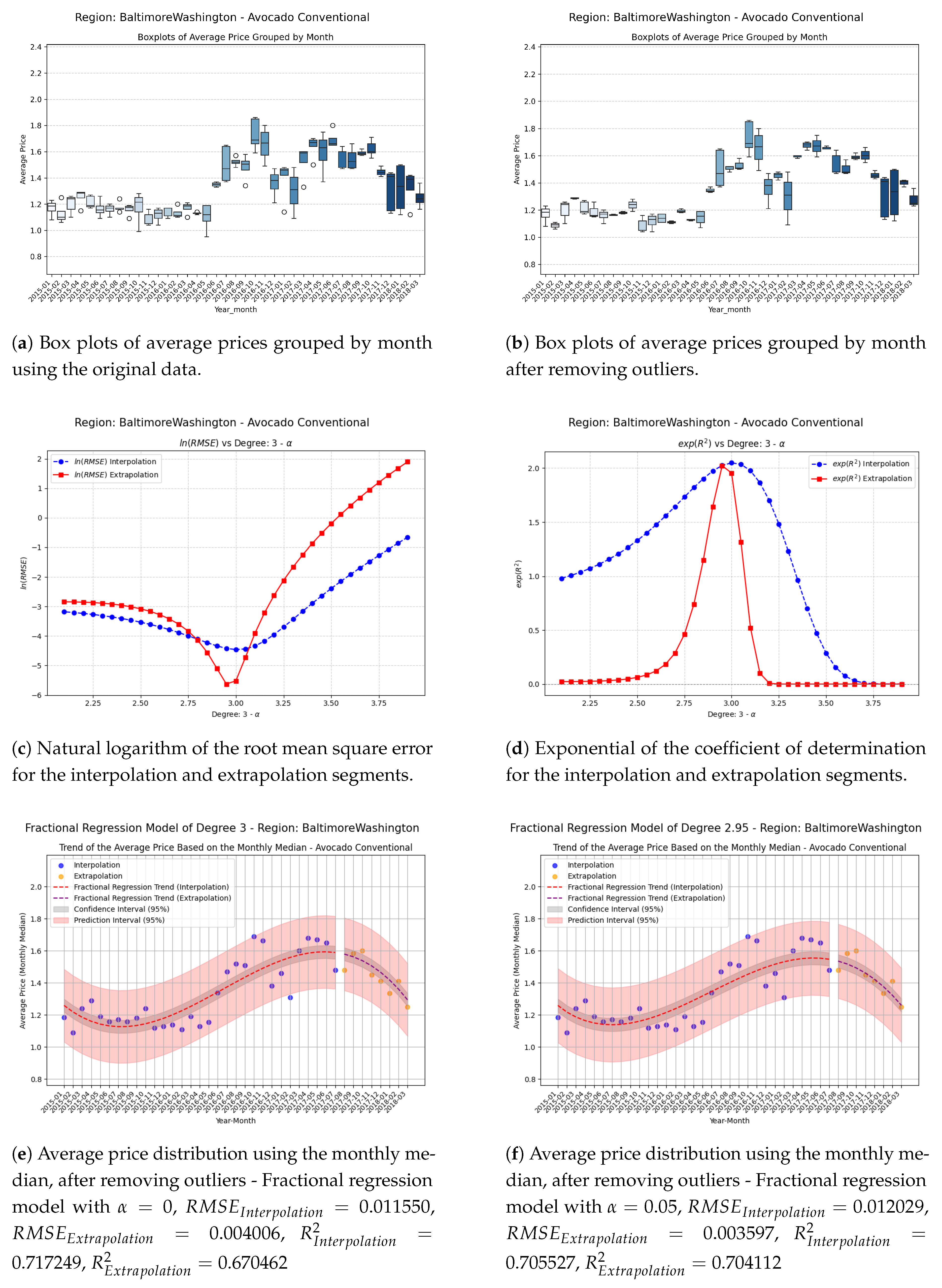
Figure 2.
Comparison of metrics and fractional regression models in the Chicago region.
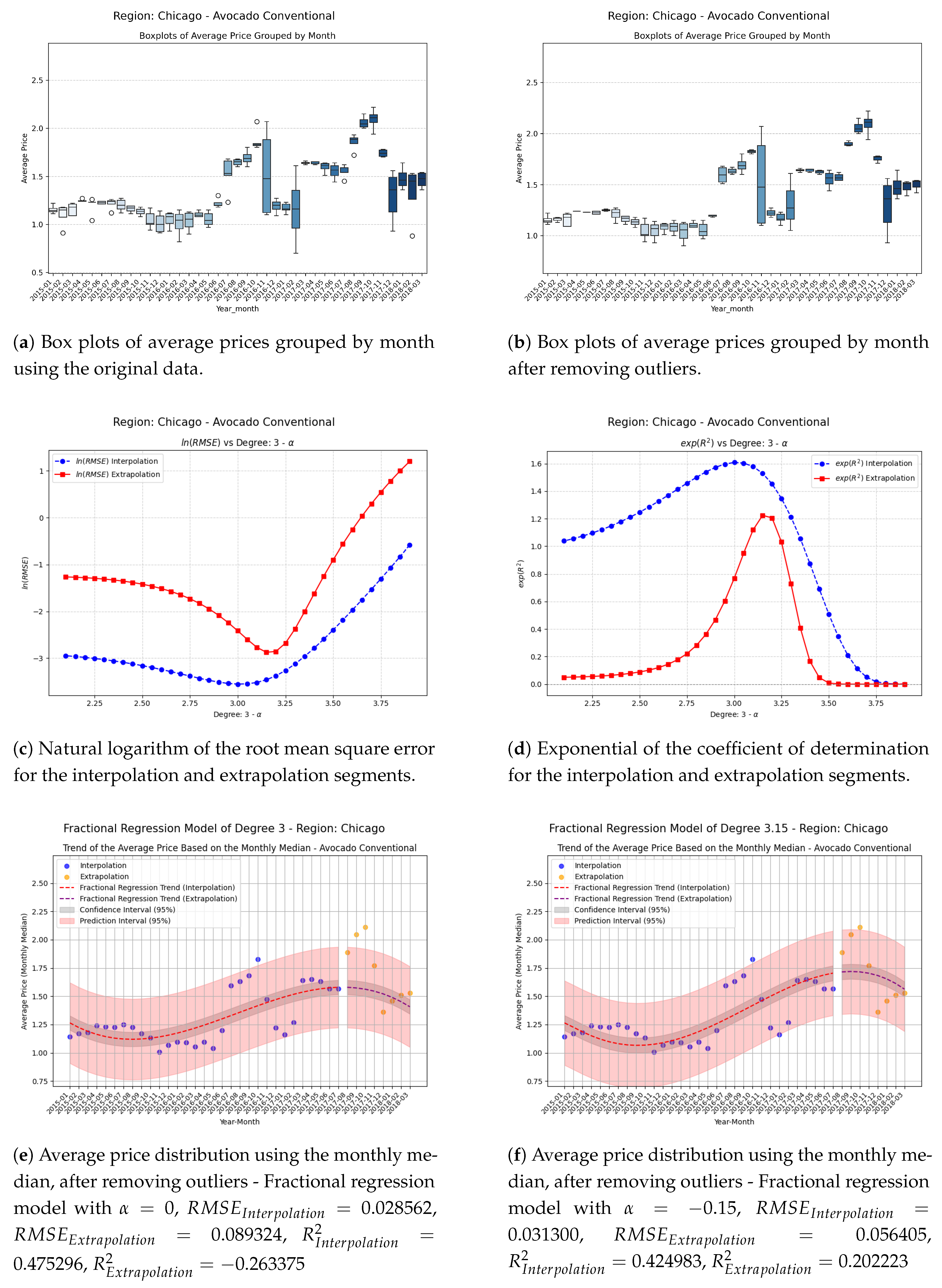
Figure 3.
Comparison of metrics and fractional regression models in the HartfordSpringfield region.
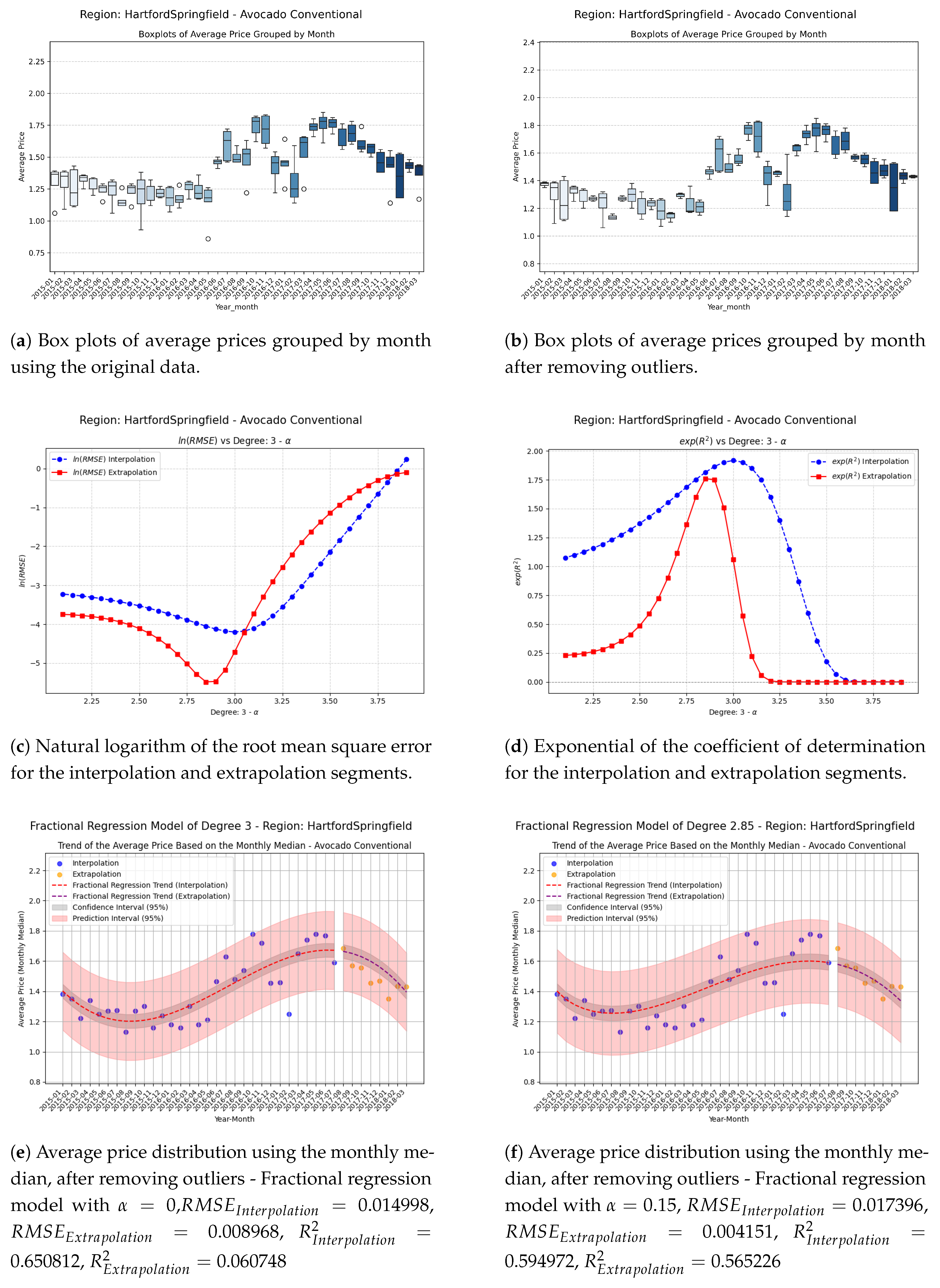
Figure 4.
Comparison of metrics and fractional regression models in the Midsouth region.
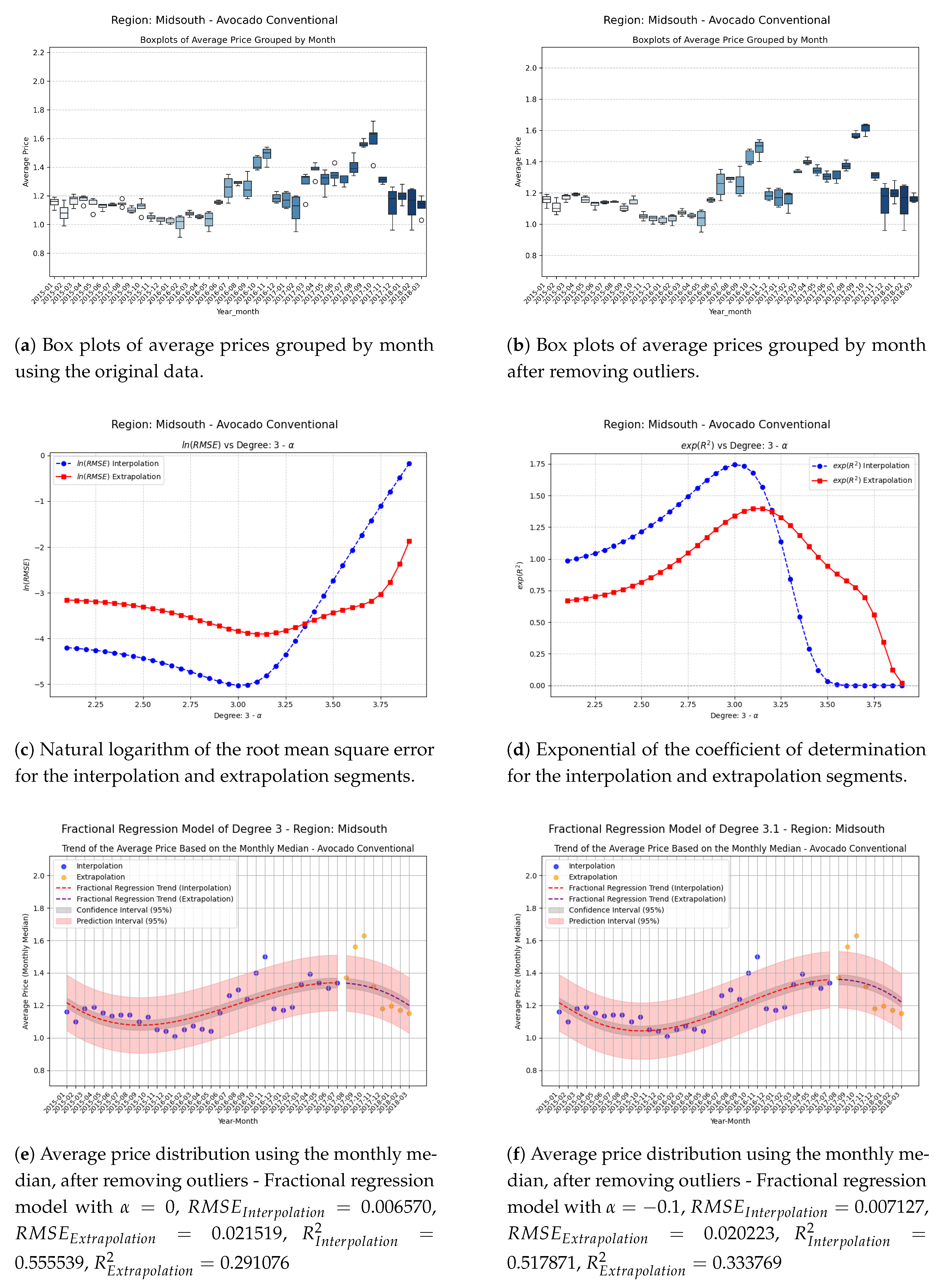
Figure 5.
Comparison of metrics and fractional regression models in the California region.
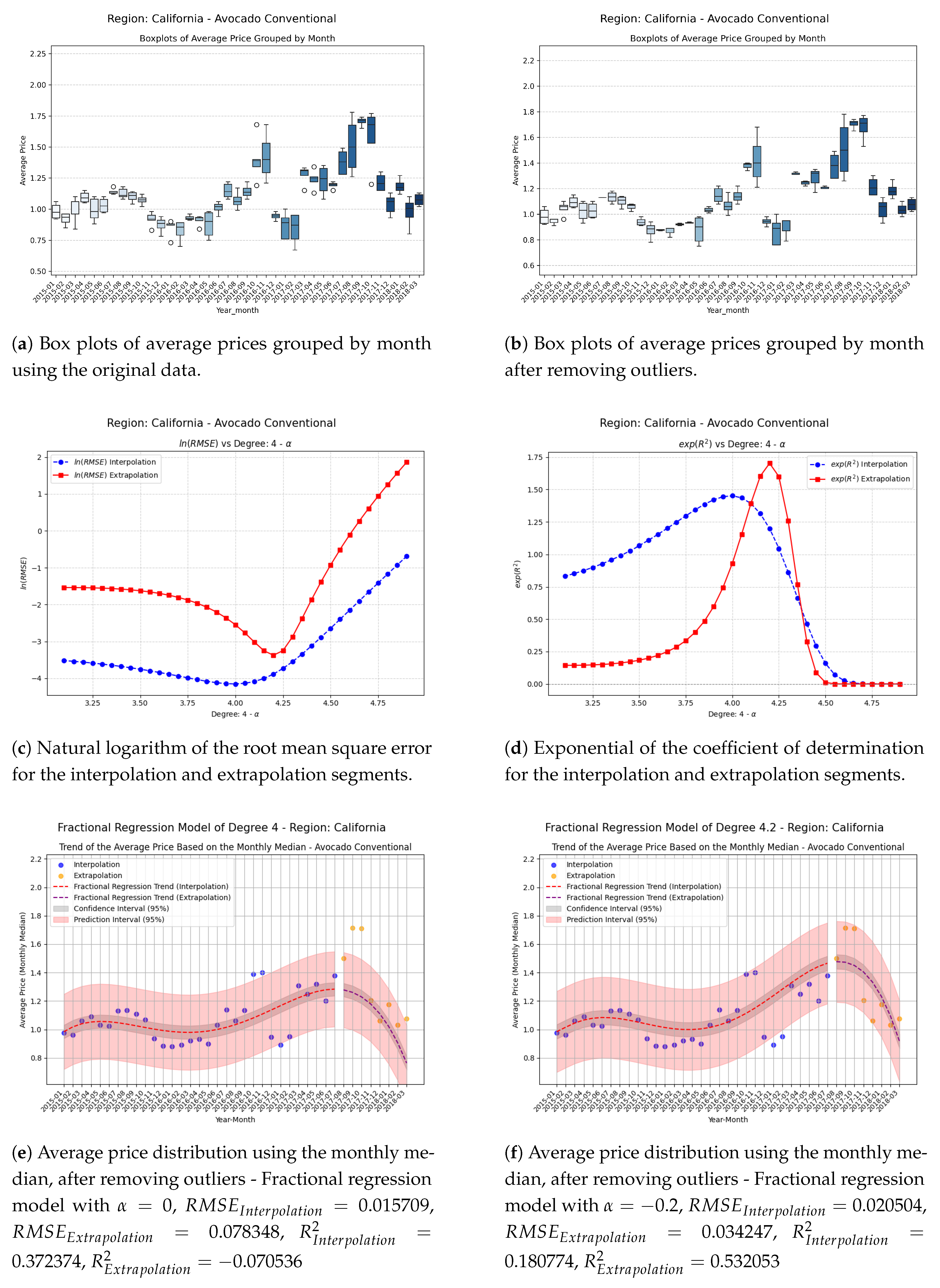
Figure 6.
Comparison of metrics and fractional regression models in the GrandRapids region.
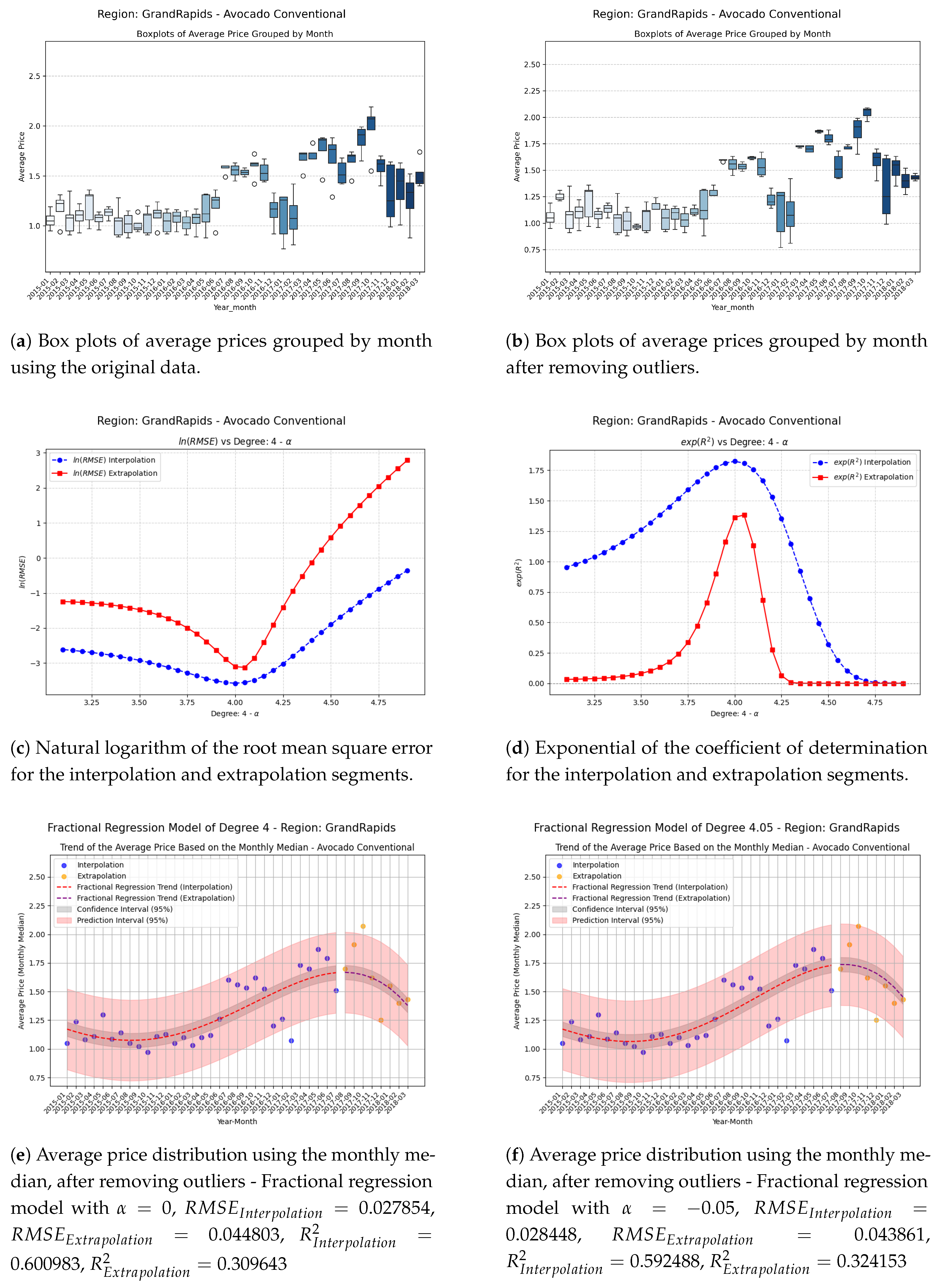
Figure 7.
Comparison of metrics and fractional regression models in the Louisville region.
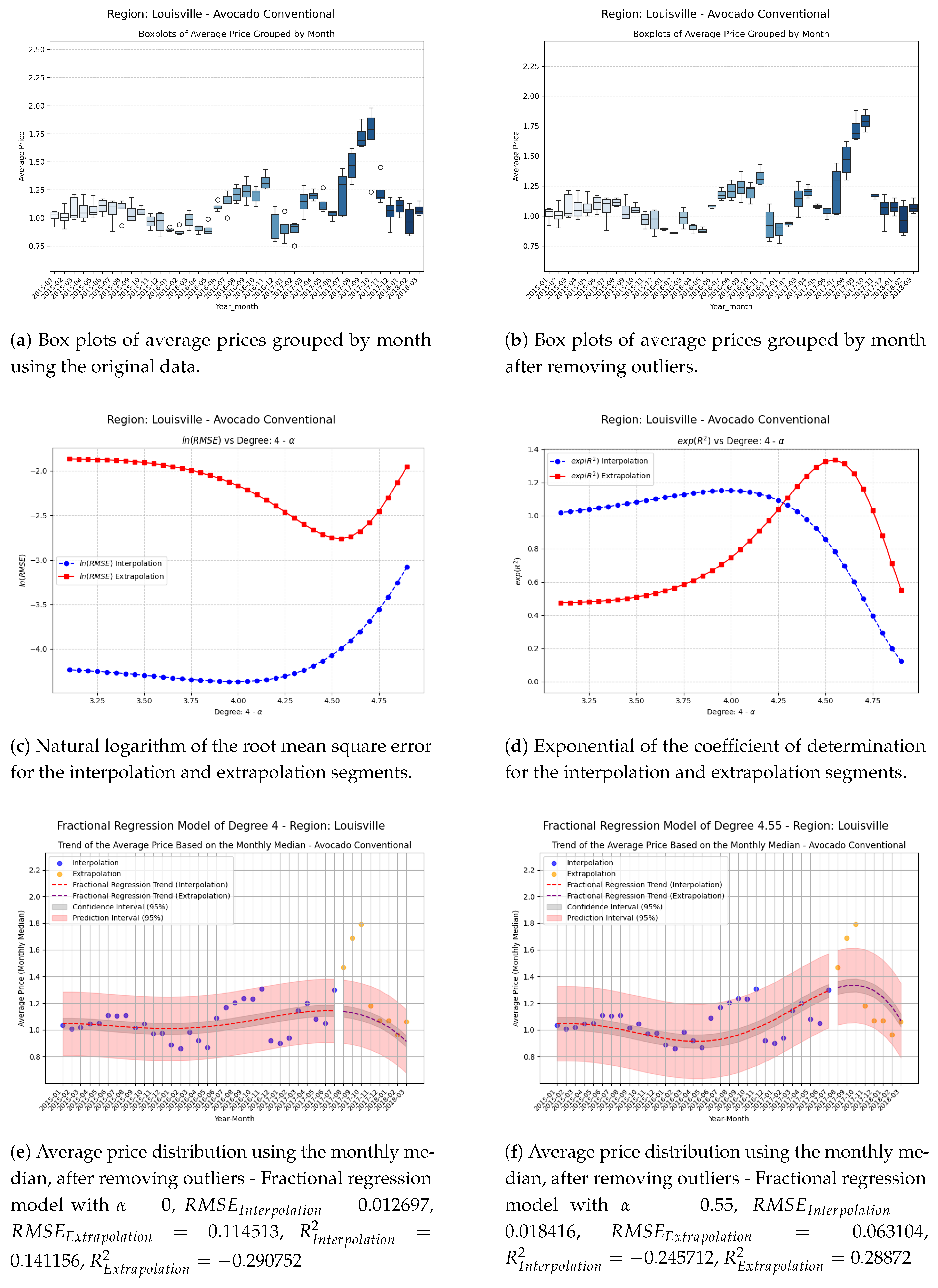
Figure 8.
Comparison of metrics and fractional regression models in the NorthernNewEngland region.
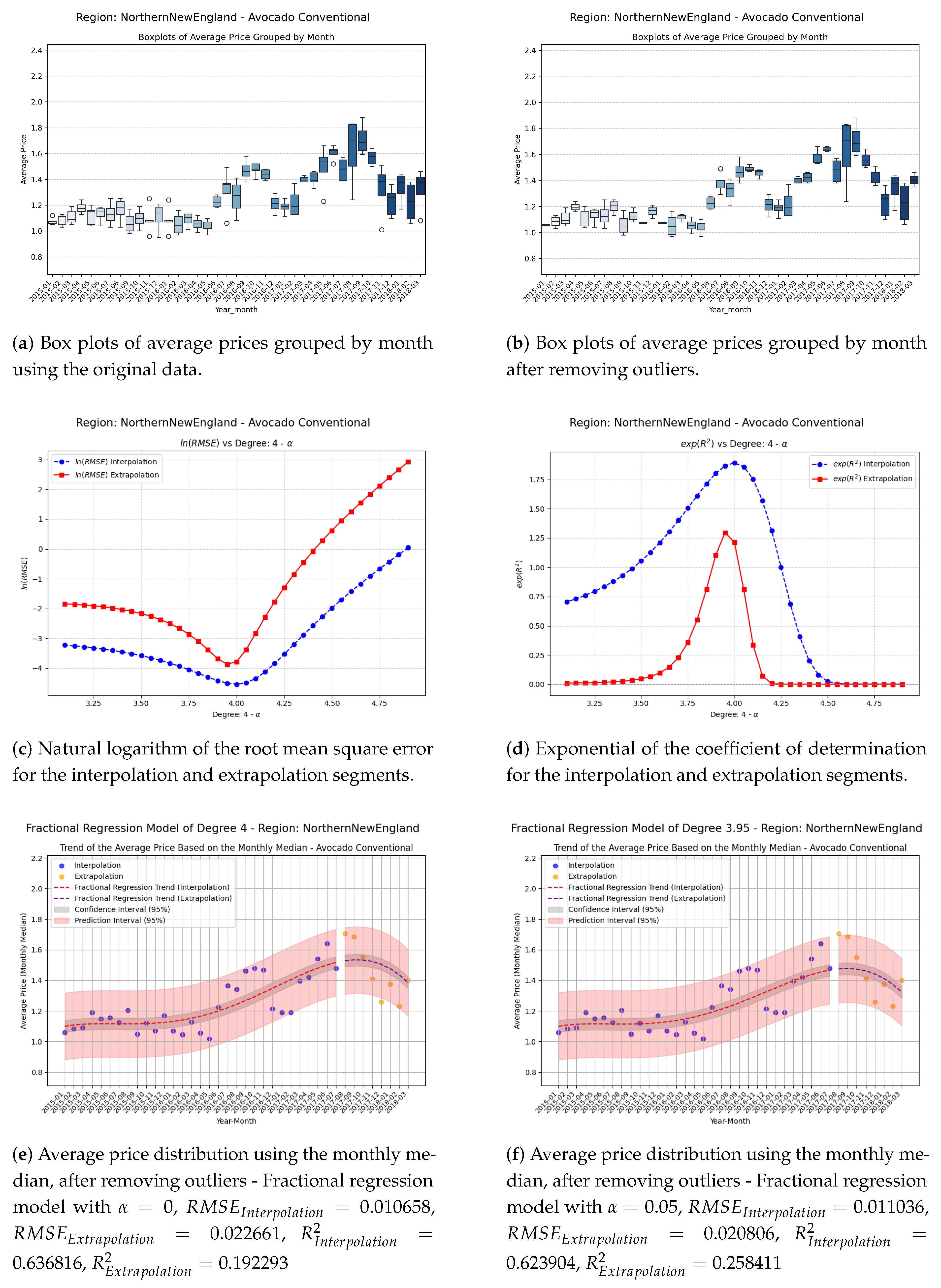
Figure 9.
Comparison of metrics and fractional regression models in the Plains region.
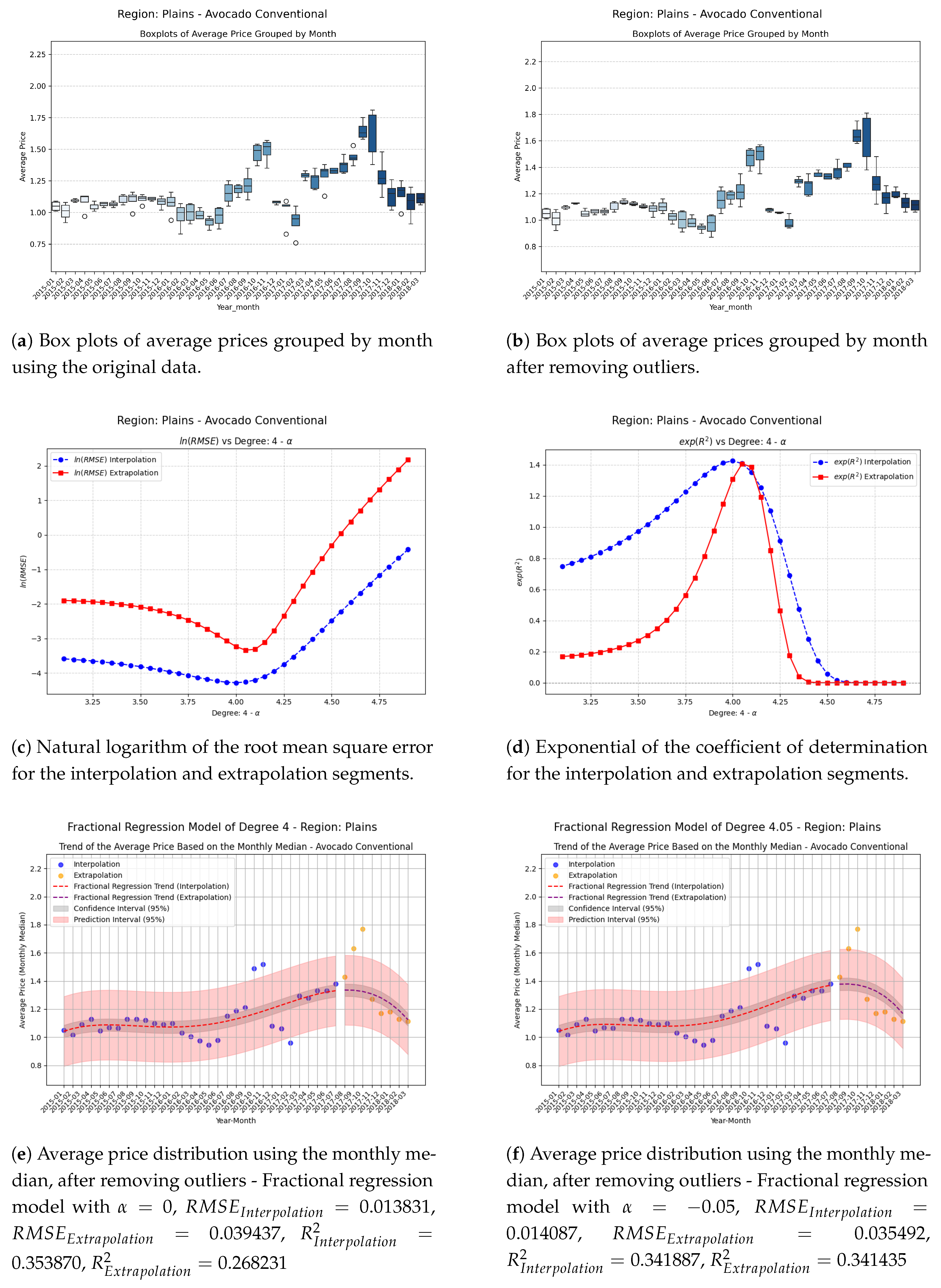
Figure 10.
Comparison of metrics and fractional regression models in the TotalUS region.
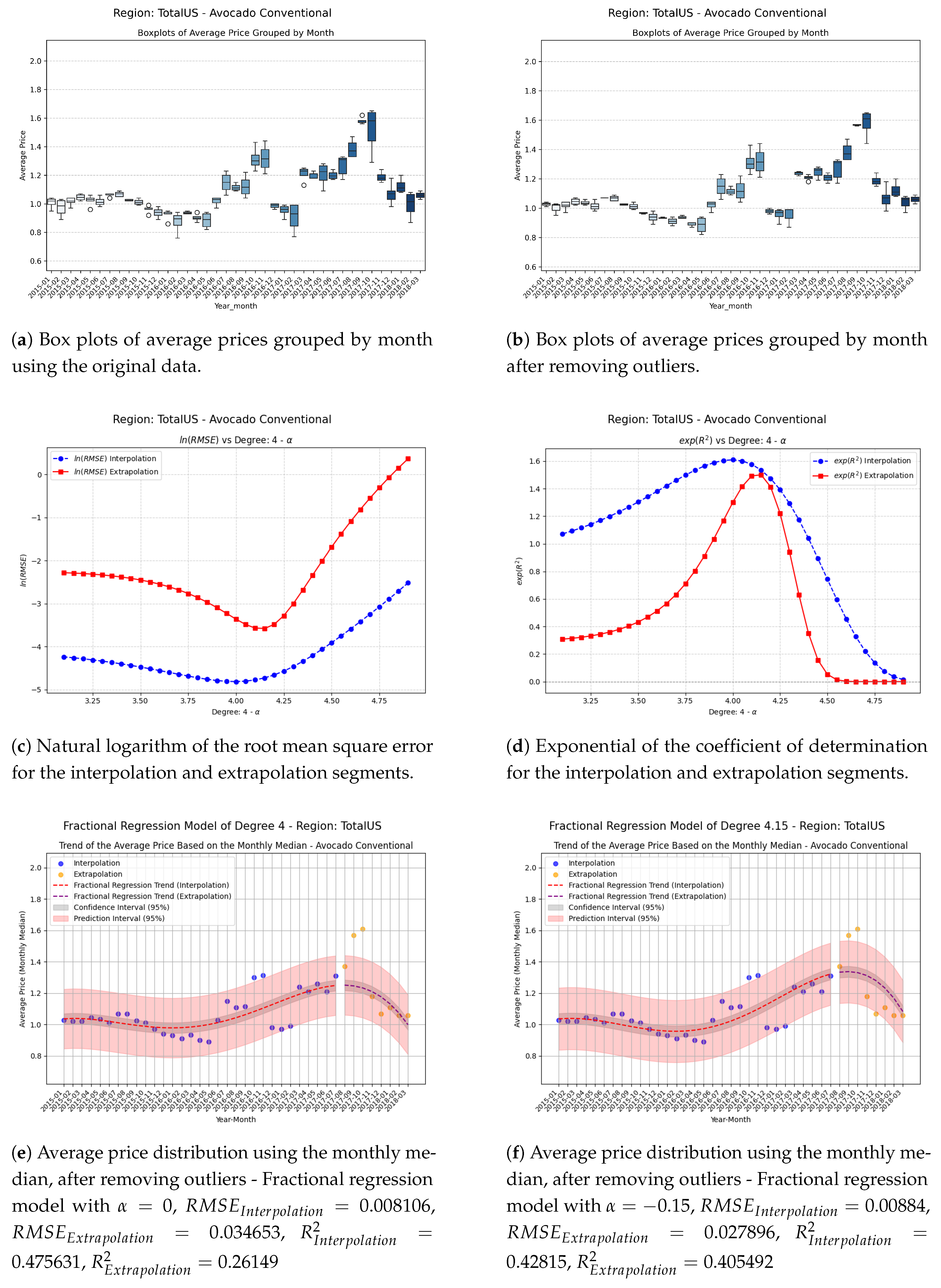
Figure 11.
Comparison of metrics and fractional regression models in the Boise region.
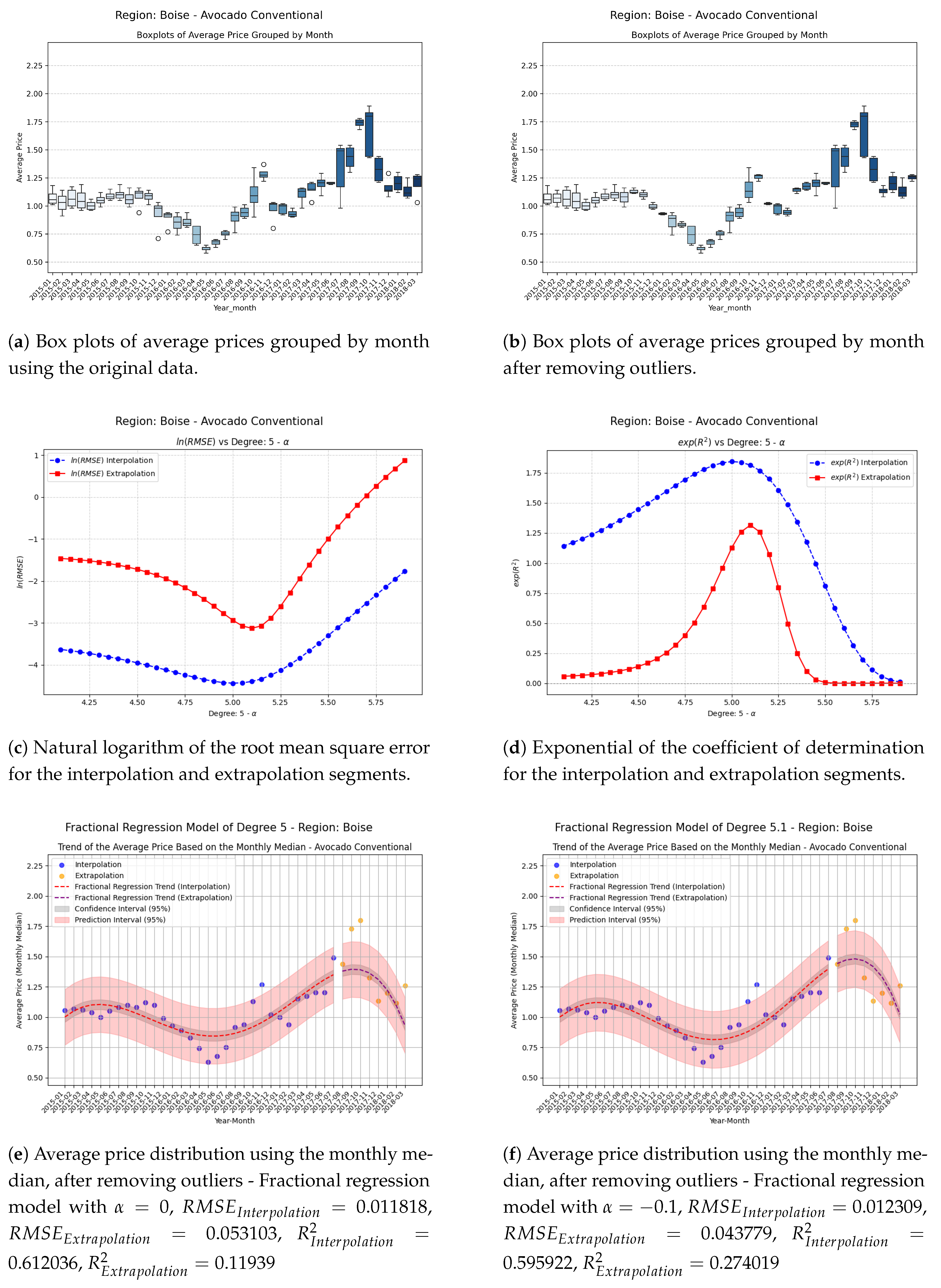
Figure 12.
Comparison of metrics and fractional regression models in the Jacksonville region.
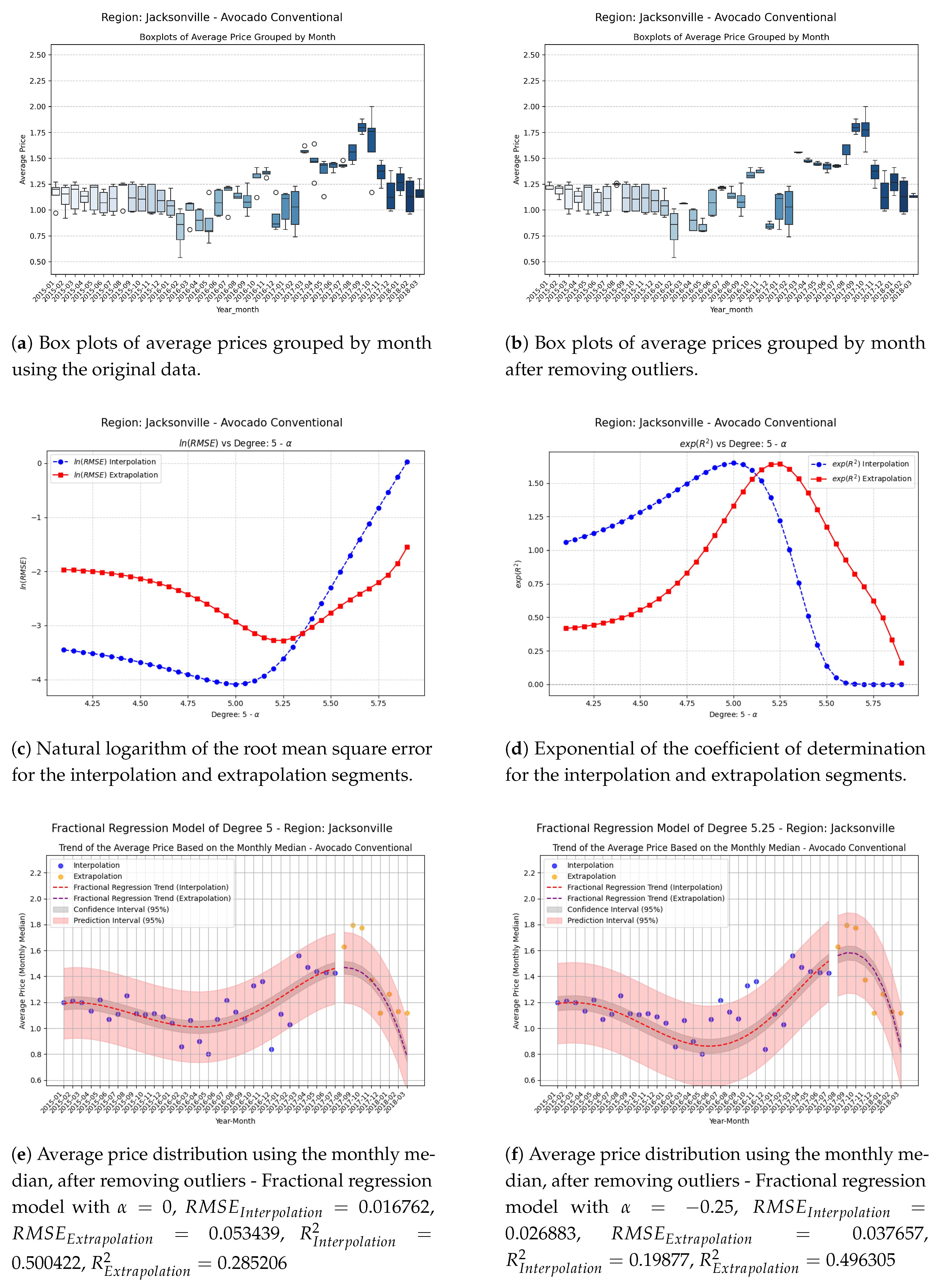
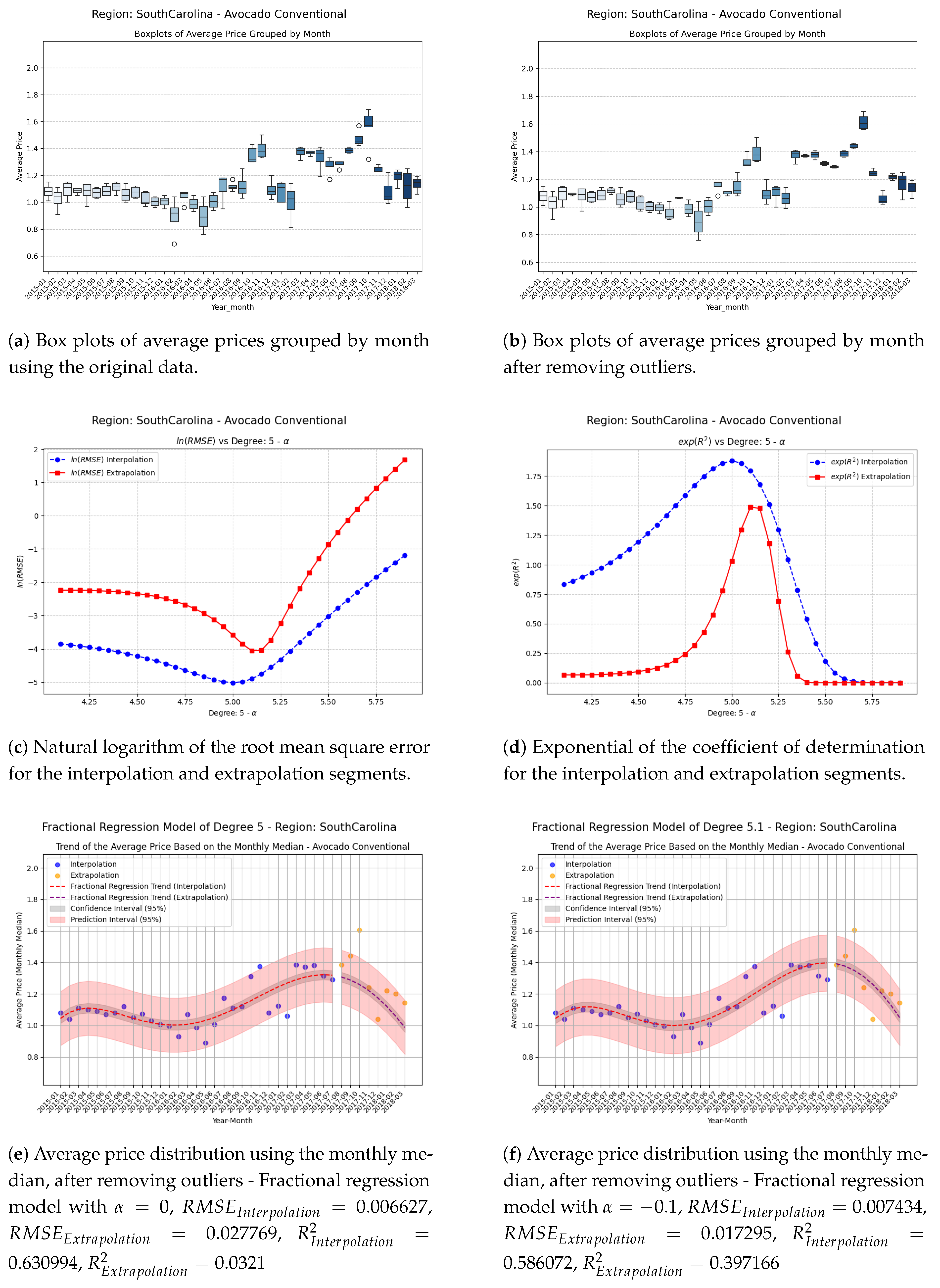
Figure 13.
Comparison of metrics and fractional regression models in the SouthCarolina region.
References
- Kenneth S. Miller and Bertram Ross. An introduction to the fractional calculus and fractional differential equations. Wiley-Interscience, 1993.
- Rudolf Hilfer. Applications of fractional calculus in physics. World Scientific, 2000.
- Keith Oldham and Jerome Spanier. The fractional calculus theory and applications of differentiation and integration to arbitrary order, volume 111. Elsevier, 1974.
- A.A. Kilbas, H.M. Srivastava, and J.J. Trujillo. Theory and Applications of Fractional Differential Equations. Elsevier, 2006.
- Edmundo Capelas De Oliveira and José António Tenreiro Machado. A review of definitions for fractional derivatives and integral. Mathematical Problems in Engineering, 2014. [CrossRef]
- G Sales Teodoro, JA Tenreiro Machado, and E Capelas De Oliveira. A review of definitions of fractional derivatives and other operators. Journal of Computational Physics, 388:195–208, 2019. [CrossRef]
- Duarte Valério, Manuel D Ortigueira, and António M Lopes. How many fractional derivatives are there? Mathematics, 10(5):737, 2022. [CrossRef]
- Ali Safdari-Vaighani, Alfa Heryudono, and Elisabeth Larsson. A radial basis function partition of unity collocation method for convection–diffusion equations arising in financial applications. Journal of Scientific Computing, 64(2):341–367, 2015. [CrossRef]
- A. Torres-Hernandez, F. Brambila-Paz, and C. Torres-Martínez. Numerical solution using radial basis functions for multidimensional fractional partial differential equations of type black–scholes. Computational and Applied Mathematics, 40(245), 2021. [CrossRef]
- Awa Traore and Ndolane Sene. Model of economic growth in the context of fractional derivative. Alexandria Engineering Journal, 59(6):4843–4850, 2020. [CrossRef]
- Inés Tejado, Emiliano Pérez, and Duarte Valério. Fractional calculus in economic growth modelling of the group of seven. Fractional Calculus and Applied Analysis, 22(1):139–157, 2019. [CrossRef]
- Emanuel Guariglia. Fractional calculus, zeta functions and shannon entropy. Open Mathematics, 19(1):87–100, 2021. [CrossRef]
- A. Torres-Henandez and F. Brambila-Paz. An approximation to zeros of the riemann zeta function using fractional calculus. Mathematics and Statistics, 9(3):309–318, 2021. [CrossRef]
- Eduardo De-la Vega, Anthony Torres-Hernandez, Pedro M Rodrigo, and Fernando Brambila-Paz. Fractional derivative-based performance analysis of hybrid thermoelectric generator-concentrator photovoltaic system. Applied Thermal Engineering, 193:116984, 2021. [CrossRef]
- A. Torres-Hernandez, F. Brambila-Paz, P. M. Rodrigo, and E. De-la-Vega. Reduction of a nonlinear system and its numerical solution using a fractional iterative method. Journal of Mathematics and Statistical Science, 6:285–299, 2020. ISSN 2411-2518.
- R Erfanifar, K Sayevand, and H Esmaeili. On modified two-step iterative method in the fractional sense: some applications in real world phenomena. International Journal of Computer Mathematics, 97(10):2109–2141, 2020. [CrossRef]
- Alicia Cordero, Ivan Girona, and Juan R Torregrosa. A variant of chebyshev’s method with 3αth-order of convergence by using fractional derivatives. Symmetry, 11(8):1017, 2019. [CrossRef]
- Krzysztof Gdawiec, Wiesław Kotarski, and Agnieszka Lisowska. Newton’s method with fractional derivatives and various iteration processes via visual analysis. Numerical Algorithms, 86(3):953–1010, 2021. [CrossRef]
- Krzysztof Gdawiec, Wiesław Kotarski, and Agnieszka Lisowska. Visual analysis of the newton’s method with fractional order derivatives. Symmetry, 11(9):1143, 2019. [CrossRef]
- Ali Akgül, Alicia Cordero, and Juan R Torregrosa. A fractional newton method with 2αth-order of convergence and its stability. Applied Mathematics Letters, 98:344–351, 2019.
- A. Torres-Hernandez and F. Brambila-Paz. Fractional Newton-Raphson Method. Applied Mathematics and Sciences: An International Journal (MathSJ), 8:1–13, 2021. [CrossRef]
- A. Torres-Hernandez, F. Brambila-Paz, U. Iturrarán-Viveros, and R. Caballero-Cruz. Fractional Newton-Raphson Method Accelerated with Aitken’s Method. Axioms, 10(2):1–25, 2021. [CrossRef]
- A. Torres-Hernandez, F. Brambila-Paz, and E. De-la-Vega. Fractional Newton-Raphson Method and Some Variants for the Solution of Nonlinear Systems. Applied Mathematics and Sciences: An International Journal (MathSJ), 7:13–27, 2020. [CrossRef]
- Giro Candelario, Alicia Cordero, and Juan R Torregrosa. Multipoint fractional iterative methods with (2α+ 1) th-order of convergence for solving nonlinear problems. Mathematics, 8(3):452, 2020. [CrossRef]
- Giro Candelario, Alicia Cordero, Juan R Torregrosa, and María P Vassileva. An optimal and low computational cost fractional newton-type method for solving nonlinear equations. Applied Mathematics Letters, 124:107650, 2022. [CrossRef]
- Francisco Damasceno Freitas and Laice Neves de Oliveira. A fractional order derivative newton-raphson method for the computation of the power flow problem solution in energy systems. Fractional Calculus and Applied Analysis, 27(6):3414–3445, 2024. [CrossRef]
- Thomas J Osler. Leibniz rule for fractional derivatives generalized and an application to infinite series. SIAM Journal on Applied Mathematics, 18(3):658–674, 1970. [CrossRef]
- Ricardo Almeida. A caputo fractional derivative of a function with respect to another function. Communications in Nonlinear Science and Numerical Simulation, 44:460–481, 2017. [CrossRef]
- Hui Fu, Guo-Cheng Wu, Guang Yang, and Lan-Lan Huang. Continuous time random walk to a general fractional fokker–planck equation on fractal media. The European Physical Journal Special Topics, pages 1–7, 2021. [CrossRef]
- Qin Fan, Guo-Cheng Wu, and Hui Fu. A note on function space and boundedness of the general fractional integral in continuous time random walk. Journal of Nonlinear Mathematical Physics, 29(1):95–102, 2022. [CrossRef]
- M Abu-Shady and Mohammed KA Kaabar. A generalized definition of the fractional derivative with applications. Mathematical Problems in Engineering, 2021. [CrossRef]
- Khaled M Saad. New fractional derivative with non-singular kernel for deriving legendre spectral collocation method. Alexandria Engineering Journal, 59(4):1909–1917, 2020. [CrossRef]
- Mohamad Rafi Segi Rahmat. A new definition of conformable fractional derivative on arbitrary time scales. Advances in Difference Equations, 2019(1):1–16, 2019. [CrossRef]
- J Vanterler da C Sousa and E Capelas De Oliveira. On the ψ-hilfer fractional derivative. Communications in Nonlinear Science and Numerical Simulation, 60:72–91, 2018.
- Fahd Jarad, Ekin Uğurlu, Thabet Abdeljawad, and Dumitru Baleanu. On a new class of fractional operators. Advances in Difference Equations, 2017(1):1–16, 2017.
- Abdon Atangana and JF Gómez-Aguilar. A new derivative with normal distribution kernel: Theory, methods and applications. Physica A: Statistical mechanics and its applications, 476:1–14, 2017. [CrossRef]
- Mehmet Yavuz and Necati Özdemir. Comparing the new fractional derivative operators involving exponential and mittag-leffler kernel. Discrete & Continuous Dynamical Systems-S, 13(3):995, 2020. [CrossRef]
- Jian-Gen Liu, Xiao-Jun Yang, Yi-Ying Feng, and Ping Cui. New fractional derivative with sigmoid function as the kernel and its models. Chinese Journal of Physics, 68:533–541, 2020. [CrossRef]
- Xiao-Jun Yang and JA Tenreiro Machado. A new fractional operator of variable order: application in the description of anomalous diffusion. Physica A: Statistical Mechanics and its Applications, 481:276–283, 2017. [CrossRef]
- Abdon Atangana. On the new fractional derivative and application to nonlinear fisher’s reaction–diffusion equation. Applied Mathematics and computation, 273:948–956, 2016. [CrossRef]
- Ji-Huan He, Zheng-Biao Li, and Qing-li Wang. A new fractional derivative and its application to explanation of polar bear hairs. Journal of King Saud University-Science, 28(2):190–192, 2016. [CrossRef]
- Ndolane Sene. Fractional diffusion equation with new fractional operator. Alexandria Engineering Journal, 59(5):2921–2926, 2020. [CrossRef]
- A. Torres-Hernandez and F. Brambila-Paz. Sets of fractional operators and numerical estimation of the order of convergence of a family of fractional fixed-point methods. Fractal and Fractional, 5(4):240, 2021. [CrossRef]
- A. Torres-Hernandez, F. Brambila-Paz, and R. Montufar-Chaveznava. Acceleration of the order of convergence of a family of fractional fixed point methods and its implementation in the solution of a nonlinear algebraic system related to hybrid solar receivers. Applied Mathematics and Computation, 429, 2022. [CrossRef]
- Anthony Torres-Hernandez, Fernando Brambila-Paz, and Rafael Ramirez-Melendez. Abelian groups of fractional operators. Computer Sciences & Mathematics Forum, 4(1), 2022. [CrossRef]
- A. Torres-Hernandez. Code of a multidimensional fractional quasi-Newton method with an order of convergence at least quadratic using recursive programming. Applied Mathematics and Sciences: An International Journal (MathSJ), 9:17–24, 2022. [CrossRef]
- Anthony Torres-Hernandez, Fernando Brambila-Paz, and Rafael Ramirez-Melendez. Proposal for use of the fractional derivative of radial functions in interpolation problems. Fractal and Fractional, 8(1):16, 2023. [CrossRef]
Disclaimer/Publisher’s Note: The statements, opinions and data contained in all publications are solely those of the individual author(s) and contributor(s) and not of MDPI and/or the editor(s). MDPI and/or the editor(s) disclaim responsibility for any injury to people or property resulting from any ideas, methods, instructions or products referred to in the content. |
© 2025 by the authors. Licensee MDPI, Basel, Switzerland. This article is an open access article distributed under the terms and conditions of the Creative Commons Attribution (CC BY) license (http://creativecommons.org/licenses/by/4.0/).
Copyright: This open access article is published under a Creative Commons CC BY 4.0 license, which permit the free download, distribution, and reuse, provided that the author and preprint are cited in any reuse.


