
Submitted:
20 April 2025
Posted:
21 April 2025
You are already at the latest version
Abstract
Building upon prior work this paper examines the business cycle from the perspective of the economy’s ability to process information. Specifically, the ratio of information to be processed divided by the economy’s capacity to process that information (R/C) is empirically derived and studied. This ratio undergoes an intuitive evolution over business cycles providing /a new method of understanding the economy’s present and future states. Additionally, insightful parallels to recently derived computational limits and scaling laws from large neural network models are presented. Finally new warning signs of the end of the business cycle and new sources of economic shocks are explained. This perspective offers new tools for monitoring the health of the economy and a new means for corrective policy interventions by fiscal and monetary authorities.
Keywords:
Business Cycle
; Yield Curve
; Information Processing Cycle
; Artificial Intelligence
; Entropic Yield Curve
; Scaling Laws
; Bear Market
; Neural Networks
1. Introduction
This paper will start with an introduction of the economy’s information processing cycle through the perspective of the ratio R/C expanding upon ideas from Parker (2017), (2018), and (2019). Next the historical evolution of R/C over the last several cycles will be studied with a particular emphasis on cycle end and the warning signals of an impending bear market. This is followed by a deeper examination of R/C through the lens of the limits of information processing and the statistical implications of those limits. Additionally, a new economic scaling law is derived and compared to those found in the training of large neural network models. Finally new fiscal and monetary policies are proposed based on these new tools to more optimally manage business cycles.
Several authors have studied the connections between the economy and its computational capacity. Lautsch (1983) explored the connections between the efficiency of information processing and an economy’s ability to create wealth, while Huberman (1996) attempted to use market mechanisms to understand computer dynamics. The effects of information and communication technology diffusion on the economic growth were studied by (Bahrini & Qaffas, 2019).
In Parker (2017) and (2018) the author studied the business cycle from the perspective of the limits of information processing. Specifically, these articles demonstrated that the observed structures and evolution of the yield curve over business cycles could be explained by changes in the economy’s information processing cycle and ratio R/C.
Additionally, various researchers have studied the empirical scaling laws for the training of large neural network models. Specifically, researchers such as (Kaplan et al., 2020), (Henighan et al., 2020), and (Hoffman et al., 2022) examined the dependence of the errors generated in the training of large neural network models on model size, dataset size, and the amount of compute available. They found trade-offs and scaling laws governing the relationships between these three variables and AI model training results and errors. A similar scaling law and set of relationships are derived empirically for the economy as a whole in this paper.
At the beginning of the last three business cycles a scaling law similar to the relation discovered by (Kaplan et al., 2020) appears to hold. It governs the proportion of data relative to the compute resources observed at business cycle start. Unlike AI models market participants have little knowledge or control of the economy’s levels of the three inputs: dataset size, model complexity, and total available compute. As empirically demonstrated over several business cycles the economy’s data size relative to its total available compute available repeated starts at a fixed proportion of compute available and falls as learning takes place and the available data is consumed. This gradual reduction in the ratio R/C drives the evolution of the business cycle and is a limit on its duration.
2. Results
Parker (2017), (2018) examined the information processing ratio R/C over various business cycles as presented in Figure 1 (See section 4 for details on the empirical derivation of R/C and precise variable definitions). As seen below R/C seems to be a mirror image the SP500 over the 35 years studied from 1990 through the end of 2024. The peaks of R/C correspond to the troughs of the SP500 over three full business cycles. At the beginning of the business cycles the Sp500 begins its climb from the most recent trough while R/C begins to decline from its maximum. While the SP500 seems to have no lower or upper limits (except the trivial ultimate lower bound of 0), R/C seems bounded by a maximum and a minimum near cycle end. Additionally, it was found that at the end of each cycle when R/C falls to approximately 1 and the variance of R/C spikes the business cycle soon ends, and equity bear markets begin.
To further examine the role and structure of the information processing ratio R/C we will examine it through the lens of Figure 2, which provides a visual representation of the relationship between R and C over a business cycle. At cycle start companies utilize the best information processes, organizational structures, and models available. When a new cycle starts as indicated by the left side of the diagram, there is a larger set of information R is available than was available under during the prior cycle. However, the economy as a whole is not yet ready or knowledgeable of how to process all of this new excess information and can only fully utilize and process a subset , of the total available bandwidth . As the business cycle progresses companies throughout the economy gain more knowledge and expertise with the new information set and gradually expand . This is observed empirically as a gradual decrease in the ratio R/C over time. Eventually the economy reaches the level of R/C = 1 where all available and relevant information is being processed with a nonzero error σ and .
When R = C, information is being processed at the maximum capacity possible, however no company individually or collectively will know precisely when they or the larger economy reaches this balanced point. Both individually and collectively companies will move slightly past R/C = 1 due to competitive pressures, always attempting to process more information at the fastest rate possible. As R/C declines companies and the economy move into a less efficient information processing regime signified by R’+ R > R. R’+R represents an expansion in the total volume of information processed beyond R. This expansion is facilitated by either lagging information processing or substituting new variables for those already optimally in R. This is evidenced by R/C dipping below 1 near the end of past cycles. Only when companies can empirically observe their diminishing returns (i.e. more errors, reduced output, or lower profits) is the need for more significant changes in their information processing structures evident. At this point the information processing cycle starts again with new technology including greater compute, larger datasets, and more powerful explanatory models at R/C ≈ 1.27.
One exception to the process observed over the past 35 years is the March 2020 economic downturn. The Covid induced recession is more akin to the economy being suddenly shut off and not a more typical type of recession. During this event the economy did enter recession after the usual drop of R/C to near 1 simultaneously with a large increase in the variance of R/C. However, the economy did not reset to R/C = 1.27 as it did in the previous 3 cycles upon reopening. This is theorized to be due to the incomplete processing of the full information set R available at the time of the abrupt economic shutdown. Once the economy reopened the information processing cycle already in progress resumed and continued through the studied time period. This information processing perspective gives a projection of the economy’s evolution based on the amount of information left to be exploited with a given level of technology. This is analogous to measuring the driving distance of a car with a given amount of fuel. An exogenous shock like the Covid incident is akin to the fuel being shut off to engine and the car stopping. Once the fuel is again available the car can continue driving until the fuel is fully consumed. Similarly, once the economy reopened the information processing continued from the point where it left off towards information exhaustion and full cycle completion.
2.1. Relative Sample Size
To further facilitate the discussion, R/C will be examined from a simple but important statistical perspective. Most statistical analysis assumes a random sample drawn from an infinite population (or equivalently sampling from a finite population with replacement). However, the data needed to calculate the future state of the economy (R) is large but finite, as is the proportion of that data utilized in the computations (R/C).
When samples are drawn from a finite population (without replacement for each economic actor individually) estimates of measures such as the sample variance can be will be overstated if the sample size is a significant proportion of the overall population. As described by (Cochran 24/1977) the finite population correction factor is presented below where N is the population size and n is the sample size. This factor is multiplied by the variance. The larger the sample size n relative to the population N the smaller the true variance.
Next the relative sample size analysis is extended with the help of Figure 2. The behavior of R and C can be divided into two main periods when R/C > 1 and R/C < 1. When R/C > 1, R is constant but the amount of the total available compute grows from C = R/1.27 to where . The variance during this period is described by equation 1 below:
Beginning of Cycle when R/C >1, R is constant and C rises gradually to
The latter part of cycle is illustrated by equation 2. The economy passes the point where R = C. At this stage R/C < 1, C is constant at , and R(t) is now variable due to the addition of R’ or the substitution of elements of R with those of R’. With the substitution and/or the addition of R’ to R, the true R utilized for computations is reduced leading to greater variance of R/C. Substitution of the R’ values for R leads to a direct reduction in the R available for computations. While addition of R’ leads to more data than can be utilized since R = which also will lead to a reduction in available R.
R(t) = R-R’(t); subtraction and/or addition of R’ reduces the true R utilized
The key takeaway is as R/C declines, relatively more of the available population data is properly sampled and used in the economy’s computation of the next state. At the beginning of the business cycle R > C, and the variance of R/C will be larger than later in intermediate parts of business cycle when companies are able to accurately process a larger percentage of the available data. Over time as companies learn, this growing level of the proper utilization of the available data (or an increase in relative sample size) leads to a decrease in the variance of R/C as seen in Parker (2018) and (2019).
Eventually R/C falls to 1 where the economy is processing all of the available and relevant information R, and the variance of R/C reaches a minimum. This is the point of minimum variance and error production in the economy’s information processing during the business cycle. Companies individually and the economy as a whole are not aware of when they reach the point where R/C = 1. Due to this ignorance and competitive pressures companies will continue to expand information processing until they pass this point and the ratio descends to R/C < 1. As R/C declines below 1 there is a increase in the variance of R/C and of error production in information processing. At this point companies begin to become aware of the need to expand both R and C. When enough of the economy’s companies make this switch to more powerful models, larger datasets, and higher total compute a new cycle begins typically with R/C ≈ 1.27 as seen in the last few business cycles over the 35 years studied.
The multiscale nature of economic information processing was studied in Parker (2024). Specifically, it was found that the shorter information processing timescales have the greatest influence on economic dynamics. The information content of the shortest timescales will be exploited well before that of longer timescales. In essence the economy with its current level of technological development will exhaust learning at the shortest timescales first. This leads to a collapse of learning first at the shorter timescales and then at increasingly larger timescales as the information content progressively is exhausted. To return to higher levels of productive information processing new technologies (greater compute, larger datasets, and new more powerful theoretical models) must be embraced at the start of the next business cycle Parker (2024).
2.2. Constrained Compute and Error Growth over the Business Cycle
The effects of the change in R/C empirically from approximately R/C = 1.27 at cycle start to R/C < 1 at cycle end in the past few business cycles can also be examined from the growth of error in information processing.
(Kaplan et al., 2020), (Henighan et al., 2020), and (Hoffman et al., 2022) examined the effect of holding total compute constrained while searching for the optimal model and datasize in large neural network training experiments. They found that there is a tradeoff between model, data, and fixed compute size when measured in terms of model training loss or minimum model error. A similar tradeoff is seen in the economy’s optimal allocation of data, model and compute as measured by R/C as illustrated in Figure 3 and empirically seen by the parabolic variances of R/C in Figure 4.
In Figure 4 the variance of R/C over the time full time period 1990 -2024 is presented. Note the spikes at the end/start of each business cycle and the lower variance levels in between the spikes. This structure of the variance of R/C corresponds to the structure of parabolic errors found for large neural networks. This will be explored more in the next section.
(Kaplan et al., 2020), (Henighan et al., 2020), and (Hoffman et al., 2022) also studied the effects on large scale AI models of holding the compute available constant while varying the model and/or dataset size. The parabolic isocompute curves as seen in Figure 4 are the result of this tradeoff. The minimum of these curves represents the dataset and/or model size with the lowest training data loss or error for a fixed or maximum level of total available compute.
2.3. R/C over Multiple Cycles
Over multiple business cycles it is theorized that economy experiences isocompute curves similar to the isocompute curves seen in AI training applications (Kaplan et al., 2020), (Henighan et al., 2020), and (Hoffman et al., 2022). Assuming that the total compute available increases meaningfully from one cycle to the next, new lower isocompute parabolas with declining minimum errors would be expected as illustrated in Figure 5, similar to those seen in the previously cited references. In Figure 6, the US economy’s actual computational error (σ) from equation 3 is empirically estimated over the past 3 business cycles. This error estimate is found to be declining as expected supporting the hypothesis of increasing total available computation and declining errors (σ- values) over multiple cycles.
There are two relevant types of errors or information loss experienced by the economy over a business cycle in terms of information processing. The first occurs in the computations that the economy as a whole and its individual economic actors perform to determine the next state of the economy. This is analogous to the training loss in the large AI models.
The second is due to the increases in the variability of R/C. The rise in the variance of R/C increases the variance of interest rates and ultimately inflation. The rise in interest rate volatility increases inflationary pressures in a variety of ways. Menu costs will increase as prices fluctuate and decrease the stability of relative prices. As menu costs rise firms while need to update their prices more frequently, these rapidly fluctuating relative prices can lead to a misallocation of resources. Further exacerbating overall instability and inflationary pressures are the differential price adjust speeds. Some prices adjust rapidly to interest rate changes and others at a lag. This will cause intertemporal relative prices to fluctuate more erratically as interest rate volatility rises. These increased inefficiencies all lead to further decreases in economic efficiency, reductions in output and purchasing power, and increases in the inflation rate.
Figure 5 illustrates the concept of increasing isocompute curves caused by increases in total compute over business cycles. Figure 6 presents the estimated values of the US economy’s computational error over the studied business cycles. Using the entropic yield curve equation 3 and solving for using the 3-month timescale, an estimate of the economy’s computational error is presented in Figure 6 1. Similar to large scale AI models, with increasing data the economy’s error rate appears to fall over the various business cycles as highlighted by the declining values over time and the fitted trend line. A trend such as this is to be expected if the economy is growing its compute and data capacity between business cycles.
2.4. US Economy’s Scaling Law at Cycle Start
(Kaplan et al 2020), (Henighan et al. 2020), and (Hoffman et al. 2022) examined scaling laws of various AI training models they studied. Of particular interest to this study was the scaling law presented on page 3, and in Table 6 of Appendix A of (Kaplan et al., 2020) and Table 2 and Table A2 and Figure A2 of the Appendix of (Hoffman et al., 2022) given its focus on the relationship between dataset size and the total available compute. The relation states that optimal dataset size is proportional to total compute by the factor .
A similar optimization appears to occur at the beginning of each business cycle. This is evidenced by R/C = 1.27 at each cycle start.
For simplification setting the constant and rearranging terms
Comparing
It is not surprising that at cycle start businesses individually and the economy as a whole expand their dataset sizes, model sizes and total compute to an optimal allocation. After the start of the cycle other forces dictate the evolution of these inputs but at cycle start the various market participants are able to setup these initial allocations optimally.
3. Discussion of Central Government and Monetary Policy
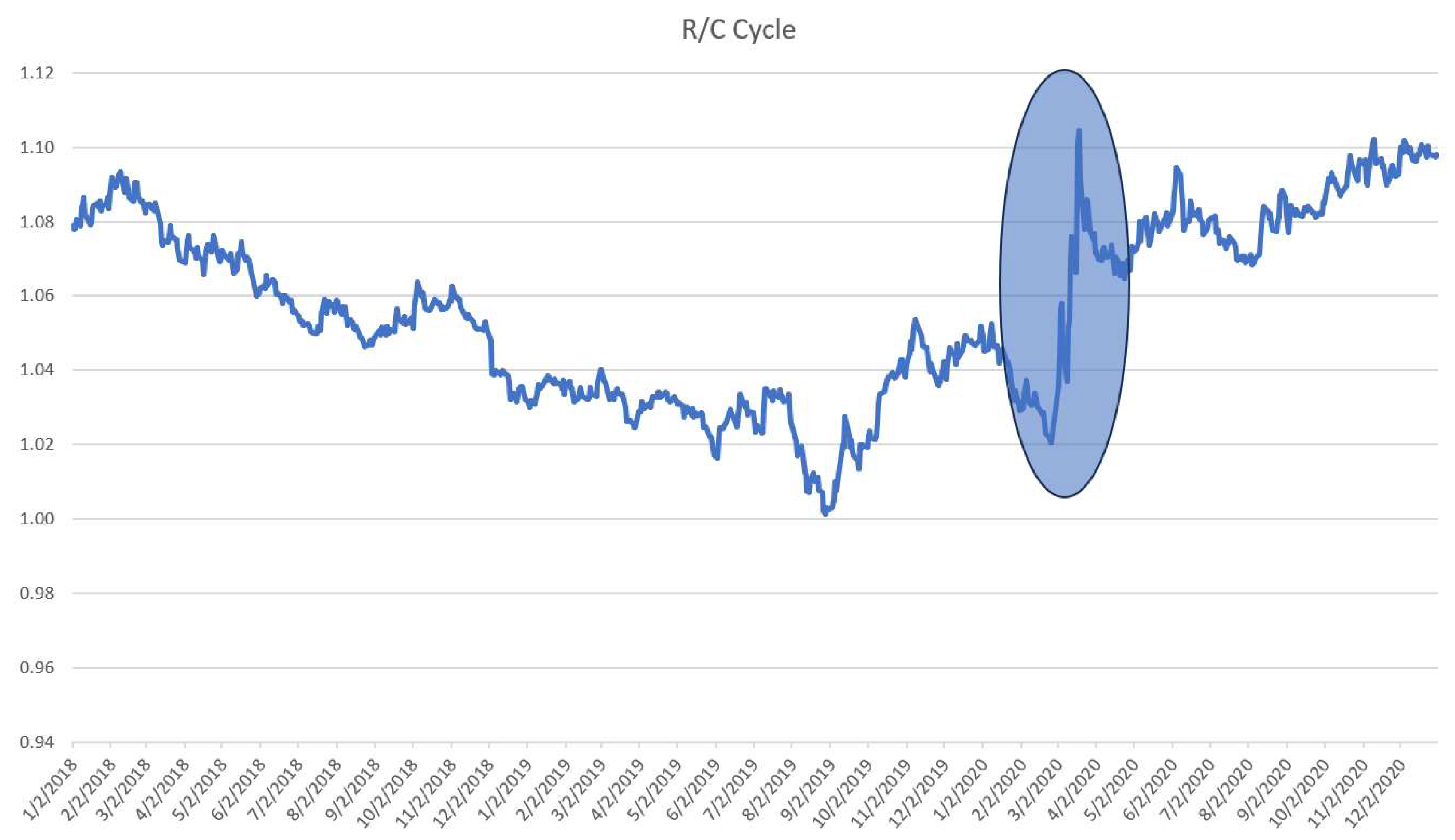
There are a variety of information processing shocks possible that may impact the overall economy. These can include information shocks and compute availability shocks that shift the level of R/C either positively or negatively. The impact of the onset of covid on the economy in March 2020 resulted in a large upward shift in R/C as seen in Figure 7. With the onset of the covid pandemic extreme uncertainty was injected into the economy. This growth in uncertainty represented a large increase in the amount of data that needed to be processed which pushed R/C upward.
Compute shocks on the other hand could come from the lack of the availability of high demand AI microchips for instance leading to a constraint on the growth of total compute. In addition to abrupt upward or downward shifts in R/C, less dramatic changes in information or available compute could also lead to changes in the slope of R/C. These changes in the slope of R/C could also positively or negatively affect the health and longevity of a business cycle.
This analysis of the ratio R/C and the information processing cycle provides new opportunities for policy makers such as central governments and monetary authorities to exercise greater control over the economy’s evolution. Policy makers could seek to monitor and intervene when necessary to mitigate positive and negative R/C shocks. Additionally, policy makers could seek to smooth transitions between cycles by encouraging strategically timed upgrades to the economy’s computational resources and standards.
For instance, the central government or monetary authority could monitor the levels and changes of the ratio R/C and provide tax cuts or other incentives to encourage companies to upgrade their computing infrastructure when outside of an optimal range. Additionally, incentives to expand compute near the end of business cycles when R/C nears 1 could help all transition to the new higher compute standards. Finally, during extreme crisis authorities could institute measures to decrease economic uncertainty to tame explosive increases in R.
4. Materials and Methods
The daily yield curve rates used in this study were obtained from the data section of the Treasury Department’s website https://home.treasury.gov/. The values of R/C were derived by inserting the 1-month, 2-month, 3-month, 4-month, 6-month, 1-year, 2-year, 3-year, 5-year, 7-year, 10-year, 20-year, and 30-year daily values into the entropic yield curve and solving for R/C.
where
The complete set of data including all parameters, interest rates, the estimated R/C values, and the complete tools and macros used are available at www.entropicfinance.com for convenient reproduction of the results.
5. Conclusions
Building upon prior work this paper examines the business cycle from the perspective of the economy’s ability to process information. Specifically, the ratio of information to be processed divided by the economy’s capacity to process that information (R/C) is empirically derived and studied over a 35-year period. This ratio undergoes an intuitive evolution over business cycles providing a new method of understanding the economy’s present state relative to the overall evolution of the business cycle at any time using daily data. Additionally, insightful parallels to the limits and scaling laws from large neural network models are presented. Finally new warning signs of the end of the business cycle and new sources of economic shocks are explained. This perspective adds a new set of tools for authorities to monitor and positively affect aggregate economic activity.
Supplementary Materials
Supporting information can be downloaded at: www.entropicfinance.com
Funding
This research received no external funding.
Informed Consent Statement
N/A
Data Availability Statement
The complete set of data including all parameters, interest rates, the estimated R/C values, and the complete tool and macro’s used are available at www.entropicfinance.com for convenient reproduction of the results.
Conflicts of Interest
The author declares no conflicts of interest.
References
- Bahrini, R.; Qaffas, A.A. Impact of Information and Communication Technology on Economic Growth: Evidence from Developing Countries. Economies 2019, 7, 21. [CrossRef]
- Bernardo A. Huberman, Computation as economics, Journal of Economic Dynamics and Control, Volume 22, Issues 8–9, 1998, Pages 1169-1186, ISSN 0165-1889. [CrossRef]
- Cochran, W. G. (1997). Sampling techniques. Hoboken, NJ: John Wiley & Sons, Inc.
- Henighan, T., Kaplan, J., Katz, M., Chen, M., Hesse, C., Jackson, J., Jun, H., Brown, T.B., Dhariwal, P., Gray, S., Hallacy, C., Mann, B., Radford, A., Ramesh, A., Ryder, N., Ziegler, D.M., Schulman, J., Amodei, D., & McCandlish, S. (2020). Scaling Laws for Autoregressive Generative Modeling. ArXiv. arXiv:2010.14701.
- Hoffmann, J., Borgeaud, S., Mensch, A., Buchatskaya, E., Cai, T., Rutherford, E., Casas, D.D., Hendricks, L.A., Welbl, J., Clark, A., Hennigan, T., Noland, E., Millican, K., Driessche, G.V., Damoc, B., Guy, A., Osindero, S., Simonyan, K., Elsen, E., Rae, J.W., Vinyals, O., & Sifre, L. (2022). Training Compute-Optimal Large Language Models. ArXiv. arXiv:2203.15556.
- Huberman, B. A. (1998) Computation as economics, Journal of Economic Dynamics and Control, Volume 22, Issues 8–9, 1998, Pages 1169-1186, ISSN 0165-1889. [CrossRef]
- Lautsch, J.C. (1983) Computers, Communications and the Wealth of Nations: Some Theoretical and Policy Considerations about an Information Economy, 4 Computer L.J. 101 (1983).
- Kaplan, J., McCandlish, S., Henighan, T., Brown, T.B., Chess, B., Child, R., Gray, S., Radford, A., Wu, J., & Amodei, D. (2020). Scaling Laws for Neural Language Models. ArXiv. arXiv:2001.08361.
- Parker, E. (2017) The Entropic Linkage between Equity and Bond Market Dynamics. Entropy 19, 292.
- Parker, E. (2018) The Relationship between the US Economy’s Information Processing and Absorption Ratios: Systematic vs Systemic Risk. Entropy, 20, 662. [CrossRef]
- Parker, E. (2019) Entropy, the Information Processing Cycle, and the Forecasting of Bull and Bear Market Peaks and Troughs. International Journal of Productivity Management and Assessment Technologies (IJPMAT), 7(1), 77-90. [CrossRef]
- Parker, E. (2024). ECONOMIC CYCLES AND THE THERMODYNAMIC UNCERTAINTY RELATIONS. The Journal of Contemporary Issues in Business and Government, 30(4), 1–10. Retrieved from https://cibgp.com/au/index.php/1323-6903/article/view/2849, or https://ssrn.com/abstract=4765152.
Figure 1.
R/C Stable Maximum and Minimum vs SP500.
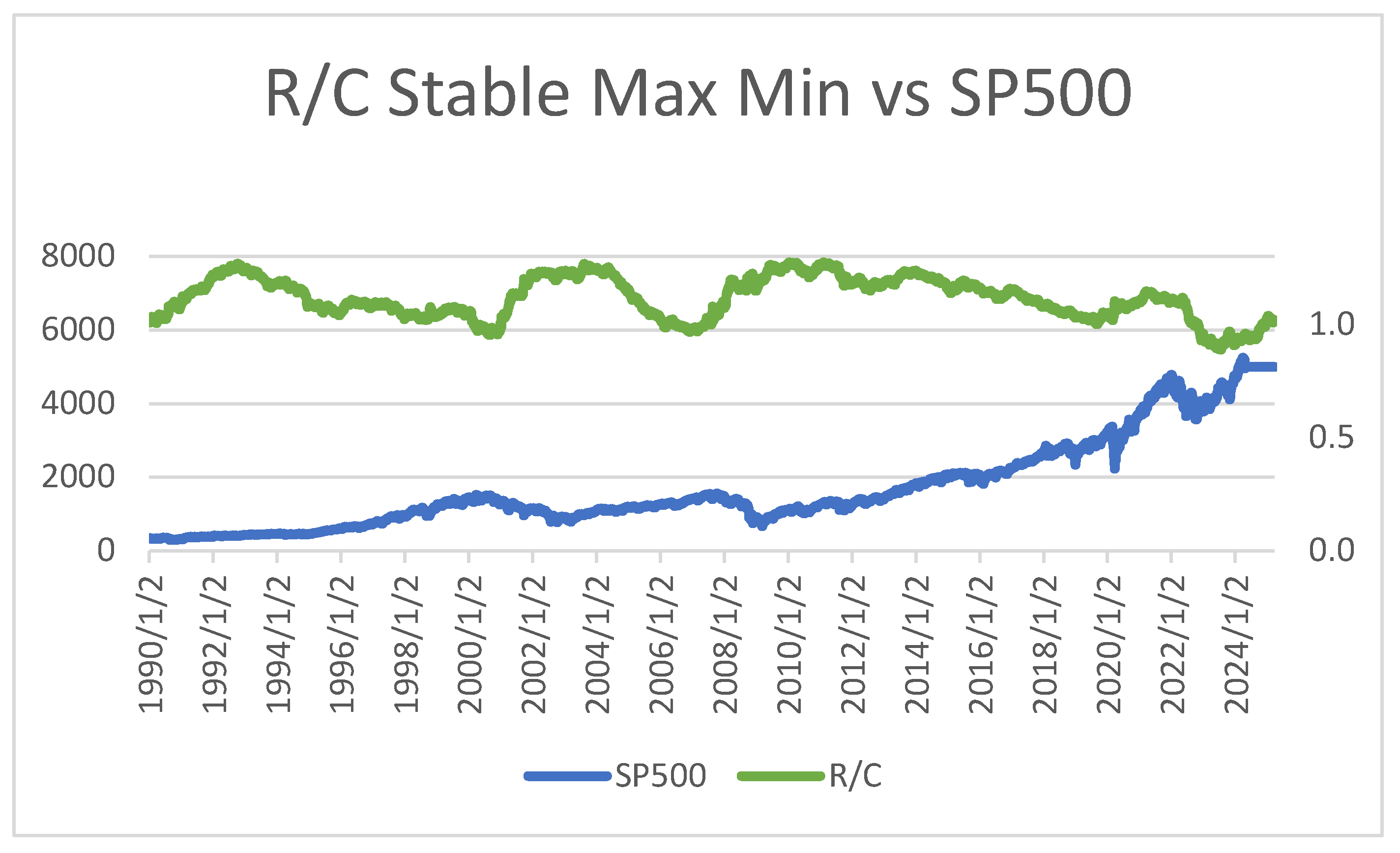
Figure 2.
Relationship Between R and C over a Business Cycle.
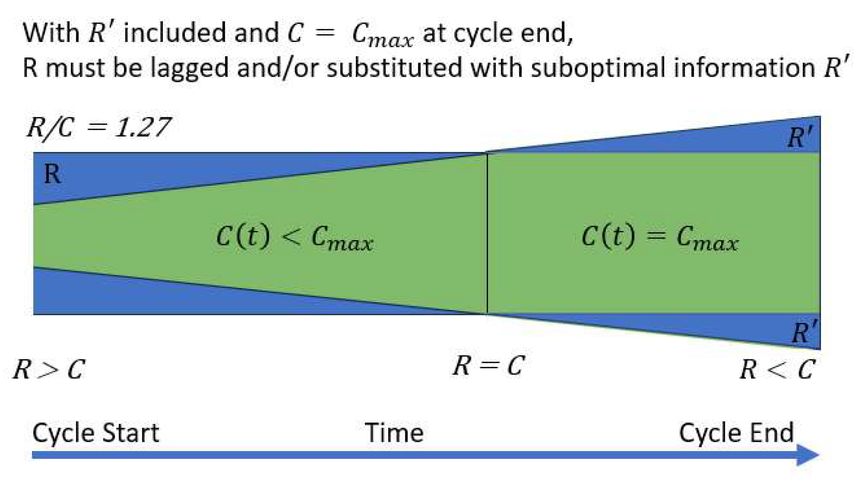
Figure 3.
Fixed Total Maximum Compute (Isocompute) vs Changing Data/Model Size.
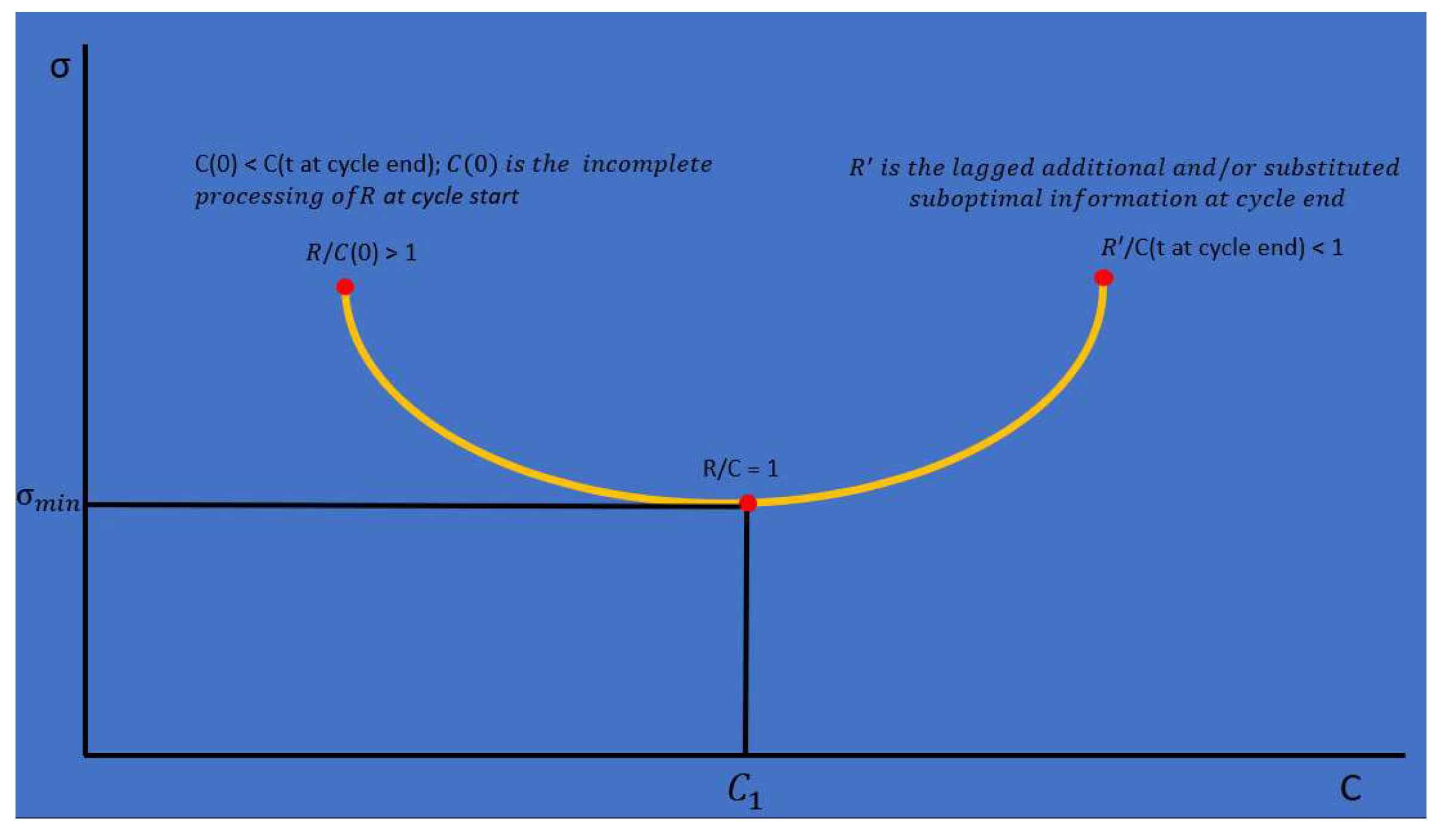
Figure 4.
Variance of R/C 1990-2024.
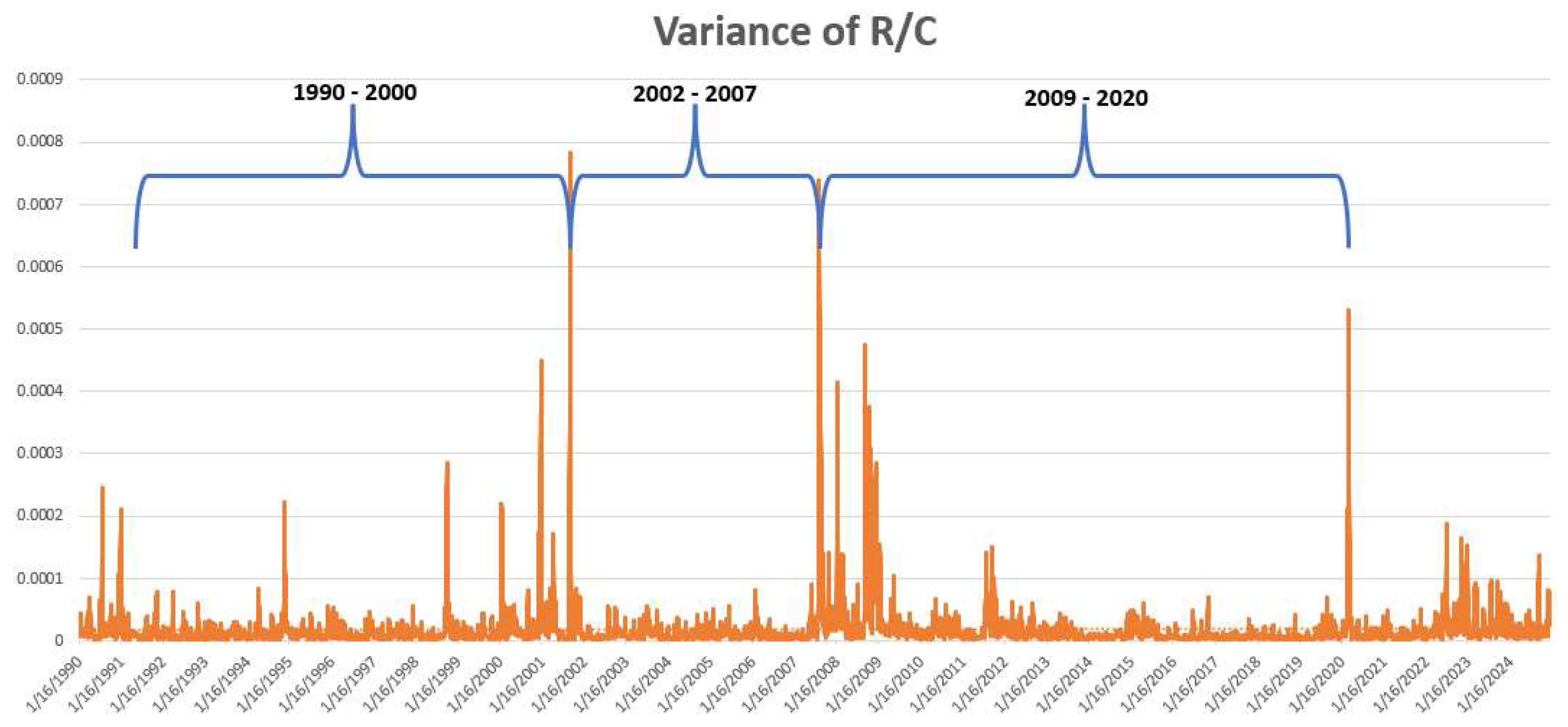
Figure 5.
Explanation of Sigma over last 3 Business Cycles.
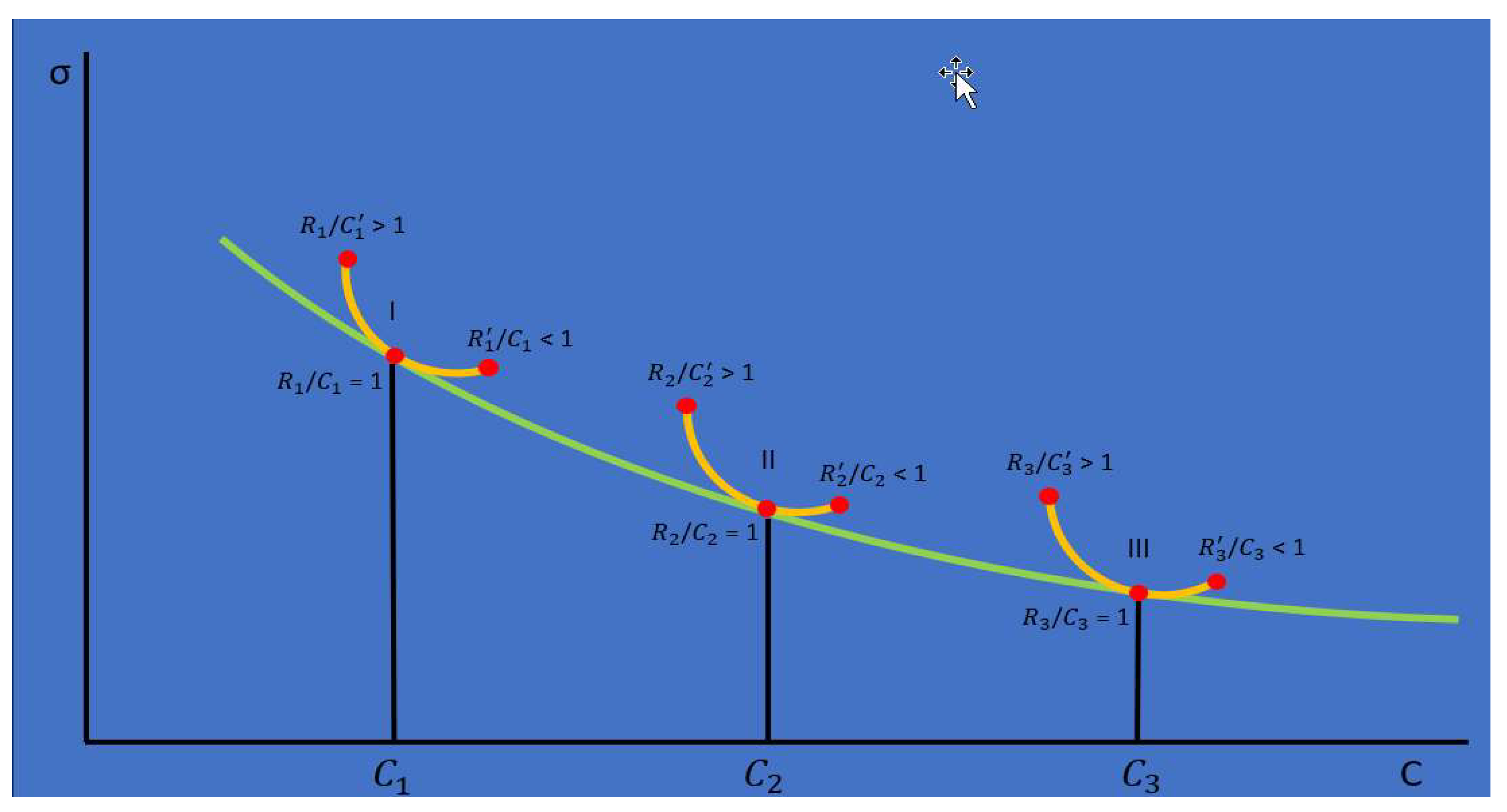
Figure 6.
Empirical Estimation of the US Economy’s Computational Error (Sigma).
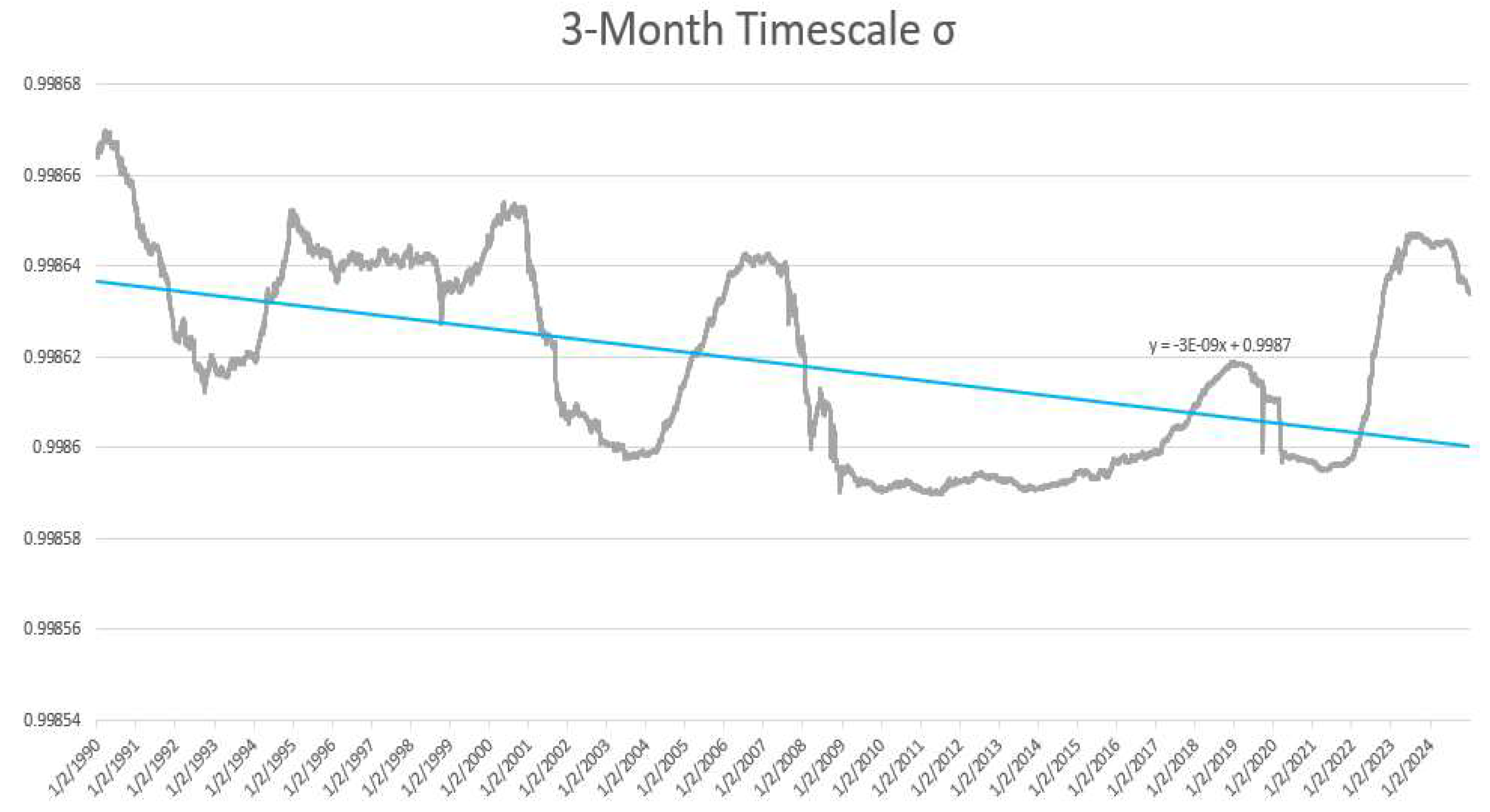
Figure 7.
Positive R/C Shock at Covid Onset March 2020.
| 1 | The 3-month series is the shortest timescale that has values over the entire time period studied. |
Disclaimer/Publisher’s Note: The statements, opinions and data contained in all publications are solely those of the individual author(s) and contributor(s) and not of MDPI and/or the editor(s). MDPI and/or the editor(s) disclaim responsibility for any injury to people or property resulting from any ideas, methods, instructions or products referred to in the content. |
© 2025 by the authors. Licensee MDPI, Basel, Switzerland. This article is an open access article distributed under the terms and conditions of the Creative Commons Attribution (CC BY) license (http://creativecommons.org/licenses/by/4.0/).
Copyright: This open access article is published under a Creative Commons CC BY 4.0 license, which permit the free download, distribution, and reuse, provided that the author and preprint are cited in any reuse.


