
Submitted:
17 April 2025
Posted:
21 April 2025
You are already at the latest version
Abstract
Modern computational models tend to become more and more complex, especially in fields like computational biology, physical modelling, social simulation and others. With the increasing complexity of simulations, modern computational architectures demand efficient parallel execution strategies. This paper proposes a novel approach leveraging the reactive streams paradigm as a general-purpose synchronization protocol for parallel simulation. We introduce a method to construct simulation graphs from predefined transition functions, ensuring modularity and reusability. Additionally, we outline strategies for graph optimization and interactive simulation through push and pull patterns. The resulting computational graph, implemented using reactive streams, offers a scalable framework for parallel computation. Through theoretical analysis and practical implementation, we demonstrate the feasibility of this approach, highlighting its advantages over traditional parallel simulation methods. Finally, we discuss future challenges, including automatic graph construction, fault tolerance, and optimization strategies, as key areas for further research.
Keywords:
parallel simulation
; reactive streams
; logical processors
; transition functions
; state space
; synchronization protocol
1. Introduction
As simulations become increasingly complex, more and more computational resources are required to execute them. Computing power continues to grow per Moore’s law, but this growth shifts to the horizontal plane—i.e., it happens due to an increase in the number of parallel processors and their cores. Thus, there is a need to develop parallel-simulation algorithms capable of utilizing the computing resources of multiple CPUs.
Today several approaches exist for parallelizing simulations. In particular, we can consider the Time Warp algorithm,[1] described in detail in.[2] This algorithm has been studied for many years and has several implementations in the code.[3,4,5] However, Time Warp uses its own synchronization protocol, which is complex and low-level.[6] The RxHLA software framework (based on the reactive adaptation of IEEE 1516 standard)[7] is similar to Time Warp in terms of complexity and low-levelness. Another approach, based on the CQRS + ES architecture, is described in. [8] However, the authors of that work concentrate more on the practical aspects of implementation without much theoretical background. The HPC simulation platform [9] is also a more practical implementation of parallel simulation; it is based on actors and the AKKA library, constituting a more conservative approach than reactive streams.
The key concept of this paper is to use a general-purpose synchronization protocol to parallelize simulations: namely, the reactive-streams protocol [10,11,12], particularly the version that is implemented in the AKKA library. [13,14,15,16]. Thus, on the one hand, we have a classical mathematical model. On the other hand, we have a general-purpose synchronization protocol. The goal of this work is to unite them.
The rest of this manuscript is organized as follows:
- Section 2 explains the basic modeling concepts and entities that we will use in this paper.
- Section 3 extends basic modeling to be represented in the form of a transition graph and shows how a simulation can be performed on this graph.
- Section 4 shows how the transition graph can be implemented with reactive streams and how simulation can be executed.
2. Substates
Before we start developing a parallel-simulation algorithm with reactive streams, we define substates concepts and some objects for later use in this paper. Before reading this section, we suggest you check Supporting Information Appendix A, which describes notation and Supporting Information Appendix B which give common basic definition used in this article. Also, in the Section 5 and Supporting Information Appendix F you can find real word examples which illustrate the described approach.
2.1. Substates as a Decomposition of the State
Each state can be represented as a set of substates, each of which contains only a part of the values of . There must be a way to determine which of the substates belongs to a certain . One option to achieve this is to use a unique key to mark all substates belonging to a certain
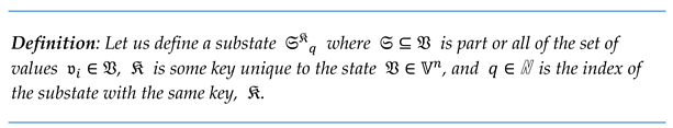 |
One or more values can be used as key . In this case, it makes no sense to include them in any of the substates, since they will be presented in the key.
For some state , we have the set of substates with the same key . We will denote this set by a bold . With such representation of the state , it is necessary to ensure that all marked by the same are not contradictory. The pair of with the same key can be contradictory if one or more values differ under the same index.
 |
In this paper, we will talk about arbitrary sets of substates , the only requirement for which is to meet the consistency criterion.
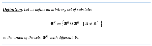 |
Notice that these definitions do not require the presence in the set (and consequently in ) of a sufficient number of substates to cover all values .
Let us also note that, by definition, the set can contain more than one substate with the same key . However, on an arbitrary set that contains duplicate keys , we can construct a set that does not contain them. For this, we need to combine all substates with the same key into one substate:
where is a set with duplicate keys and is a set with unique . Thus, we can say that an arbitrary set of substates can be considered as a key-value structure or as the surjective function
As follows from the definition, the set can only be constructed from a set of states in which a unique key can be associated with each state . Otherwise, this will lead to the appearance of substates in conflict.
The inverse transformation, i.e., the construction of from an arbitrary
is possible only if contains enough substates to construct each state completely.
The set of substates can be equivalent to the state space if this state-space contains enough substates to construct each state . We will denote such a set by .
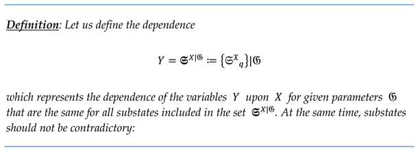
2.2. Representation of the Dependence of Y on X as a Set of Substates:
The dependence of the variables upon can be represented as a set of states . This representation is an alternative to a set of functions. In this case, it is convenient to choose the values as the key and the subset of the values as the values of (including ).
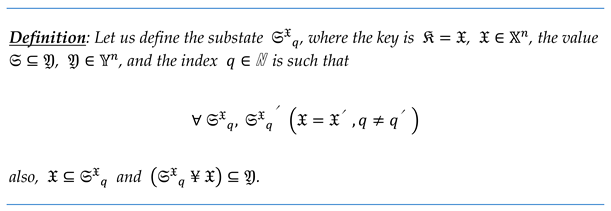 |
Since the values of the parameters are constant for any possible values of and , they are also constant for any possible substates composed of the values of and . Thus, the definition of does not include values . Being joined into a set, the substates will have the same parameters , but may have different values of the key .
 |
The set with all substates having the same key will be denoted .
Let us note that we do not impose a completeness restriction upon the set —i.e., may not contain all of the keys or may even be empty: . may also not contain all and/or it may not contain enough to build one or more complete .
The representation is equivalent to the representation if and only if, for each at a given, the representations are equal:
For each key , there exists a set of substates that cover all possible values . We will denote this set by . This set may not satisfy the consistency criterion (formula 1) and will have cardinality
If we join the sets for all possible keys , we obtain the set of all possible substates. We will denote it by
The cardinality of this set when will be
Moreover, since, from the set only, one set of values is used (note, the cardinalities will be equal in case ).
In practice, we will more often see sparse , where it is impossible to completely construct for every . The use of sparse will reduce the modeling accuracy. In general, this is not a problem from an engineering standpoint since increasing or decreasing the cardinality allows us to choose an acceptable accuracy level for solving a specific simulation problem.
2.3. Reflection as a Record of Changes in the Values of Variables
We can reflect the behavior of a modeled object by measuring its properties and recording the corresponding values of the variables , and . By abstracting from a specific implementation, we will call such a record a reflection of the modeled object.
 |
We can graphically represent the building of the reflection by adding the points
into the state space at the coordinates , where , , and . The added points will form a geometric figure that reflects the behavior of the modeled object.
A reflection can be represented as a set of functions
or as a set of states
In the first case, a set of functions can be constructed by recording the obtained or measured values of the variables , and . [17] In the second case, from the values of obtained or measured with respect to and , the substate can be directly built and added to the set of substates .
In this case, writing down the values of the stopwatch (which reflects the variable ) and the level gauge (which reflects ), we obtain the function , which reflects the dependence of on . In practice, this function will be defined only on a certain interval or several intervals of the time , during which the measurement was performed.
2.4. Model as an Imitation of Changes in the Variables V
In one of several ways, we can define the dependences of the variables on and without directly measuring the properties of the modeled object [18,19,20]. We will call the dependence defined in this way the model of the modeled object.
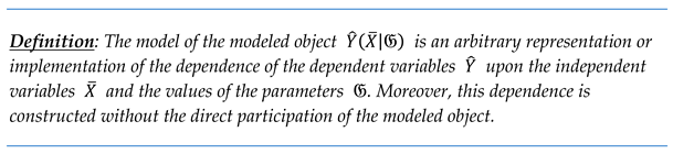 |
We can graphically represent the model as a geometrical figure in the state space consisting of the points
that define the relationship between the variables and and the parameters , where , and .
The model can be implemented as a set of possibly partial functions
or as a set of states
In the first case, the set of functions can be determined analytically or in another way. In the second case, many substates must be pre-built in one way or another.
We can define the model such that it completely coincides with certain reflection ; however, it is much more reasonable and useful to construct to predict changes in the modeled object.
From a practical point of view, we are interested in how accurately the constructed model corresponds to the modeled object. One way to determine compliance is to compare the model and reflection (i.e., to calculate the magnitude of their inconsistency in one way or another). Let us denote the inconsistency value by .
For example, for the case in which all variables have domain , we can define as the integral sum of the difference of the values and for each :
where .
2.5. Simulation of the Model as a Calculation of a Subset of from the Subset and the Parameters
The simulation task can be reduced to obtaining or calculating the subset of the unknown values of the dependent variables from the subset of the known values of the independent variables and the values of the parameters using a certain model .
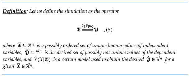 |
For the case where the model is implemented as a set of functions (formula 3), the simulation
is simply a calculation of the result for each argument :
Where
which is the operation for calculating for a given . For a model implemented as a set of substates (formula 4), the simulation is a matter of finding all substates for each key and then building the values of from the found substates
Where
is the operation for selecting a subset of substates with the same key .
A simulation can be interactive—i.e., it can react with external events and produce the results to the outside right during the calculation. In the simplest case, an interactive simulation can be represented as a series of simulations
of the set of models
for the corresponding sets of subsets of values of independent variables sequentially received during the interaction and the sets of dependent sequentially returned as simulation results.
3. Graph Modeling
We show how the model can be represented as a transition graph and how a simulation can be performed for this representation. We define and prove the rules for constructing a consistent transition graph. Before reading this section, we recommend to check Supporting Information Appendix C, which describes transition function concepts. In Section 5 and Supporting Information Appendix G, we present a simple example of the construction and simulation of a transition graph.
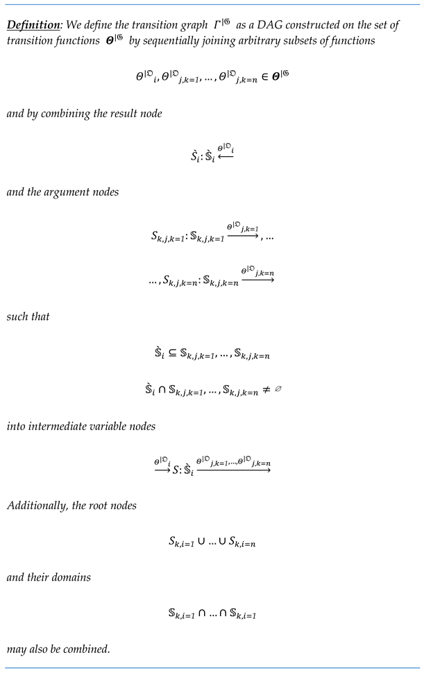
3.1. The Transition Graph and the Simulation Graph
We can join function and a set of functions represented as graphs by combining the result nodes
and the argument nodes
with intermediate-variable nodes
(see Figure 1).
We continue in the same way to sequentially join the functions included in the same set (possibly using the same function more than once); we obtain some DAG (see Figure 2). We call such DAG a transition graph. Also, optionally we can combine two or more root variables that do not have incoming edges, thereby reducing the total number of nodes.
 |
We note that this definition imposes no restrictions on the graph structure except for its acyclicity (the result of the next joined cannot be connected with the argument of any already joined ) and continuity (all nodes of the graph are connected by at least one edge).
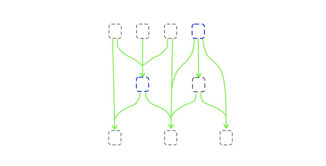
When we join the transition functions , we also join the transitions from the equivalent set , forming a set of more complex DAGs with the same structure as the graph , but which consist of the substates and transitions (see Figure 3). We call such DAGs simulation graphs.
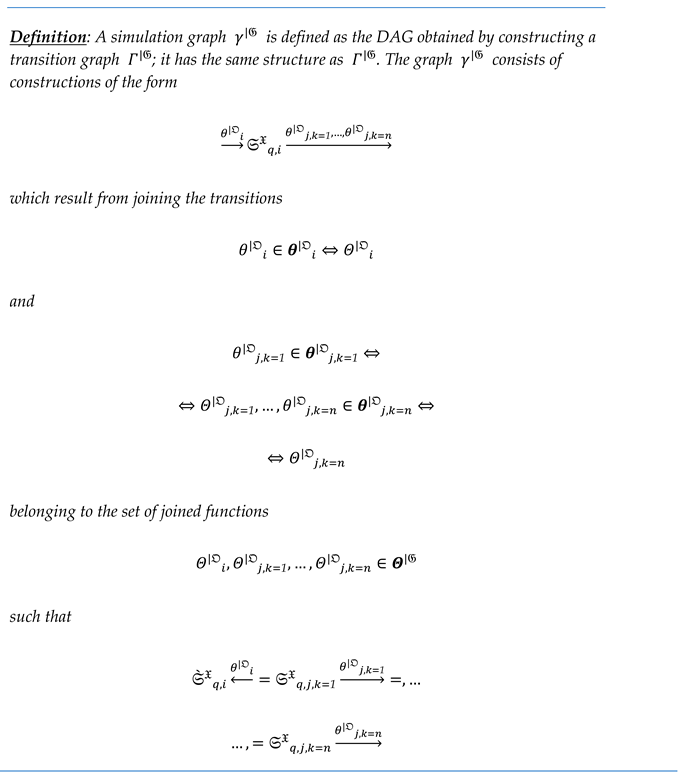 |
We note that all will have a structure exactly matching . According to the definition of , during the construction of , incomplete graphs of with structures not coinciding with that of will be discarded. Thus, the substates included in the discarded graphs will also be removed from the domains of the variables included in the constructed .
Let us denote some arbitrary set of graphs by . According to the definitions of the graphs and , each of the substates from the domains of the variable nodes will belong to one of the simulation graphs . All terms that do not belong to any will be discarded during the construction of , along with the incomplete .
Thus, we can represent the graph as an equivalent set of graphs . We will denote such a set as ; this set will include all from all domains :
where is the set of domains of the variable nodes from the graph and is the set of all belonging to , which is consistent:
Moreover, all simulation graphs will share the same set of parameters split into parts .
Let us index each node from the set with the depth index
where , is the set of all possible paths from any root node (i.e., the node that has no incoming edges) to the indexed node and is the length of the path (the number of edges in the path). Let us also index all transition functions with the same index same as the index of the result node
Thus, each root node of will have and each leaf node (i.e., such that it has no outgoing edges) will have , where is the minimum number of edges to the nearest root node .
3.2. Construction of a Consistent Transition Graph
From a practical viewpoint, we want to be able to construct transitions from a set of predefined transition functions —in other words, to build models from a set of ready-made functional blocks, similar to the Simulink software. It is necessary to guarantee the consistency of at the local level, i.e., at the level of individual functions , to implement this approach successfully.
We can represent some simulation graph as the set of directional paths (dipaths) covering all substates and transitions .
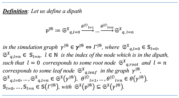 |
We denote some arbitrary set of paths by , which is not necessarily related to the same graph .
The set of paths can be equivalent to the graph if the paths in this set contain all substates and transitions :
In order to guarantee the consistency condition
for the graph (i.e., to guarantee that each of the simulation graphs described by will not contain any inconsistent substates), the graph must meet the following two restrictions:
- For each graph, each substate(i.e., located on one of all possible paths) must have a unique keyregarding the.
- For each graph, the valuesof some variableshould only belong to the set of substatessuch that there exists inat least one path,including all of these substates.
At the local level (i.e., without studying the entire graph ), the above restrictions can be met by applying the following construction principles (Supporting Information Appendix D):
- I.
- The set of keysmust be linearly ordered;
- II.
-
Each transition function(where ) for each transition(where ) in some graph must generate the resulting substate such that its key will always satisfy the conditionsorwhere
- III.
-
For each variable, its valuesmust belong to no more than one root node:where(i.e., the set of all values in all substates form the domain of the variable ).
- IV.
-
If, for some node and some variablethe conditionis true, then, either the node must be a root, or there must be a transition functionwith one or more argumentsfor which the conditionis true and in the graphthere exists a chainthat includes all. Moreover, for the last argumentin the chain, there should not be another functionfor which the conditionis true.
In practice, principle (I) can be easily implemented since linearly ordered sets are common. For example, time, speed, etc., can be represented using variables with ℝ. Next, if the domains of all independent variables are in linear order, then the set of keys will also be in linear order.
Principle (II) says that the key-value constantly increases or decreases as the simulation graph is calculated. This approach can be applied, for example, to physical models, where independent variables are usually rational numbers that increase or decrease over the simulation.
Principle (III) holds if the graph has a single root node such that in each graph there will be only one substate thereby excluding the possibility that the values of the same variable are in different substates .
Another approach to implementing (III) is for each root node to include values only from its own unique set of variables , such that
This approach, for example, is convenient in the graphs used for interactive simulation, where each next node reflects the next input of data from outside the simulation.
In practice, a simple way to implement principle (IV) is to check whether adding the next function to form does not include variables that are already in the results of the functions that have joint arguments with . For example, if there are nodes and for which and , where
and these nodes are the arguments of some function
for which the result is , then we can add only a function
for which and either or , but not .
3.3. Computability of the Simulation Graph and the Initial Set of Substates
In practice, we will need to find some specific simulation graph from some known set of consistent substates associated with the nodes of the graph . We will call the initial set of substates.
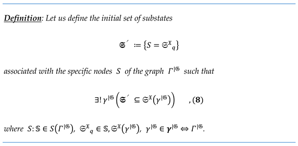 |
The search for a specific graph with some set can be imperatively represented as a calculation of all functions using as the initial arguments for these functions.
Note that the definition requires that be a subset of the one and only one set . However, in the general case, some can be a subset of more than one . In this case, in the imperative representation of the search, a single graph cannot be calculated from such , since for some or all functions , not all arguments be defined.
Representing the search for a specific in the form of a calculation of the functions , we notice that all will be calculated only if the values of all root nodes are known or can be obtained in some way. Thus, is a subset of the unique set (formula 8) if and only if, for each initial node , there exists a path
where is a node whose value is defined in . And all function on this reversible (Supporting Information Appendix E).
3.4. Representation of the Dependence of Y on X in the Form of a Simulation Graph and a Graph Model
The dependence of the dependent variables upon the independent variables can be represented as a tuple of the transition graph , and the set of initial substates with given values of the parameters .
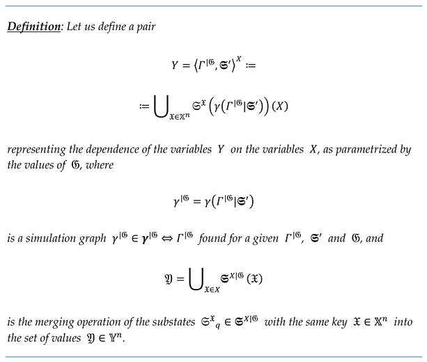 |
The representation can be used to implement the model ; we call this implementation a graph model and denote it as
This implementation is similar to a representation in the form of a set of substates (formula 4), except that the set must first be found as
3.5. Simulation of the Graph Model as a Calculation of a Subset of the Values on the Subset and the Parameters G
For the graph model , we can define the simulation as the operator
where is the subset of known values of the set of independent variables and is the subset of unknown values of dependent variables .
The simulation can be implemented as a search for the simulation graph for a given initial set and a set . Then, from the set is constructed for each as:
In the simulation problem, we can significantly optimize the search for the graph . Since the set is usually much smaller than , we can search or calculate only a part of the substates from , which contain all the required keys :
We can also optimize by including substates that are as close as possible (from the point of view of the distance in graph ) to substates from the desired or even equivalent to these substates. This will reduce the number of calculations not related to the search for (see Figure 4).
For the graphical model , an interactive simulation can also be performed. In the simplest case, this requires many models ; however, a more interesting and optimal approach is to undertake interactive manipulation of the values of the nodes when imperative representations (sequential calculation of the functions ) of the operation are used. This approach was explored briefly in. [23]
Two patterns are possible here:
-
Push pattern:This pattern can help synchronize the simulation with some external processes (for example, to synchronize with real-time). The essence of the pattern is that some functioncannot be calculated until all its argumentsare defined; thus, we can locally pause the simulation, leaving some of the root nodesuninitialized. We can then continue it by defining these nodes.
-
Pool pattern:This pattern can be used to implement an asynchronous simulation reaction to some external events—for example, to respond to user input. As in the previous case, someremain uninitialized. However, the simulation does not stop there. Their values are constructed as needed to calculate the next. Using this approach, it is figuratively possible to imagine that undefinedis computed by some set of unknown transition functions, possibly also combined into a transition graph. In other words, there is some “shadow” or “unknown” part of the graphand, as a result of its calculation, theis initialized (seeFigure 5).
4. Logical Processors
We show how the graph model can be implemented using the reactive-streams paradigm in the form of a computational graph. We also show how the simulation can be evaluated on this graph and offer ways to optimize it. Additionally, in Supporting Information Appendix H, we implement a simple computational graph and perform a simulation with it.
4.1. Reactive Streams and Graph Model
The concept of reactive streams was formulated in 2014 in manifest [10,11,12] and extended by AKKA library developers with tools for composing reactive streams into computational graphs, [13,24] which are already widely used in practice. [9,25,26,27] The graph nodes are logical processors, and the edges are the channels representing the stream of messages that transmit data; each of the processors transforms the messages in some way. Generally, reactive streams are an implementation of the well-known dataflow-programming paradigm.[25]
This chapter will follow the approach described in (i.e., we will compose a computational system from small blocks that process data streams) [22,28,29]. However, we will use reactive streams to do all the hard work for us to distribute computation and load balancing.
We will denote messages (values) by , logical processors (reactors) by , channels connecting the processors by , and the numeral graph by .
We can transform an arbitrary graphical model (formula 9) into a computational graph :
- To represent each substatewith the message.
-
To replace allfor whichwith equivalent processors:and all(for which) with processorsequivalent to the inverse functions:
- To successively replace all functionsand all argumentsthat are already replaced by the channels, which are equivalent to:
- And to successively replace all, the resultof which has already been replaced by channel, bythat equivalent to the inverse functions:
As a result, we obtain a graph containing the equivalent for each but possibly differing structures compared to , since its construction was carried out starting from rather than from the root nodes (see Figure 6).
Next, each root channel must be connected with a logical processor , whose task is to send the corresponding (where , which starts the computational process (see Figure 7).
Moreover, all or part of the channels must be connected with one or more , which will collect part or all of the calculated substates belonging to the graph given by the set of initial states (see Figure 7).
4.2. Graph Optimization
Simply replacing functions with processors yields an extremely suboptimal and potentially infinite processing graph , which is not good from the viewpoint of minimizing computing resources. To solve this problem, we can optimize graph . For example, consider two optimization methods:
-
Folding of cyclic sequences in the graph:Consider a chain with an arbitrary length of the same functions, as inFigure 8.a. This can be transformed into a chain of logical processorsof equal length, as inFigure 8.b. We can fold this chain into a singleby adding a message-return loop as inFigure 8.c. Thus, more than one messagewill go through one, so that ifhas more than one argument, it can lead to collisions. To resolve collisions and also to implement breakage of the loop, we need to determine the loop-iteration number of messages. The simple way to do this is to add an iteration counter for each loop in. Another approach is to use history-sensitive values.[21] As a more complex example, we consider the graphinFigure 9.a, which can be converted and collapsed into a compact graphas inFigure 9.b.
-
Folding of graph:
In general, the optimization problem for graph is rather complex and goes beyond the scope of this article.
4.3. Simulation of the Graph Model Using the Computational Graph
In the simplest case, we can simulate the model (formula 10) using the graph constructed on it in two stages:
-
Calculate the set of substatesFor this, we initialize the calculation by sendingmessages using the processors. Using the processors, we collect all the calculated messages,.
- Find all substates for each keyand then collect the valuesfrom the found substates (formula 6).
In most cases, this approach will be computationally expensive, since in practice, usually .
Generally, simulation optimization is the minimization of the number of calculated substates such that . Several approaches are possible here—for example, constructing a minimalistic with a certain well-known collection . Alternatively, lazy algorithms that cut off the calculations whose result is not required to cover could be used. However, this topic is beyond the scope of the present article.
5. Practice
In this chapter we show our approach in practice. First, we describe modeled object, then define it mathematical model and the analytical solution. In the next step, explain the procedure of construction of graph and parallelization scheme and present the results. This chapter contains shortened description, please check Supporting Information Appendix F, G and H for the full one.
5.1. Description of the Modeled Object and the Construction of Model
As an example, consider the classic model of saline mixing. Here, the simulated object is a system of two connected tanks of volumes and . Over time , a saline solution circulates from the first tank to the second with a speed and in the opposite direction with a speed of . In addition, the saline solution is poured into the first tank at a speed of and drains from the second tank at the same speed , i.e., the volume of the saline solution in the tanks does not change. Initially, the first and second tanks are entirely filled with solutions with initial salt concentrations of and , respectively. A saline solution with a concentration of is supplied to the first tank constantly. Thus, the set of variables reflecting the properties of interest will look like:
The modeling task is to predict the change in the salt concentrations and over time .
As part of the modeling problem to be solved, we represent the simulated object in the form of the model (formula 3), breaking the variables as
and specifying their dependence as a set of functions:
Which are obtained by solving of the Cauchy problem
We can also represent the simulated object in the form of model (formula 4). In this case, the values of the variable will be used as keys and those of the variables and can be separated by different substates, such that we obtain two types of substates and . In the code, we can represent the values , and the substate as OOP classes (source code B.1.L27).
One simple, but impractical, way to construct a set of substates is to generate using a set of functions (formula 12) with some step of key (source code B.2.L60).
Using the model we can perform the simulation (formula 5) for some segment and obtain the corresponding set of values (source code B.1.L71 is an implementation of and the source code B.2.L70 is an implementation of ). Looking at the output plots, we can see that they are similar (see Figure 10).
We can compare the results of executing of models and just by accumulating different overall output values:
Evaluating this algorithm (source B.3.L24), we obtain .
5.2. Building and Simulating a Graphical Model
The graph for this example will represent an infinite chain of pairs of nodes connected by edges . For convenience, in addition to the index of depth , we to index the nodes with indices of width , such that the nodes with the same index will have different values of . Moreover, we set , where is the index of the argument (edges) and q is the index of the substate assigned to . Each pair and corresponds to a certain moment of discrete-time . For simplicity, we will use a fixed time-step , where is the depth index and is the time-step coefficient. Also, we restrict model time to a small interval . In this case, the graph will contain
pairs of nodes .
The simplest way to implement the transition functions and is to use the functions and from the set (formula 13). In this case,
A slightly more complicated implementation is to rewrite the system of differential equations (formula 14) to be solved by the Euler method
as iterated by :
In this case
We implement the nodes and the sets of edges as OOP classes (source code C.1.L89). nodes are essentially variables that are not initially defined. The transition graph and the simulation graph can be represented as classes containing collections of nodes of sets of edges (source code C.1.L149). Moreover, the graph is the same as graph , but with all variables defined.
Due to the simplicity of the transition graph , we can implement the function build_Γ(, ), which automatically constructs based on the given number of steps and the time-step (source code C.1.L190).
The search for the simulation graph is a calculation of the values of all nodes from the initial set of substates
We implement the search as method .γ(), using the indices and as the key in the set (source code C.1.L156). The method first initializes the nodes and with the initial substates and and then calculates the values of the rest nodes by calling each method .eval() until all are defined. The method .eval() checks whether the arguments
are defined and, if so, evaluates the result
The set of substates can be obtained from the simulation graph by simply extracting the values from the nodes and combining them into the set . We implement this in the form of the method .() (source code C.1.L179); next, can be used to obtain the values of from the values of .
5.3. Constructing and Calculating Graph Using the Graphical Model
As an example, we construct graph using the model for mixing salt solutions. To implement it, we use the AKKA Streams library. There was a similar approach to implement the SwiftVis tool.
We can build an unoptimized version of graph by simply replacing the functions and with logical processors and and adding , , and .
We represent the substates in the form of the messages produced by the corresponding , where . In particular, the substates from the set can be represented as and .
This will work as follows (see source code D.1): the initial messages and are sent by logical processors and to the processors , . Then, the messages will distribute throughout the graph, where a copy of each substate is fed into the processor , which builds the resulting set of substates .
Since the standard blocks Zip, Flow.map, Broadcast, and Merge from the AKKA Streams library were used to construct graph , the implementation of each will be a nested graph.
Since the obtained graph consists of recurring pairs and , it can be optimized by implementing two cycles using 2 logical processors and .
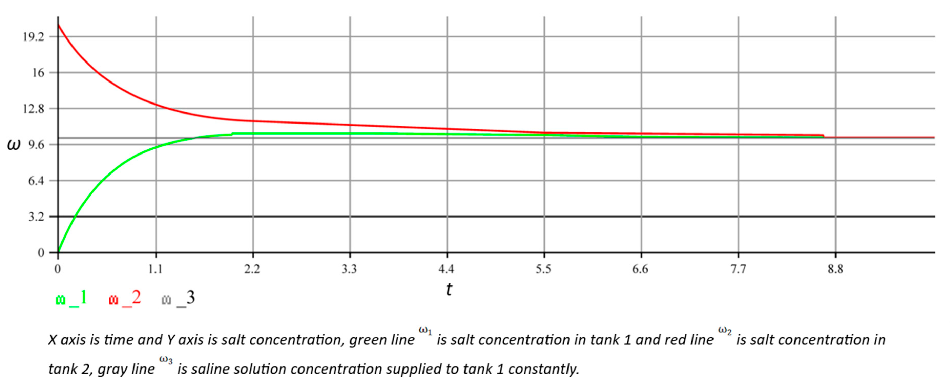
Since it is necessary in this case to determine which incoming messages refer to particular iterations of the cycle, we add the iteration (depth) counter to them, , and modify the grouping function Zip so that it selects pairs of incoming with the same value (source code D.2). When we execute this code, we obtain the simulation result (see Figure 11), which was the same as our findings from the implementation of the model (see Figure 10).
6. Discussion
One of the primary contributions of this research is the synthesis of classical mathematical modeling techniques with the practical, high-performance synchronization mechanisms provided by reactive streams. Similar to earlier approaches such as the Time Warp algorithm[1,2] and actor-based frameworks used in HPC simulation platforms[9], our method decomposes the complete object state into substates with unique keys. This modular representation not only supports reuse and flexibility but also enables the direct mapping of transition functions to logical processors. The resulting computational graph is reminiscent of systems such as RxHLA[7] and CQRS + ES architectures[8], which emphasize decoupling and distributed processing.
Representing the model as a transition graph and initial set of sates offers several benefits:
- Modularity and Reusability: By encapsulating transition rules as independent functional blocks, the approach supports reuse and flexibility. This modular structure is similar in spirit to block-diagram environments like Simulink [30,31,32] and has parallels in dataflow programming models discussed by Kuraj and Solar-Lezama [21].
In summary, the proposed method of using reactive streams as a synchronization protocol for parallel simulation provides a compelling framework that unites rigorous mathematical modeling with practical, scalable implementation techniques. While challenges remain—particularly in optimization, continuous simulation, and fault tolerance, the initial results and conceptual clarity offer a solid foundation for further research and development. The integration of our approach with similar studies in the field [1,2,3,4,5,6,7,8,9,10,13,21,22,23,24,25,26,27,28,33,34] highlights its potential and provides clear directions for future work.
7. Future Work
Many unanswered questions remain, some of which we present for future research:
-
Effective optimization of computational graph and simulation on it:Chapters 4.2 and 4.3 dealt with this topic. However, due to its complexity and vastness, it did not fit into this article. In general, this is a very important issue from a practical point of view. Solving it will significantly reduce the number of resources required to perform simulations. Another interesting question is the automation of the optimization of graph . Say that, initially, we have non-optimal , for example, obtained by the method described in Chapter 4.1. We want to automatically make C compact and computationally easy, without loss of accuracy and consistency.To resolve the optimization task the ML technique can be used. For example, reinforcement rearming agents can be trained to explore various graph configurations (i.e., different ways to fold or collapse the computational graph) and learn which configurations yield the best performance in terms of latency, throughput, or resource consumption [36,37,38,39,40]. Also, techniques like neural architecture search (NAS) can be adapted to optimize the layout and parameters of the computational graph. This includes automatically deciding how to fold cyclic sequences, balance load among logical processors, and minimizing redundant computations [39,40,41].
-
Accurate simulation of continuous-valued models:Many properties of modeled objects can be represented in continuous quantities, for example, values from the set ℝ. However, the simulation (the calculation of which is based on message forwarding) is inherently discrete. An open question remains as to how accurately continuous quantities can be calculated. The question is how to increase the accuracy of calculating such quantities without increasing the requirements for computer resources.
-
Fault-tolerance of reactive streams:We did not touch on fault tolerance of simulation in this work, but in most real/practical applications, fault tolerance is very important. This question was partially explored in [23] but we also suggest this for future work.
-
Manual and automatic graph construction :From a practical viewpoint, it is interesting to be able to use some IDE to manually construct a computational graph , and to do this such that the corresponding graph will be consistent and optimal. For example, this might be done similarly to the Simulink package, [30,42] SwiftVis tool, [25,43] or XFRP language [24,44]. It is also interesting to find ways to automate the construction of . For example, the model can initially be defined as a certain set of rules by which graph can be automatically and even dynamically constructed. Specialized programming languages are also an interesting area to explore. For example, the EdgeC [33,35] language can be considered a tool to describe computational graphs.Also, ML technique can be applied wildly here. For example, graph learning techniques from graph neural networks (GNNs) can be applied to learn the structure of the optimal computational graph from historical data. The learned model can then suggest or automatically construct a more efficient graph based on current simulation requirements. Adaptive scheduling ML algorithms can dynamically adjust the scheduling of tasks across logical processors, optimizing the execution order and balancing the load [45,46]. This is particularly useful in interactive or real-time simulations where conditions may change frequently.
-
Testing with complex models and comparing with other parallelizing approaches:This work provides a small, simple example of parallel simulation to show how the described approach can be implemented in practice. However, the questions of checking this approach with large and complex models and comparing its effectiveness with other parallelizing approaches remain open.
Conclusions
The proposed method effectively integrates the reactive streams paradigm with classical mathematical modeling techniques to create a scalable framework for parallel simulation. By using a graph-based representation of object states and transition functions, this approach enhances modularity and reusability while supporting efficient computation through logical processors. The implementation using AKKA reactive streams demonstrates its scalability and practical feasibility for distributed systems. Despite its promise, the work highlights challenges such as graph optimization, continuous model simulation, fault tolerance, and automation of graph construction, which offer significant areas for future research and development. The study lays a strong foundation for advancing parallel simulation techniques, emphasizing both theoretical robustness and practical scalability.
Supplementary Materials
The following supporting information can be downloaded at: Preprints.Org.
Author Contributions
O.S.: Conceptualization, methodology, formal analysis, writing, visualization, software. A.P.: Conceptualization, methodology, formal analysis, writing—original draft preparation, and visualization. I.P.: Methodology, software, formal analysis, data curation, and writing—original draft preparation. M.Y.: Investigation, resources and editing, and visualization. H.K.: Supervision, data curation, and writing—review and editing. V.A.: Supervision, data curation, visualization, and writing—review and editing. All authors have read and agreed to the published version of the manuscript.
Funding
No funding
Data Availability Statement
The raw data supporting the conclusions of this article will be made available by the authors upon request.
Acknowledgments
The research was conducted as part of the projects ‘Development of Methods and Means of Increasing the Efficiency and Resilience of Local Decentralized Electric Power Systems in Ukraine’ and ‘Development of Distributed Energy in the Context of the Ukrainian Electricity Market Using Digitalization Technologies and Systems’, implemented under the state budget program ’Support for Priority Scientific Research and Scientific-Technical (Experimental) Developments of National Importance’ (CPCEL 6541230) at the National Academy of Sciences of Ukraine.
Conflicts of Interest
The authors declare no conflicts of interest.
References
- Jeerson, D. R.; Sowizral, H. A. Fast concurrent simulation using the time warp mechanism, Rand Corp: Santa Monica CA, 1982; Part I: Local Control.
- Richard, R.; M. Fujimoto, Parallel and Distributed Simulation Systems, Wiley: New York, USA, 2000.
- Radhakrishnan, R.; Martin, D. E.; Chetlur, M.; Rao, D. M.; Wilsey, P. A. An Object-Oriented, Time Warp Simulation Kernel. in D. Caromel, R. R. Oldehoeft, and M. Tholburn, editors, In Proc. of the International Symposium on Computing in Object-Oriented Parallel Environments (ISCOPE'98) 1998, 1505, 13-23.
- Jefferson, D.; Beckman, B.; Wieland, F.; Blume, L.; Diloreto, M. Time warp operating system, in Proc. of the eleventh ACM Symposium on Operating systems principles 1987, 21, 77-93.
- Aach, J; Church, G.M. Aligning gene expression time series with time warping algorithms, Bioinformatics 2001, Volume 17, Issue 6, Pages 495–508. [CrossRef]
- Nicol, D.M.; Fujimoto, R.M.; Parallel simulation today, Ann. Oper. Res., 1994, 53, 249. [CrossRef]
- Falcone, A.; Garro, A. Reactive HLA-based distributed simulation systems with rxhla, In 2018 IEEE/ACM 22nd International Symposium on Distributed Simulation and Real Time Applications (DS-RT) 2018, 1-8.
- Debski, A.; Szczepanik, B.; Malawski, M.; Spahr, S. In Search for a scalable & reactive architecture of a cloud application: CQRS and event sourcing case study, IEEE Software (accepted preprint), copyright IEEE(99), 2016.
- Bujas, J.; Dworak, D.; Turek, W.; Byrski, A. High-performance computing framework with desynchronized information propagation for large-scale simulations, J. Comp. Sci. 2019, 32, 70-86. [CrossRef]
- Reactive stream initiative, https://www.reactive-streams.org (accessed on 15 April 2025).
- Davis, A.L. Reactive Streams in Java: Concurrency with RxJava, Reactor, and Akka Streams, Apress, 2018.
- Curasma H.P.; Estrella, J.C. Reactive Software Architectures in IoT: A Literature Review. In Proceedings of the 2023 International Conference on Research in Adaptive and Convergent Systems (RACS '23) 2023, Association for Computing Machinery, New York, NY, USA, Article 25, 1–8. [CrossRef]
- The implementation of reactive streams in AKKA: https://doc.akka.io/docs/akka/current/stream/stream-introduction.html (accessed on 15 April 2025).
- Oeyen, B.; De Koster, J.; De Meuter, W. A Graph-Based Formal Semantics of Reactive Programming from First Principles. In Proceedings of the 24th ACM International Workshop on Formal Techniques for Java-like Programs (FTfJP '22) 2023, Association for Computing Machinery, New York, NY, USA, 18–25. [CrossRef]
- Posa, R. Scala Reactive Programming: Build Scalable, Functional Reactive Microservices with Akka, Play, and Lagom, Packt Publishing: Germany, 2018.
- Baxter, C. Mastering Akka, Packt Publishing: Germany, 2016.
- Nolte, D.D. The tangled tale of phase space, Phys. Today, 2010, 63, 33-38.
- Myshkis, A.D.; Classification of applied mathematical models - the main analytical methods of their investigation, Elements of the Theory of Mathematical Models 2007, 9.
- Briand, L.C.; Wust, J. Modeling development effort in object-oriented systems using design properties. IEEE Transactions on Software Engineering 27.11, 2001, 963-986.
- Briand, L.C.; Daly, J.W.; Wust. J.K. A unified framework for coupling measurement in object-oriented systems., IEEE Transactions on software Engineering 25.1, 1999, 91-121.
- Shibanai, K.; Watanabe, T. Distributed functional reactive programming on actor-based runtime, Proc. of the 8th ACM SIGPLAN International Workshop on Programming Based on Actors, Agents, and Decentralized Control, 2018, 13 – 22.
- Lohstroh, M.; Romeo, I.I.; Goens, A.; Derler, P.; Castrillon, J.; Lee, E.A.; Sangiovanni-Vincentelli, A. Reactors: A deterministic model for composable reactive systems, In Cyber Physical Systems. Model-Based Design, Springer, Cham, 2019, 59-85.
- Mogk, R.; Baumgärtner, L.; Salvaneschi, G.; Freisleben, B.; Mezini, M. Fault-tolerant distributed reactive programming, 32nd European Conference on Object-Oriented Programming (ECOOP 2018) 2018.
- About the graphs in AKKA streams: https://doc.akka.io/docs/akka/2.5/stream/stream-graphs.html (accessed on 15 April 2025).
- Kurima-Blough, Z.; Lewis, M.C.; Lacher, L.; Modern parallelization for a dataflow programming environment, in Proc. of the International Conference on Parallel and Distributed Processing Techniques and Applications (PDPTA), The Steering Committee of the World Congress in Computer Science, Computer Engineering and Applied Computing (WorldComp), 2017, 101-107.
- Kirushanth, S.; Kabaso, B. Designing a cloud-native weigh-in-motion, in 2019 Open Innovations (OI), 2019.
- Prymushko, A.; Puchko, I.; Yaroshynskyi, M.; Sinko, D.; Kravtsov, H.; Artemchuk, V. Efficient State Synchronization in Distributed Electrical Grid Systems Using Conflict-Free Replicated Data Types. IoT 2025, 6, 6. [CrossRef]
- Oeyen, B.; De Koster, J.; De Meuter, W. Reactive Programming without Functions. arXiv 2024, preprint arXiv:2403.02296.
- Babaei, M.; Bagherzadeh, M.; Dingel, J. Efficient reordering and replay of execution traces of distributed reactive systems in the context of model-driven development. Proceedings of the 23rd ACM/IEEE International Conference on Model Driven Engineering Languages and Systems 2020.
- Simulink https://www.mathworks.com/help/simulink/index.html?s_tid=CRUX_lftnav (accessed on 15 April 2025).
- Karris, S.T. Introduction to Simulink with engineering applications. Orchard Publications, 2006.
- Dessaint, L.-A.; Al-Haddad, K.; Le-Huy, H.; Sybille, G.; Brunelle P. A power system simulation tool based on Simulink. IEEE Transactions on Industrial Electronics 1999, 46, 6, 1252-1254.
- Kuraj, I.; Solar-Lezama, A. Aspect-oriented language for reactive distributed applications at the edge, in Proceedings of the Third ACM International Workshop on Edge Systems, Analytics and Networking 2020, (EdgeSys '20). Association for Computing Machinery, New York, NY, USA, 67–72. [CrossRef]
- Babbie, E.R. The practice of social research, Wadsworth Publishing, 2009, ISBN 0-495-59841-0.
- Broekhoff, J. Programming Languages For Programs For Stateful Distributed Systems.
- Zoph, B.; Le, Q. V. Neural Architecture Search with Reinforcement Learning, arXiv 2016, preprint arXiv:1611.01578.
- Nakata, T.; Chen, S.; Saiki, S.; Nakamura M. Enhancing Personalized Service Development with Virtual Agents and Upcycling Techniques. Int J Netw Distrib Comput 2025, 13, 5. [CrossRef]
- Liu, M.; Zhang, L.; Chen, J.; Chen W.-A.; Yang, Z.; Lo, L.J.; Wen, J.; O’Neil, Z. Large language models for building energy applications: Opportunities and challenges. Build. Simul. 2025, 18, 225–234. [CrossRef]
- Kipf, T. N.; Welling, M. Semi-Supervised Classification with Graph Convolutional Networks. International Conference on Learning Representations (ICLR) 2017.
- Nie, M.; Chen, D.; Chen, H.; Wang, D. AutoMTNAS: Automated meta-reinforcement learning on graph tokenization for graph neural architecture search, Knowledge-Based Systems 2025, Volume 310, 113023. [CrossRef]
- Kuş, Z.; Aydin, M.; Kiraz, B. Kiraz, A. Neural Architecture Search for biomedical image classification: A comparative study across data modalities, Artificial Intelligence in Medicine 2025, Volume 160, 103064. [CrossRef]
- Chaturvedi, D.K. Modeling and simulation of systems using MATLAB and Simulink. CRC press, 2017.
- Lewis, M.C.; Lacher, L.L. Swiftvis2: Plotting with spark using scala. International Conference on Data Science (ICDATA’18) 2018, Vol. 1. No. 1.
- Yoshitaka, S.; Watanabe, T. Towards a statically scheduled parallel execution of an FRP language for embedded systems. Proceedings of the 6th ACM SIGPLAN International Workshop on Reactive and Event-Based Languages and Systems 2019, 11 – 20. [CrossRef]
- Bassen, J.; Balaji, B.; Schaarschmidt, M.; Thille, C.; Painter, J.; Zimmaro, D.; Games, A.; Fast, E.; Mitchell, J.C. Reinforcement learning for the adaptive scheduling of educational activities. Proceedings of the 2020 CHI conference on human factors in computing systems 2020, CHI '20: Proceedings of the 2020 CHI Conference on Human Factors in Computing Systems, 1 – 12. [CrossRef]
- Long, L.N.B.; You, S.-S.; Cuong, T.N.; Kim, H.-S. Optimizing quay crane scheduling using deep reinforcement learning with hybrid metaheuristic algorithm, Engineering Applications of Artificial Intelligence 2025, Volume 143,110021. [CrossRef]
Figure 1.
Joining of function
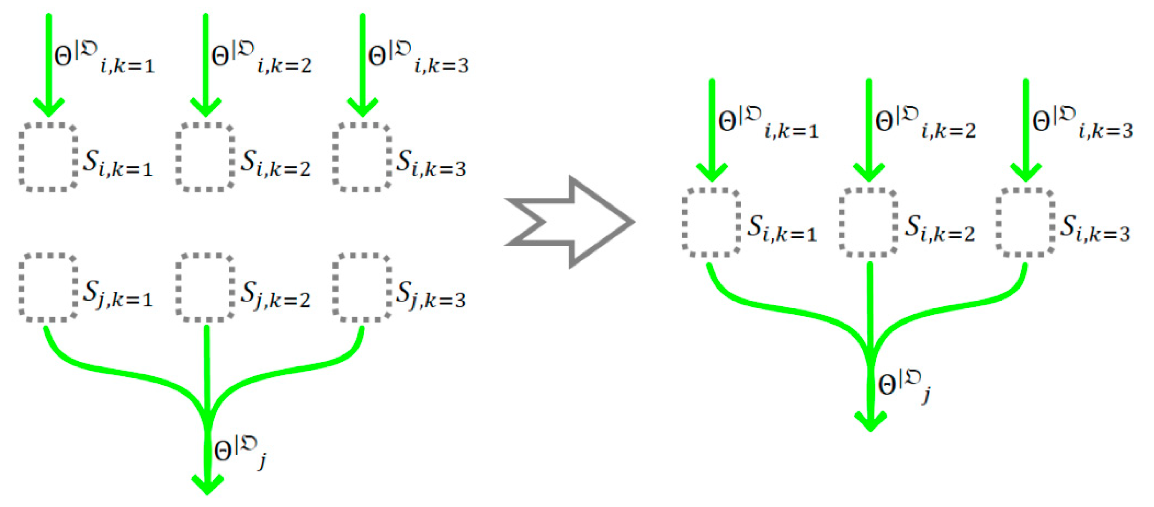
Figure 2.
Example of the transition DAG built from functions
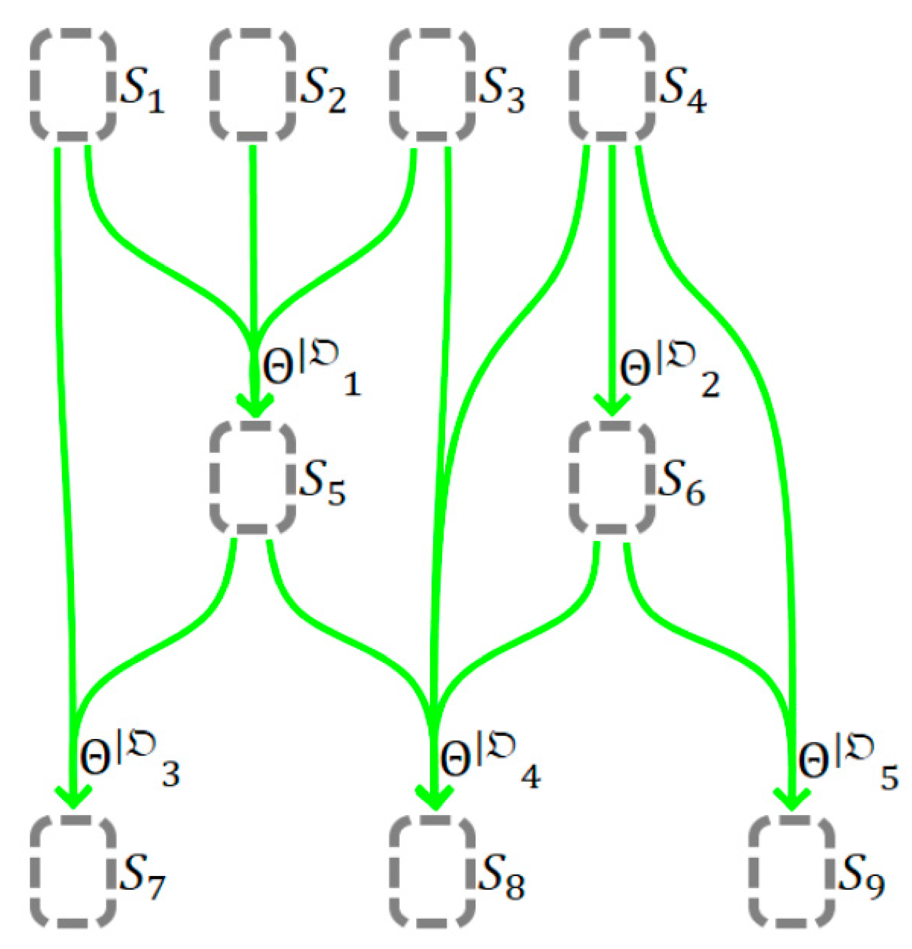
Figure 3.
Example of the simulation graph that can be obtained from the transition graph in Figure 2.
Figure 3.
Example of the simulation graph that can be obtained from the transition graph in Figure 2.
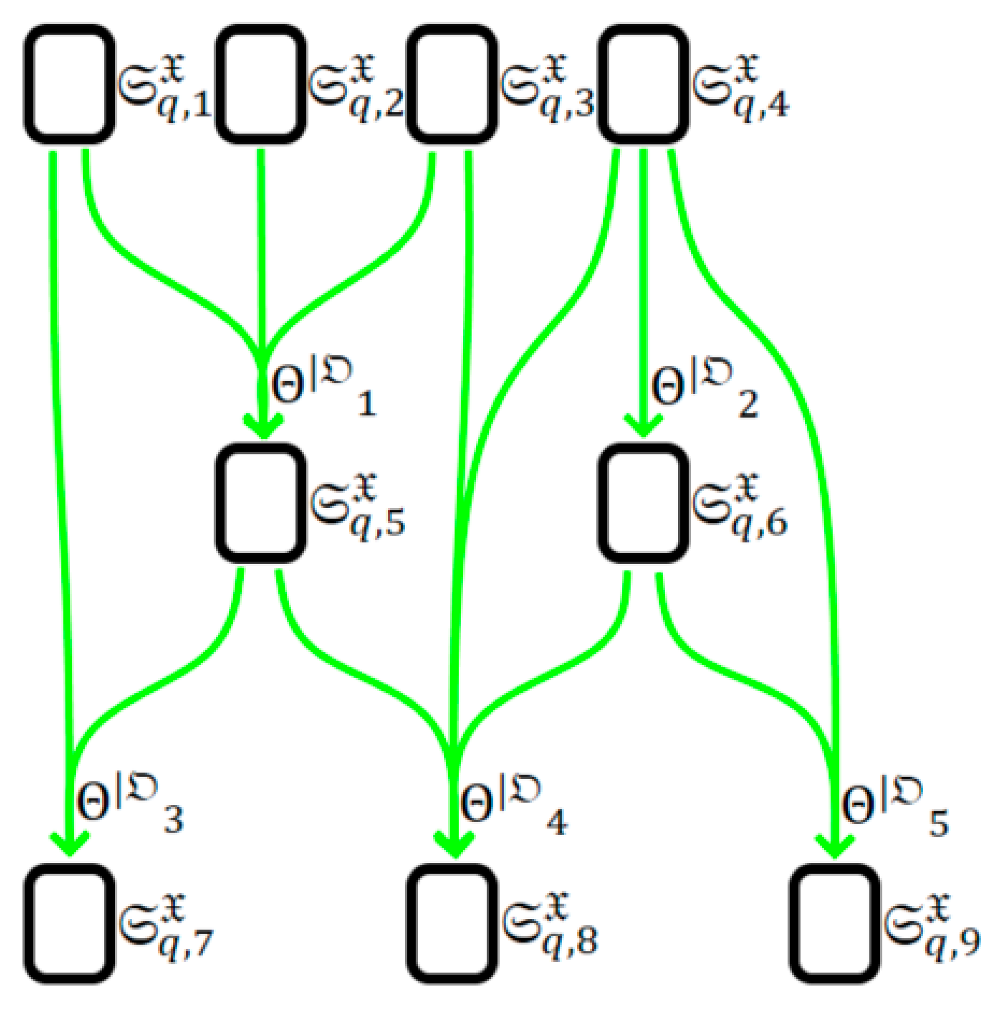
Figure 4.
Reduction of the number of calculations by including substates that are as close as possible to those from the desired
Figure 4.
Reduction of the number of calculations by including substates that are as close as possible to those from the desired
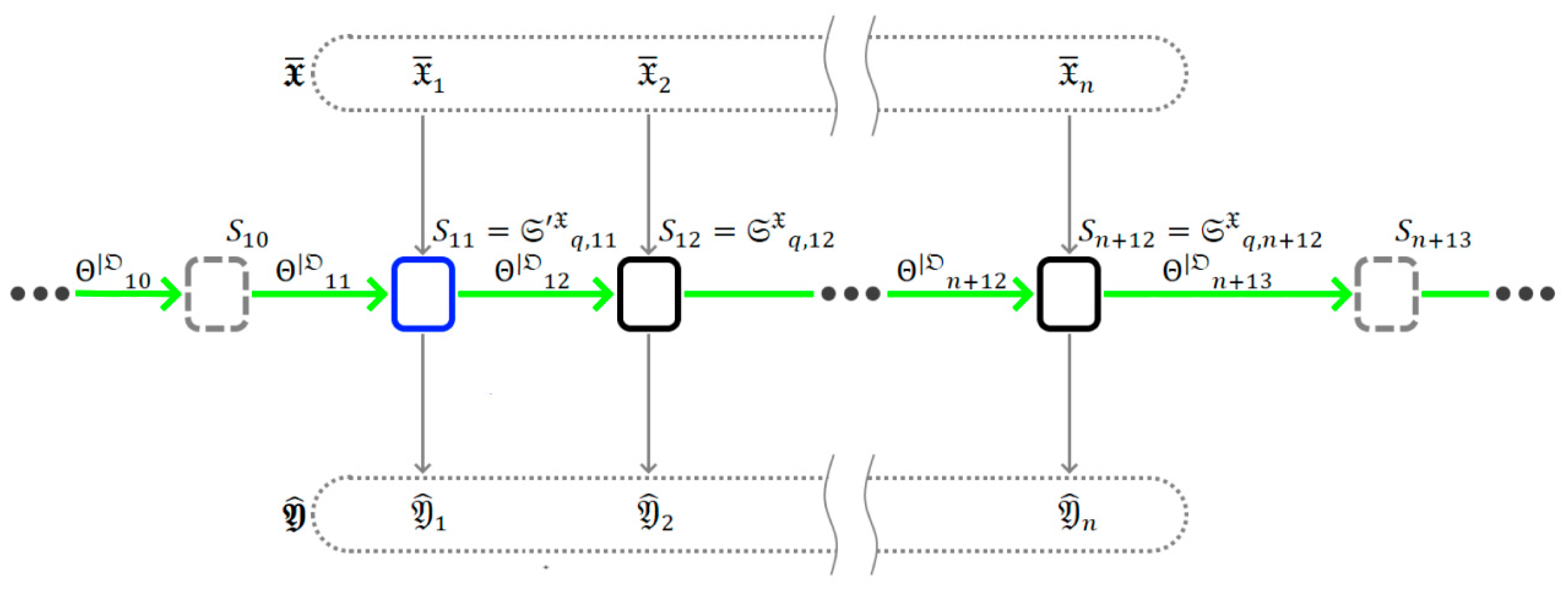
Figure 5.
Representing the input/output as a set of unknown transition functions.
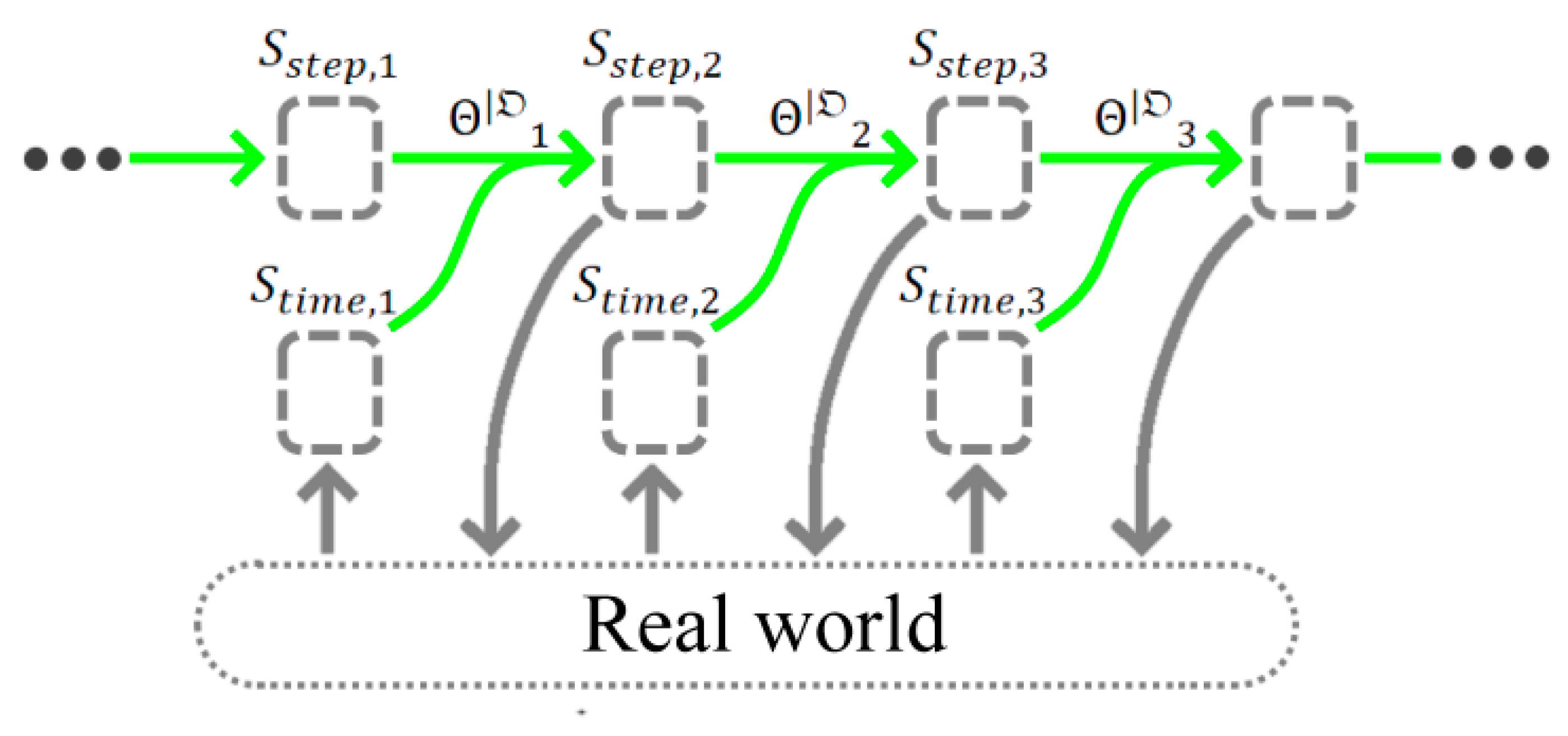
Figure 6.
Example of constructing of the computational graph from the model .
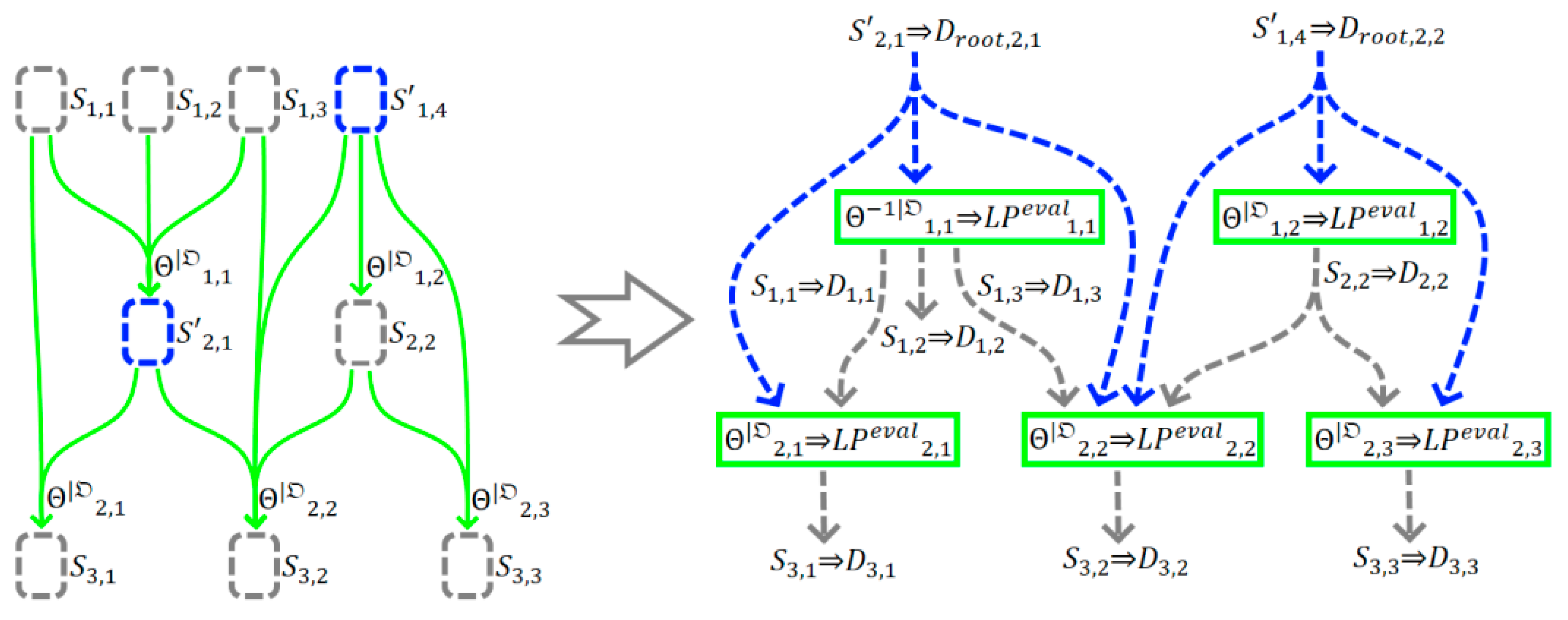
Figure 7.
Addition of and into the computational graph
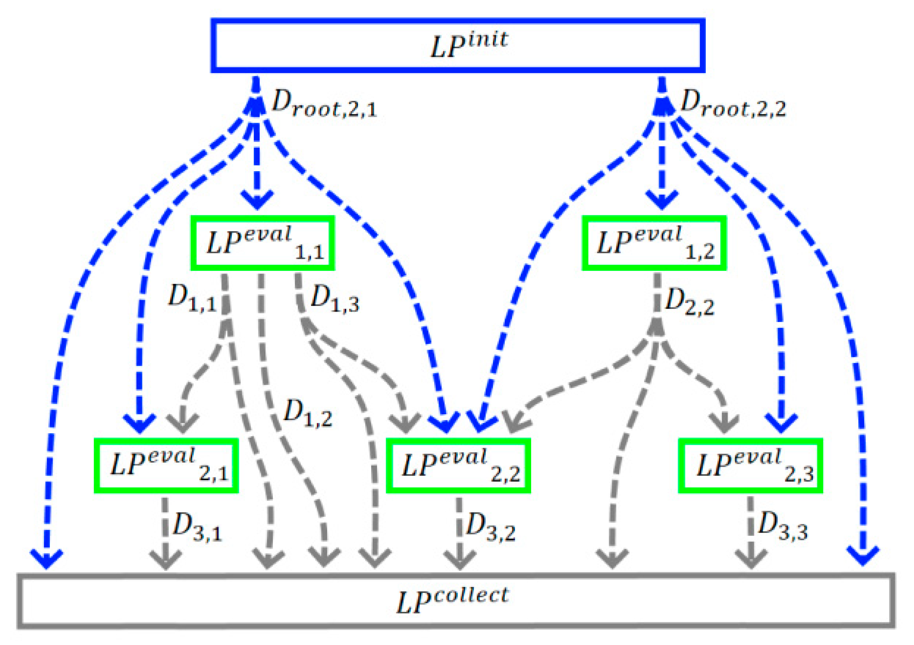
Figure 8.
Example of the folding of the simple computational graph
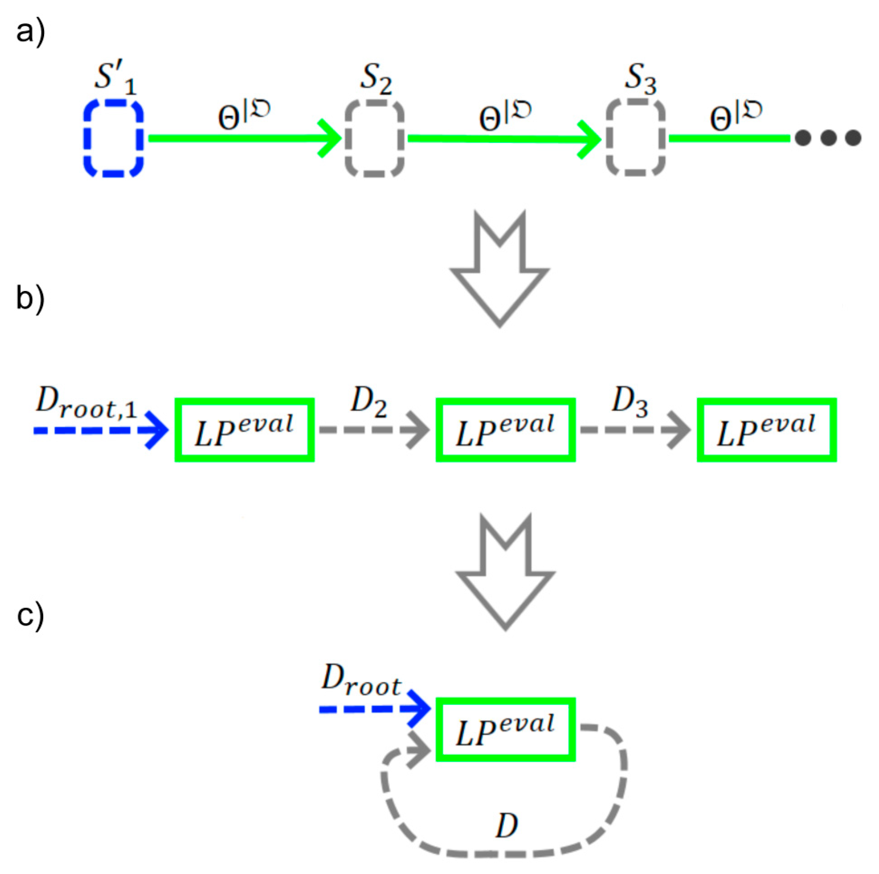
Figure 9.
Example of the folding of a more complex computational graph
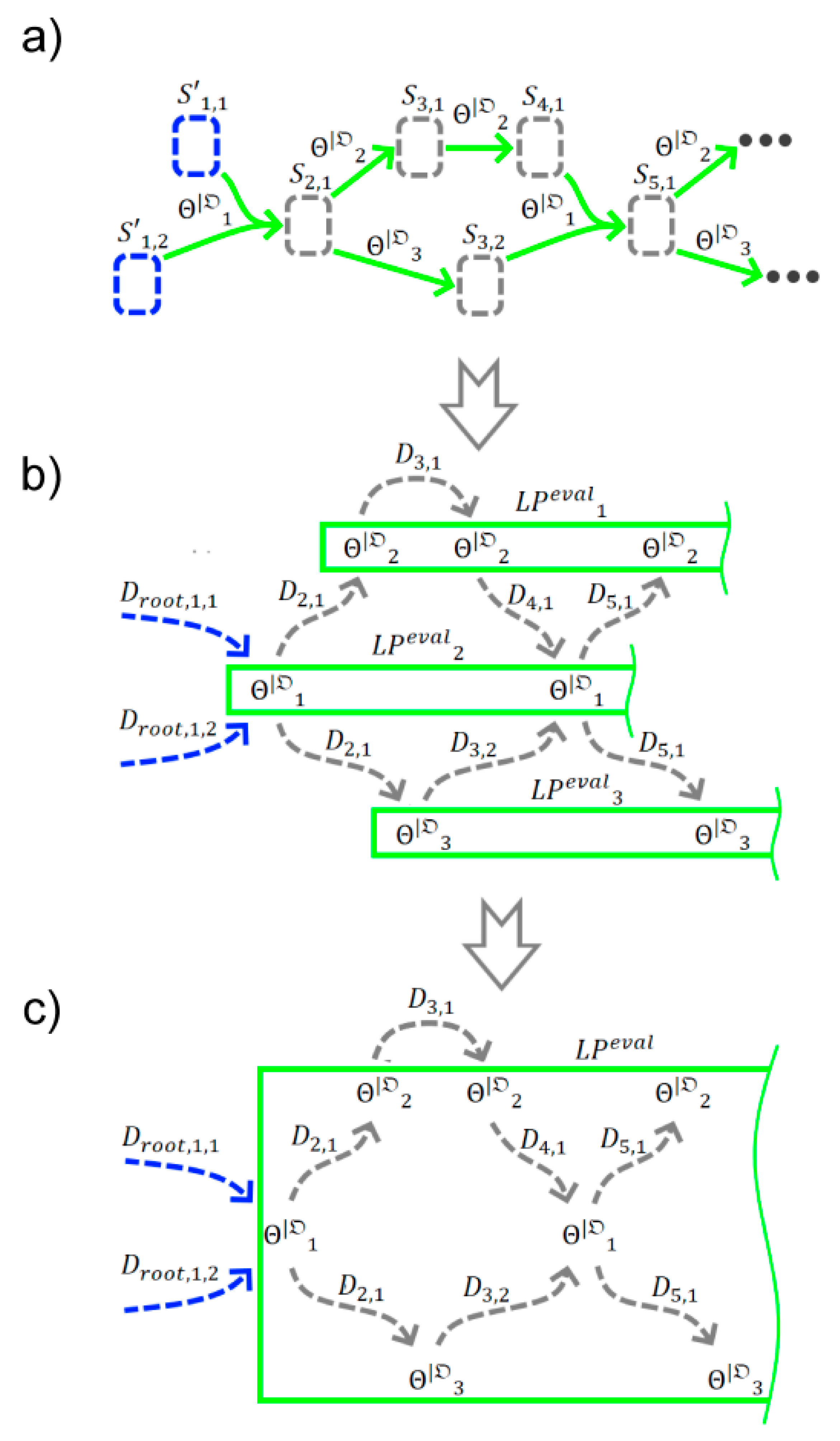
Figure 10.
Results of a simulation of the (first plot) and (second plot) models. Where X axis is time and Y axis is salt concentration, green line is salt concentration in tank 1 and red line is salt concentration in tank 2.
Figure 10.
Results of a simulation of the (first plot) and (second plot) models. Where X axis is time and Y axis is salt concentration, green line is salt concentration in tank 1 and red line is salt concentration in tank 2.
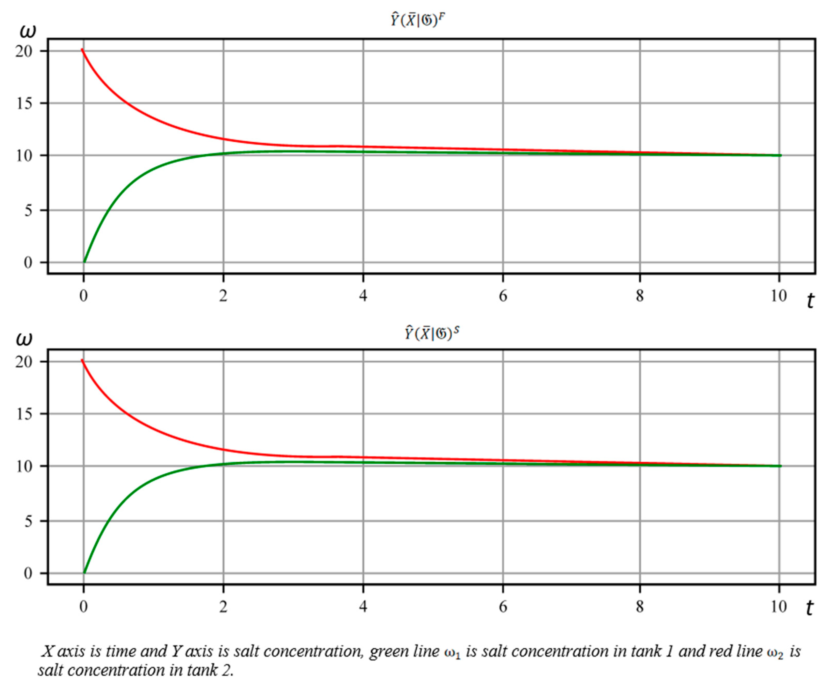
Figure 11.
Simulation of the model using graph . Where X axis is time and Y axis is salt concentration, green line is salt concentration in tank 1 and red line is salt concentration in tank 2, gray line is saline solution concentration supplied to tank 1 constantly.
Figure 11.
Simulation of the model using graph . Where X axis is time and Y axis is salt concentration, green line is salt concentration in tank 1 and red line is salt concentration in tank 2, gray line is saline solution concentration supplied to tank 1 constantly.
Disclaimer/Publisher’s Note: The statements, opinions and data contained in all publications are solely those of the individual author(s) and contributor(s) and not of MDPI and/or the editor(s). MDPI and/or the editor(s) disclaim responsibility for any injury to people or property resulting from any ideas, methods, instructions or products referred to in the content. |
© 2025 by the authors. Licensee MDPI, Basel, Switzerland. This article is an open access article distributed under the terms and conditions of the Creative Commons Attribution (CC BY) license (http://creativecommons.org/licenses/by/4.0/).
Copyright: This open access article is published under a Creative Commons CC BY 4.0 license, which permit the free download, distribution, and reuse, provided that the author and preprint are cited in any reuse.


