
Submitted:
18 April 2025
Posted:
18 April 2025
You are already at the latest version
Abstract
The paper investigates the ability of asset pricing models to explain the cross
section of average stock returns of anomaly portfolios. A large sample of 286 anomaly
portfolios are employed. We perform out-of-sample cross-sectional regression tests of
both prominent asset pricing models and a relatively new model dubbed the ZCAPM.
Empirical tests strongly support the lesser known ZCAPM but not other multifactor
models. Further analyses of out-of-sample mispricing errors of the models reveal
that the ZCAPM provides much more accurate pricing of anomaly portfolios than
other models. We conclude that anomalies are anomalous to popular multifactor
models but not the ZCAPM. By implication, the efficient market hypothesis is supported.
Keywords:
anomalies
; asset pricing models
; mispricing error
; ZCAPM
1. Introduction
In his Presidential Address to the American Finance Association, John Cochrane (2011) observed that a "factor zoo" exists in the field of asset pricing due to the proliferation of stock market anomalies. In a series of papers, Fama and French (1992, 1993, 1996a, 1996b) showed that the now famous capital asset pricing model (CAPM) of Sharpe (1964), Lintner (1965), Mossin (1966), and Treynor (1961, 1962) failed to explain stock returns in general and size and value anomalies in particular. High (low) beta stocks did not have higher (lower) returns than other stocks. In its place, they proposed a three-factor model that augmented the market factor with size and value factors. This innovative multifactor model did a good job of explaining the size and value anomalies.
Subsequently, consistent with Cochrane, researchers discovered hundreds of anomalies, which has evolved into two branches of literature. One branch documents the anomalies and tests for their persistence over time. Work by McLean and Pontiff (2016) investigated 97 anomaly portfolios and found that anomalies tended to diminish or disappear over time after their publication in academic journals. This diminution of anomalies has been confirmed by other researchers.1 By contrast, Jacobs and Müller (2020) examined 241 anomalies in 39 stock markets that (with the exception of the United States) did not tend to diminish in post-publication years. Another study by Chen and Zimmerman (2020) found that prior publication only explains 12 percent of anomaly returns. Also, Jensen, Kelly, and Pedersen (2023) found that 153 long/short factors across 93 countries can be replicated over time, hold on an out-of-sample basis after their original publication, are supported by the large number of factors including global evidence, and can be combined into a smaller number of anomaly clusters. Unlike previous studies, the authors used alphas from the CAPM to measure anomaly returns. They found that risk-adjusted returns yield different results than raw returns. Another recent paper by Bowles, Reed, Ringgenberg, and Thornock (2023) explored the timing of anomalies and found that anomaly returns persist but decay rapidly after information release dates. Previous studies that rebalance anomaly portfolios on an annual basis (for example) incorporate stale information. In their study, using real-time data after information events, anomaly returns did not decrease over time. Hence, they concluded that event-based anomalies were alive and well in financial markets. Consistent with these studies, numerous authors ascribe to the notion that anomalies are real mispricing as opposed to data mining.2
A second branch of studies has sought to address the factor zoo problem by developing parsimonious asset pricing models that can explain many anomalies. For example, to explain 80 anomaly portfolios, Xue, and Zhang (2015) proposed a four-factor model with market, size, profit, and capital investment factors.3 Also, using the same 80 anomaly portfolios, Stambaugh and Yuan (2017) specified a four-factor model with market, size, management, and performance factors that outperformed the Hou, Xue, and Zhang (2015) model in terms of explanatory power. Thus, these studies suggest that low dimension asset pricing models can be used to capture many anomalies.
We extend asset pricing studies by comparing the ability of multifactor models to explain large numbers of anomaly portfolio returns. Surprisingly, standard Fama and MacBeth (1973) cross-sectional regression tests show that a lesser known two-factor model dubbed the ZCAPM by Kolari, Liu, and Huang (2021) well outperforms prominent multifactor models in terms of explaining anomaly returns on an out-of-sample basis. In empirical tests, we utilize online databases of anomalies recently made available by researchers. Chen and Zimmerman (2022) have provided an open source database with 161 long/short anomalies in the U.S. stock market.4 Also, Jensen, Kelly, and Pedersen (2023) have furnished an online database containing153 long/short anomalies in 93 countries including the U.S. Based on 133 anomalies in the former study and 153 anomalies in the latter study with return series available from July 3, 1972 to December 31, 2021, we investigate a combined dataset off 286 anomalies.
We find that, with the exception of the ZCAPM, prominent multifactor models do not explain anomaly portfolio returns. By contrast, the ZCAPM does a much better job of explaining them. In standard Fama and MacBeth (1973) cross-sectional regression tests, factor loadings for the ZCAPM are more significant than well-known multifactor models. Also, goodness-of-fit as estimated by values are much higher for the ZCAPM than other models. Further graphical tests compare the mispricing errors of different models with respect to anomaly portfolios. We find that the ZCAPM exhibits much lower mispricing errors than other models. We conclude that anomaly returns are anomalous for the most part with respect to prominent multifactor models but not the ZCAPM. By implication, our evidence supports the efficient markets hypothesis of Fama (1970, 2013) rather than the behavioral hypothesis.5 As such, stock returns are closely related to systematic market risks.
The next section reviews the methodology. Section 3 reports and discusses the empirical evidence. The last section concludes.
2. Literature Review
The asset pricing literature has evolved over time to produce a wide variety of models to help explain stock market anomalies. Fama and French (1992, 1993) proposed the now famous three-factor model that augmented the market factor with size and value factors. The latter factors were shown to better explain portfolios of stocks sorted on size and value firm characteristics than the CAPM market factor alone. Carhart (1997) added a momentum factor to explain the momentum anomaly. Extending these multifactor models, Fama and French (2015) added profitability and capital investment factors. They found that the value factor could be dropped with similar ability of the resultant four-factor model to explain various anomaly portfolio sorted on size, value, profitability, and capital investment firm characteristics.
Expanding the study of anomalies, Hou, Xue, and Zhang (2015) developed a four-factor model (with factors similar to those in the Fama and French four-factor model. The found that their model outperformed other models in terms of explaining the returns of 80 long/short anomaly portfolios. Like Fama and French, they utilized in-sample Gibbons, Ross, and Shanken (GRS) (1989) test for the joint equality of anomaly portfolios’ alpha estimates. Unlike the present study, they did not report out-of-sample cross-sectional regression test results. Another related study by Stambaugh and Yuan (2017) proposed a four-factor model including market, size, management, and performance factors. Using the same 80 anomaly portfolio as Hou et al., their model outperformed other models in GRS tests of model alphas.
Departing from long/short factors constructed by researechers, Lettau and Pelger (2020) tested a five-factor model based on latent (hidden) factors identified by principal components analysis (PCA). GRS tests showed that their model had lower mispricing errors (as measured by alphas for 370 portfolios sorted on various firm characteristics) than the Fama and French three- and five-factor models. In efforts to improve their model, Fama and French (2018) incorporated a momentum factor to form a six-factor model. This model appeared to perform well in alpha tests relative to their prior multifactor models.
Lastly, Kolari, Liu, and Huang (2021) proposed in a book a new asset pricing model dubbed the ZCAPM derived mathematically as a special case of Black’s (1972) zero-beta CAPM. As reviewed in the next section, the ZCAPM has two factors: (1) beta risk related to average market returns, and (2) zeta risk associated with cross-section market return dispersion. Empirical tests using size and value portfolios employed by Fama and French showed that the ZCAPM consistently outperformed their three-factor model in out-of-sample cross-sectional regression tests, at times by large margins. Additionally, lower average mispricing errors were documented for the ZCAPM than other multifactor models. Further tests of industry portfolio and individual stocks, as well as other anomaly portfolios sorted on firm characteristics, supported the ZCAPM, which outperformed other popular models.
Kolari, Huang, Liu, and Liao (2022) tested the ZCAPM using U.S. stocks for a long sample period from 1927 to 2020. The results confirmed the findings of Kolari et al. (2021). Again in out-of-sample cross-sectional regression tests, the ZCAPM well outperformed the CAPM, Fama and French three-factor model, and Carhart four-factor model. Subperiod results by splitting sample observations continued to support the ZCAPM over the other models. As before, t-statistics corresponding to the market price of zeta risk related to market return dispersion loadings exceeded 3 that were higher than other factors loadings market prices of risk. The authors concluded that the ZCAPM offers a parsimonious empirical model with only two factors and theoretical foundations in the general equilibrium CAPM and zero-beta CAPM asset pricing models.
Kolari, Butt, Huang, Butt, and Liao (2022) conducted tests of the ZCAPM on anomaly portfolios in Canada, France, Germany, Japan, the United Kingdom, and the United States. They compared the ZCAPM to the Fama and French three-factor model and Carhart four-factor model. In all countries, the ZCAPM outperformed these models in out-of-sample cross-sectional regression tests with higher values and t-statistics for zeta risk loadings. Also, average mispricing errors were substantially lower for the ZCAPM relative to the other models. They concluded that the ZCAPM is not a false discovery, which renews interest in the CAPM as a viable approach to asset pricing.
Recently, another book by Kolari, Liu, and Pynnonen (2024) applied the ZCAPM to constructing high return stock portfolios. The CRSP index exhibited much lower Sharpe ratios than these portfolios. Based on their evidence for U.S. stocks, the authors showed that the mean-variance investment parabola of Markowitz (1959) has an architecture that can be mapped in terms of the beta risk and zeta risk of portfolios. The CRSP index and S&P 500 index lied in the middle of their empirical depiction of the mean-variance investment parabola. All portfolios’ returns were computed out-of-sample in the month ahead of the estimation of risk parameters in the ZCAPM. Application of the ZCAPM to actively-managed equity mutual funds showed that the ZCAPM could be used to help guide mutual fund investments by pension funds and other investors. We interpret their finding to suggest that more efficient portfolios with higher Sharpe ratios can be constructed using the ZCAPM to estimate beta risk and zeta risk measures.
3. Methodology
We download daily anomaly portfolio returns from the internet websites of Chen and Zimmerman (2022) and Jensen, Kelly, and Pedersen (2023). Of 161 clear predictor portfolios in the former dataset, 133 anomaly portfolios are retained with available returns from July 3, 1972 to December 31, 2021 6 The latter dataset includes 153 anomaly portfolios with available returns. Appendix A and Appendix B contain lists of anomalies in these two respective databases. Factors for the models under study (to be discussed shortly) are downloaded from Kenneth French’s online database.7
3.1. Cross-Sectional Regression Tests
As already mentioned, we employ standard Fama and MacBeth (1973) tests. First, each model is estimated using a time-series regression. Second, risk loadings of factors in each model are used as independent variables in an out-of-sample (one-month-ahead) cross-sectional regression, which provides estimates of the market price of risk for loadings. More specifically, we begin by estimating the following time-series regression for the ith anomaly portfolio in the one-year estimation window from July 1972 to June 1973:
where is the realized excess return on the ith test asset for day t; is the riskless rate proxied by the Treasury bill rate; is the intercept term or alpha; are asset pricing factors for factors; are corresponding K beta risk loadings for the ith portfolio; correspond to the number of portfolios; is the estimation period; and iid (0, ).
Next, we estimate following out-of-sample cross-sectional regression in the next month of July 1973:
where is the realized excess return on the ith portfolio in out-of-sample (one-month-ahead) month ; is the intercept; are K beta risk loadings estimated for N anomaly portfolios in the estimation period ; are corresponding estimated market prices of beta risk loadings8; and are zero mean and independent of the explanatory variables.
The above two-step process is rolled forward one month at a time and repeated to generate a monthly time-series of market prices of risk, or from July 1973 to December 2021. Subsequently, average market prices of risks and associated t-statistics are computed. Additionally, a monthly time series of realized and predicted returns for each portfolio from July 1973 to December 2021 is produced. Using these series, we compute average realized and average predicted returns for each of the 286 anomaly portfolios. Following Jagannathan and Wang (1996) and Lettau and Ludwigson (2001, footnote 17, p. 1254), a simple cross-sectional regression of average realized returns on average predicted returns is run to yield an estimate of the value. Lastly, we plot average realized returns against predicted returns to graphically illustrate mispricing errors for anomaly portfolios.
3.2. Asset Pricing Models
3.2.1. Prominent Asset Pricing Models
The following leading or renowned asset pricing models are studied:
- CAPM based on the market factor computed using the University of Chicago’s Center for Research in Security Prices (CRSP) value-weighted index minus the Treasury bill rate (M);
- Fama and French (1992, 1993) three-factor model (FF3) that augments the market factor with a size factor (small minus large firms’ stock returns, or SMB) and a value factor (high book-to-market equity minus low book-to-market equity firms’ stock returns, or HML);
- Carhart (1997) four-factor model (C4) that augments the three-factor model with a momentum factor (firms with high past return stock returns minus low past stock returns, or MOM);
- Fama and French (2015) five-factor model (FF5) that augments the three-factor model with a profit factor (robust operating profitability minus weak operating profitability returns, RMW) and capital investment factor (conservative investment minus aggressive investment returns, or CMA);
- Fama and French (2018) six-factor model (FF6) that augments the five-factor model with a momentum factor;
Additionally, we include the little-known Kolari, Liu, and Huang (2021) ZCAPM that augments the market factor with a cross-sectional market return dispersion factor. We next provide an overview of the ZCAPM.
3.2.2. Overview of ZCAPM
Kolari, Liu, and Huang (2021) (hereafter KLH) recently published a book that proposed a new asset pricing model dubbed the ZCAPM.9 Their model is mathematically derived as a special case of Black’s (1972) now famous zero-beta CAPM. Two systematic risk factors emerge from their derivation: (1) average market return in excess of the riskless rate (i.e., market factor); and (2) cross-sectional standard deviation of returns in the market (i.e., market return dispersion). These factors are computed as the first and second moments of stock market returns on any given day. Note that the market dispersion factor is a cross-sectional rather than time-series standard deviation of returns.10 Market return dispersion is computed using the value-weighted CRSP index return (denoted ) on each day t as:
where n is the total number of stocks; is the previous day’s market value weight for the ith stock (i.e., market capitalization of the stock divided by the market capitalization of all n stocks); is the return of the ith stock on day t; and is value-weighted average return of all available stocks in the CRSP database on day t. Many authors associate market return dispersion with macroeconomic shocks, such as economic uncertainty, business cycles, market volatility, and unemployment rates.11
The theoretical ZCAPM is closely related to the now famous mean-variance investment parabola of Markowitz (1952, 1959). KLH. proved that the width or span of the parabola is determined by market return dispersion. Figure 1 shows the parabola with total risk (as measured by the time-series standard deviation of returns) on the X-axis and expected returns on the Y-axis. Interestingly, assuming the width is defined by market return dispersion, it must be true that the average market return lies somewhere along the axis of symmetry that divides the parabola into two symmetric halves. Thus, KLH inferred that the value-weighted CRSP index lies in the middle of the parabola, which is far from the efficient frontier. Many researchers have conjectured that the CRSP index represents an efficient portfolio and, therefore, is a plausible proxy for the market portfolio in Sharpe’s (1964) CAPM. According to the ZCAPM, to reach the efficient frontier, investors should use the average market return to move along the axis of symmetry and then positive market return dispersion to move upward to the efficient frontier. Conversely, to reach the lower inefficient boundary of the parabola, investors can move downward from the axis of symmetry via negative market return dispersion. Importantly, market return dispersion can be positive or negative in sign for assets within the opportunity set described by the parabola.
In Figure 1, KLH chose two portfolios with the same time-series return variance (denoted ) to derive the ZCAPM – namely, efficient portfolio and orthogonal inefficient zero-beta portfolio . Simplifying their derivation, the expected returns of these two portfolios can be specified as follows:12
where is the average market return; and is the market return dispersion.
Sharpe’s CAPM assumed perfect capital markets, homogeneous investor expectations, two-parameter probability distributions of returns, investor risk aversion, no short selling, and a riskless rate. Black amended the last two assumptions to allow short selling and borrowing at a rate greater than the riskless rate. His now famous zero-beta CAPM can be written as:
where is the expected market portfolio return; is the expected zero-beta portfolio return that is uncorrelated (orthogonal) to the market portfolio; and is beta risk associated with excess expected market returns. According to Roll (1972), Copeland and Weston (1980), and others, Black’s model can be more generally specified in terms of any efficient portfolio and its orthogonal inefficient portfolio:
where I and are any efficient index and its orthogonal zero-beta counterpart, respectively, located on the minimum variance boundary of the parabola.
Substituting the expected returns defined in equations (4) and (5) into zero-beta CAPM relation (7), the theoretical ZCAPM is:
where (i.e., the systematic risk of asset i associated with ). Notice that the theoretical ZCAPM is an alternative equivalent form of the zero-beta CAPM with respect to portfolios and . Lastly, assuming the existence of a riskless rate asset, the theoretical ZCAPM can be respecified as:13
where captures beta risk related to expected market excess returns; and is zeta risk associated with cross-sectional market return dispersion of expected returns of all assets in the market. As noted above, zeta risk can be positive or negative in sign with respect to the expected returns of portfolios and , respectively.
In the ZCAPM, as the the width of the parabola increases or decreases due to , the expected returns of assets within the parabola are affected. As increases (decreases), assets in the upper half of the parabola above the axis of symmetry experience increasing (decreasing) expected returns; alternatively, assets in the bottom half of the parabola below the axis of symmetry experience decreasing (increasing) expected returns. It is obvious that market return dispersion has major impacts of the expected returns of assets in the market. Also, depending where assets are located within the parabola, these dispersion impacts can be positive or negative.
A major challenge for the ZCAPM is the specification of an empirical model that can capture both positive and negative market dispersion effects on assets’ returns. KLH proposed an innovative solution to this problem by introducing a hidden signal variable to model these two-sided dispersion effects:
where measures systematic risk associated with market return dispersion ; is a hidden signal variable.14 is assigned values and to coincide with positive and negative market return dispersion effects on asset returns at time t, respectively; is the intercept related to mispricing errors; ; and other notation is as before. In forthcoming analyses, we proxy average market returns, or , with the value-weighted CRSP index return. Also, we proxy the market return dispersion using all common stocks in the CRSP database per Equation (3).
Unlike virtually all asset pricing models that employ ordinary least squares (OLS) regression, the empirical ZCAPM is estimated by means of the expectation-maximization (EM) algorithm, which is well known in the hard sciences.15 EM provides an estimate of the probability that hidden signal variable is (p) or (.16 In empirical ZCAPM regression relation (11), is an independent random variable with a two-point distribution:
where (or ) is the probability of a positive (or negative) market return dispersion effect; and are independent of . The EM algorithm estimates probability using available in-sample information about the dependent and independent variables in the model.
Based on equation (10), can take on values of or due to the sign of . Since the mean of binary signal variable equals , we can define . The parameter captures the systematic risk related to market return dispersion . Hence, the empirical ZCAPM can be written as:
where and proxy beta risk and zeta risk parameters in the theoretical ZCAPM. In sample period , the sign of is based on the estimated probability of hidden variable . Hence, if , the sign of is positive (negative). The empirical ZCAPM as estimated via EM is a probabilistic mixture model with two components, wherein one component has positive zeta risk and the other component has negative zeta risk.
We should mention that some authors have augmented the market factor with a market return dispersion factor, including Jiang (2010), Demirer and Jategaonkar (2013), and Garcia, Mantilla-Garcia, and Martellini (2014). Using OLS regression to estimate the time-series regression model and subsequent cross-sectional regression tests of factor loadings, they found both positive and negative sensitivity of stock returns to market return dispersion factor loadings. Sometimes the latter factor loadings associated with market return dispersion were significant but not in other tests. We have found in repeated tests of the ZCAPM using many different test assets and sample time periods that zeta risk loadings are always significant in cross-sectional regression tests at high statistical levels that well exceed previous studies.
Unlike OLS regression asset pricing models, KLH found that the intercept parameter (or alpha) can be dropped from the empirical ZCAPM. No decrease in residual error variance was achieved by adding an intercept. For interested readers, KLH provide open source empirical ZCAPM software using Matlab, R, and Python programs on the internet at GitHub (https://Github.com/zcapm). Programs for running Fama-MacBeth cross-sectional regression tests are available at this website also.
Finally, ZCAPM factor loadings for and based on one year of daily returns prior to month are used to estimate the following OLS cross-sectional regression:
where is the intercept term, and are estimates of the market prices of beta risk and zeta risk loadings in percent terms, respectively, and other notation is as before. It is notable that the dependent variable in this regression is the one-month ahead excess returns for the ith anomaly portfolio. Since zeta risk loadings are estimated using daily returns, we rescale the estimated zeta risk coefficient from a daily to monthly basis as follows:
where is the number of trading days in month (i.e., 21 days), is the monthly estimated zeta risk, and is the monthly risk premium associated with zeta risk. This rescaling does not change the risk premium in terms of each unit of zeta risk. Now the estimated monthly market price of , or , can be compared to the estimated monthly market price of , or .
4. Empirical Evidence
In this section, we report the results of cross-sectional regression tests of asset pricing models as well as comparative graphs of their average mispricing errors. Table 1 reports descriptive statistics for asset pricing factors in different models in our sample period. The market return dispersion factor computed using Equation (3) is denoted as RD.
4.1. Cross-Sectional Regression Results
Table 2 documents that empirical results from OLS cross-sectional regression tests for different asset pricing models. As shown there, the CAPM has almost no explanatory power with only a 1 percent value. The market price of market beta loadings, or , is zero and far from statistical significance. Comparatively, the Fama and French three-factor model noticeably improves matters. The value increases to 11 percent and the market price of value beta risk loadings, or , is significant at the 10 percent level. The results are little changed for the Carhart four-factor model. The Fama and French five- and six-factor models exhibit some improvement in both explanatory power and statistical significance. The six-factor model boosts to 19 percent. Also, capital investment factor loadings, or , are significant at the 1 percent level or lower.
Turning to the ZCAPM, the results are much stronger than the other models. Now the value jumps to 84 percent. This very high goodness-of-fit suggests that the ZCAPM well explains anomaly portfolio returns. Given the fact that our tests are out-of-sample in the month ahead of the period used to estimate beta risk and zeta risk loadings, this explanatory power is exceptional.
For the ZCAPM, the market price of zeta risk loadings associated with market return dispersion, or , is very significant with a t-statistic of 6.69. To the authors’ knowledge, no prior asset pricing studies have reported a t-statistic of this magnitude with respect to systematic risk loadings. In this regard, Harvey, Liu, and Zhu (2016) and Chordia, Goyal, and Saretto (2020) have recommended a t-statistic threshold of 3 to avoid false discoveries of significant asset pricing factors. Since exceeds 6, we infer that market return dispersion is an extremely significant asset pricing factor. Furthermore, the estimated magnitudes of and associated with beta risk and zeta risk loadings, respectively, are economically significant at 0.30 percent and 0.72 percent per month, or 3.60 percent and 8.64 percent per year.
As a robustness check, we re-ran the analyses using a full sample period regression approach, rather than a one-month rolling regression approach. Using the full period from July 1972 to December 2021, we estimate the empirical ZCAPM. Subsequently, we estimate cross-sectional regressions in each month and average the monthly results. In unreported results, our findings are unchanged for the most part. The market prices of beta and zeta risk loadings, or and , respectively, are 0.45 percent and 1.32 percent with significant t-statistics equal to 2.21 and 8.62. The value is estimated at 86 percent. Other models’ results improve somewhat also but are again much weaker than those for the ZCAPM. Interestingly, when we ran daily cross-sectional regressions in the full sample period and average the results, the t-statistic associated with the market price of zeta risk loadings surges to 13.69, which is even more significant than before. It is clear that zeta risk is important to explaining the cross section of average anomaly portfolio returns.
In sum, stock market anomaly portfolios’ returns are well explained by beta risk and zeta risk in the empirical ZCAPM. Contrarily, the CAPM has no explanatory ability, and prominent multifactor models have far less explanatory ability than the ZCAPM. It is noteworthy that our out-sample cross-sectional regression results cannot be compared to prior multifactor model studies reviewed in Section 2 as they primarily only reported in-sample GRS tests to evaluate different asset pricing models. We believe that out-of-sample tests allow enable a better understanding of the pricing ability of models that is more consonant with real world investor experience. That is, investors measure the risk of assets that they purchase and then observe their performance after portfolio formation. Thus, unlike in-sample tests, out-of-sample tests are akin to an investable market strategy.
4.2. Graphical Mispricing Error Results
According to Fama and MacBeth (1973), a normative model that helps investors make better return/risk decisions is valid to the extent that it can utilize past information to explain future returns. In line with this logic, Cochrane (1996) and Lettau and Ludvigson (2001) have highlighted the comparative analyses of predicted versus realized (actual) returns to evaluate mispricing errors in asset pricing models. As Cochrane has asserted, "Expected return pricing errors ... are a useful characterization of a model’s performance."(Cochrane, 1996, p. 596) In conducting these analyses, he recommended that " ... it is important to examine a model’s ability to explain the expected returns of economically interesting portfolios." (Cochrane, 1996, p. 598) Of course, because anomaly portfolios are difficult for asset pricing models to explain, they are compelling test assets to investigate.
As described earlier, we compute mispricing errors on an out-of-sample basis based on one-month-ahead cross-sectional regressions. Using one year of daily returns for the 286 anomaly portfolios, a time-series regression is run to estimate each asset pricing model and its factor loadings. In the second step, we estimate an out-of-sample (one-month-ahead) cross-sectional regression using one-month-ahead excess returns for anomaly portfolios. By rolling forward one month at a time, this process generates cross-sectional regressions from July 1973 to December 2021. In the next month for each portfolio, we utilize the average of the estimated factor prices of risk and average estimated loadings for the ith portfolio to compute average fitted excess returns. Lastly, for each asset pricing model, a graph is created with average fitted excess returns plotted against each portfolio’s one-month-ahead average actual excess returns.
Figure 2, Figure 3 and Figure 4 illustrate the average pricing errors of different asset pricing models. In Figure 2, we see that both the CAPM and Fama and French three-factor model exhibit large mispricing errors. Instead of pricing errors lining up on the 45 degree line, they are densely populated around the line in a vertical pattern.
As shown in Figure 3, the Carhart four-factor model and Fama and French five-factor model do not improve matters much. By casual observation, the pricing errors for the 286 anomaly portfolios are large in both models.
Finally, Figure 4 compares the Fama and French six-factor model to the ZCAPM. While the six-factor model improves upon the five-factor model in terms of lower mispricing errors, the ZCAPM makes a quantum leap in pricing. Indeed, no anomaly portfolio lies far off the 45 degree line. This level of out-of-sample pricing is exceptional. One would expect that some anomalies would be difficult to price and, therefore, would be located well off the line. In this case, winsorizing the data for eliminate spurious outliers would be useful to investigate. However, because virtually all of the anomaly portfolios are well explained by the ZCAPM, we did not winsorize the data. It is noteworthy that these mispricing error results are based on out-of-sample tests that employ beta risk and zeta risk estimated in a prior one year period to compute fitted or predicted returns in the next month. In effect, future returns are lining up almost exactly with previously estimated systematic risks via the ZCAPM!
The major implication of these graphical analyses is that the 286 anomaly portfolios are anomalous to other asset pricing models but not the ZCAPM. In effect, there none of these portfolios is anomalous from the perspective of the ZCAPM. We infer that researchers will have to expand their search for long/short anomalies in the stock market.
4.3. What Explains ZCAPM Outperformance?
The clear outperformance of the ZCAPM relative to prominent asset pricing models published in top tier finance journals is impressive. What explains this outperformance? According to KLH, long/short factors in multifactor models are rough measures of cross-sectional market return dispersion. For example, the size factor is long higher yielding small stocks and short lower yielding large stocks. It is likely that small stocks are located in the upper half of the mean-variance investment parabola, whereas large stocks are somewhere in the lower half of the parabola. As the parabola widens (narrows), the size factor experiences higher (lower) returns. This two-sided volatility effect is tantamount to the market return dispersion factor in the ZCAPM. However, the long/short size factor is only a slice or piece of the total market return dispersion (or ) in the ZCAPM.
Other multifactors account for other slices within the total market return dispersion that defines the width or span of the mean-variance parabola. As long/short factors are added to multifactor models, they will gradually converge to the total market return dispersion of the ZCAPM. However, long/short factors tend to be unstable over time. If large stocks and small stocks switch their positions in the parabola, then the size factor would flip from being positively priced to being negatively priced. Some studies have observed this pricing behavior for the size factor. Also, a factor could be significant in one time period but not in other periods as the locations of long and short portfolios in the factor move around in the parabola over time.17
KLH have argued that all multifactors are contained within total market return dispersion. There is no need to use all these factors and look for new factors – the factor zoo is captured by market return dispersion. In turn, the ZCAPM measures their aggregate systematic risk in zeta risk.
An important implication of these insights is that multifactor models are related to the ZCAPM. All multifactor models, including the ZCAPM, employ cross-sectional return dispersion in stock returns to explain asset prices. Moreover, in view of this association, we can link multifactor models to the CAPM, as the ZCAPM is mathematically derived from the zero-beta CAPM. According to KLH, the ZCAPM provides a unifying theory and empirical methodology in the field of asset pricing.
It is interesting that Black (1995) later discussed the second beta factor in his zero-beta CAPM. In this words, the second beta factor is " ... the minimum-variance, zero-beta portfolio of risky assets, where beta is defined using whatever market portfolio we use to represent the first factor." (Black, 1995, p. 170). He reasoned as follows:
"When Fama and French say that the line relating expected return and beta is flat,they are just saying that the expected excess return on the second factor is large.If we believe it’s as large as they say, we won’t fool around with their third and fourthfactors, for which they give no theory.18 We’ll go for the gold in the second factor!"
KLH conjectured that market return dispersion corresponds to Black’s second factor. Figure 1 illustrates his second factor as the difference between the returns of an efficient portfolio and inefficient, zero-beta portfolio (with equal return variance), or market return dispersion. It is not necessary to know the expected returns in these two portfolios as their difference corresponds to total market return dispersion. An important policy implication of the ZCAPM relevant to investors is that zeta risk related to market return dispersion is a salient second risk measure (in addition to beta risk associated with the market factor when evaluating the return performance of stock portfolios.
Finally, the relatively accurate pricing of large numbers of anomaly portfolios by the ZCAPM strongly supports the efficient market hypothesis. As observed by Schwert (2003), Fama and French (2008), Fama (2013) and others, stock market anomalies could be explained by a bad model problem in asset pricing or an inefficient market. The existence of a valid model would confirm that the market is efficient. Echoing this observation, the authors of a recent asset pricing study noted that " ... the credibility of the anomalies literature can improve via a close connection with economic theory." (Hou, Xue, and Zhang (2020, p. 2072)) In this regard, our empirical tests and results of the ZCAPM for anomaly portfolios establish a connection to general equilibrium asset pricing theory.
5. Conclusion
This paper sought to compare the ability of different asset pricing models to explain stock market anomaly portfolio returns. We employed a large dataset of 286 anomaly portfolios provided by Chen and Zimmerman (2022) and Jensen, Kelly, and Pedersen (2023). Anomalies are economically interesting due to the fact that they are difficult for asset pricing models to explain.
Surprisingly, virtually all of the anomaly portfolios were well explained the ZCAPM, a recent model proposed by Kolari, Liu, and Huang (2021). In stark contrast, the CAPM as well as a number of prominent multifactor models could not explain anomaly portfolio returns for the most part. Mispricing errors were large for the latter models compared to relatively small pricing errors for the ZCAPM.
We conclude that, given the ZCAPM, long/short stock market anomaly portfolios under study are no longer anomalies. Given the ability of the ZCAPM to explain large datasets of anomalies, our findings support the efficient markets hypothesis. The scope of our study is limited to U.S. stock market anomalies. Further research is recommended on stock market anomalies in other countries as well as other classes of assets, including bonds, commodities, and other asset traded on a daily basis. Also, an important implication for future research is the search to identify long/short stocks portfolios not explained by the ZCAPM. Perhaps behavioral explanations of these anomalies are possible.
Appendix A. 133 Anomaly Portfolios from Chen and Zimmerman (2022)

| N | Abbreviation | Description |
|---|---|---|
| 1 | AbnormalAccruals ret | Abnormal accruals |
| 2 | Accruals ret | Accruals |
| 3 | AdExp ret | Advertisement expense |
| 4 | AM ret | Total assets to market |
| 5 | AnnouncementReturn ret | Earnings announcement return |
| 6 | AssetGrowth ret | Asset growth |
| 7 | Beta ret | CAPM beta |
| 8 | BetaFP ret | Frazzini-Pedersen beta |
| 9 | BetaTailRisk ret | Tail risk beta |
| 10 | BidAskSpread ret | Bid-ask spread |
| 11 | BM ret | Book to market using most recent ME |
| 12 | BMdec ret | Book to market using December ME |
| 13 | BookLeverage ret | Book leverage (annual) |
| 14 | BPEBM ret | Leverage component of BM |
| 15 | BrandInvest ret | Brand capital investment |
| 16 | Cash ret | Cash to assets |
| 17 | CashProd ret | Cash productivity |
| 18 | CBOperProf ret | Cash-based operating profitability |
| 19 | CF ret | Cash flow to market |
| 20 | Cfp ret | Operating cash flows to price |
| 21 | ChAssetTurnover ret | Change in asset turnover |
| 22 | ChEQ ret | Growth in book equity |
| 23 | ChInv ret | Inventory growth |
| 24 | ChInvIA ret | Change in capital investment (industry adjusted) |
| 25 | ChNNCOA ret | Change in net noncurrent operating assets |
| 26 | ChNWC ret | Change in net working capital |
| 27 | ChTax ret | Change in taxes |
| 28 | CompEquIss ret | Composite equity issuance |
| 29 | CompositeDebtIssuance ret | Composite debt issuance |
| 30 | Coskewness ret | Coskewness |
| 31 | DelCOA ret | Change in current operating assets |
| 32 | DelCOL ret | Change in current operating liabilities |
| 33 | DelEqu ret | Change in equity to assets |
| 34 | DelFINL ret | Change in financial liabilities |
| 35 | DelLTI ret | Change in long-term investment |
| 36 | DelNetFin ret | Change in net financial assets |
| 37 | DNoa ret | Change in net operating assets |
| 38 | DolVol ret | Past trading volume |
| 39 | EarningsConsistency ret | Earnings consistency |
| 40 | EarningsSurprise ret | Earnings surprise |
| 41 | EarnSupBig ret | Earnings surprise of big firms |
| 42 | EBM ret | Enterprise component of BM |
| 43 | EntMult ret | Enterprise multiple |
| 44 | EP ret | Earnings-to-Price ratio |
| 45 | EquityDuration ret | Equity duration |
| 46 | FirmAge ret | Firm age based on CRSP |
| 47 | Frontier ret | Efficient frontier index |
| 48 | GP ret | Gross profits/total assets |
| 49 | GrAdExp ret | Growth in advertising expenses |
| 50 | Grcapx ret | Change in capex (two years) |
| 51 | Grcapx3y ret | Change in capex (three years) |
| 52 | GrLTNOA ret | Growth in long term operating assets |
| 53 | GrSaleToGrInv ret | Sales growth over inventory growth |
| 54 | GrSaleToGrOverhead ret | Sales growth over overhead growth |
| 55 | Herf ret | Industry concentration (sales) |
| 56 | HerfAsset ret | Industry concentration (assets) |
| 57 | HerfBE ret | Industry concentration (equity) |
| 58 | High52 ret | 52 week high |
| 59 | Hire ret | Employment growth |
| 60 | IdioRisk ret | Idiosyncratic risk |
| 61 | IdioVol3F ret | Idiosyncratic risk (3 factor) |
| 62 | IdioVolAHT ret | Idiosyncratic risk (AHT) |
| 63 | Illiquidity ret | Amihud’s illiquidity |
| 64 | IndMom ret | Industry momentum |
| 65 | IndRetBig ret | Industry return of big firms |
| 66 | IntanBM ret | Intangible return using BM |
| 67 | IntanCFP ret | Intangible return using CFtoP |
| 68 | IntanEP ret | Intangible return using EP |
| 69 | IntanSP ret | Intangible return using Sale2P |
| 70 | IntMom ret | Intermediate momentum |
| 71 | Investment ret | Investment to revenue |
| 72 | InvestPPEInv ret | Change in PPE and inventory/assets |
| 73 | InvGrowth ret | Inventory growth |
| 74 | Leverage ret | Market leverage |
| 75 | LRreversal ret | Long-run reversal |
| 76 | MaxRet ret | Maximum return over month |
| 77 | MeanRankRevGrowth ret | Revenue growth rank |
| 78 | Mom6m ret | Momentum (6 month) |
| 79 | Mom12m ret | Momentum (12 month) |
| 80 | Mom12mOffSeason ret | Momentum without the seasonal part |
| 81 | MomOffSeason ret | Off season long-term reversal |
| 82 | MomOffSeason06YrPlus ret | Off season reversal years 6 to 10 |
| 83 | MomOffSeason11YrPlus ret | Off season reversal years 11 to 15 |
| 84 | MomOffSeason16YrPlus ret | Off season reversal years 16 to 20 |
| 85 | MomSeason ret | Return seasonality years 2 to 5 |
| 86 | MomSeason06YrPlus ret | Return seasonality years 6 to 10 |
| 87 | MomSeason11YrPlus ret | Return seasonality years 11 to 15 |
| 88 | MomSeason16YrPlus ret | Return seasonality years 16 to 20 |
| 89 | MomSeasonShort ret | Return seasonality last year |
| 90 | MRreversal ret | Medium-run reversal |
| 91 | NetDebtFinance ret | Net debt financing |
| 92 | NetDebtPrice ret | Net debt to price |
| 93 | NetEquityFinance ret | Net equity financing |
| 94 | NetPayoutYield ret | Net payout yield |
| 95 | NOA ret | Net operating asset |
| 96 | NumEarnIncrease ret | Earnings streak length |
| 97 | OperProf ret | Operating profits/book equity |
| 98 | OperProfRD ret | Operating profitability R&D adjusted |
| 99 | OPLeverage ret | Operating leverage |
| 100 | OrderBacklog ret | Order backlog |
| 101 | OrderBacklogChg ret | Change in order backlog |
| 102 | OrgCap ret | Organizational capital |
| 103 | PayoutYield ret | Payout yield |
| 104 | PctAcc ret | Percent operating accruals |
| 105 | Price ret | Price |
| 106 | PS ret | Piotroski F-score |
| 107 | RD ret | R&D over market cap |
| 108 | RDAbility ret | R&D ability |
| 109 | Realestate ret | Real estate holdings |
| 110 | ResidualMomentum ret | Momentum based on FF3 model residuals |
| 111 | ReturnSkew ret | Return skewness |
| 112 | ReturnSkew3F ret | Idiosyncratic skewness (3 factor model) |
| 113 | RevenueSurprise ret | Revenue surprise |
| 114 | Roaq ret | Return on assets (qtrly) |
| 115 | RoE ret | Net income/book equity |
| 116 | ShareIss1Y ret | Share issuance (1 year) |
| 117 | ShareIss5Y ret | Share issuance (5 year) |
| 118 | Size ret | Size |
| 119 | SP ret | Sales-to-price |
| 120 | Std turn ret | Share turnover volatility |
| 121 | STreversal ret | Short term reversal |
| 122 | Tang ret | Tangibility |
| 123 | Tax ret | Taxable income to income |
| 124 | TotalAccruals ret | Total accruals |
| 125 | TrendFactor ret | Trend in the general stock market |
| 126 | VarCF ret | Cash-flow to price variance |
| 127 | VolMkt ret | Volume to market equity |
| 128 | VolSD ret | Volume variance |
| 129 | VolumeTrend ret | Volume trend |
| 130 | XFIN ret | Net external financing |
| 131 | Zerotrade ret | Days with zero trades |
| 132 | ZerotradeAlt1 ret | Days with zero trades |
| 133 | ZerotradeAlt12 ret | Days with zero trades |
Appendix B. 153 Anomaly Portfolios from Jensen, Kelly, and Pedersen (2023)
| N | Anomaly abbreviation | Description |
|---|---|---|
| 1 | capex abn | Abnormal corporate investment |
| 2 | z score | Altman Z-score |
| 3 | ami 126d | Amihud measure |
| 4 | at gr1 | Asset growth |
| 5 | tangibility | Asset tangibility |
| 6 | sale bev | Assets turnover |
| 7 | at me | Assets-to-market |
| 8 | at be | Book leverage |
| 9 | bev mev | Book-to-market enterprise value |
| 10 | be me | Book-to-market equity |
| 11 | capx gr1 | CAPEX growth (1 year) |
| 12 | capx gr2 | CAPEX growth (2 years) |
| 13 | capx gr3 | CAPEX growth (3 years) |
| 14 | at turnover | Capital turnover |
| 15 | ocfq saleq std | Cash flow volatility |
| 16 | cop at | Cash-based operating profits-to-book assets |
| 17 | cop atl1 | Cash-based operating profits-to-lagged book assets |
| 18 | cash at | Cash-to-assets |
| 19 | dgp dsale | Change gross margin minus change sales |
| 20 | be gr1a | Change in common equity |
| 21 | coa gr1a | Change in current operating assets |
| 22 | col gr1a | Change in current operating liabilities |
| 23 | cowc gr1a | Change in current operating working capital |
| 24 | fnl gr1a | Change in financial liabilities |
| 25 | lti gr1a | Change in long-term investments |
| 26 | lnoa gr1a | Change in long-term net operating assets |
| 27 | nfna gr1a | Change in net financial assets |
| 28 | nncoa gr1a | Change in net noncurrent operating assets |
| 29 | noa gr1a | Change in net operating assets |
| 30 | ncoa gr1a | Change in noncurrent operating assets |
| 31 | ncol gr1a | Change in noncurrent operating liabilities |
| 32 | ocf at chg1 | Change in operating cash flow to assets |
| 33 | niq at chg1 | Change in quarterly return on assets |
| 34 | niq be chg1 | Change in quarterly return on equity |
| 35 | sti gr1a | Change in short-term investments |
| 36 | ppeinv gr1a | Change PPE and Inventory |
| 37 | dsale dinv | Change sales minus change Inventory |
| 38 | dsale drec | Change sales minus change receivables |
| 39 | dsale dsga | Change sales minus change SG&A |
| 40 | dolvol var 126d | Coefficient of variation for dollar trading volume |
| 41 | turnover var 126d | Coefficient of variation for share turnover |
| 42 | coskew 21d | Coskewness |
| 43 | prc highprc 252d | Current price to high price over last year |
| 44 | debt me | Debt-to-market |
| 45 | beta dimson 21d | Dimson beta |
| 46 | div12m me | Dividend yield |
| 47 | dolvol 126d | Dollar trading volume |
| 48 | betadown 252d | Downside beta |
| 49 | ni ar1 | Earnings persistence |
| 50 | earnings variability | Earnings variability |
| 51 | ni ivol | Earnings volatility |
| 52 | ni me | Earnings-to-price |
| 53 | ebitda mev | Ebitda-to-market enterprise value |
| 54 | eq dur | Equity duration |
| 55 | eqnpo 12m | Equity net payout |
| 56 | age | Firm age |
| 57 | betabab 1260d | Frazzini-Pedersen market beta |
| 58 | fcf me | Free cash flow-to-price |
| 59 | gp at | Gross profits-to-assets |
| 60 | gp atl1 | Gross profits-to-lagged assets |
| 61 | debt gr3 | Growth in book debt (3 years) |
| 62 | rmax5 21d | Highest 5 days of return |
| 63 | rmax5 rvol 21d | Highest 5 days of return scaled by volatility |
| 64 | emp gr1 | Hiring rate |
| 65 | iskew capm 21d | Idiosyncratic skewness from the CAPM |
| 66 | iskew ff3 21d | Idiosyncratic skewness from the Fama-French 3-factor model |
| 67 | iskew hxz4 21d | Idiosyncratic skewness from the q-factor model |
| 68 | ivol capm 21d | Idiosyncratic volatility from the CAPM (21 days) |
| 69 | ivol capm 252d | Idiosyncratic volatility from the CAPM (252 days) |
| 70 | ivol ff3 21d | Idiosyncratic volatility from the Fama-French 3-factor model |
| 71 | ivol hxz4 21d | Idiosyncratic volatility from the q-factor model |
| 72 | ival me | Intrinsic value-to-market |
| 73 | inv gr1a | Inventory change |
| 74 | inv gr1 | Inventory growth |
| 75 | kz index | Kaplan-Zingales index |
| 76 | sale emp gr1 | Labor force efficiency |
| 77 | aliq at | Liquidity of book assets |
| 78 | aliq mat | Liquidity of market assets |
| 79 | ret 60 12 | Long-term reversal |
| 80 | beta 60m | Market beta |
| 81 | corr 1260d | Market correlation |
| 82 | market equity | Market equity |
| 83 | rmax1 21d | Maximum daily return |
| 84 | mispricing mgmt | Mispricing factor: Management |
| 85 | mispricing perf | Mispricing factor: Performance |
| 86 | dbnetis at | Net debt issuance |
| 87 | netdebt me | Net debt-to-price |
| 88 | eqnetis at | Net equity issuance |
| 89 | noa at | Net operating assets |
| 90 | eqnpo me | Net payout yield |
| 91 | chcsho 12m | Net stock issues |
| 92 | netis at | Net total issuance |
| 93 | ni inc8q | Number of consecutive quarters with earnings increases |
| 94 | zero trades 21d | Number of zero trades with turnover as tiebreaker (1 month) |
| 95 | zero trades 252d | Number of zero trades with turnover as tiebreaker (12 months) |
| 96 | zero trades 126d | Number of zero trades with turnover as tiebreaker (6 months) |
| 97 | o score | Ohlson O-score |
| 98 | oaccruals at | Operating accruals |
| 99 | ocf at | Operating cash flow to assets |
| 100 | ocf me | Operating cash flow-to-market |
| 101 | opex at | Operating leverage |
| 102 | op at | Operating profits-to-book assets |
| 103 | ope be | Operating profits-to-book equity |
| 104 | op atl1 | Operating profits-to-lagged book assets |
| 105 | ope bel1 | Operating profits-to-lagged book equity |
| 106 | eqpo me | Payout yield |
| 107 | oaccruals ni | Percent operating accruals |
| 108 | taccruals ni | Percent total accruals |
| 109 | f score | Pitroski F-score |
| 110 | ret 12 1 | Price momentum t-12 to t-1 |
| 111 | ret 12 7 | Price momentum t-12 to t-7 |
| 112 | ret 3 1 | Price momentum t-3 to t-1 |
| 113 | ret 6 1 | Price momentum t-6 to t-1 |
| 114 | ret 9 1 | Price momentum t-9 to t-1 |
| 115 | prc | Price per share |
| 116 | ebit sale | Profit margin |
| 117 | qmj | Quality minus Junk: Composite |
| 118 | qmj growth | Quality minus Junk: Growth |
| 119 | qmj prof | Quality minus Junk: Profitability |
| 120 | qmj safety | Quality minus Junk: Safety |
| 121 | niq at | Change in quarterly return on assets |
| 122 | niq be | Quarterly return on equity |
| 123 | rd5 at | R&D capital-to-book assets |
| 124 | rd me | R&D-to-market |
| 125 | rd sale | R&D-to-sales |
| 126 | resff3 12 1 | Residual momentum t-12 to t-1 |
| 127 | resff3 6 1 | Residual momentum t-6 to t-1 |
| 128 | ni be | Return on equity |
| 129 | ebit bev | Return on net operating assets |
| 130 | rvol 21d | Return volatility |
| 131 | saleq gr1 | Sales growth (1 quarter) |
| 132 | sale gr1 | Sales growth (1 year) |
| 133 | sale gr3 | Sales growth (3 years) |
| 134 | sale me | Sales-to-market |
| 135 | turnover 126d | Share turnover |
| 136 | ret 1 0 | Short-term reversal |
| 137 | niq su | Standardized earnings surprise |
| 138 | saleq su | Standardized Revenue surprise |
| 139 | tax gr1a | Tax expense surprise |
| 140 | pi nix | Taxable income-to-book income |
| 141 | bidaskhl 21d | The high-low bid-ask spread |
| 142 | taccruals at | Total accruals |
| 143 | rskew 21d | Total skewness |
| 144 | seas 1 1an | Year 1-lagged return, annual |
| 145 | seas 1 1na | Year 1-lagged return, nonannual |
| 146 | seas 2 5an | Years 2-5 lagged returns, annual |
| 147 | seas 2 5na | Years 2-5 lagged returns, nonannual |
| 148 | seas 6 10an | Years 6-10 lagged returns, annual |
| 149 | seas 6 10na | Years 6-10 lagged returns, nonannual |
| 150 | seas 11 15an | Years 11-15 lagged returns, annual |
| 151 | seas 11 15na | Years 11-15 lagged returns, nonannual |
| 152 | seas 16 20an | Years 16-20 lagged returns, annual |
| 153 | seas 16 20na | Years 16-20 lagged returns, nonannual |
References
- Ang, A., R. J. Hodrick, Y. Xing, and X. Zhang, 2006, The cross-section of volatility and expected returns, Journal of Finance 61, 259–299. [CrossRef]
- Angelidis, T., A. Sakkas, and N. Tessaromatis, 2015, Stock market dispersion, the business cycle and expected factor returns, Journal of Banking and Finance 59, 256–279. [CrossRef]
- Asquith, D., J. Jones, and R. Kieschnick, 1998, Evidence on price stabilization and underpricing in early IPO returns, Journal of Finance 53, 1759–1773. [CrossRef]
- Back, K., N. Kapadia, and B. Ostdiek, 2013, Slopes as factors: Characteristic pure plays, Working paper, Rice University.
- Back, K., N. Kapadia, and B. Ostdiek, 2015, Testing factor models on characteristic and covariance pure plays, Working paper, Rice University.
- Bansal, R., and A. Yaron, 2004, Risks for the long run: A potential resolution of asset pricing puzzles, Journal of Finance 59, 1481–1509. [CrossRef]
- Barberis, N., Shleifer, A., Vishny, R., 1998, A model of investor sentiment, Journal of Financial Economics 49, 307–343.
- Bartram, S. M., and M. Grinblatt, 2018, Agnostic fundamental analysis works, Journal of Financial Economics 128, 125–147. [CrossRef]
- Bekaert, G., E. Engstrom, and A. Ermolov, 2023, The variance risk premium in equilibrium models, Review of Finance, 1977–2014. [CrossRef]
- Bekaert, G., and C. Harvey, 1997, Emerging equity market volatility, Journal of Financial Economics 43, 29–77. [CrossRef]
- Black, F., 1972, Capital market equilibrium with restricted borrowing, Journal of Business 45, 444–454. [CrossRef]
- Black, F., 1995, Estimating expected return, Financial Analysts Journal 49, 36–38.
- Bo, C. B., and S. Batzoglou, 2008, What is the expectation maximization algorithm?, Nature Biotechnology 26, 897–899.
- Bowles, B., A. V. Reed, M. C. Ringgenberg, and J. R. Thornock, 2023, Anomaly time, Journal of Finance, forthcoming.
- Carhart, M. M., 1997, On persistence in mutual fund performance, Journal of Finance 52, 57–82.
- Chen, N.-F., 1983, Empirical tests of the theory of arbitrage pricing, Journal of Finance 38, 1393–1414.
- Chen, Y., M. Cliff, and H. Zhao, 2017, Hedge funds: The good, the bad, and the lucky, Journal of Financial and Quantitative Analysis 52, 1081–1109.
- Chen, A. Y., and M. Velikov, 2023, Zeroing in on the expected returns of anomalies, Journal of Financial and Quantitative Analysis 58, 968–1004.
- Chen, A. Y., and T. Zimmermann, 2020, Publication bias and the cross-section of stock returns, Review of Asset Pricing Studies 10, 249–289. [CrossRef]
- Chen, A. Y., and T. Zimmerman, 2022, Open source cross-sectional asset pricing Critical Finance Review 11, 207–264.
- Chordia, T., A. Goyal, and A. Saretto, 2020, Anomalies and false rejections, Review of Financial Studies 33, 2134–2179. [CrossRef]
- Chordia, T., A. Subrahmanyam, and Q. Tong, 2014, Have capital market anomalies attenuated in the recent era of high liquidity and trading activity?, Journal of Accounting and Economics 58, 41-–58. [CrossRef]
- Christie, W., and R. Huang, 1994, The changing functional relation between stock returns and dividend yields, Journal of Empirical Finance 1, 161–191. [CrossRef]
- Cochrane, J. H., 1996, A cross-sectional test of an investment-based asset pricing model, Journal of Political Economy 104, 572–621. [CrossRef]
- Cochrane, J. H., 2011, Presidential address: Discount rates, Journal of Finance 56, 1047–1108. [CrossRef]
- Connolly, R., and C. Stivers, 2003, Momentum and reversals in equity index returns during periods of abnormal turnover and return dispersion, Journal of Finance 58, 1521–1556. [CrossRef]
- Cooper, M., H. Gulen, and M. Ion, 2024, The use of asset growth in empirical asset pricing models, Journal of Financial Economics 151, 103746. [CrossRef]
- Copeland, T. E., and J. F. Weston, 1980, Financial Theory and Corporate Policy (Addison-Wesley Publishing Company, Reading, MA).
- Daniel, K., D. Hirshleifer, and A. Subrahmanyam, 1997, A theory of overconfidence, self-attribution, and security market under- and over-reactions. Unpublished working paper. University of Michigan.
- DeBondt, W. F. M., and R. H. Thaler, 1987, Further evidence on investor overreaction and stock market seasonality, Journal of Finance 42, 557–581.
- Demirer, R. and S. P. Jategaonkar, 2013, The conditional relation between dispersion and return, Review of Financial Economics 22, 125–134. [CrossRef]
- Dempster, A.P., N. M. Laird, and D. B. Rubin 1977, Maximum likelihood from incomplete data via the EM algorithm, Journal of the Royal Statistical Society 39, 1–38. [CrossRef]
- Detzel, A., J. Duarte, A. Kamara, and S. Siegel, 2024, The cross-section of volatility and expected returns, Critical Finance Review, forthcoming. [CrossRef]
- Engelberg, J., R. D. McLean,and J. Pontiff, 2018. Anomalies and news, Journal of Finance 73, 1972–2001.
- Fama, E. F., 1970, Efficient capital markets: A review of theory and empirical work, Journal of Finance 25, 383–417. [CrossRef]
- Fama, E. F., 2013, Two Pillars of Asset Pricing, Nobel Prize Lecture. [CrossRef]
- Fama, E. F., and K. R. French, 1992, The cross-section of expected stock returns, Journal of Finance 47, 427–465. [CrossRef]
- Fama, E. F., and K. R. French, 1993, Common risk factors in the returns on stocks and bonds, Journal of Financial Economics 33, 3–56. [CrossRef]
- Fama, E. F., and K. R. French, 1996a, Multifactor explanations of asset pricing anomalies, Journal of Finance 51, 55–84.
- Fama, E. F., and K. R. French, 1996b, The CAPM is wanted, dead or alive, Journal of Finance 51, 1947–1958.
- Fama, E. F., and K. R. French, 1998, Market efficiency, long-term returns, and behavioral finance, Journal of Financial Economics 49, 283–306.
- Fama, E. F., and K. R. French, 2008, Dissecting anomalies, Journal of Finance 63, 1653–1678.
- Fama, E. F., and K. R. French, 2015, A five-factor asset pricing model, Journal of Financial Economics 116, 1–22.
- Fama, E. F., and K. R. French, 2018, Choosing factors, Journal of Financial Economics 128, 234–252.
- Fama, E. F., and J. D. MacBeth, 1973, Risk, return, and equilibrium: Empirical tests, Journal of Political Economy 81, 607–636.
- Ferson, W. E., 2019, Empirical Asset Pricing: Models and Methods (The MIT Press, Cambridge, MA).
- Ferson, W. E., S. K. Nallareddy, and B. Xie, 2013, The "out-of-sample" performance of long-run risk models, Journal of Financial Economics 107, 537–556.
- Garcia, R., D. Mantilla-Garcia, and L. Martellini, 2014, A model-free measure of aggregate idiosyncractic volatility and the prediction of market returns, Journal of Financial and Quantitative Analysis 49, 1133–1165. [CrossRef]
- Gibbons, M. R., S. A. Ross, and J. Shanken, 1989, A test of the efficiency of a given portfolio, Econometrica 57, 1121–1152. [CrossRef]
- Giglio, S., and D. Xiu, 2021, Asset pricing with omitted factors, Journal of Political Economy 129, 1947–1990. [CrossRef]
- Gomes, J., L. Kogan, and L. Zhang, 2003, Equilibrium cross section of returns, Journal of Political Economy 111, 693–732. [CrossRef]
- Green, J., J. R. Hand, and X. F. Zhang, 2013, The supraview of return predictive signals, Review of Accounting Studies 18, 692–730. [CrossRef]
- Green, J., J. R. Hand, and F. Zhang, 2017, The characteristics that provide independent information about average US monthly stock returns, Review of Financial Studies 30, 4389–4436. [CrossRef]
- Harvey, C. R., and Y. Liu, 2016, Rethinking performance evaluation, Working paper no. 22134, National Bureau of Economic Research, Cambridge, MA. 2 2134, Cambridge, MA.
- Harvey, C. R., Y. Liu, and H. Zhu, 2016, ... and the cross-section of expected returns, Review of Financial Studies 29, 5–68.
- Hou, K., C. Xue, and L. Zhang, 2015, Digesting anomalies: An investment approach, Review of Financial Studies 28, 650–705. [CrossRef]
- Hou, K., C. Xue, and L. Zhang, 2020, Replicating anomalies, Review of Financial Studies 33, 2019–2133.
- Jacobs, H., and S. Müller, 2020, Anomalies cross the globe: Once public, no longer existent?, Journal of Financial Economics 135, 213-230.
- Jagannathan, R., and Z. Wang, 1996, The conditional CAPM and the cross-section of asset returns, Journal of Finance 51, 3–53. [CrossRef]
- Jensen, T. I., B. Kelly, and L. H. Pedersen, 2023, Is there a replication crisis in finance?, Journal of Finance 78, 2465–2518. [CrossRef]
- Jiang, X., 2010, Return dispersion and expected returns, Financial Markets and Portfolio Management 24, 107–135.
- Jones, P. N., and G. J. McLachlan, 1990, Algorithm AS 254: Maximum likelihood estimation from grouped and truncated data with finite normal mixture models, Applied Statistics 39, 273–282. [CrossRef]
- Kahneman, D., and A. Tversky, 1979. Prospect theory: An analysis of decision under risk, Econometrica 47, 263–291. [CrossRef]
- Kolari, J. W., J. Z. Huang, H. A. Butt, and H. Liao, 2022, International tests of the ZCAPM asset pricing model, Journal of International Financial Markets, Institutions &Money 79, 101607. [CrossRef]
- Kolari, J. W., J. Z. Huang, W. Liu, and H. Liao, 2022, Further tests of the ZCAPM asset pricing model, Journal of Risk and Financial Management 15, 1-23. Reprinted in Kolari, J. W., and S. Pynnonen, 2022, eds., Frontiers of Asset Pricing (MDPI, Basel, Switzerland). [CrossRef]
- Kolari, J. W., J. Z. Huang, W. Liu, and H. Liao, 2023, The alpha force: Testing missing asset pricing factors, Presented at the annual meetings of the Western Economic Association International, San Diego, CA.
- Kolari, J. W., J. Z. Huang, W. Liu, and H. Liao, 2023, A cross-sectional asset pricing test of model validity, Presented as the annual meetings of the Southwestern Finance Association, Las Vegas, NV. Available on SSRN at https://papers.ssrn.com/sol3/papers.cfm?abstract_id=4203990.
- Kolari, J. W., J. Z. Huang, W. Liu, and H. Liao, 2025, A quantum leap in asset pricing: Explaining anomalyous returns, Presented at the annual meetings of the Southwestern Finance Association, Las Vegas, NV. Available on SSRN at https://papers.ssrn.com/sol3/papers.cfm?abstract_id=4203990. Awarded the Best Paper in Investments.
- Kolari, J. W., W. Liu, and J. Z. Huang, 2021, A New Model of Capital Asset Prices: Theory and Evidence (Palgrave Macmillan, Cham, Switzerland).
- Kolari, J. W., W. Liu, and S. Pynnonen, 2024, Professional Investment Portfolio Management: Boosting Performance with Machine-Made Portfolios and Stock Market Evidence (Palgrave Macmillan, Cham, Switzerland).
- Kolari, J. W., and S. Pynnonen, 2023, Investment Valuation and Asset Pricing: Models and Methods (Palgrave Macmillan, Cham, Switzerland).
- Lakonishok, J., A. Shleifer, and R. W. Vishny, 1994, Contrarian investment, extrapolation, and risk, Journal of Finance 49, 1541–1578.
- Lettau, M., and S. Ludvigson, 2001, Consumption, aggregate wealth, and expected stock returns, Journal of Finance 56, 815–849.
- Lettau, M., and M. Pelger, 2020, Factors that fit the time series and cross-section of stock returns, Review of Financial Studies 33, 2274–2325. [CrossRef]
- Linnainmaa, J., and M. Roberts, 2018, The history of the cross-section of stock returns, Review of Financial Studies 31, 2606–2649. [CrossRef]
- Lintner, J., 1965, The valuation of risk assets and the selection of risky investments in stock portfolios and capital budgets, Review of Economics and Statistics 47, 13–37. [CrossRef]
- Liu, W., 2013, A New Asset Pricing Model Based on the Zero-Beta CAPM: Theory and Evidence, Doctoral dissertation, Texas A&M University.
- Liu, W., J. W. Kolari, and J. Z. Huang, 2012, A new asset pricing model based on the zero-beta CAPM, Best paper award in investments at the 2012 annual meetings of the Financial Management Association, Atlanta, GA (October).
- Liu, W., J. W. Kolari, and J. Z. Huang, 2019, Creating superior investment portfolios, Working paper, Texas A&M University.
- Liu, W., J. W. Kolari, and J. Z. Huang, 2020, Return dispersion and the cross-section of stock returns, Presented at the annual meetings of the Southern Finance Association, Palm Springs, CA. [CrossRef]
- Loungani, P., M. Rush, and W. Tave, 1990, Stock market dispersion and unemployment, Journal of Monetary Economics 25, 367–388.
- Lu, X., R. F. Stambaugh, Y. Yuan, Y., 2018, Anomalies abroad: Beyond data mining, Working paper, Shanghai Jiao Tong University, Shanghai, China.
- Markowitz, H. M., 1952, Portfolio selection, Journal of Finance 7, 77–91.
- Markowitz, H. M., 1959, Portfolio Selection: Efficient Diversification of Investments (John Wiley & Sons, New York, NY).
- McLachlan, G. J., and T. Krishnan, 2008, The EM Algorithm and Extensions, Second edition (John Wiley & Sons, New York, NY).
- McLachlan, G., and D. Peel, 2000, Finite Mixture Models (Wiley Interscience, New York, NY).
- McLean, R. D., and J. Pontiff, 2016, Does academic publication destroy predictability?, Journal of Finance 71, 5–32.
- Mossin, J., 1966, Equilibrium in a capital asset market, Econometrica 34, 768–783. [CrossRef]
- Novy-Marx, R., and M. Velikov, 2016, A taxonomy of anomalies and their trading costs, Review of Financial Studies 29, 104–147,.
- Pastor, L., and P. Veronesi, 2009, Technological revolutions and stock prices, American Economic Review 99, 1451–1483. [CrossRef]
- Schwert, G. W., 2003, Anomalies and market efficiency, in G. M. Constantinides, M. Harris, and R. Stulz, eds., Handbook of the Economics of Finance (North-Holland, Amsterdam, NL), 939–974.
- Sharpe, W. F., 1964, Capital asset prices: A theory of market equilibrium under conditions of risk, Journal of Finance 19, 425–442. [CrossRef]
- Shiller, R. J., 1981, Do stock prices move too much to be justified by subsequent changes in dividends, American Economic Review 71, 421–436.
- Stambaugh, R. F., and Y. Yuan, 2017, Mispricing factors, Review of Financial Studies 30, 1270–1315.
- Stivers, C., 2003, Firm-level return dispersion and the future volatility of aggregate stock market returns, Journal of Financial Markets 6, 389–411. [CrossRef]
- Thaler, R. H., 1999, The end of behavioral finance, Financial Analysts Journal 55, 12–17. [CrossRef]
- Treynor, J. L., 1961, Market value, time, and risk, Unpublished manuscript.
- Treynor, J. L., 1962, Toward a theory of market value of risky assets, Unpublished manuscript.
- Zhang, L., 2005, The value premium, Journal of Finance 60, 67–103.
| 1 | See, for example, Fama (1998), Green, Hand, and Zhang (2013, 2017), Chordia, Subrahmanyam, and Tong (2014), Novy-Marx and Velikov (2016), Linnainmaa and Roberts (2018), Jacobs and Müller (2020), Chen and Zimmerman (2022), and others. |
| 2 | See Bartram and Grinblatt (2018), Engelberg, McLean, and Pontiff (2018), Lu, Stambaugh, and Yuan (2018), Wahal (2019), Jacobs and Müller (2020), and others. |
| 3 | Fama and French (2015, 2018) included somewhat similar profit and investment factors to augment their three-factor model. |
| 4 | A total of 161 out of 319 anomalies were classified as clear predictors by the authors. |
| 5 | See Kahneman and Tversky (1979), Shiller (1981), DeBondt and Thaler (1985, 1995), Daniel, Hirshleifer, Subrahmanyam (1997), Barberis, Shleifer, and Vishny (1998), Thaler (1999) and others. |
| 6 | This dataset was assembled from a number of previous anomaly studies. For further details, see Chen and Velikov (2021). |
| 7 | In unreported results, we tested the Hou, Xue, and Zhang as well as Stambaugh and Yuan four-factor models. Our results were unchanged for the most part with poor performance from these models (similar to those of the Carhart four-factor model) but strong explanatory power for the ZCAPM. Results are available from the authors upon request. |
| 8 | For discussion of estimated market prices of risk, see Ferson, Sarkissian, and Simon (1999), Cochrane (2005), Back, Kapadia, Ostdiek (2013, 2015), Ferson (2019), and other. |
| 9 | For further discussion of the ZCAPM, see conference presentations and publications by the authors, including Liu, Kolari and Huang (2012), Liu (2013), Liu, Kolari, and Huang (2019), Liu, Kolari, and Huang (2020), Kolari, Huang, Butt, and Liao (2022), Kolari, Huang, Liu, and Liao (2022, 2023, 2025), Kolari and Pynnonen (2023), and Kolari, Liu, and Pynnonen (2024). |
| 10 | Previous studies have incorporated time-series market volatility (e.g., VIX index) in asset pricing models, including Ang, Hodrick, Xing, and Zhang (2006), Bekaert, Engstrom, and Ermolov (2023), Detzel, Duarte, Kamara, and Siegel (2024), and citations therein. |
| 11 | For example, see work by Loungani, Rush, and Tave (1990), Christie and Huang (1994), Bekaert and Harvey (1997, 2000), Connolly and Stivers (2003), Gomes, Kogan, and Zhang (2003), Stivers (2003), Bansal and Yaron (2004), Zhang (2005), Pastor and Veronesi (2009), Bansal, Kiku, Shaliastovich, and Yaron (2014), Angelidis, Sakkas, and Tessaromatis (2015), among others. Garcia, Mantilla-Garcia, and Martellini (2014) have conjectured that cross-sectional return dispersion in the stock market is related to aggregate idiosyncratic risk. Also, Cooper, Gulen, and Ion (2024) have shown that macroeconomic shocks associated with market return dispersion are related to the asset growth factor in the Hou, Xue, and Zhang and Fama and French five-factor models. |
| 12 | They more precisely specified instead of simply in these equations, where is a complex function of other terms. |
| 13 |
See Kolari et al. (2021, p. 71) for the mathematical derivation. Like Black (1972, pp. 452-454), the ZCAPM is extended to the existence of a riskless asset. Investors can purchase the riskless asset but cannot short (borrow) this asset. Investors are allowed to take short positions in risky assets (e.g., the zero-beta portfolio). We can derive Black’s zero-beta CAPM with a riskless asset as follows:
After rearranging terms, the zero-beta CAPM becomes:
|
| 14 | Precedent exists in the asset pricing literature for the introduction of hidden or latent variables. For example, principal component analysis (PCA) and factor analysis use statistical methods to identify hidden factors in asset pricing models. See, Roll and Ross (1980), Chen (1983), Lettau and Pelger (2020), and many others. |
| 15 | See Dempster, Laird, and Rubin (1977), Jones and McLachlan (1990), McLachlan and Peel (2000), McLachlan and Krishnan (2008), and others. Some finance studies have applied EM regression, including Asquith, Jones, and Kieschnick (1998), McLachlan and Krishnan (2008), Harvey and Liu (2016), Chen, Cliff, and Zhao (2017), among others. See Bo and Batzoglou (2008) for a primer on the EM algorithm with application to computational biology. Also, Wikipedia provides discussion of the EM algorithm and literature citations. |
| 16 | More specifically, the E-step provides a conditional expectation of the log-likehood function using current estimates of parameter values, and the M-step iteratively maximizes the log-likelihood in the E-step. The EM algorithm converges to a stationary point of the likelihood equation. |
| 17 | Taking into account this time-varying factor return behavior, Ang, Madhaven, and Sobczyk (2017) have proposed a method to allow for dynamic factor loadings with some success in U.S. mutual fund portfolios. It is possible that multifactor models based on long/short factors could benefit from time-variable factors and their loadings. However, this research is beyong the scope of the present study. |
| 18 | Black was referring here to the small-firm factor and price-to-book factor, respectively. |
Figure 1.
Locating orthogonal portfolios and on the mean-variance parabola. Source: Adapted from Kolari, Liu, and Huang (2021, Figure 3.2, p. 59).
Figure 1.
Locating orthogonal portfolios and on the mean-variance parabola. Source: Adapted from Kolari, Liu, and Huang (2021, Figure 3.2, p. 59).
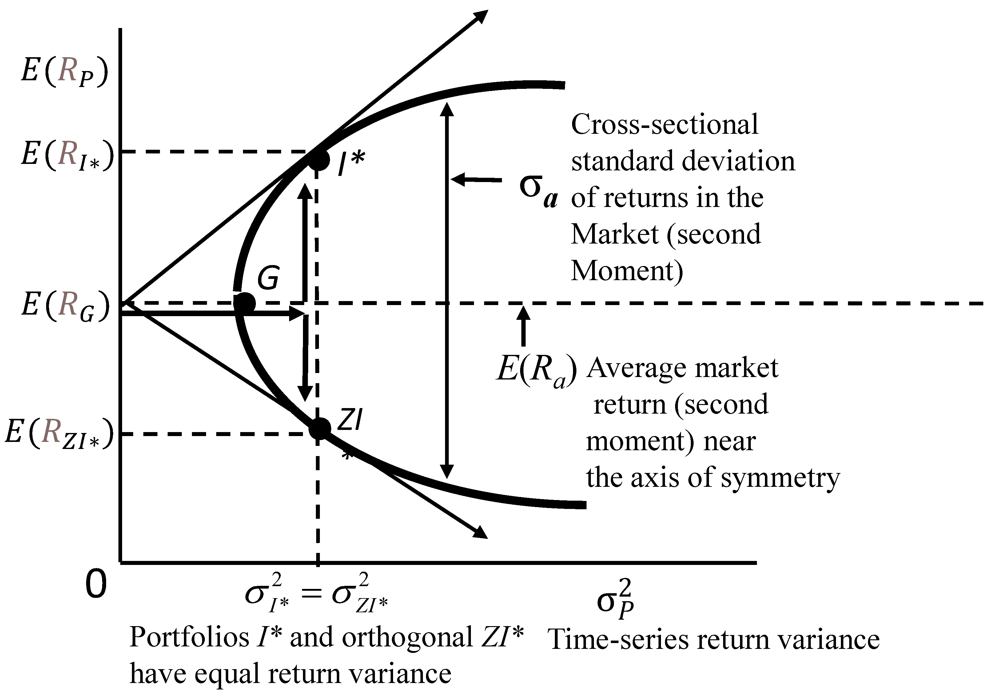
Figure 2.
Out-of-sample cross-sectional CAPM (Panel A) and Fama and French three-factor model (Panel B) mispricing errors comparing average one-month-ahead realized excess returns in percent (Y-axis) to average one-month-ahead predicted (fitted) excess returns in percent (X-axis) for 286 portfolios. The analysis period is July 1973 to December 2021.
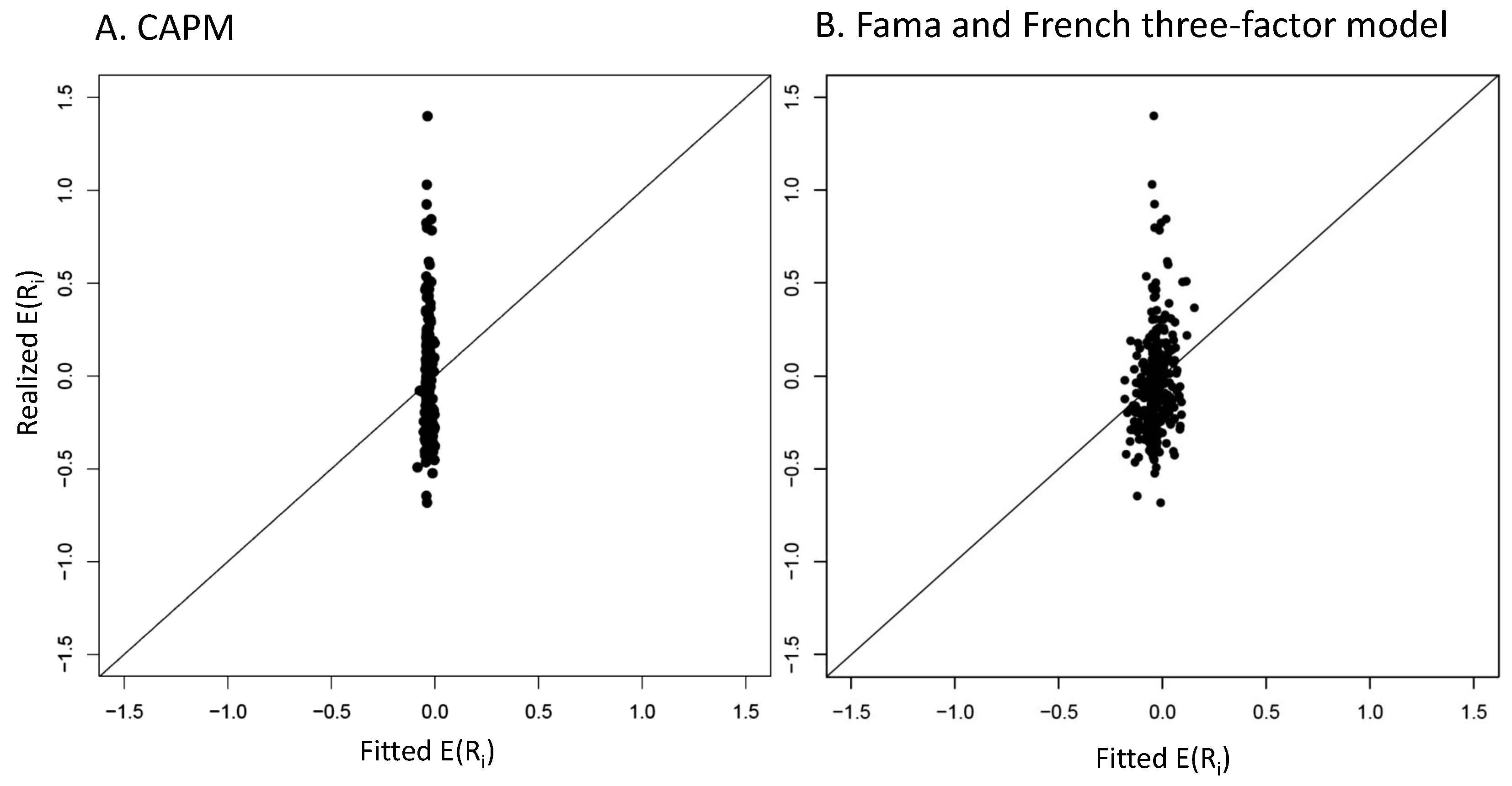
Figure 3.
Out-of-sample cross-sectional Carhart four-factor model (Panel A) and Fama and French five-factor model (Panel B) mispricing errors comparing average one-month-ahead realized excess returns in percent (Y-axis) to average one-month-ahead predicted (fitted) excess returns in percent (X-axis) for 286 portfolios. The analysis period is July 1973 to December 2021.
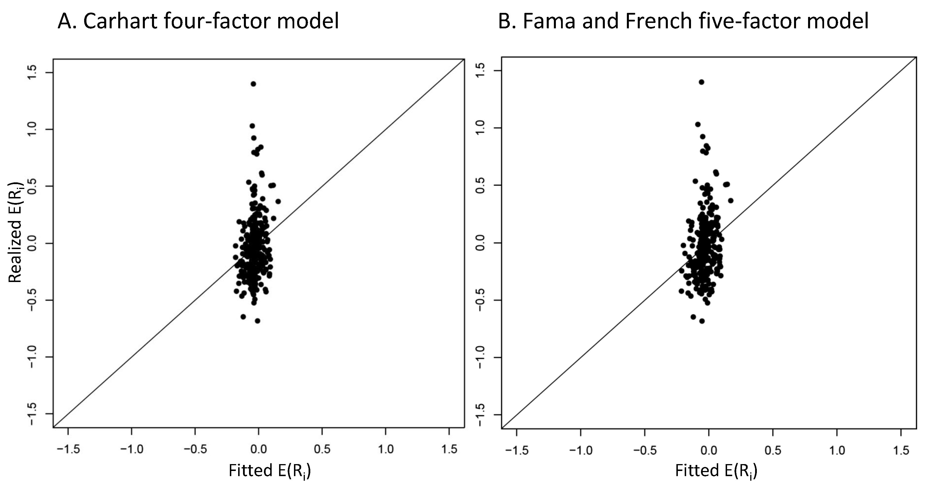
Figure 4.
Out-of-sample cross-sectional Fama and French six-factor model (Panel A) and ZCAPM (Panel B) mispricing errors comparing average one-month-ahead realized excess returns in percent (Y-axis) to average one-month-ahead predicted (fitted) excess returns in percent (X-axis) for 286 portfolios. The analysis period is July 1973 to December 2021.
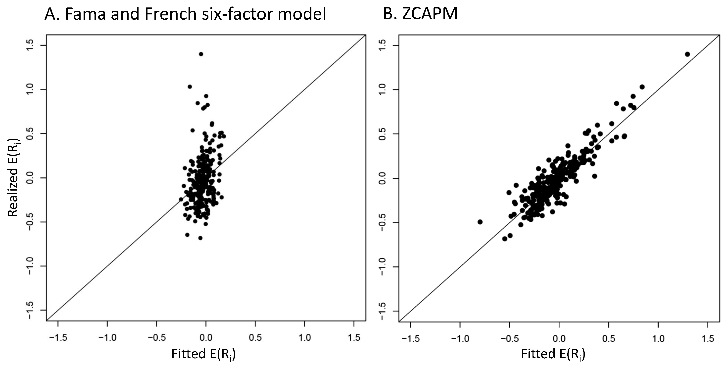
Table 1.
Descriptive statistics for asset pricing factors.
This table summarizes the descriptive statistics for the asset pricing factors. Distribution information is provided, including the mean return, standard deviation of returns, maximum and minimum returns, and 25th percentile (P25), median (P50), and 75th percentile (P75) returns. Daily factor returns (in percent) corresponding to different
asset pricing models are denoted as follows: (CRSP index return minus Treasury bill rate, see footnote 1), SMB (size), HML (value), MOM (momentum), RMW (profit), CMA (capital investment), and RD (market return dispersion), The sample period is from July 1972 to December 2021.
| Statistic | |||||||
|---|---|---|---|---|---|---|---|
| Mean | 0.01 | 0.005 | 0.01 | 0.03 | 0.01 | 0.01 | 1.86 |
| Standard deviation | 1.07 | 0.57 | 0.59 | 0.79 | 0.41 | 0.37 | 0.66 |
| Maximum | 11.35 | 6.17 | 6.74 | 7.12 | 4.52 | 2.53 | 10.77 |
| Minimum | -17.47 | -11.19 | -5.00 | -14.37 | -3.01 | -5.87 | 0.68 |
| P25 | -0.46 | -0.30 | -0.24 | -0.25 | -0.17 | -0.18 | 1.47 |
| P50 | 0.04 | 0.02 | 0.01 | 0.06 | 0.01 | 0.01 | 1.73 |
| P75 | 0.53 | 0.32 | 0.26 | 0.36 | 0.19 | 0.19 | 2.04 |
1 In the ZCAPM, due to using average market excess returns rather than a proxy for market portfolio excess returns, the market factor associated with CRSP index excess returns is denoted instead of per other models.
Table 2.
Out-of-sample Fama-MacBeth cross-sectional tests of 286 anomaly portfolios for asset pricing models in the sample period July 1972 to December 2021.
Using a total of 286 anomaly portfolios (comprised of 133 plus 153 anomalous portfolios from Chen and Zimmerman (2020) and Jensen, Kelly, and Pedersen (2023), respectively), this table contains results for the
full sample period July 1972 to December 2021. Based on standard two-step Fama-MacBeth cross-sectional tests, we report out-of-sample (one-month-ahead) estimated market prices of risk denoted for the kth factor for the analysis period July 1973 to December 2021. Associated t-statistics are shown in parentheses below estimated prices of risk. The asset pricing models are: CAPM, Fama and French three-factor model (FF3), Carhart four-factor model (C4), Fama and French five-factor model (FF5), Fama and French six-factor model (FF6), and ZCAPM. Factors in these models are denoted as m (CRSP index excess return, see footnote 1), RD (market return dispersion), SMB (size), HML (value), MOM (momentum), RMW (profit), and CMA (capital investment). Results are shown for the analysis period.
| Model | |||||||||
|---|---|---|---|---|---|---|---|---|---|
| CAPM | 0.44 | -0.00 | 0.01 | ||||||
| (17.77***) | (-0.01) | ||||||||
| FF3 | 0.42 | 0.07 | -0.09 | 0.27 | 0.11 | ||||
| (19.37***) | (0.39) | (-0.37) | (1.82*) | ||||||
| C4 | 0.40 | -0.04 | -0.13 | 0.26 | 0.31 | 0.17 | |||
| (18.52***) | (-0.23) | (-0.61) | (1.84*) | (1.29) | |||||
| FF5 | 0.40 | 0.12 | 0.04 | 0.12 | 0.18 | 0.32 | 0.15 | ||
| (20.33***) | (0.70) | (0.17) | (0.77) | (1.25) | (2.76***) | ||||
| FF6 | 0.38 | -0.04 | 0.03 | 0.18 | 0.40 | 0.19 | 0.26 | 0.19 | |
| (19.00***) | (-0.26) | (0.16) | (1.19) | (1.64) | (1.54) | (2.31**) | |||
| ZCAPM | 0.28 | 0.30 | 0.72 | 0.84 | |||||
| (9.96) | (1.43) | (6.69***) |
1 In the ZCAPM, due to using average market excess returns rather than a proxy for market portfolio excess returns, the price of beta risk associated with CRSP index excess returns is denoted instead of in the other models. Asterisks indicate the level of statistical significance: * – 10 percent, ** – 5 percent, and *** – 1 percent.
Disclaimer/Publisher’s Note: The statements, opinions and data contained in all publications are solely those of the individual author(s) and contributor(s) and not of MDPI and/or the editor(s). MDPI and/or the editor(s) disclaim responsibility for any injury to people or property resulting from any ideas, methods, instructions or products referred to in the content. |
© 2025 by the authors. Licensee MDPI, Basel, Switzerland. This article is an open access article distributed under the terms and conditions of the Creative Commons Attribution (CC BY) license (http://creativecommons.org/licenses/by/4.0/).
Copyright: This open access article is published under a Creative Commons CC BY 4.0 license, which permit the free download, distribution, and reuse, provided that the author and preprint are cited in any reuse.


