
Submitted:
17 April 2025
Posted:
18 April 2025
You are already at the latest version
Abstract
Advances in Machine Learning (ML) present new opportunities to systematically analyze the spatial complexity of urban form. This study presents a proof-of-concept for an interpretable methodological framework for clustering urban typologies. The methodology employs the Getis-Ord Gi* spatial autocorrelation metric as positional information to encourage the creation of spatially homogenous clusters. Clustering is performed using UMAP, a non-linear dimensionality reduction algorithm along with BIRCH, a scalable unsupervised clustering algorithm. The method utilizes 17 morphological indicators that capture urban form attributes at the block, plot and building scale. The proposed framework is pilot tested on the metropolitan area of Thessaloniki, Greece, revealing 14 distinct urban typologies that are organized into 5 families with similar characteristics. The typologies reveal, in an almost Conzenian fashion, patterns of urban development that are rooted in the city’s modern history. Results are validated both quantitatively with performance indicators and qualitatively using aerial imagery and established knowledge on Thessaloniki’s urban planning and evolution.
Keywords:
urban form
; urban morphology
; urban typology
; unsupervised clustering
; UMAP
; BIRCH
; machine learning
; spatial autocorrelation
; urban planning
1. Introduction
Urban typologies serve as an analytical lens through which we understand the spatial structure and the complex sociocultural, economic and environmental dimensions of urban landscapes [1]. The typological approach is historically rooted in qualitative studies whether perceptual-aesthetic [2,3], typo-morphological [4,5] or historico-geographical [6,7]. However, as Batty [8] argues, the scientific understanding of cities requires a shift towards quantitative methods of urban experimentation to validate prior empirical knowledge. This need has spurred a quantitative shift in urban analytics [9] and morphometrics [10] that is now being accelerated by advancements in Machine Learning (ML) and Artificial Intelligence (AI).
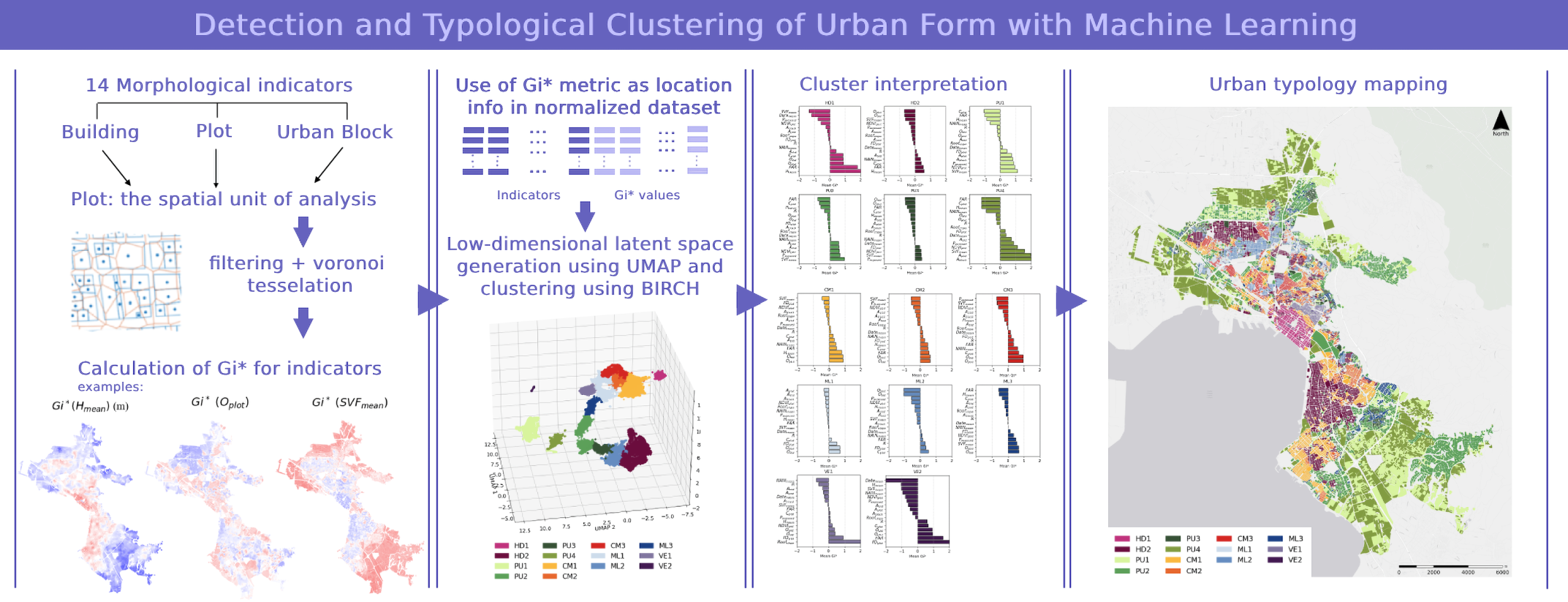
The present study contributes to the field of ML-driven urban analytics by developing and pilot-testing a scalable and interpretable method of unsupervised urban form typological clustering. The method innovates by integrating local spatial autocorrelation with two ML techniques: (i) Uniform Manifold Approximation and Projection (UMAP) for non-linear dimensionality reduction [11] and (ii) Balanced Iterative Reducing and Clustering using Hierarchies (BIRCH) for clustering [12]. The study employs the plot as the basic spatial unit, enabling significant analytical granularity while integrating land property geometry into the clustering process.
The method utilizes 17 morphological indicators at the building, plot and urban tissue scales, quantifying shape, orientation, density, openness, network integration and vegetation coverage. It is applied to the metropolitan area of Thessaloniki, Greece where over 85,000 plots are systematically analyzed and clustered. Results are validated ad-hoc using satellite images and findings from previous qualitative studies of its urban form. Although the method requires careful fine-tuning of model parameters, it manages to capture the variance of urban form, while remaining interpretable. Thus, the method has the capacity to provide quantitative insights to urban form evolution and ultimately inform urban planning, design and governance.
1.1. Clustering Urban Form with ML
Relatively recent reviews highlight the untapped potential of ML applications in morphological studies, including the clustering and classification of urban types [13,14]. Unsupervised clustering techniques like k-means, Gaussian Mixture Models (GMMs), Hierarchical Clustering and density-based methods like DBSCAN and HDBSCAN have been applied in urban form studies [15,16,17,18,19,20,21,22], albeit with limitations. For example, k-means assumes spherical equal-sized clusters [23], GMMs presuppose Gaussian distributions [24] while Hierarchical Clustering and DBSCAN do not scale well without optimizations [25,26]. HDBSCAN, while scalable and able to identify clusters of different shapes and sizes, may struggle with fuzzy cluster boundaries or homogenous densities [27].
Furthermore, all clustering algorithms become less effective for high-dimensional data due to the curse of dimensionality [28]. In such cases dimensionality reduction is often applied before clustering. Techniques include the Principal Component Analysis (PCA), t-SNE, UMAP and various Autoencoders based on Neural Network (NN) architectures [29,30]. PCA is quick, easy to use and interpretable, but can only perform linear reduction (ibid). t-SNE is geared towards 2D and 3D visualizations of non-linear relationships (ibid). Autoencoders, though powerful, require significant computational resources and time to design, optimize, train and validate while being notoriously harder to interpret (ibid).
To address these challenges, the study adopts an UMAP-BIRCH workflow. UMAP builds a fuzzy graph in high-dimensional space to encode relationships probabilistically and then creates a similar graph in low-dimensional (latent) space and aligns it with the original using gradient descent to preserve local and global structures [11]. BIRCH is then applied on the latent space. BIRCH excels in unsupervised clustering of big data with diverse cluster sizes and densities, using a Clustering Feature (CF) tree to organize data hierarchically and obtain more representative cluster centroids [12]. The proposed workflow excels at disentangling the complex, high-dimensional structure of urban form data while being relatively simple to implement and addressing computational and scalability challenges.
Additionally, the method needs to account for the spatial variability of urban form indicators which is crucial for detecting homogenous regions. Location in clustering and classification algorithms is often encoded using geographical coordinates, placenames, pixel coordinates (in the case of images) and graphs (if topology is important). Techniques such as spatially constrained clustering, graph-based clustering , Spatial Multiresolution Analysis (e.g., AMOEBA) [31,32,33] make use of such positional information. However, this study follows a different density-based approach where the relative concentration of similar values is considered more important than absolute location. This is achieved by calculating the Getis-Ord Gi* local spatial autocorrelation statistic for all indicators to guide clustering. This approach results in more homogenous clusters where hotspots and coldspots are detected.
1.2. The Plot as Elementary Spatial Unit
The selection of an elementary spatial unit is often determined by the scale and granularity of the typological study. Spatial units in previous studies range from entire cities [34] and districts [35] to urban blocks [36], plots [37] and finally buildings [38]. An alternative to using urban elements as geographical units is to apply spatial discretization methods, such as Voronoi tessellation from building footprints [15,39,40], gridding [18,41,42] or elastic urban “morpho-blocks” [43].
This study adopts the plot as the elementary spatial unit, as it represents the smallest cadastral subdivision of land and reflects an important interaction between land ownership and urban form. Plot configurations often reflect underlying socio-economic dynamics and historical circumstances, development pressures and formal urban planning processes, as well as adaptations to an ever-evolving urban landscape [5,44]. Moreover, plot boundaries are systematically surveyed and recorded in property management systems, making them geometrically and topologically reliable for subsequent quantitative studies.
Plots as elementary units, however, have caveats too. Firstly, they are not indivisible units of urban form [45]. A large plot, for example, may mask the internal heterogeneity of urban forms within it. Secondly, where land is communal or ownership is concentrated to very few public or private hands, the concept of the plot as a spatial unit loses its meaning. Finally, plots are topologically connected only to their immediate neighbors inside each block, which prevents more complex spatial calculations. For the above reasons the study proceeds by: (i) filtering out certain plot categories that do not fit the “conventional” definition of plot (e.g. streets and other large transportation infrastructure like railways and highways, forested lands, large public spaces, archaeological sites, active or ex-military installations, public utilities) and (ii) applying Voronoi tessellation using plot centroids (Figure 1). The latter creates a fully connected topology which is essential for correct calculation of spatial weights during autocorrelation.
1.3. Urban Form Indicators
Urban morphometrics utilize quantitative indicators that capture the spatial complexity of cities. These often describe gradients between polarities: compactness and openness, density and sprawl, order and entropy, centers and peripheries, perceptions of high or low quality and safety, the artificial and the natural [21,46,47,48,49,50]. Fleischmann et al. [15] provide a systematic classification of urban form indicators into six categories (dimension, shape, spatial distribution, intensity, connectivity and diversity) and three conceptual scales (small, medium, large). While research efforts push towards standardizing indicators for global applications [48], their selection ultimately depends on the study’s objective, the scale of analysis and geographic extents as well as the urban context and data availability.
The present study utilizes a set of 17 urban form indicators that span across all six suggested aforementioned categories. These are organized by urban element: (i) plot, (ii) building and (iii) urban tissue indicators (Table 1) and describe plot, building and urban block size, shape and orientation, vegetation and building coverage, openness and exposure of buildings and spaces, street network integration, building completion date and roof type.

Table 1.
Plot indicators.
| Plot Area (,in m²) | |
| Smaller plots are usually found in urban land, while larger plots are characteristic of peri-urban and special uses. Calculated from plot boundary vertices using Gauss’ formula (shoelace method) Σφάλμα! Το αρχείο προέλευσης της αναφοράς δεν βρέθηκε.). |
(1)where , coordinates of vertex i, n the number of plot vertices. |
| Rectangularity () | |
| Quantifies how closely the shape of a plot resembles a rectangle by comparing its area () to the area of its Minimum Bounding Rectangle (). A value of corresponds to perfect rectangle, indicating a formal plot subdivision process (2). | (2) |
| Plot Fractal Dimension () | |
| Captures the complexity of plot boundaries, reflecting how boundary length increases with area. For simple shapes, the fractal dimension approaches 1, while more complex boundaries yield higher values. A simplified calculation method is used here (3). | (3)where the plot perimeter |
| Normalized Plot Orientation () | |
| Differentiates between cardinally (Oplot ≈ 0) or intercardinally (Oplot ≈ 1) oriented plots. Cardinal orientations are associated with a street grid that runs along the North-South (N-S) and East-West (E-W) axes and intercardinal orientations with a NE-SW and SE-NW oriented grid (4). | (4)where is the azimuth of the longest side of the plot’s MBR, measured clockwise from true North. |
| Mean Plot NDVI (NDVIplot) | |
| Calculated via zonal statistics on plot features buffered at 10m to account for neighboring vegetation (e.g. street trees) Σφάλμα! Το αρχείο προέλευσης της αναφοράς δεν βρέθηκε.). | (5)where is the NDVI value of each pixel and the total number of pixels inside the buffered plot. |
Table 2.
Building indicators.
| Building footprint area (,in m²) | |
| Calculated from building footprint vertices using Gauss’ formula (shoelace method). | Same as Σφάλμα! Το αρχείο προέλευσης της αναφοράς δεν βρέθηκε.) (substituting ) |
| Mean Building Height () | |
| Calculated from an Urban Atlas + Global Human Settlements Layer building height composite raster using zonal statistics (6). | (6)where is the building height value of pixel belonging to the and is the total number of pixels within the . |
| Floor Area Ratio ( | |
| Calculated from plot geometries, building footprints and mean heights. Assumes a floor height of 3.5m (7). | (7)where is the mean floor height. |
| Plot Coverage (Cplot, in %) | |
| Measures the proportion of a plot occupied by building footprints. High coverage indicates dense urban development, while zero coverage vacant plots (8). | (8)where is the building footprint area. |
| Building Fractal Dimension () | |
| Similarly to , describes building shape complexity. | Same as (3) (substituting ) |
| Exposed perimeter ratio () | |
| The ratio of exposed building perimeter to total perimeter. Ranges from 0 to 1, with the former indicating a building whose walls fully attach to other buildings and the latter a fully detached building. Building envelope exposure is linked to energy performance and the urban microclimate (9). | (9)where is the building total perimeter length and the length of common boundaries with other buildings. |
| Normalized Building orientation () | |
| Differentiates between cardinally and intercardinally oriented buildings in the same way as does for plots. | Same as (4) (substitutes ) |
Table 3.
Urban tissue indicators.
| Urban Block Area (, m²) | |
| Smaller block sizes typically correspond to denser, more walkable urban cores or older urban tissues where historic development processes favored fine-grained subdivisions. Block area is passed to all plots that belong to each urban block. | Same as Σφάλμα! Το αρχείο προέλευσης της αναφοράς δεν βρέθηκε.) (substitutes ) |
| Mean building completion year ( | |
| Calculated from ELSTAT 2011 census data aggregated at the urban block scale and reported as number of buildings per time period (e.g. before 1919, 1919 - 1945, 1945-1960, 1960 - 1970... 2006 – 2011). is passed to all plots belonging to their respective urban block (10). | (10)where is the number of buildings erected during period , the median year of each period . |
| Sloped Roof Percentage per Urban Block () | |
| Calculated from ELSTAT 2011 census data aggregated at the urban block scale and reported as number of buildings per roof type. Most sloped roofs are tiled in the case study. is passed to all plots belonging to their respective urban block ( 11). | ( 11)where is the number of sloped roofs. |
| Mean Normalized Angular Integration () | |
| An important space syntax measure for assessing network integration [51]. Here local integration is calculated using a maximum radius of 200m to highlight local centers. Results are then interpolated with IDW to create a raster surface. Mean NAIN is calculated on plot geometries, buffered by 10m to account for proximity ( 12). | ( 12)where is a NAIN pixel value and the number of pixels within the plot buffer. |
| Mean Sky View Factor () | |
| Quantifies the proportion of sky visible from a given point. Values range from 0 (fully obstructed) to 1 (fully open). Influences daylighting, microclimate and perception of openness. Calculated using r.skyview on an urban DSM generated from building and terrain height data. Mean SVF is calculated on plot features and buffered by 10m ( 13). | ( 13)where the SVF value at each pixel and the number of pixels inside the buffered plot. |
1.4. The Study Area
The study focuses on the metropolitan area of Thessaloniki, Greece (φ=40°39’, λ=22°54’), a Mediterranean city with a well-documented history of urban transformations that encompasses several Municipalities (Figure 2). The city’s modern identity has largely been influenced by Ernest Hébrard’s plan after the great fire of 1917. It is considered as a remarkable case of early 20th century European urban planning that transformed the burned intra-muros city by introducing monumentalism in the form of emblematic axes, squares and vistas, while preserving important vernacular elements such as the “Ano Poli” (Upper City), the byzantine walls and the old city markets [52,53,54]. The city was also marked by the influx of Greek refugees from Minor Asia and later internal migration, dictating new urban extensions outside the historic center. Plans for new settlements and neighborhoods were hastily drafted and implemented to accommodate the fire victims and refugees. These often followed an undifferentiated grid pattern with little concern for existing landscape features and future growth demand.
Planning policies at the national and local level as well as socio-economic and cultural dynamics shaped the post-war urban fabric of Thessaloniki [55,56,57]. Housing demand in most cases was met by increasing permissible development without making the necessary adaptations to existing urban layouts and infrastructure. This issue was greater in areas developed before the 1980 planning reforms as plans were implemented in a fragmented and incremental manner. Before the reforms statutory planning had limited agency in plan implementation, plot readjustment and public lands acquisition.
These circumstances had a significant influence on the city’s character. Thessaloniki’s western neighborhoods faced significant challenges early on with informal housing, limited public spaces and higher FAR imposed on unsuitable urban layouts. In contrast, eastern neighborhoods like Karabournaki, Nea Krini and Ano Toumba witnessed densification from mid-1970’s onwards, allowing for plan revisions to partially adapt to increasing development pressures, while the upper economic classes were attracted mostly to eastern suburbs such as Pylaia, Thermi and Panorama. In the following decades the difference in environmental quality and density acted as a self-reinforcing mechanism of socioeconomic divide between a low and mid-income west and a mid to high-income east. Environmental studies highlight the lack of accessible green spaces [58,59], the worse air quality [60] and the higher Urban Heat Island (UHI) intensity in the western parts of the city [61].
Finally, since the 1990s most of Thessaloniki’s peri-urban area has been a transitional space of urban sprawl and “big-box developments” as agricultural land is being replaced by retail and office parks, logistics centers, light industries, education and research, tourism and entertainment.
2. Materials and Methods
The proposed methodological framework is outlined below:
- Pre-process data and calculate morphological indicators: As described in Section 1.3.
- Perform spatial autocorrelation: Use Voronoi tessellation to create a fully connected topology from plot centroids (Figure 1). Calculate Getis-Ord Gi* statistics to identify hotspots and coldspots.
- Prepare dataset for clustering: Merge morphological indicators and corresponding Gi* values into a unified datset. Normalize data in the (-1,1) range.
- Apply UMAP and BIRCH: Tune UMAP hyperparameters to encourage cluster formation and separation in latent space. Cluster the UMAP latent space using BIRCH.
- Clustering quality validation: Verify clustering separation, similarity and information loss using appropriate metrics.
- Visualize and interpret results: Map the cluster distributions, chart and analyze cluster characteristics. Perform ad-hoc validation of results with findings of prior qualitative studies.
The study employs several python libraries to achieve its goal, including OSMnx [62], Scikit-learn [63] and PySAL/ESDA [64]. NAIN calculation is performed using QGIS Depthmap plugin and depthmapXnet 0.35 [65]. SVF calculation is performed with GRASS r.skyview [66]. Data sources, accuracy and pre-processing steps are summarized in Table 4.
2.1. Indicator Overview
A first overview of the examined indicators is provided in the form of histograms (Figure 3) and the correlation matrix (Figure 4). Parameters like , , and exhibit highly skewed distributions and are shown in logarithmic scale (Figure 3). , and follow more gaussian distributions. In other indicators, the high frequency of extreme values often indicates a special condition. For example, a and a Cplot of zero or a near one indicate a vacant plot. In other cases, such as certain values may dominate the distribution. These outliers contain useful information for the clustering process and should not be discarded as “noise” or gross errors.
Regarding correlations between metrics (Figure 4), the strongest is observed between Oplot and Obld, indicating that building and plot orientations align for most of the dataset. SVFmean is strongly positively correlated with NDVIplot, Pexposed, moderately with Aplot and Ablock and strongly negatively correlated with Cplot and Hmean. These correlations are generally expected due to the urban-rural density gradient.
2.2. Spatial Autocorrelation
Global autocorrelation is performed calculating Moran’s I (14) and local via Getis-Ord Gi* statistics (15) [75]. Both require the calculation of spatial weights between each i,j point pair. The spatial weights matrix () was constructed using Queen contiguity, which defines neighbors based on shared borders or vertices. Row-normalization was then applied to standardize the influence of neighboring plots.
where n is the total number of spatial units, wij the spatial weights between locations i and j, yi, yj the values of the variable at i and j and the variable mean.
where , the variable’s mean and standard deviation respectively.
2.3. UMAP+BIRCH Clustering
UMAP is applied on a “global” dataset comprising the morphological indicators and their corresponding Gi* values. This allows clustering to equally consider information regarding the magnitude and the spatial concentration of indicators. The dataset is then normalized in the (-1,1) range to render data comparable to each other. UMAP has several key hyperparameters which are tuned according to Table 6. The selection of canberra distance as a distance metric is due to its sensitivity to differences in low-magnitude values. This is advantageous for clustering datasets where smaller values often carry significant discriminatory power and helps in cluster seperation [76]. Canberra distance is calculated as following:
where xi and yi are the values of the feature i for points x and y, and n is the total number of features.
The number of UMAP components (i.e. the latent space dimensions) is determined by the following criteria: (i) clustering is generally easier in low-dimensional spaces so the fewer the components the better, (ii) components should ideally be orthogonal to each other (i.e. independent), (iii) they should express complex data interactions that emerge within the dataset and (iv) the latent space should demonstrate separation of clusters.
Adherence to criteria (ii) and (iii) is estimated by calculating the correlations between components (Table 7, Table 8) and between each component and the 17 indicators (Figure 5). After several test-runs the number was fixed to 3 components: UMAP 1 describes “informality” or “vernacularity” as it indicates the complexity of plot and building shapes, building height and prevalence of sloped roofs, often associated with suburban or vernacular settings (Figure 5). UMAP 2 describes the “urbanization gradient”, that is mostly related to density-based indicators. Finally, UMAP 3 describes “directionality” as it is almost solely strongly related with both Oplot and Obld (Figure 5). For criterion (iv) it was found that the combination of canberra metric with increased “neighborhood size” and “negative sample rate” generates more separated and distinct regions in the latent space (Figure 6).
BIRCH is finally applied on UMAP components to cluster urban form types. BIRCH hyperparameters (Table 7) were selected to encourage splitting into smaller subclusters before the final agglomerative clustering step. For a threshold of 0.3, BIRCH generates 202 initial subclusters, which are further aggregated to 14 in the final clustering step. The number of final clusters is selected after several test-runs to strike balance between analytical granularity and interpretability, while monitoring cluster persistence in the resulting latent space (Figure 7).
2.4. Clustering Evaluation
Unsupervised clustering can be challenging to validate in absence of “ground truth” labelled data. The lack of labels means that clustering quality must be benchmarked indirectly, using performance metrics that evaluate aspects, such as cluster interpretability, cohesion and separation. This section compares three different scenarios to demonstrate methodological effectiveness: (i) clustering with Gi* values and selected UMAP+BIRCH hyperparameters, (ii) clustering without Gi* values and (iii) clustering with Gi* values and default hyperparameters. Three complementary metrics are employed to measure cluster quality: Silhouette Score [78], Jensen-Shannon (JS) Divergence [79], and Information Bottleneck Ratio (IBR) [80].
Silhouette score measures cluster cohesion in relation to distance from other clusters, with higher scores indicating better quality:
where : The average distance of point i to all other points in the same cluster and the average distance of point i to all points in the nearest neighboring cluster.
JS divergence quantifies cluster distinctness (or drift). It measures dissimilarity with zero indicating identical distributions:
where and : probability distributions (e.g., feature histograms of two clusters), their average, the Kullback-Leibler (KL) divergence: , which measures how much P differs from M. and the KL divergence for Q and M.
IBR measures information loss from the original dataset, with a value of one indicating no loss:
where the entropy of cluster k, calculated as: ( is the probability of point i in cluster k and is the number of points in cluster k) and the entropy of the entire dataset, calculated similarly to .
The calculated metrics for the three scenarios are shown in Table 9. The first scenario, which is what is applied in this study, achieves the best overall performance as it demonstrates a moderate Silhouette Score and higher JS-Divergence and IBR, indicating more distinct clusters and greater retention of information. Attempting clustering without Gi* values produces worse results, while using default hyperparameters yields even poorer clusters. It can be observed that even in the “best” case of scenario 1, clusters are not fully separated (as indicated by the Silhouette Score and visually confirmed by Figure 7.
What these metrics fail to describe is the cluster homogeneity in the actual geographical space. This can be confirmed visually by comparing the mapped clusters when Gi* values are used and when they aren’t. It can be seen (Figure 8) that the use of Gi* values indeed results in more spatially homogenous clusters.
3. Results
This section presents and analyses the 14 resulting clusters, which are organized into 5 families with similar characteristics (Table 10). The mean Gi* values are charted for each cluster (Figure 9 and Figure 10) to better understand the inter-cluster differences in spatial concentrations of the analyzed indicators. Finally, the resulting typological map (
Figure 11) is interpreted by aerial imagery of urban tissue samples (Appendix: Table) and findings from previous studies (Section 1.4).
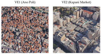
A first observation is that the method captures in an almost Conzenian fashion the patterns of urban form that have been the product of the case study city’s historical evolution. Cluster HD1 is exclusive to the “intra-muros” historic city center. Within it, cluster VE1 detects the vernacular “Ano Poli” and “Ladadika” districts and cluster VE2 the old city markets, which constitute important elements of the city’s urban heritage and identity. Cluster HD2 defines several high-density local centers outside the historic center that share similar morphological characteristics. Clusters PU1-4 describe peri-urban developments. PU1 focuses on vacant plots and lowrise detached buildings, PU2 and PU3 on suburbs with the latter having a more compact grid and smaller plots with less vegetation. PU4 is about industrial warehouses and newer “big-box” developments that continue to shape the peri-urban space since the 1990s.
Clusters CM1-3 describe mostly residential neighborhoods with midrises arranged in progressively denser configurations. An interesting observation is that CM1 covers mostly mid-income neighborhoods in both eastern and western Thessaloniki, while CM3 -the most compact variant- is almost exclusively found in western neighborhoods. Clusters ML1-3 describe mixes of midrise and lowrise buildings in different spatial arrangements. ML1 and ML2 are both exclusively found in western Thessaloniki. ML1 includes some of the poorest neighborhoods, such as “Dendropotamos”. ML2 is mostly found in the lower (Kato) Evosmos area and is characterized by narrow streets and minimal public spaces and vegetation. In contrast, ML3 is exclusive to eastern mid to high-income areas, such as “Konstantinoupolitika” and “Pylaia” with more openness and greenery.
The typology map (
Figure 11) highlights many of the old cores of neighborhoods outside the intra-muros city that were developed as a response to urgent historical needs for housing in the first half of the twentieth century. A tight, regular and undifferentiated grid is often the characteristic of the old cores of Efkarpia (PU3), Kordelio (HD2), Illioupoli (CM3), Ampelokipoi-Menemeni (CM3), Neapoli (HD2/ML2) Ano and Kato Toumba (CM1, CM2) and Kalamaria (CM1, HD2). While these areas belong to different clusters, their common characteristics make them stand out from the rest of the urban tissue. These findings are confirmed by historical aerial photographs (Figure 12) from the 1945-1960 dataset of the Hellenic Cadastre [81]. During the development boom of the 1960s and 1970s these older cores were eventually absorbed into the metropolitan urban tissue, yet the original grid and plot pattern is still evident today.
Overall, western Thessaloniki comprises a fragmented landscape of denser and in some cases chaotic urban typologies with little vegetation and open space (e.g. ML1, ML2, CM2). This is largely due to the lack of an overarching development vision and the limited role of statutory urban planning during a period of rapid post-war growth. This geographic distribution of typologies aligns with observations from previous studies on Thessaloniki’s urban form and socioeconomic discrepancies between lower to mid-income western neighborhoods and mid to high-income eastern neighborhoods (Section 1.4). It can only be hypothesized that over time urban form might have had a reinforcing effect in increasing these discrepancies.
4. Discussion
The results indicate that the selection of the plot as the basic spatial analysis unit was appropriate for the case study city. Yet, as the method was not tested in cities with non-plot-based urbanist traditions, the question of global applicability remains open. In an effort to address the shortcomings of the plot as a geographical unit, filtering and Voronoi tessellation had to be performed. It is likely that a more generalized approach will require a more robust form of spatial discretization, such as the “enclosed tessellation cells” suggested by Fleischmann and Arribas-Bel [45]. Another disadvantage of the proposed workflow is the difficulty in incorporating categorical data. A possible workaround might be the use of ensemble clustering, using different methods for categorical and numerical data.
The findings also support the idea of using the Gi* statistic to perform a more spatially aware clustering, leading to more spatially homogenous clusters. Many of the selected morphological indicators describe the variability of density across the urban-rural gradient (UMAP component 2), while they struggle to identify more complex spatial configurations, rhythms and patterns except for informality/vernacularity and grid directionality (components 1 and 3). It is also unclear whether different urban contexts might require a different set of indicators. Consequently, the question of indicator robustness also remains open. In any case, the proposed ML methodology is both modular and interpretable, enabling a greater degree of control of the process and its results, in contrast to more elaborate ML methods such as Deep Neural Networks.
While the method captures broad spatial patterns and some distinct micro-clusters, it also results in misidentifications. For example, the university campus and the HELEXPO convention center lie within the city center and contain some tall buildings, yet they are placed in the peri-urban family of clusters. This misclustering was persistent, irrespective of hyperparameter tuning during test-runs. The suburban cluster PU2 includes both the upper-class Panorama and areas of older informal development at the edge of Polichni. The monumental axis of Aristotelous Square is not detected. Cluster non-detection and misidentification can be attributed to several reasons such as: (i) limitations of selected morphological indicators, (ii) error propagation from utilized datasets, (iii) ecological fallacy where large plots may include more than one cluster of urban typologies and (iv) absence of pre-labeled data that might be used in a supervised or semi-supervised approach.
Despite these methodological shortcomings, an advantage of this method is the creation of a meaningful “latent space representation” of emergent urban form qualities via UMAP. There is no direct way to measure qualities such as “informality” or “urbanization”, yet a representation of these complex notions can be constructed from simpler morphometric indicators in a non-supervised manner as this study demonstrates. Perhaps future studies can expand upon this idea of latent representations of city form and function, to systematically analyze urban complexities.
5. Conclusions
This study presents a novel methodology for unsupervised urban typology clustering, integrating spatial autocorrelation and ML. The method utilizes UMAP for constructing a low-dimensional representation of 17 morphological indicators and their respective spatial concentration information in the form of Gi* values. Then BIRCH is applied on the compressed “latent space” to generate a map of 14 urban typologies. The methodology is applied to the metropolitan area of Thessaloniki, Greece. The study utilizes the plot as the fundamental spatial unit of analysis, employing appropriate filtering and Voronoi tessellation to partially address its shortcomings.
The resulting typological map reveals a hierarchy of urban forms that have evolved throughout the last century and until today under the influence of historic circumstances, regulatory frameworks, socio-economic forces and political decisions. The emergent clusters align and further verify quantitatively the key findings of previous qualitative studies of the city’s historic urban development and form. Methodologically, however, the chosen workflow is not an algorithmic panacea as questions remain open regarding the global applicability and the appropriateness of the plot as a spatial reference unit. These can be answered only within the scope of a broader study, as the current is limited to proof-of-concept.
Ultimately, the study invites reflection on both the potential and the limitations of data-driven urban morphometrics, especially in the case of unsupervised tasks. Informed use of the proposed methodological framework can deepen our understanding of urban form, as long as results are cross validated with prior knowledge obtained through qualitative methods. This limitation of the unsupervised approach underscores the need for a methodological paradigm shift -one that bridges the richness of qualitative urban form studies with the computational rigor of ML and AI.
Funding
This research received no external funding.
Data Availability Statement
All data sources and software used in the study are acknowledged in-text. Cadastral data used in the study are property of the Hellenic Cadastre and are available through its Open Data Portal (https://data.ktimatologio.gr/). For more information contact the author.
Conflicts of Interest
The authors declare no conflicts of interest.
Appendix A
Figure A1.
Hotspots and coldspots according to Gi* statistic.
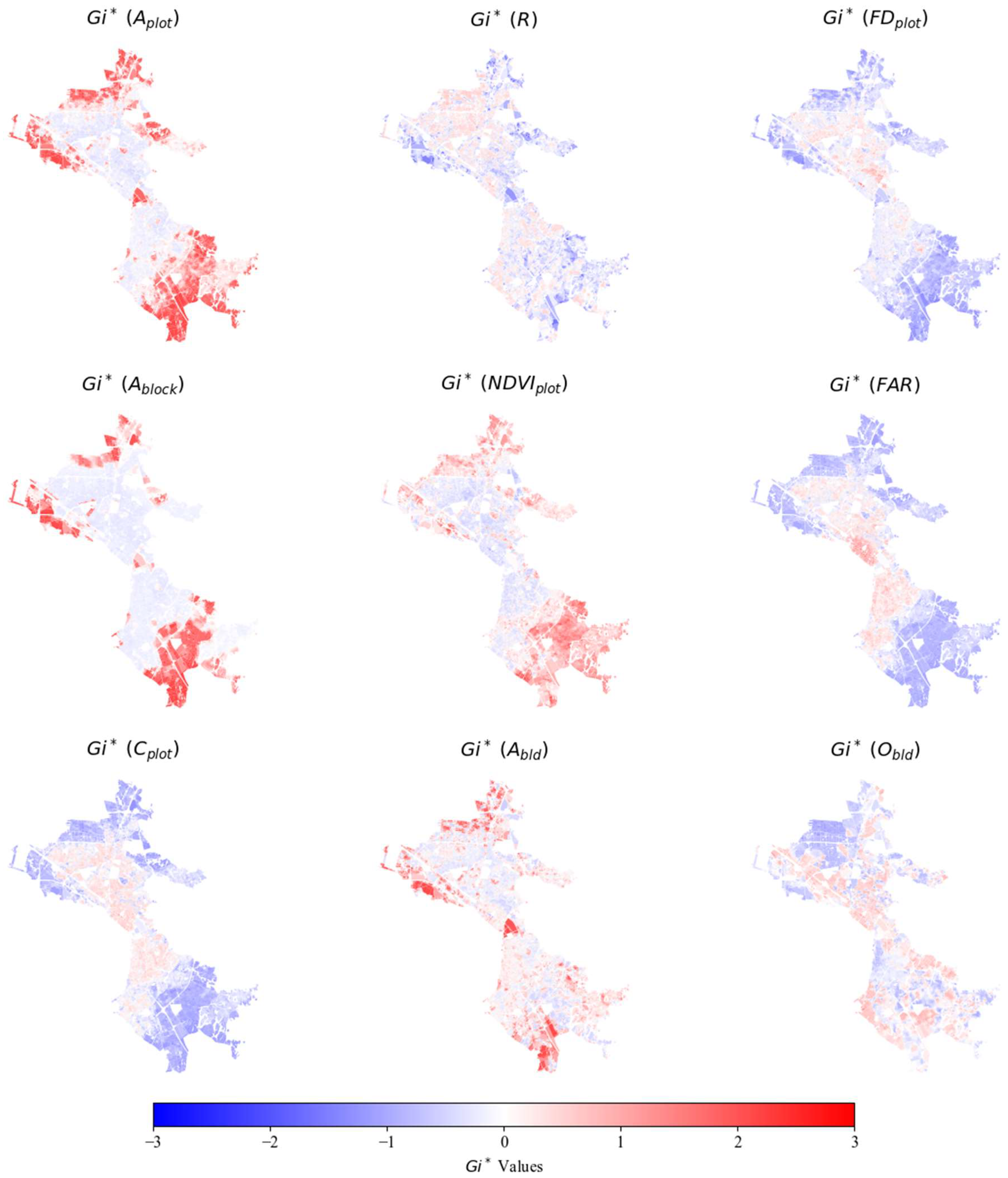
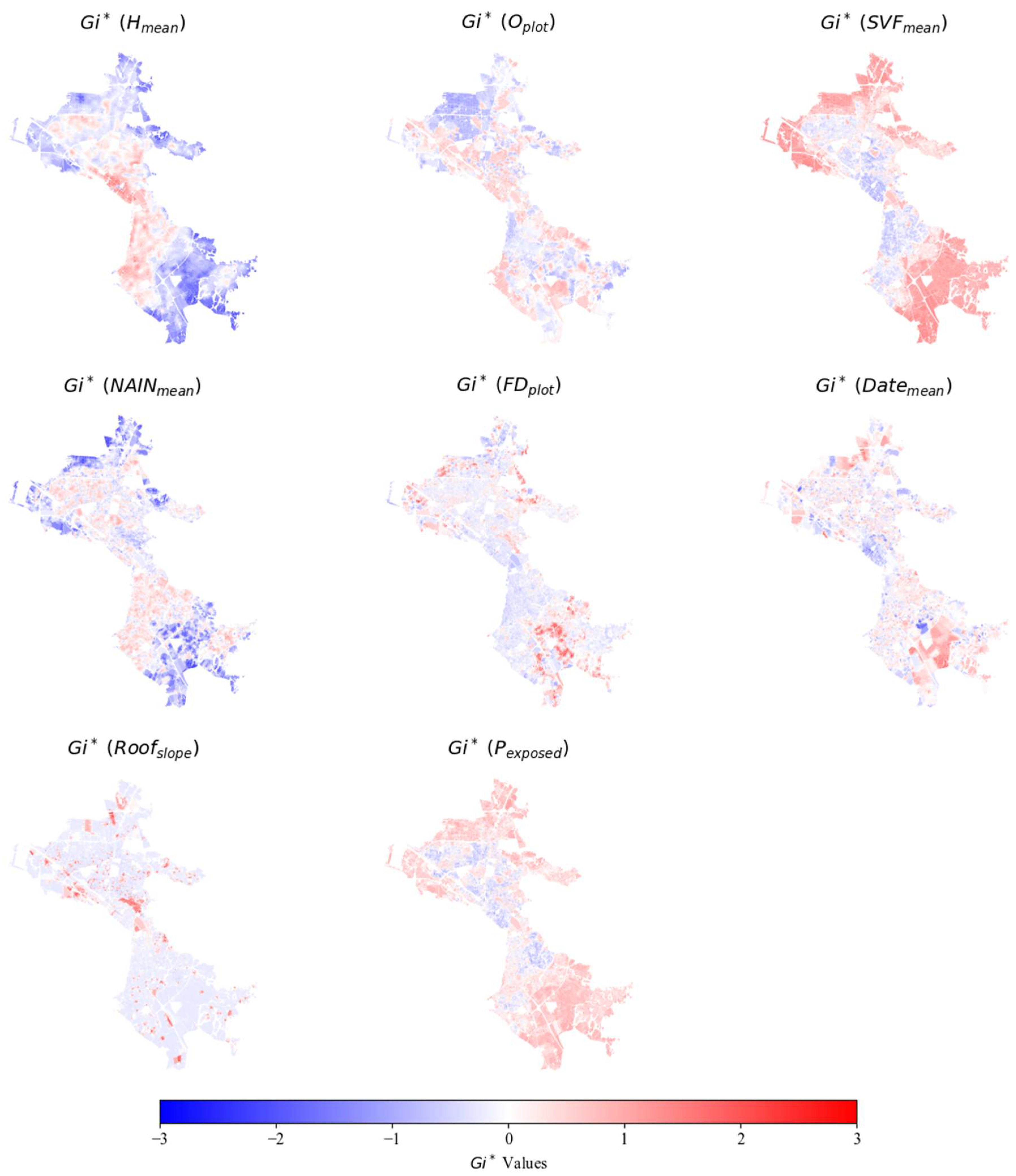
Figure A2.
Hotspots and coldspots according to Gi* statistic (continued).
Appendix B
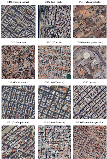
Table B1.
Examples of clustered urban form types [83].
Table B1.
Examples of clustered urban form types [83].
 |
 |
References
- Kropf, K. The Handbook of Urban Morphology; Wiley: Chichester, 2017. [Google Scholar]
- Camilo, S. City Planning According to Artistic Principles; Dover Publications: Dover, 1889. [Google Scholar]
- Cullen, G. Concise Townscape; Routledge: New York, 1961. [Google Scholar]
- Moudon, A.V. Getting to Know the Built Landscape: Typomorphology. In Ordering Space: Types in Architecture and Design; Franck, K.A., Schneekloth, L.H., Eds.; Van Nostrand Reinhold: New York, 1994; pp. 289–311. [Google Scholar]
- Panerai, P.; Castex, J.; Depaule, J.-C.; Samuels, I. Urban Forms: The Death and Life of the Urban Block; Routledge: New York, 2004; ISBN 978-0-7506-5607-8. [Google Scholar]
- Caniggia, G. Lettura Di Una Città: Como. 1963.
- Conzen, M.R.G. Thinking about Urban Form: Papers on Urban Morphology, 1932-1998; Peter Lang: Oxford, 2004; ISBN 978-3-03910-276-1. [Google Scholar]
- Batty, M. Science in Planning: Theory, Methods and Models. In Planning Knowledge and Research; Routledge, 2018 ISBN 978-1-315-30871-5.
- Batty, M. Urban Analytics Defined. Environment and Planning B: Urban Analytics and City Science 2019, 46, 403–405. [Google Scholar] [CrossRef]
- Dibble, J.; Prelorendjos, A.; Romice, O.; Zanella, M.; Strano, E.; Pagel, M.; Porta, S. On the Origin of Spaces: Morphometric Foundations of Urban Form Evolution. Environment and Planning B: Urban Analytics and City Science 2019, 46, 707–730. [Google Scholar] [CrossRef]
- McInnes, L.; Healy, J.; Melville, J. UMAP: Uniform Manifold Approximation and Projection for Dimension Reduction 2020.
- Zhang, T.; Ramakrishnan, R.; Livny, M. BIRCH: An Efficient Data Clustering Method for Very Large Databases. SIGMOD Rec. 1996, 25, 103–114. [Google Scholar] [CrossRef]
- Chaturvedi, V.; de Vries, W.T. Machine Learning Algorithms for Urban Land Use Planning: A Review. Urban Science 2021, 5, 68. [Google Scholar] [CrossRef]
- Wang, J.; Biljecki, F. Unsupervised Machine Learning in Urban Studies: A Systematic Review of Applications. Cities 2022, 129, 103925. [Google Scholar] [CrossRef]
- Fleischmann, M.; Romice, O.; Porta, S. Measuring Urban Form: Overcoming Terminological Inconsistencies for a Quantitative and Comprehensive Morphologic Analysis of Cities. Environment and Planning B: Urban Analytics and City Science 2021, 48, 2133–2150. [Google Scholar] [CrossRef]
- Iungman, T.; Khomenko, S.; Barboza, E.P.; Cirach, M.; Gonçalves, K.; Petrone, P.; Erbertseder, T.; Taubenböck, H.; Chakraborty, T.; Nieuwenhuijsen, M. The Impact of Urban Configuration Types on Urban Heat Islands, Air Pollution, CO2 Emissions, and Mortality in Europe: A Data Science Approach. The Lancet Planetary Health 2024, 8, e489–e505. [Google Scholar] [CrossRef]
- Jang, K.M.; Suh, H.; Haddad, F.G.; Sun, M.; Duarte, F.; Kim, Y. Urban Street Clusters: Unraveling the Associations of Street Characteristics on Urban Vibrancy Dynamics in Age, Time, and Day. Urban Info 2024, 3, 27. [Google Scholar] [CrossRef]
- Li, N.; Quan, S.J. Identifying Urban Form Typologies in Seoul Using a New Gaussian Mixture Model-Based Clustering Framework. Environment and Planning B: Urban Analytics and City Science 2023, 50, 2342–2358. [Google Scholar] [CrossRef]
- Oke, J.B.; Aboutaleb, Y.M.; Akkinepally, A.; Azevedo, C.L.; Han, Y.; Zegras, P.C.; Ferreira, J.; Ben-Akiva, M.E. A Novel Global Urban Typology Framework for Sustainable Mobility Futures. Environ. Res. Lett. 2019, 14, 095006. [Google Scholar] [CrossRef]
- Schmidt, V. Urban Morphology as a Key Parameter for Mitigating Urban Heat? – A Literature Review. IOP Conf. Ser.: Earth Environ. Sci. 2024, 1363, 012074. [Google Scholar] [CrossRef]
- Schwarz, N. Urban Form Revisited—Selecting Indicators for Characterising European Cities. Landscape and Urban Planning 2010, 96, 29–47. [Google Scholar] [CrossRef]
- Wu, C.; Wang, J.; Wang, M.; Kraak, M.-J. Machine Learning-Based Characterisation of Urban Morphology with the Street Pattern. Computers, Environment and Urban Systems 2024, 109, 102078. [Google Scholar] [CrossRef]
- He, H.; He, Y.; Wang, F.; Zhu, W. Improved K-Means Algorithm for Clustering Non-Spherical Data. Expert Systems 2022, 39, e13062. [Google Scholar] [CrossRef]
- Back, K.; Brown, D.P. Implied Probabilities in GMM Estimators. Econometrica 1993, 61, 971–975. [Google Scholar] [CrossRef]
- Sarma, A.; Goyal, P.; Kumari, S.; Wani, A.; Challa, J.S.; Islam, S.; Goyal, N. μDBSCAN: An Exact Scalable DBSCAN Algorithm for Big Data Exploiting Spatial Locality. In Proceedings of the 2019 IEEE International Conference on Cluster Computing (CLUSTER); September 2019; pp. 1–11. [Google Scholar]
- Sumengen, B.; Rajagopalan, A.; Citovsky, G.; Simcha, D.; Bachem, O.; Mitra, P.; Blasiak, S.; Liang, M.; Kumar, S. Scaling Hierarchical Agglomerative Clustering to Billion-Sized Datasets 2021.
- Malzer, C.; Baum, M. A Hybrid Approach To Hierarchical Density-Based Cluster Selection. In Proceedings of the 2020 IEEE International Conference on Multisensor Fusion and Integration for Intelligent Systems (MFI); September 14 2020; pp. 223–228. [Google Scholar]
- Peng, D.; Gui, Z.; Wu, H. Interpreting the Curse of Dimensionality from Distance Concentration and Manifold Effect 2024.
- Battey, C.J.; Coffing, G.C.; Kern, A.D. Visualizing Population Structure with Variational Autoencoders. G3 Genes|Genomes|Genetics 2021, 11, jkaa036. [Google Scholar] [CrossRef] [PubMed]
- Waggoner, P.D. Modern Dimension Reduction 2021.
- Duque, J.C.; Aldstadt, J.; Velasquez, E.; Franco, J.L.; Betancourt, A. A Computationally Efficient Method for Delineating Irregularly Shaped Spatial Clusters. J Geogr Syst 2011, 13, 355–372. [Google Scholar] [CrossRef]
- Kopczewska, K. Spatial Machine Learning: New Opportunities for Regional Science. Ann Reg Sci 2022, 68, 713–755. [Google Scholar] [CrossRef]
- Mondal, R.; Ignatova, E.; Walke, D.; Broneske, D.; Saake, G.; Heyer, R. Clustering Graph Data: The Roadmap to Spectral Techniques. Discov Artif Intell 2024, 4, 7. [Google Scholar] [CrossRef]
- Goerlich Gisbert, F.J.; Cantarino Martí, I.; Gielen, E. Clustering Cities through Urban Metrics Analysis. Journal of Urban Design 2017, 22, 689–708. [Google Scholar] [CrossRef]
- Ahn, H.; Lee, J.; Hong, A. Urban Form and Air Pollution: Clustering Patterns of Urban Form Factors Related to Particulate Matter in Seoul, Korea. Sustainable Cities and Society 2022, 81, 103859. [Google Scholar] [CrossRef]
- Joshi, M.Y.; Rodler, A.; Musy, M.; Guernouti, S.; Cools, M.; Teller, J. Identifying Urban Morphological Archetypes for Microclimate Studies Using a Clustering Approach. Building and Environment 2022, 224, 109574. [Google Scholar] [CrossRef]
- Bobkova, E.; Berghauser Pont, M.; Marcus, L. Towards Analytical Typologies of Plot Systems: Quantitative Profile of Five European Cities. Environment and Planning B: Urban Analytics and City Science 2021, 48, 604–620. [Google Scholar] [CrossRef]
- Li, X.; Yao, R.; Liu, M.; Costanzo, V.; Yu, W.; Wang, W.; Short, A.; Li, B. Developing Urban Residential Reference Buildings Using Clustering Analysis of Satellite Images. Energy and Buildings 2018, 169, 417–429. [Google Scholar] [CrossRef]
- Porta, S.; Venerandi, A.; Feliciotti, A.; Raman, S.; Romice, O.; Wang, J.; Kuffer, M. Urban MorphoMetrics + Earth Observation: An Integrated Approach to Rich/Extra-Large-Scale Taxonomies of Urban Form. Projections, T: Measuring the City.
- Schirmer, P.M.; Axhausen, K.W. Axhausen, K.W. A Multiscale Clustering of the Urban Morphology for Use in Quantitative Models. In The Mathematics of Urban Morphology; D’Acci, L., Ed.; Springer International Publishing: Cham, 2019; ISBN 978-3-030-12381-9. [Google Scholar]
- Li, J.; Li, C. Characterizing Urban Spatial Structure through Built Form Typologies: A New Framework Using Clustering Ensembles. Land Use Policy 2024, 141, 107166. [Google Scholar] [CrossRef]
- Musiaka, Ł.; Nalej, M. Application of GIS Tools in the Measurement Analysis of Urban Spatial Layouts Using the Square Grid Method. ISPRS International Journal of Geo-Information 2021, 10, 558. [Google Scholar] [CrossRef]
- Ma, R.; Li, X.; Chen, J. An Elastic Urban Morpho-Blocks (EUM) Modeling Method for Urban Building Morphological Analysis and Feature Clustering. Building and Environment 2021, 192, 107646. [Google Scholar] [CrossRef]
- Porta, S.; Romice, O. Plot-Based Urbanism: Towards Time-Consciousness in Place-Making; University of Strathclyde - Urban Design Studies Unit: Strathclyde, 2010. [Google Scholar]
- Fleischmann, M.; Arribas-Bel, D. Geographical Characterisation of British Urban Form and Function Using the Spatial Signatures Framework. Scientific Data 2022, 9, 546. [Google Scholar] [CrossRef]
- Adolphe, L. A Simplified Model of Urban Morphology: Application to an Analysis of the Environmental Performance of Cities. Environment and Planning B: Planning and Design 2001, 28, 183–200. [Google Scholar] [CrossRef]
- Boeing, G.; Higgs, C.; Liu, S.; Giles-Corti, B.; Sallis, J.F.; Cerin, E.; Lowe, M.; Adlakha, D.; Hinckson, E.; Moudon, A.V.; et al. Using Open Data and Open-Source Software to Develop Spatial Indicators of Urban Design and Transport Features for Achieving Healthy and Sustainable Cities. The Lancet Global Health 2022, 10, e907–e918. [Google Scholar] [CrossRef]
- Clifton, K.; Ewing, R.; Knaap, G.; Song, Y. Quantitative Analysis of Urban Form: A Multidisciplinary Review. Journal of Urbanism: International Research on Placemaking and Urban Sustainability 2008, 1, 17–45. [Google Scholar] [CrossRef]
- Hou, Y.; Quintana, M.; Khomiakov, M.; Yap, W.; Ouyang, J.; Ito, K.; Wang, Z.; Zhao, T.; Biljecki, F. Global Streetscapes — A Comprehensive Dataset of 10 Million Street-Level Images across 688 Cities for Urban Science and Analytics. ISPRS Journal of Photogrammetry and Remote Sensing 2024, 215, 216–238. [Google Scholar] [CrossRef]
- Zhang, P.; Ghosh, D.; Park, S. Spatial Measures and Methods in Sustainable Urban Morphology: A Systematic Review. Landscape and Urban Planning 2023, 237, 104776. [Google Scholar] [CrossRef]
- Van Nes, A.; Yamu, C. Introduction to Space Syntax in Urban Studies; Springer International Publishing: Cham, 2021; ISBN 978-3-030-59139-7. [Google Scholar]
- Kalogirou, N. The Palimpsest of Aristotelous: Byzantine visions and eclectic localism; University Studio Press: Thessaloniki, 2021. [Google Scholar]
- Lagopoulos, A.Ph. Monumental Urban Space and National Identity: The Early Twentieth Century New Plan of Thessaloniki. Journal of Historical Geography 2005, 31, 61–77. [Google Scholar] [CrossRef]
- Yerolympos, A. Thessaloniki (Salonika) before and after 1917. Twentieth Century Planning versus 20 Centuries of Urban Evolution. Planning Perspectives 1988, 3, 141–166. [Google Scholar] [CrossRef]
- Bastéa, E.; Hastaoglou-Martinidis, V. Urban Change and the Persistence of Memory in Modern Thessaloniki. In Thessaloniki; Routledge, 2020 ISBN 978-0-429-20156-1.
- Gemenetzi, G. Thessaloniki: The Changing Geography of the City and the Role of Spatial Planning. Cities 2017, 64, 88–97. [Google Scholar] [CrossRef]
- Oikonomou, M.; Christodoulou, C. Evolution and Transformation Processes of Urban Form: Urban Tissues in Thessaloniki, Greece. In Proceedings of the Conference Proceedings – XXIX International Seminar on Urban Form ISUF 2022: Urban Redevelopment and Revitalisation. A Multidisciplinary Perspective; Lodz University of Technology Press; 2022. [Google Scholar]
- Karagianni, M. Making Thessaloniki Resilient? The Enclosing Process of the Urban Green Commons. UP 2022, 8. [Google Scholar] [CrossRef]
- Latinopoulos, D. Evaluating the Importance of Urban Green Spaces: A Spatial Analysis of Citizens’ Perceptions in Thessaloniki. Euro-Mediterr J Environ Integr 2022, 7, 299–308. [Google Scholar] [CrossRef]
- Moussiopoulos, Ν.; Vlachokostas, Ch.; Tsilingiridis, G.; Douros, I.; Hourdakis, E.; Naneris, C.; Sidiropoulos, C. Air Quality Status in Greater Thessaloniki Area and the Emission Reductions Needed for Attaining the EU Air Quality Legislation. Science of The Total Environment 2009, 407, 1268–1285. [Google Scholar] [CrossRef]
- Giannaros, T.M.; Melas, D. Study of the Urban Heat Island in a Coastal Mediterranean City: The Case Study of Thessaloniki, Greece. Atmospheric Research 2012, 118, 103–120. [Google Scholar] [CrossRef]
- Boeing, G. OSMnx: New Methods for Acquiring, Constructing, Analyzing, and Visualizing Complex Street Networks. Computers, Environment and Urban Systems 2017, 65, 126–139. [Google Scholar] [CrossRef]
- Scikit-learn Scikit-Learn: Machine Learning in Python Available online:. Available online: https://scikit-learn.org/stable/index.html (accessed on 19 January 2025).
- Rey, S.J.; Anselin, L. PySAL: A Python Library of Spatial Analytical Methods. In Handbook of Applied Spatial Analysis: Software Tools, Methods. In Handbook of Applied Spatial Analysis: Software Tools, Methods and Applications; Fischer, M.M., Getis, A., Eds.; Springer: Berlin, Heidelberg, 2010; ISBN 978-3-642-03647-7. [Google Scholar]
- Varoudis, T. depthmapX 2025.
- Zakšek, K.; Oštir, K.; Kokalj, Ž. Sky-View Factor as a Relief Visualization Technique. Remote Sensing 2011, 3, 398–415. [Google Scholar] [CrossRef]
- HC Download Service (WFS) for the Land Plots of the Public Legal Entity “Hellenic Cadastre” Available online:. Available online: https://data.ktimatologio.gr/dataset/27a9e70e-5232-485d-b407-c89e9d45c6b6 (accessed on 19 January 2025).
- EC Normalised Difference Vegetation Index 2016-Present (Raster 10 m), Europe, Daily Available online:. Available online: https://land.copernicus.eu/en/products/vegetation/high-resolution-normalised-difference-vegetation-index (accessed on 19 January 2025).
- OpenStreetMap OpenStreetMap Available online:. Available online: http://www.openstreetmap.org/ (accessed on 10 November 2024).
- El-Ashmawy, K.L.A. Testing the Positional Accuracy of OpenStreetMap Data for Mapping Applications. Geodesy and Cartography 2016, 42, 25–30. [Google Scholar] [CrossRef]
- EEA Copernicus Land Monitoring Service - Urban Atlas Available online: ea.europa.eu/data-and-maps/data/copernicus-land-monitoring-service-urban-atla (accessed on 16 February 2018).
- EC GHSL Data Package R2023 Available online:. Available online: https://human-settlement.emergency.copernicus.eu/ (accessed on 19 January 2025).
- EEA European Digital Elevation Model (EU-DEM) Available online:. Available online: https://www.eea.europa.eu/en/datahub/datahubitem-view/d08852bc-7b5f-4835-a776-08362e2fbf4b (accessed on 19 January 2025).
- ELSTAT ELSTAT 2011 Census data 2011.
- Getis, A. Spatial Autocorrelation. In Handbook of Applied Spatial Analysis: Software Tools, Methods and Applications; Fischer, M.M., Getis, A., Eds.; Springer: Berlin, Heidelberg, 2010; ISBN 978-3-642-03647-7. [Google Scholar]
- Yang, Y.; Sun, H.; Zhang, Y.; Zhang, T.; Gong, J.; Wei, Y.; Duan, Y.-G.; Shu, M.; Yang, Y.; Wu, D.; et al. Dimensionality Reduction by UMAP Reinforces Sample Heterogeneity Analysis in Bulk Transcriptomic Data. Cell Reports 2021, 36. [Google Scholar] [CrossRef]
- McInnes, L. UMAP: Uniform Manifold Approximation and Projection for Dimension Reduction — Umap 0. Available online: https://umap-learn.readthedocs.io/en/latest/ (accessed on 20 January 2025).
- Rousseeuw, P.J. Silhouettes: A Graphical Aid to the Interpretation and Validation of Cluster Analysis. Journal of Computational and Applied Mathematics 1987, 20, 53–65. [Google Scholar] [CrossRef]
- Nielsen, F. On the Jensen-Shannon Symmetrization of Distances Relying on Abstract Means. Entropy (Basel) 2019, 21. [Google Scholar] [CrossRef]
- Tishby, N.; Pereira, F.C.; Bialek, W. The Information Bottleneck Method 2000.
- Hellenic Cadastre Aerial Photos Viewing Service Available online: http://gis.ktimanet.gr/wms/ktbasemap/default.aspx.
- Esri; DeLorme; NAVTEQ Light Gray Canvas Base Available online: https://www.arcgis.com/home/item.html?id=291da5eab3a0412593b66d384379f89f.
- Google Google Earth Available online: https://www.google.com/earth.
Figure 1.
Example of Voronoi tessellation using plot centroids.

Figure 2.
Map of Municipality borders and mentioned placenames. Municipalities here correspond to the previous system of local governance as their borders match the extent of the metropolitan area more closely.
Figure 2.
Map of Municipality borders and mentioned placenames. Municipalities here correspond to the previous system of local governance as their borders match the extent of the metropolitan area more closely.
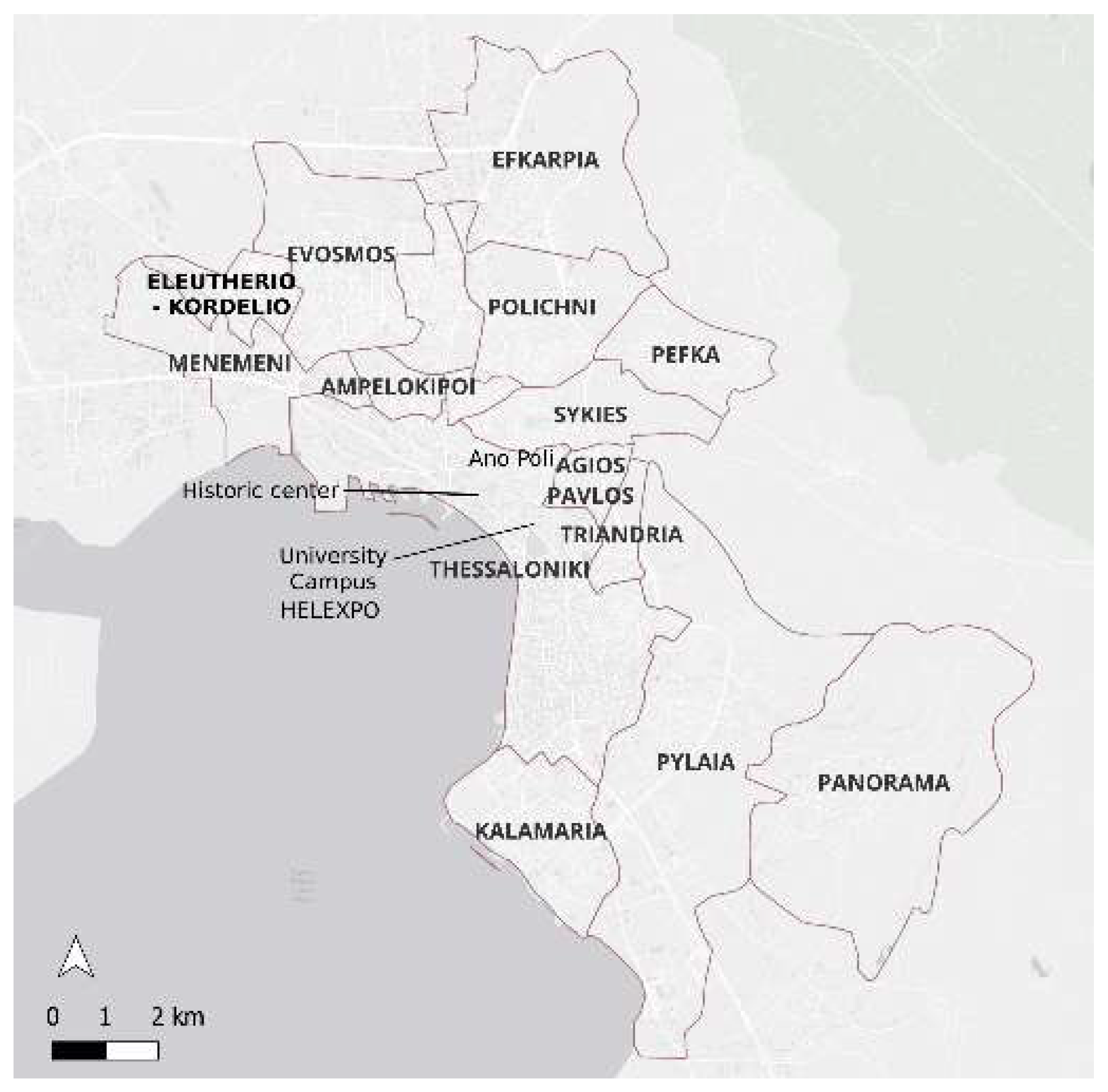
Figure 3.
Histograms of the pre-processed indicators.
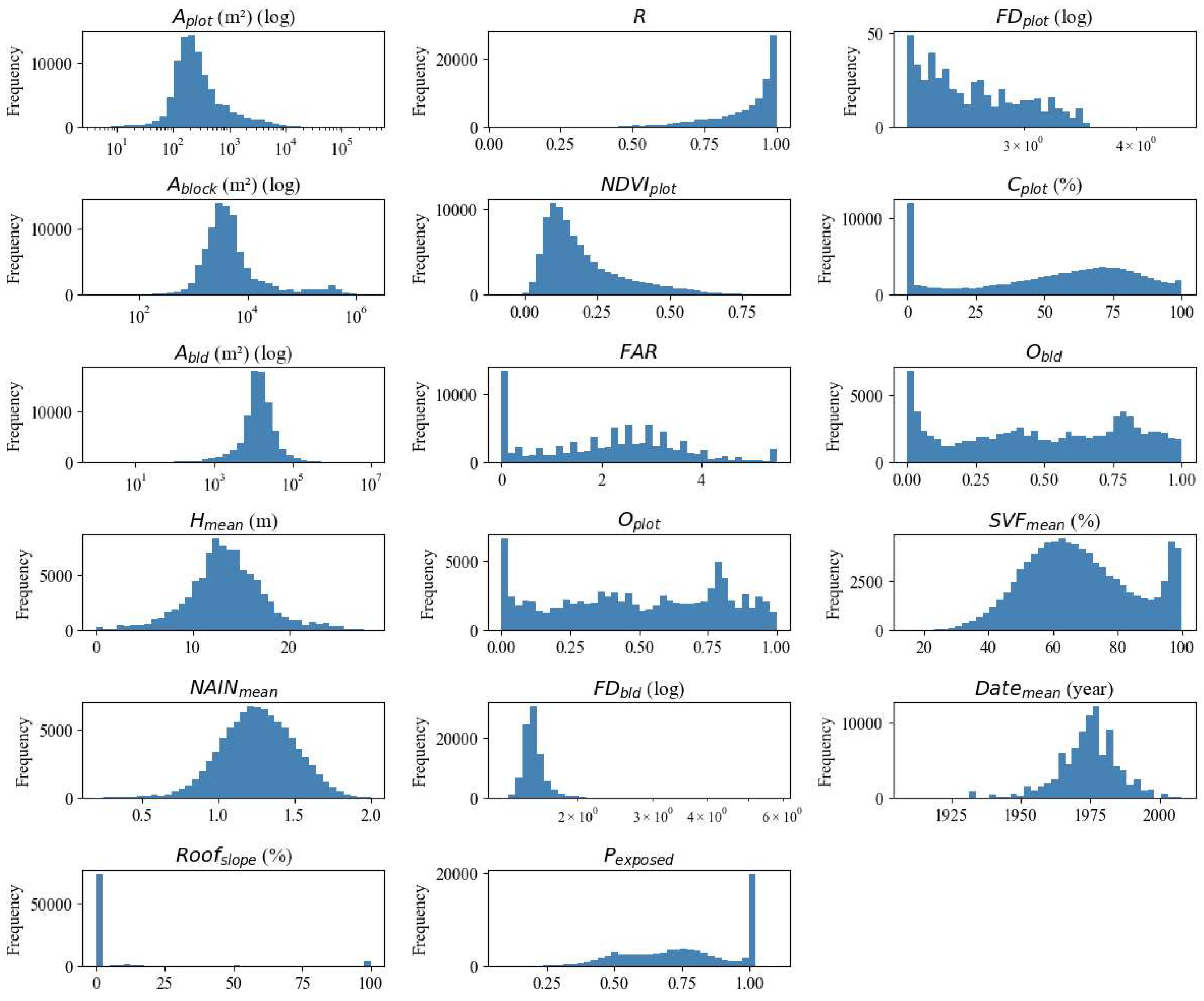
Figure 4.
Correlation matrix for the morphological indicators.
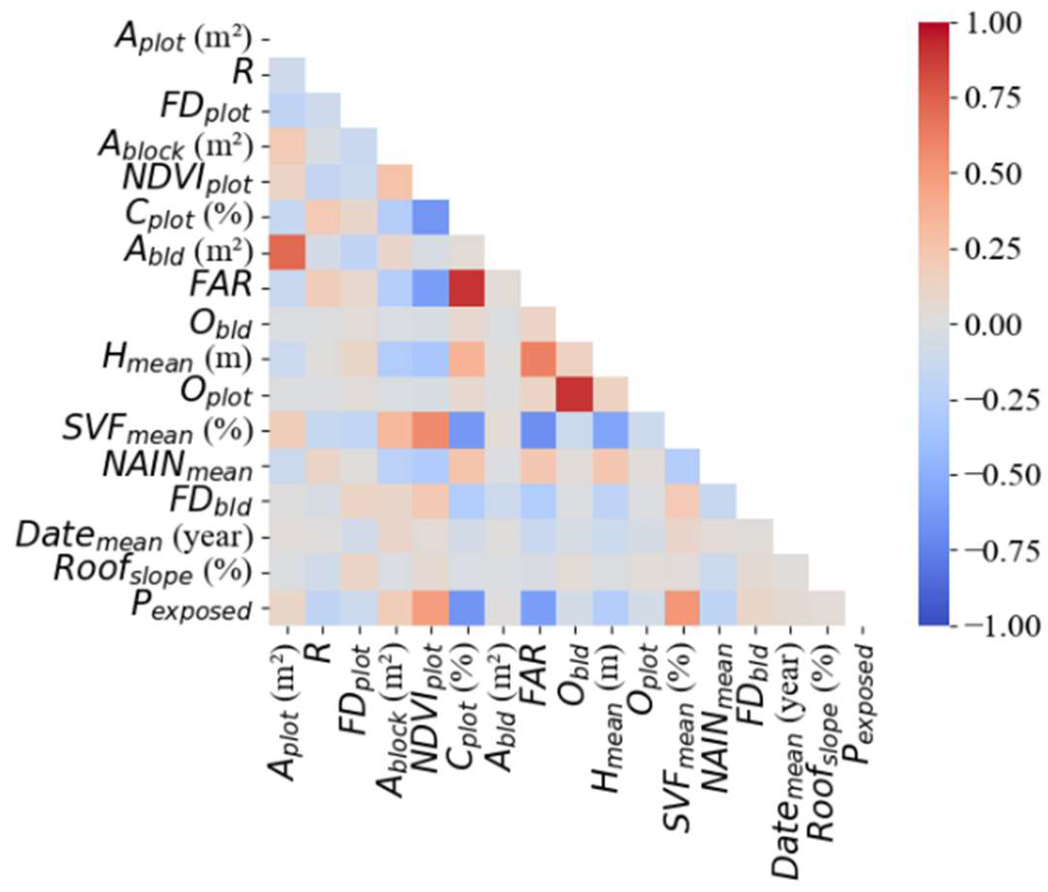
Figure 5.
Morphological indicators and UMAP components correlation matrix.
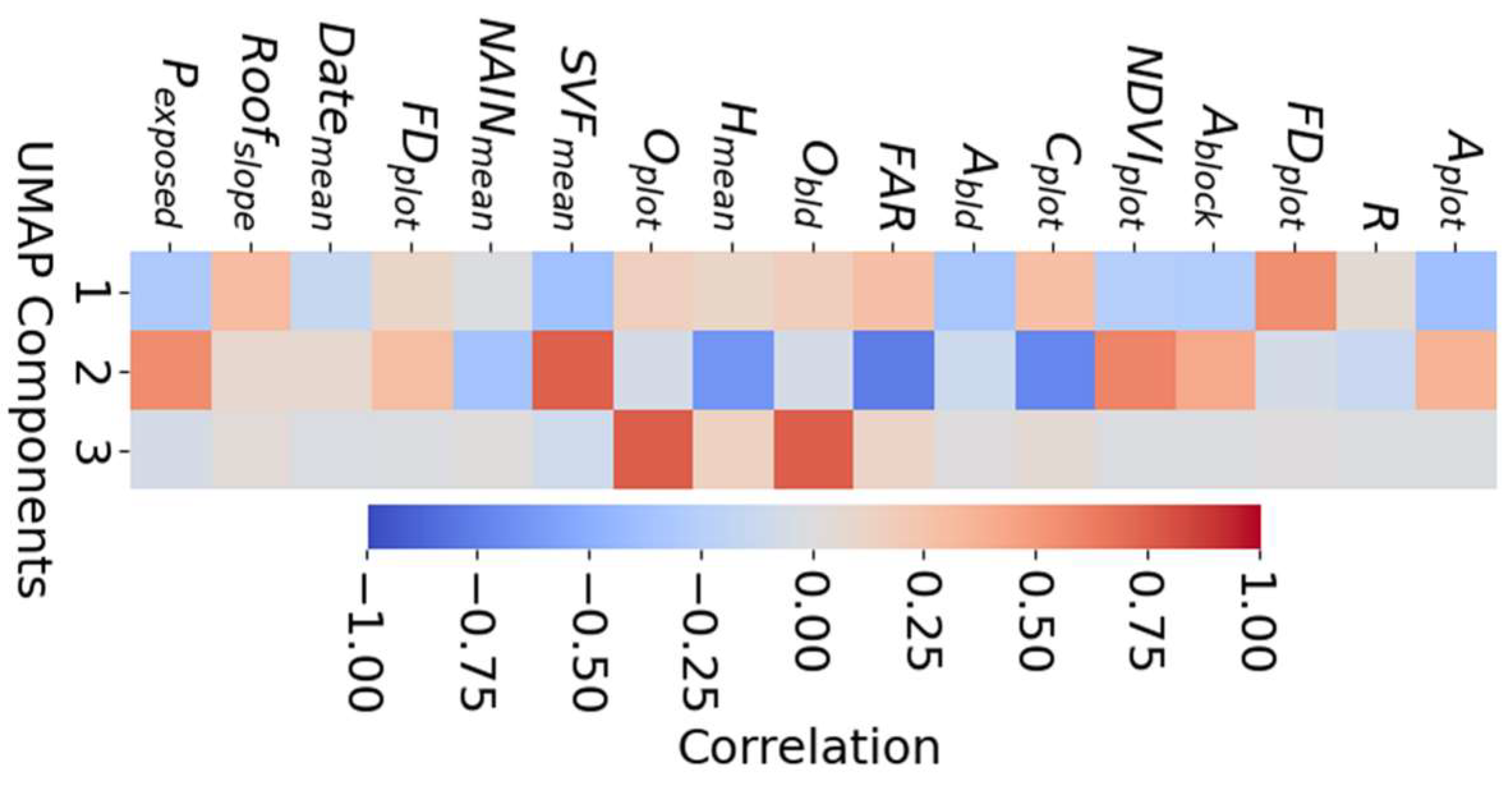
Figure 6.
Spatial distribution of UMAP components.
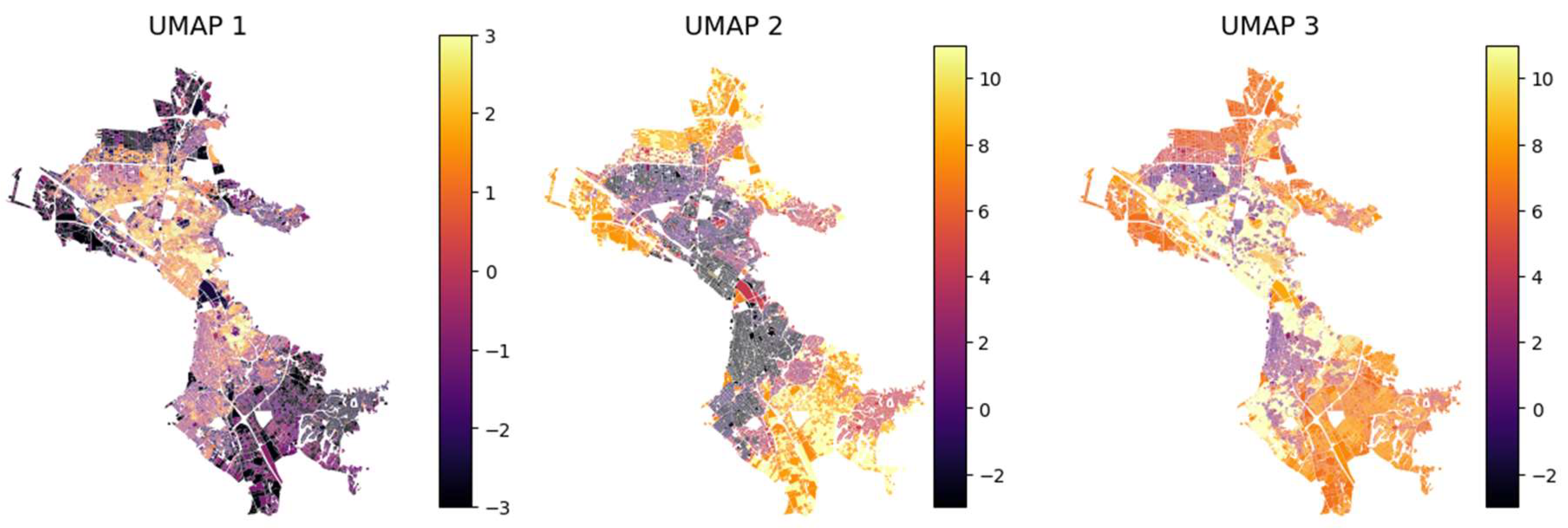
Figure 7.
Birch Clusters in UMAP Latent Space. Cluster coloring and coding is explained in the Results section.
Figure 7.
Birch Clusters in UMAP Latent Space. Cluster coloring and coding is explained in the Results section.
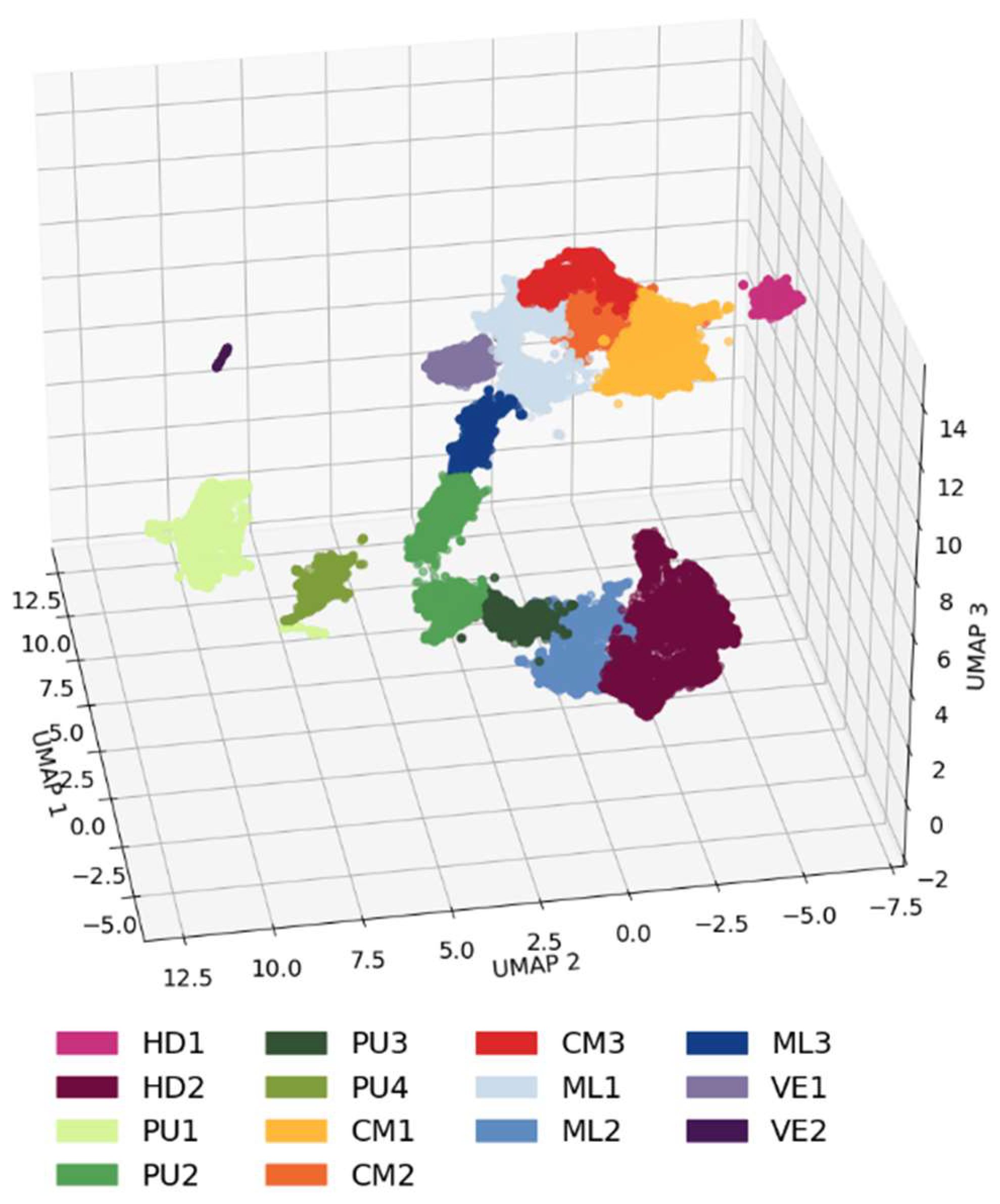
Figure 8.
Differences in cluster geographical homogeneity when Gi* values are included in the dataset (left) and when they are not (right). Cluster colors are randomized.
Figure 8.
Differences in cluster geographical homogeneity when Gi* values are included in the dataset (left) and when they are not (right). Cluster colors are randomized.
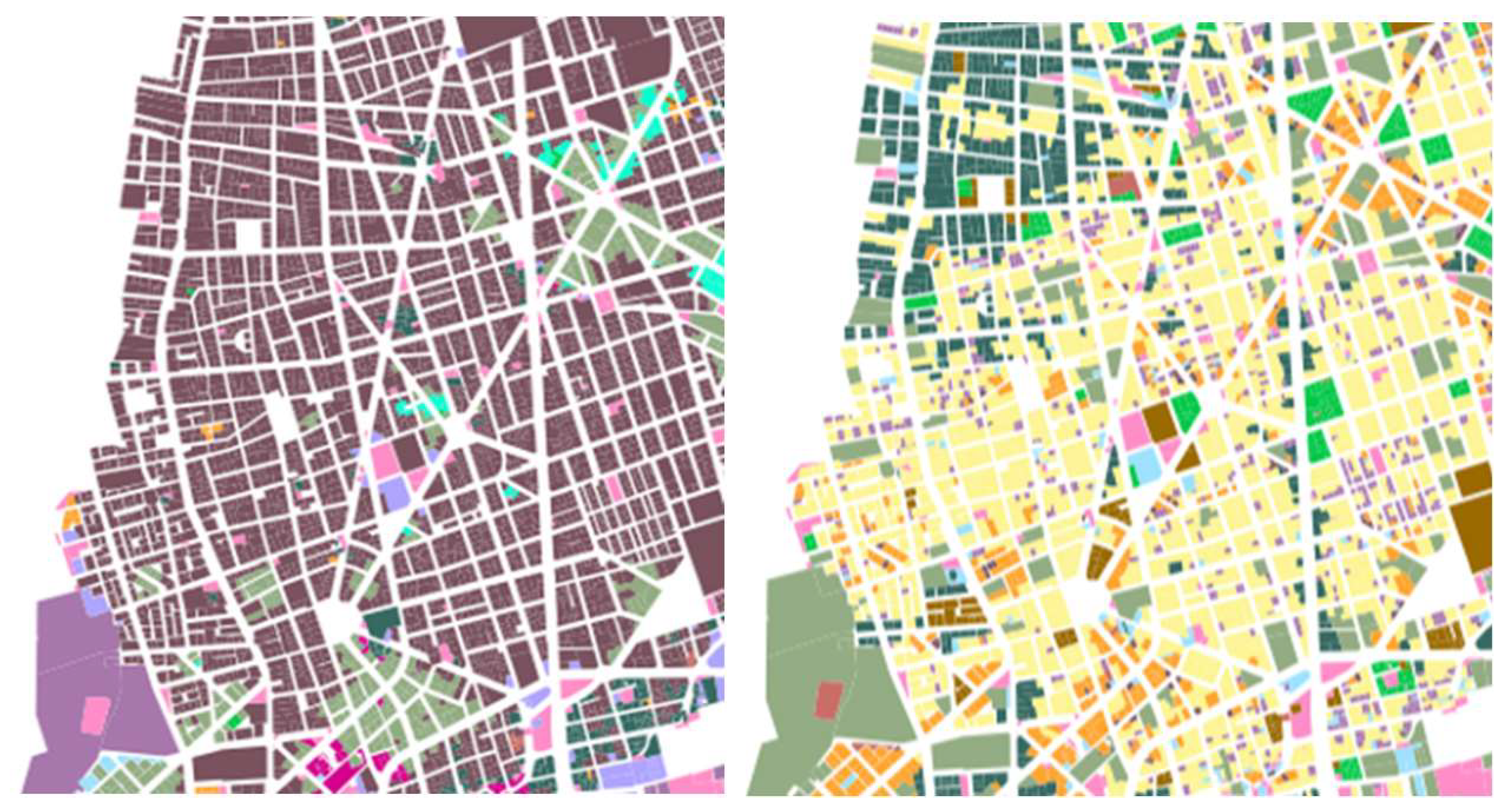
Figure 9.
Cluster profiles based on mean Gi* values.
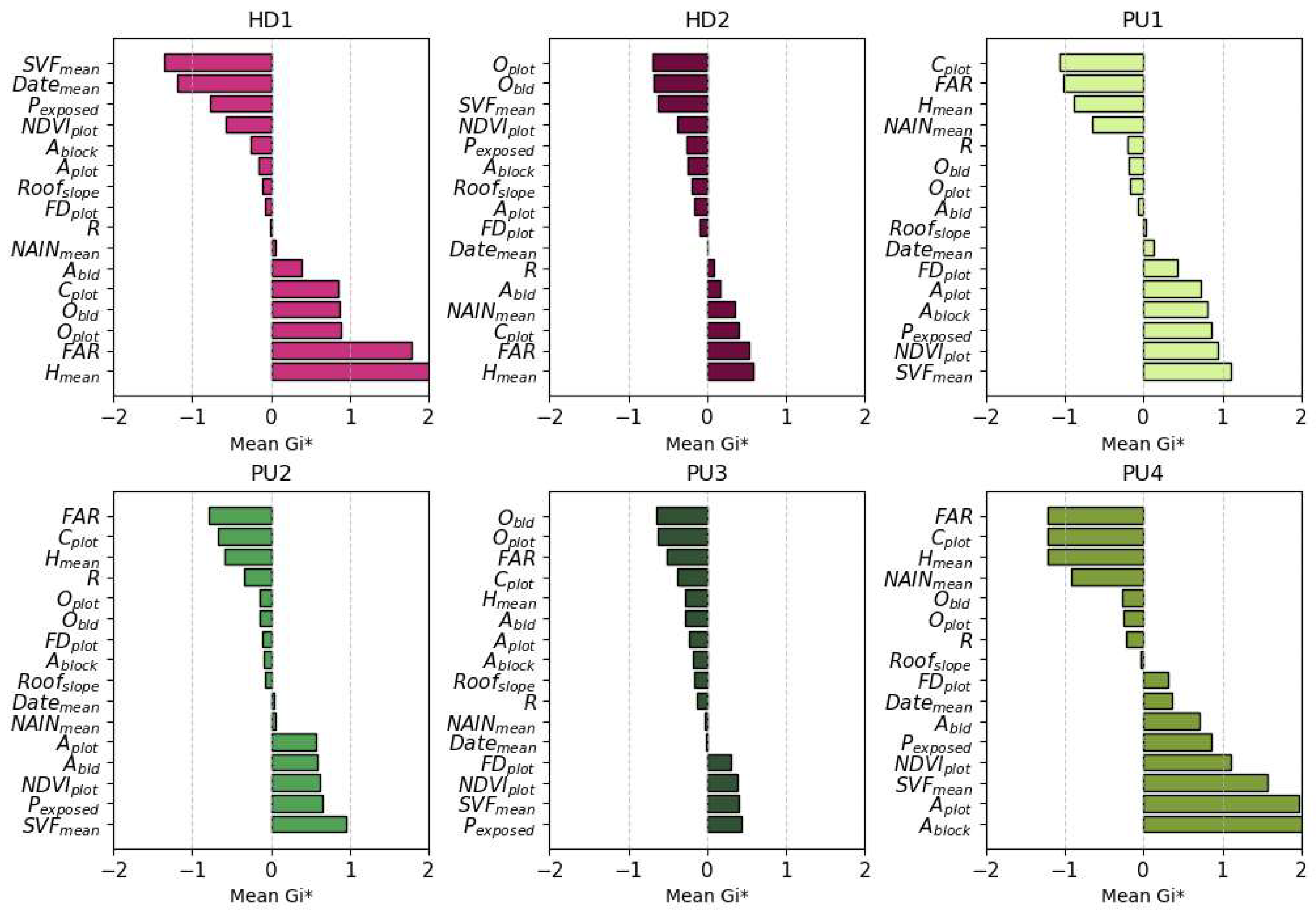
Figure 10.
Cluster profiles based on mean Gi* values (continued).
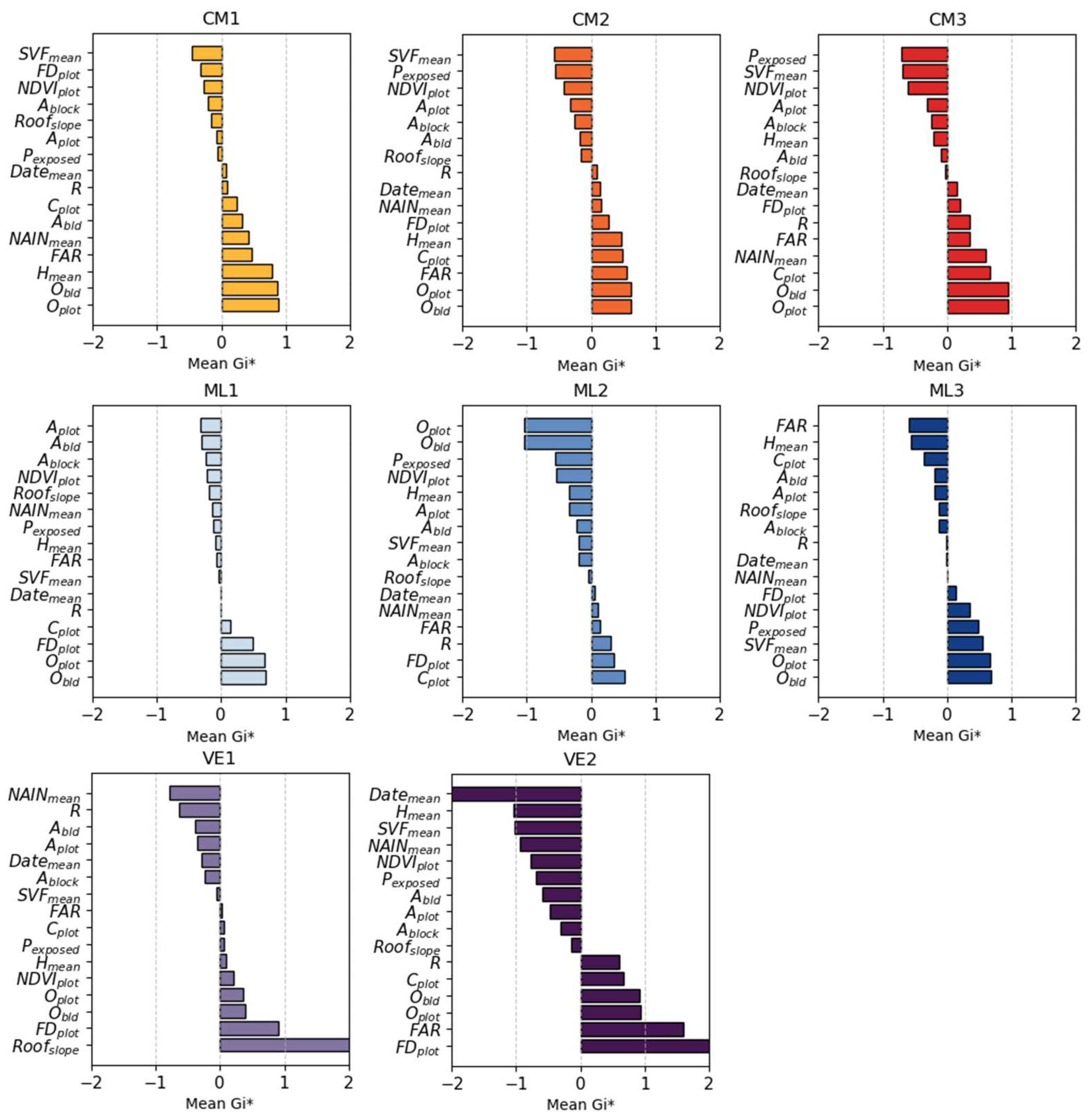
Figure 11.
Clustered urban form typologies. Basemap by Esri, DeLorme and NAVTEQ [82].
Figure 11.
Clustered urban form typologies. Basemap by Esri, DeLorme and NAVTEQ [82].
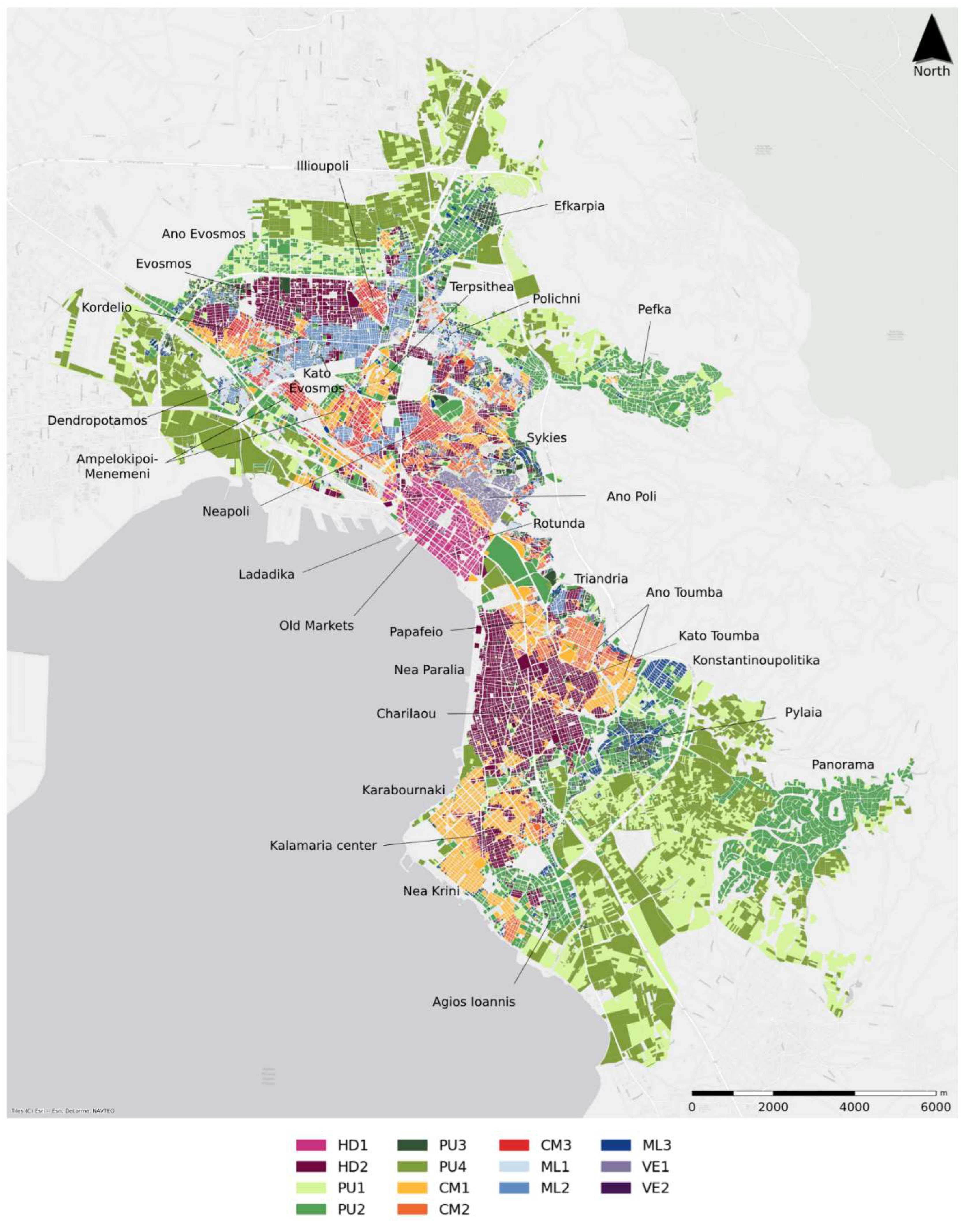
Figure 12.
Historic aerial photos of eastern (left) and western (right) neighborhoods of Thessaloniki in the first half of twentieth century [81].
Figure 12.
Historic aerial photos of eastern (left) and western (right) neighborhoods of Thessaloniki in the first half of twentieth century [81].
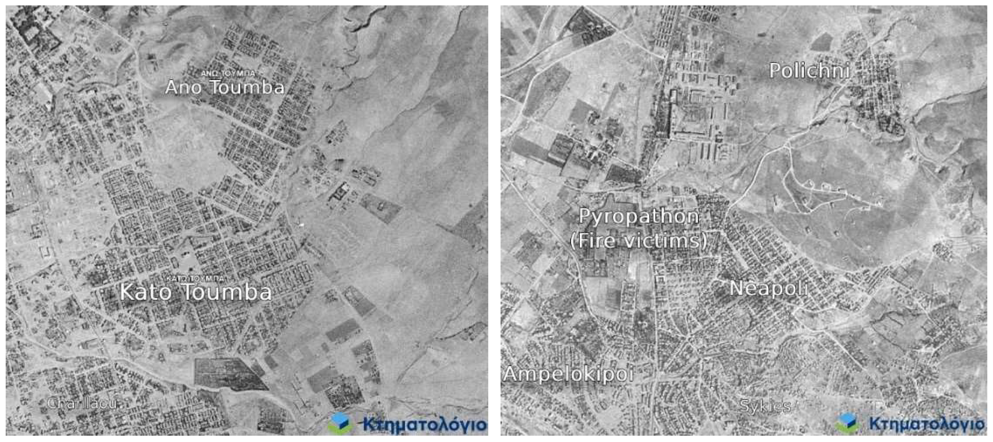
Table 4.
Data sources.
| Data | Source | Resolution/Accuracy | Comments |
| Plot geometries (89,171 plots) | Hellenic Cadastre (HC) WFS service [67] | According to HC standards, updated every 2 months. | Referenced to GGRS87 Datum. |
| Normalized Difference Vegetation Index (NDVI) | Copernicus Land Monitoring Service [68] | Derived from Sentinel-2 images at a resolution of 10m – updated daily. | Mean NDVI value calculated for 1 to 5 of June 2024, (month where peak vegetation growth coincides with little cloud cover) |
| Building footprints and street network: | OpenStreetMap [69] | Estimated at 1.6m [70] | Building footprint errors (e.g. overlapping, duplicates etc) were fixed manually. OSM street network was topologically checked, cleaned and simplified using OSMnx. |
| Building heights | Copernicus Urban Atlas (UA) [71] and Global Human Settlements Layer (GHSL) [72] | UA: 10m / ±2.9m GHSL: 30m / ±6.6m |
IDW is applied (50m max range, 12 max neighbors) to fix UA data sparsity. UA data is then superimposed on GHSL creating a composite building height raster to cover study area extents. |
| Elevation data | EU-DEM [73] | 30m / ±2.9m | Used to generate urban DSM, by adding elevation values with composite building height raster values. |
| Roof type and building date | ELSTAT 2011 census data [74] | Data aggregated at the urban block level | Aggregated data is number of buildings per time period and roof type category |
Table 5.
Global Moran’s I calculation results for the morphological indicators.
| Indicator | Moran's_I |
| 0.54 | |
| 0.33 | |
| 0.43 | |
| 0.87 | |
| NDVIplot | 0.66 |
| Cplot | 0.53 |
| 0.80 | |
| FAR | 0.65 |
| 0.97 | |
| Oplot | 0.81 |
| 0.85 | |
| NAINmean | 0.77 |
| 0.81 | |
| 0.38 | |
| 0.67 | |
| 0.71 | |
| 0.60 |
Table 6.
Hyperparameter selection for UMAP.
| Hyperparameter | Use | Value, [default] | Rationale |
| Number of components | Specifies the components (or dimensions) of the resulting latent space | 3, [2] | Min. number of clusters with meaningful variance and limited correlation |
| Neighborhood Size | defines the size of the local neighborhood used to estimate the UMAP manifold structure | 50, [15] | Consider dataset size; Favor moderately global over local structure. |
| Minimum Distance | Influences point density | 0, [0.1] | As suggested for clustering tasks [77]. |
| Metric | Determines how distances are calculated | 'canberra', [euclidean] | Encourages cluster separation. |
| Negative Sample Rate | the number of negative samples used per positive sample in gradient descent | 25, [5] | Encourages cluster separation. Scaled according to neighborhood size. |
Table 7.
Hyperparameter selection for BIRCH.
| Hyperparameter | Use | Value, [default] | Rationale |
| Threshold | Determines the maximum radius of subclusters in the CF tree. Lower values encourage splitting into many small clusters | 0.3, [0.5] | Encourage creation of smaller subclusters. |
| Branching Factor | Controls the maximum number of children nodes per non-leaf node in the CF tree. | 30, [50] | Encourage creation of smaller subclusters. |
| Number of Clusters | User-specified number of clusters for final agglomerative clustering step. | 14, [3] | Balance analytical granularity and interpretability within the study |
Table 8.
Correlation matrix of UMAP components.
| Component | Correlation with | ||
| UMAP 1 | UMAP 2 | UMAP 3 | |
| UMAP 1 | 1 | 0.16 | -0.26 |
| UMAP 2 | 0.16 | 1 | 0.00 |
| UMAP 3 | -0.26 | 0.00 | 1 |
Table 9.
Comparison of cluster quality metrics between the three scenarios.
| metric | with Gi* values and selected hyperparameters | without Gi* values and selected hyperparameters | with Gi* values and default hyperparameters |
| Silhouette Score | 0.53 | 0.42 | 0.32 |
| JS Divergence | 4.72 | 4.02 | 3.65 |
| IBR | 0.90 | 0.87 | 0.81 |
Table 10.
Urban form types.
| Family | Clusters | Characteristics | Example locations |
| High-density urban core | HD1 | Exclusively found in the historic city center. Characterized by tall buildings arranged in compact configurations, small plots with minimal vegetation on a mostly intercardinal grid. |
Historic city center |
| HD2 | Similar to HD1, with the main exceptions being a more integrated (i.e. dense and regular) and cardinally oriented grid. | Evosmos and Kordelio (west), Nea Paralia, Charilaou, Papafeio, Kalamaria center, Triandria and Kato Toumba (east) | |
| Peri-urban development |
PU1 |
Sparse configurations of low detached buildings on large plots or vacant plots, minimal urban integration, high openness and significant vegetation coverage. | City outskirts, both east and west |
| PU2 | Mostly suburban residential development on large plots with plenty of vegetation. | Panorama, Pylaia and Agios Ioannis (east), Pefka and Efkarpia (west). | |
| PU3 | Suburban cores characterized by compact arrangements of low buildings, smaller and more irregular plots than PU2 with moderate vegetation coverage. | Pylaia (east), Efkarpia (west), parts of Sykies | |
| PU4 | Newer “big box” developments on large plots, such as warehouses, exhibitions, retail parks, health and education campuses. | City outskirts both east and west. | |
| Compact midrises | CM1 |
Midrise buildings, moderately low sky openness, strong network integration, rectangular plots and intercardinal grid orientation. | Ano Toumba, Karabournaki, Nea Krini (east) and Terspithea, parts of Kordelio and Sykies (west) |
| CM2 |
Similar to CM1, characterized by more compact building arrangements and non-rectangular plot shapes. | Part of Ano Toumba (east), parts of Sykies and Neapoli (west) | |
| CM3 | Very tight arrangements of midrises with minimal vegetation. Small plot and block sizes forming a highly integrated intercardinal grid. | Exclusive to western neighborhoods (Neapoli, Ilioupoli, Ampelokipoi-Menemeni) | |
| Mixed midrises and lowrises | ML1 | Mixed building heights, small irregular plots with an intercardinal orientation and lack of vegetation. | Fringe areas between clusters, concentrated around Dentropotamos and Policnhi (west). |
| ML2 | Similar to ML1, with significantly more compact arrangements of buildings, little vegetation and a strong cardinal grid orientation. | Mostly found in Kato Evosmos and Neapoli (west) | |
| ML3 | Mix of detached lowrises and midrises with more openness and vegetation than ML1 and ML2, arranged in a compact intercardinal grid. | Mostly found in Konstantinoupolitika and Pylaia core | |
| Vernacular tissue | VE1 | Areas with predominant sloped roofs, irregular plot shapes, older buildings and low street integration. | Ano Poli and Ladadika districts |
| VE2 | Unique to the historic markets of Thessaloniki: compact configurations of very small plots, minimal vegetation, and old lowrise buildings. | Old Markets |
Disclaimer/Publisher’s Note: The statements, opinions and data contained in all publications are solely those of the individual author(s) and contributor(s) and not of MDPI and/or the editor(s). MDPI and/or the editor(s) disclaim responsibility for any injury to people or property resulting from any ideas, methods, instructions or products referred to in the content. |
© 2025 by the authors. Licensee MDPI, Basel, Switzerland. This article is an open access article distributed under the terms and conditions of the Creative Commons Attribution (CC BY) license (http://creativecommons.org/licenses/by/4.0/).
Copyright: This open access article is published under a Creative Commons CC BY 4.0 license, which permit the free download, distribution, and reuse, provided that the author and preprint are cited in any reuse.


