Mapping Ecosystem Functional Groups in the Republic of Korea Based on the IUCN Global Ecosystem Typology

Kyungil Lee; Haedam Baek; Chul Hyun Choi; Sang Hak Han; Seonyoung Park

doi:10.20944/preprints202504.1402.v1

Submitted:

16 April 2025

Posted:

16 April 2025

You are already at the latest version

Abstract

This study presents a national-scale mapping of Ecosystem Functional Groups (EFG) in the Republic of Korea using the IUCN Global Ecosystem Typology (GET), integrated with national-level spatial datasets, satellite imagery, and a Random Forest (RF) classifier. By incorporating locally relevant ecological data, the original typology was refined to resolve issues of overgeneralization and spatial overlap. The resulting map delineates 20 distinct ecosystem types, offering improved spatial accuracy and better alignment with the actual land extent. To evaluate the potential of EFG classification, the RF model was trained on seasonal satellite composites and environmental variables, achieving an overall accuracy of 80%. Elevation and temperature were found to be the most influential predictors, effectively distinguishing ecological patterns across diverse landscapes. This integrated approach supports consistent tracking of ecosystem changes and helps address the limitations of static or infrequently updated spatial datasets. The developed EFG map supports biodiversity conservation by providing a practical foundation for national spatial planning and contributing to Red List of Ecosystems assessments, in line with the goals of the Global Biodiversity Framework.

Keywords:

IUCN GET

;

biodiversity

;

ecosystem extent

;

remote sensing

;

random forest

Subject:

Environmental and Earth Sciences - Remote Sensing

1. Introduction

Biodiversity plays a critical role in maintaining ecosystem functioning and stability by promoting efficient resource utilization and strengthening resilience to environmental heterogeneity through the differential functional responses of species [1]. The adoption of the post-2020 global biodiversity framework (GBF) under the Convention on Biological Diversity [2] and the 2030 Sustainable Development Goals [3] constitutes a pivotal global policy response to address the primary drivers of biodiversity loss. In line with global trends, habitats for wildlife such as forested areas are also gradually declining in the Republic of Korea (ROK) [4]. In response, based on legal grounds and in alignment with the specific targets outlined in the GBF, ROK has developed its National Biodiversity Strategies and Action Plans (NBSAP), reflecting the national context.

Both the GBF and Korea’s NBSAP emphasize spatial planning as a foundational strategy for identifying ecologically significant areas and setting conservation priorities. Monitoring the spatial extent and configuration of ecosystem types is essential to support this approach, requiring robust indicators and methodologies that capture ecosystem structure, function, and composition [5]. Moreover, this objective also supports ecosystem condition assessments and conservation prioritization, particularly through the application of the International Union for Conservation of Nature (IUCN) Red List of Ecosystems (RLE), which provides a global standard for evaluating the risk of ecosystem collapse based on indicators such as area change, range contraction, environmental degradation, and biotic disruption [6,7].

To implement such monitoring frameworks at a global scale, the use of standardized ecosystem typologies and spatial units is essential. In this context, Remote Sensing (RS) data such as multispectral and radar imagery from satellites are increasingly utilized due to their accessibility and broad spatial coverage [8,9,10,11]. Recent studies have actively applied RS data in combination with artificial intelligence (AI) based classifiers, particularly machine learning techniques, to enhance the monitoring of ecosystem related indicators [12,13,14,15,16]. However, existing ecosystem monitoring studies have shown considerable variation in data sources, typological frameworks, and methodological approaches. This heterogeneity impedes the comparability of monitoring results across regions and the consistent tracking of global ecosystem trends. In addition, commonly used land cover classifications often provide limited representation of ecosystem functions and biotic components, constraining comprehensive assessments of ecosystem condition [17].

To establish standardized and spatially explicit ecosystem categories and terminology applicable at the global scale, the IUCN developed the Global Ecosystem Typology (GET), which incorporates ecosystem functions and processes [18]. The GET is structured into a six-level hierarchical framework. The upper three levels include: Level 1 (Realm), comprising 10 major and transitional ecosystem realms; Level 2 (Biome), which further classifies realms into 25 biomes; and Level 3 (Ecosystem Functional Group, EFG), which divides biomes into 110 functionally distinct ecosystem groups. Levels 4 through 6 are designed to capture compositional variations within functionally convergent ecosystem groups, enabling finer-scale classification at national and subnational levels [18]. Although the GET has been recommended as a standardized framework for ecosystem classification and as the assessment unit for the IUCN RLE [19], its application remains challenging. This is primarily due to insufficient spatially detailed data at national scales, and classification uncertainties including excessive overlap among ecosystem types. Moreover, studies on mapping ecosystem types based on the IUCN GET remain limited, and evaluations of the applicability of RS data and AI techniques for this purpose are also insufficient.

In this study, a national-scale map of EFGs based on the GET framework was developed for the Republic of Korea, utilizing environmental thematic maps and geospatial datasets to enable international comparability. In addition, given that national-scale maps based on pre-existing spatial data may not fully reflect current ecosystem conditions, the mapping approach was further evaluated using satellite imagery and a Random Forest (RF) algorithm.

2. Materials and Methods

2.1. Study Area

The study area is located between approximately 33°N–39°N latitude and 124°E–132°E longitude, covering an area of approximately 100,000 km² (Figure 1). The region has a warm monsoon climate with hot summers (June to August) and cold, dry winters (December to February), resulting in pronounced seasonal variation in phenology and ecological dynamics [20]. Examples from the original IUCN GET maps reveal limitations when applied at the national scale (https://global-ecosystems.org/analyse, accessed on 10 September 2024) (Figure 1c1-1c4)). Types such as T7.3 and T7.4 cover almost the entire country, suggesting overgeneralization, while F3.1 and MT1.2 present spatial mismatches, both cases demonstrate inaccuracies due to coarse resolution and generalized input layers. These observations underscore the challenges in directly utilizing the original GET maps for ecosystem assessments within this region.

2.2. Data Acquisition and EFG map Development

Firstly, to develop the EFG map for ROK, we identified the ecosystem types currently present in the country based on the IUCN GET. Considering the available spatial data as of 2022 and expert consultations, we selected 20 types applicable to the national context and established a classification framework for each. Table A1 in Appendix A lists the source data used for the classification and mapping [21,22,23,24,25,26,27,28,]. Table A2 in Appendix A shows the classification criteria for each EFG. All source data were projected to the UTM/WGS84 coordinate system and resampled to 30 m spatial resolution for alignment with satellite imagery. The spatial classification of each EFG was derived using land cover-related datasets provided by the respective government agencies. Functional classification was applied on top of spatial classification to produce the EFG map, integrating environmental and land cover variables. This process was based on the key drivers of each EFG proposed by [18] and refined through expert consultation to reflect national conditions in the ROK.

Seasonal composites of Landsat 8–9 Level-2 satellite imagery for the year 2022 were generated using Google Earth Engine (GEE) as input data for EFG classification modeling based on the constructed EFG map. GEE is a cloud-based geospatial analysis platform that allows efficient processing of large-scale satellite datasets without the need for local storage or high-performance computing [29]. During the compositing process, cloud masking was also applied to ensure high-quality observations. The seasons were defined as winter (12–2), spring (3–5), summer (6–8), and autumn (9–11). Table 1 summarizes the input variables used in the classification model, including spectral indices and a thermal band derived from the constructed Landsat composite imagery [30,31].

2.3. Random Forest Modeling

We employed the RF algorithm to construct the EFG classification model because of its strong performance in ecological classification tasks. The RF algorithm has been widely applied in remote sensing tasks involving both classification and regression [32]. It consists of an ensemble of Classification and Regression Trees (CARTs), each trained on a randomly selected subset of the input data [33]. For every CART, predictor variables are selected at random with equal probability. The final prediction is obtained by aggregating the outputs of all individual trees, either through majority voting (for classification) or averaging (for regression). This ensemble strategy, which integrates bootstrap aggregation (bagging) and random feature selection, has been demonstrated to outperform many other machine learning approaches in various contexts [34].

The input datasets for modeling consisted of 25 bands, including seasonal variables derived from Landsat as presented in Table 1, seasonal mean temperatures based on 5-year MK-PRISM data, and DEM (Table A1). Considering the spatial extent of each EFG and to ensure a balance between model performance and computational efficiency, we extracted 500 to 1,000 samples per class using stratified random sampling. This range has been shown to be sufficient for robust classification, particularly when using ensemble models such as RF [35]. We trained the models using a random selection of 80% of samples, stratified by EFG class, and the remaining 20% was used for test.

RF model was tuned using training dataset and grid search with 5-fold cross-validation while systematically refining key parameters such as n_estimators, max_depth, min_samples_split, and min_samples_leaf. After parameter optimization, we assessed the model performance using the test dataset and the metrics presented in Table 2. TP, FP, and FN refer to true positives, false positives, and false negatives for the target class, respectively; T and F denote the total number of correctly and incorrectly classified points across all classes. RF modeling was performed using scikit-learn python 3.8.10 library.

3. Results

3.1. Result of EFG map Development for the Republic of Korea

We classified a total of 20 EFG types within the ROK based on various data suitable for ecosystem classification, expert opinions, and the definitions provided in the existing IUCN GET. Figure 4(left) shows the developed EFG map, and Table 3 presents the area of each EFG type in both the EFG map and the existing IUCN GET. Compared to the original IUCN GET classification, the EFG map developed in this study includes several structural refinements and additions. For example, T2.2 (Temperate Forests) has been subdivided into more specific categories: T2.2.1 (Broadleaved Temperate Forests), T2.2.2 (Coniferous Temperate Forests), and T2.2.3 (Mixed Temperate Forests). In addition, new functional groups that were not present in the original GET, such as TF1.3 (Permanent Marshes), TF1.7 (Boreal and Temperate Fens), and F1.2 (Permanent Lowland Rivers), have been introduced, improving ecological specificity.

Significant differences were observed in the spatial extent of many EFG types in the refined map (Table 3). T2.1 (Montane Forests) showed a drastic decrease of over 99%, which may be due to climatic thresholds from [18], as many areas did not meet the required number of months with mean temperatures above 10°C. T2.2.1 decreased compared to the undivided T2.2 in the original GET, but the combined area of T2.2.1 to T2.2.3 (59,796.32 km²) exceeded the original value, suggesting internal redistribution and improved vegetation classification. T2.4 (Warm Temperate Laurophyll Forests) also showed a substantial reduction of about 99%, likely due to refined interpretation of vegetation types.

Among agricultural and artificial ecosystems, some types were broadly overestimated in the original GET due to generalized classification and coarse spatial resolution over 1 km. Among them, F3.3 (Rice Paddies), T7.2 (Horticultural Croplands), T7.3 (Plantations), and T7.4 (Urban and Industrial Ecosystems) were mapped across nearly the entire national territory, resulting in very low spatial accuracy. These types have been significantly refined in the developed EFG map through more detailed classification and spatial filtering. As a result, T7.3 decreased by 98%, F3.3 by 78%, and T7.1 (Annual Croplands) by 63%. Similarly, T7.5 (Derived Semi-natural Pastures and Old Fields) declined by 87%, and T7.4 by 84%, reflecting a comprehensive correction of prior overestimation across managed landscapes.

Wetland and river-related types also showed substantial changes. TF1.2 (Subtropical–Temperate Forested Wetlands) decreased by over 99.99%, while TF1.3 and TF1.7, which were not included in the original GET, were newly added. F1.1 (Permanent Upland Streams), F1.3 (Freeze-thaw Rivers), F1.4 (Seasonal Upland Streams), and F1.5 (Seasonal Lowland Rivers) were reduced by over 95–98%, while F1.2 was newly mapped, reflecting improved hydrological delineation. F2 (Lakes) increased by 93% due to more accurate detection of inland water bodies and MT1 (Shorelines) declined by 68%, likely due to refined coastal boundary definitions and the removal of spatial overlaps.

The total area assigned to the 20 EFG types in the original IUCN GET was 414,258 km², approximately four times the actual land area of South Korea (about 100,000 km²), primarily due to broadly defined and overlapping classifications. In contrast, the refined EFG map developed in this study maps a total of 105,684.97 km² including MT1, closely matching the actual land area. This demonstrates a significant improvement in spatial accuracy and consistency over the original GET.

Table 3. Area comparison between IUCN GET and the developed EFG map for each EFG type.

ID	Ecosystem Functional Group	EFG map (km²)	IUCN GET (km²)
T2.1	Boreal and temperate montane forests and woodlands	19.48	3195.06
T2.2.1	Broadleaved Temperate Forests	32076.05	46114.35
T2.2.2	Coniferous Temperate Forests	20964.80
T2.2.3	Mixed Temperate Forests	6755.47
T2.4	Warm temperate laurophyll forests	142.68	13838.58
T7.1	Annual croplands	11235.81	30683.18
T7.3	Plantations	1268.27	79767.46
T7.4	Urban and industrial ecosystems	9918.62	61680.09
T7.5	Derived semi-natural pastures and old fields	4666.41	36347.7
TF1.2	Subtropical-temperate forested wetlands	3.12	42663.56
TF1.3	Permanent marshes	24.23	NA
TF1.7	Boreal and temperate fens	1.45	NA
F1.1	Permanent upland streams	172.41	7279.39
F1.2	Permanent lowland rivers	210.50	NA
F1.3	Freeze-thaw rivers and streams	290.53	11998.11
F1.4	Seasonal upland streams	171.72	18313.1
F1.5	Seasonal lowland rivers	31.11	2178.58
F2	Lakes	3387.31	1753.99
F3.3	Rice paddies	9974.73	44601.29
MT1	Shorelines	4370.31	13843.88
Total		414258.32	105684.97

3.2. Classification Results

Developed EFG map was used as the reference map to perform EFG classification using satellite imagery and RF algorithm. Accuracy assessments for each EFG type are presented in Table 4, and the confusion matrix for the classification results is shown in Figure 2.

The model achieved an overall accuracy of 0.80, with particularly high performance observed in classes such as T2.1, T2.4, F1.1, F1.2, F2, and MT1, all of which recorded F1-scores above 0.90. In contrast, TF1.3, TF1.7, and F1.3 yielded F1-scores below 0.50, largely due to confusion with ecologically similar or spatially adjacent categories. For example, TF1.3 samples were frequently misclassified as TF1.7 and T2.2.3 (mixed temperate forests), reflecting the difficulty of distinguishing wetland ecosystems with variable vegetation structure. F1.3, which is defined by seasonal freezing conditions and winter temperatures below 0°C, also showed more frequent misclassification compared to other riverine classes such as F1.1 and F1.2. This suggests challenges in capturing the spectral or seasonal variability of intermittent or thermally dynamic water bodies. T7.4 also exhibited notable misclassifications, particularly with T2.2.3, T7.1, and T7.5. These overlaps are likely due to the complex spatial heterogeneity in peri-urban areas, where built-up surfaces, cropland edges, and vegetated open spaces are often intermingled, making them difficult to distinguish based on spectral features alone. Additionally, T2.2.3 was also confused with T2.2.1 and T2.2.2, highlighting the challenges of delineating transitional forest types that share similar structural and climatic characteristics.

Table 4. Accuracies of the RF model for EFG classification.

Division	Precision	Recall	F1-score
T2.1	0.98	0.95	0.96
T2.2.1	0.76	0.91	0.83
T2.2.2	0.74	0.89	0.80
T2.2.3	0.81	0.89	0.84
T2.4	0.98	0.87	0.92
T7.1	0.7	0.9	0.79
T7.3	0.83	0.8	0.82
T7.4	0.53	0.84	0.65
T7.5	0.73	0.59	0.65
TF1.2	1.00	0.67	0.8
TF1.3	1.00	0.45	0.62
TF1.7	0.91	0.32	0.47
F1.1	0.99	0.95	0.97
F1.2	0.92	0.92	0.92
F1.3	0.79	0.15	0.25
F1.4	0.78	0.63	0.70
F1.5	0.89	0.74	0.81
F2	0.93	0.97	0.95
F3.3	0.75	0.97	0.85
MT1	0.96	0.97	0.97
Overall accuracy	0.80

Figure 2. Confusion matrix for EFG classification using RF.

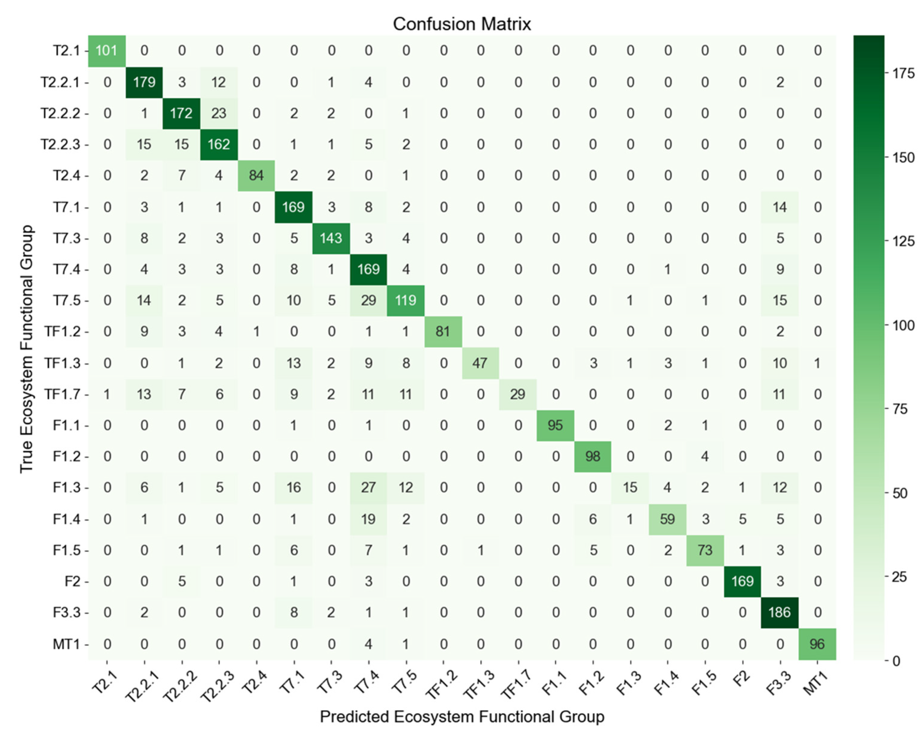
Figure 3 shows the feature importance of the 25 predictors used in RF classification for EFGs. DEM was the most important variable, effectively separating elevation-dependent classes such as montane forests and highland wetlands. Temperature-related variables, including seasonal averages from MK-PRISM and Landsat LST, also showed strong influence. These variables played a key role in distinguishing ecosystems characterized by climatic conditions and seasonal variability, with predictors from multiple seasons contributing meaningfully to the classification. Spectral variables based on surface reflectance, which are commonly used in land cover classification for their sensitivity to vegetation greenness, surface moisture, and built-up features [36], showed moderate importance in the model. These variables contributed consistently across seasons, aiding the classification of EFG types without notable seasonal variation in their relative importance.

3.3. Mapping Results

Figure 4(right) shows the EFG mapping result for the entire ROK using the RF model. While the overall distribution is similar to the reference EFG map (left), T7.4 (urban and industrial ecosystems) is more broadly mapped, particularly in peri-urban areas where it tends to be confused with T2.2.3, T7.1, and T7.5, as previously described. Additionally, T2.1 (boreal and temperate montane forests) is more extensively mapped in mountainous regions, likely due to the influence of DEM. In contrast, the reference map reflects more conservative delineation based on temperature criteria, leading to visible differences in high altitude areas. Shorelines are also generally well reproduced in the RF classification, although certain areas in the northwestern coastal region were classified as F2, possibly due to spectral similarity near land water boundaries.

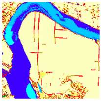
Table 5 demonstrates that the EFG map constructed using nationally developed environmental thematic maps, can differ from the results of RF modeling based on satellite imagery. In Case 1, such discrepancies appear in areas containing sensitive infrastructure, such as military facilities, where access to accurate ground information may be restricted due to security concerns [37]. In Case 2, environmental maps developed at the national level, which are updated less frequently than satellite imagery, often fail to capture recent changes in land surface conditions. These cases highlight the limitations of relying solely on pre-existing spatial data for monitoring EFG dynamics, and emphasize the need to incorporate satellite imagery and AI-based modeling approaches as complementary tools to improve the accuracy and timeliness of ecosystem monitoring.

Figure 4. EFG map of the Republic of Korea developed in this study and classification result based on satellite imagery and random forest classifier.

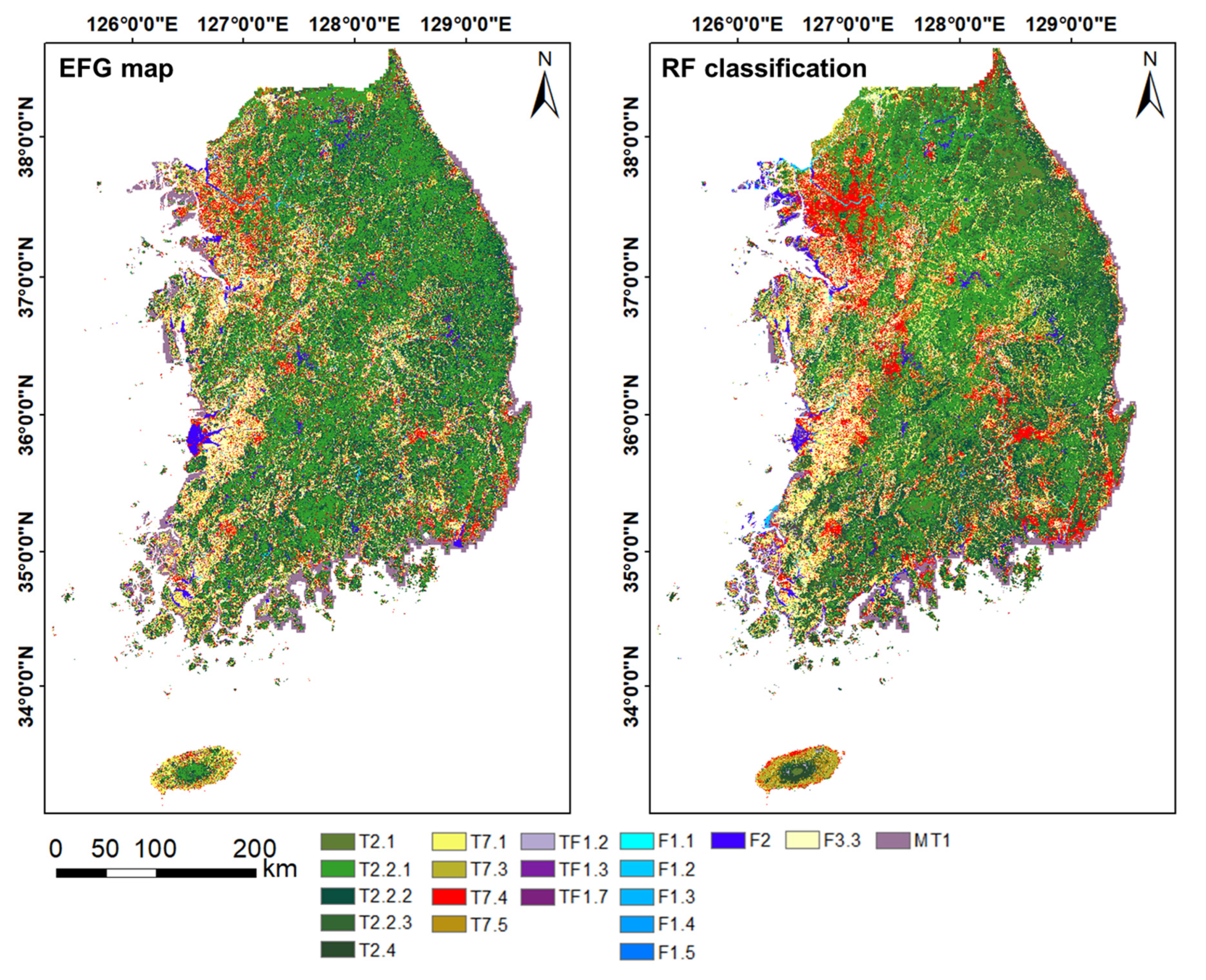
Table 5. Case-specific differences between EFG map and RF modeling results.

	True color	EFG map	RF mapping
Case A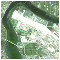
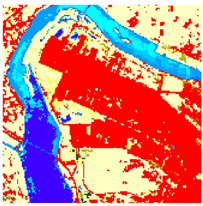Case B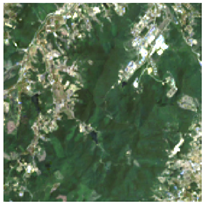

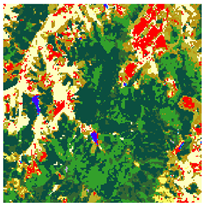4. Discussion

A globally standardized ecosystem classification provides the foundation for consistent assessment, monitoring, and conservation planning, regardless of regional or national boundaries. By offering a unified typological framework, it enables the integration of heterogeneous ecological data and facilitates meaningful global comparisons. In particular, such a framework is essential for applications such as the IUCN RLE, which relies on uniform criteria to assess ecosystem risk and guide prioritization [19]. This study applied the IUCN GET framework to ROK as a test case and demonstrated how national-level spatial datasets can be integrated with remote sensing data to derive a higher resolution EFG map. Compared to the original GET map, which often overgeneralizes or misrepresents local ecological patterns, our results underscore the value of incorporating contextualized ecological information. Notably, substantial differences were observed in the distribution and area of specific EFG types, demonstrating the enhanced ability of our approach to capture local ecological variation. By incorporating ecological data from national sources, the method improves classification accuracy and mitigates the limitations of globally generalized ecosystem maps [38]. In addition, this refinement supports more accurate representation of ecosystem heterogeneity, which is critical for monitoring of ecosystems and supporting conservation and policy decisions [39].

To evaluate the feasibility of satellite-based classification of EFGs, we employed an RF algorithm trained on diverse geospatial predictors. Among these, DEM was the most influential, reflecting the significant relationship between topography and ecological variation. Elevation influences spatial patterns in vegetation and ecosystem composition by shaping hydrological processes, microclimates, and soil conditions, all of which affect the distribution of EFGs [40,41]. Temperature-related variables, the integration of MK-PRISM and Landsat-derived LST, showed high feature importance, indicating their potential relevance in differentiating EFGs based on thermal characteristics. As demonstrated by [42], canopy and temperature dynamics are associated with ecological function and species traits, particularly in forests and wetlands. Although spectral indices contributed valuable spatial information, their importance was somewhat lower than that of topographic and thermal variables. Nevertheless, as suggested by [41], they were crucial for distinguishing EFGs in complex environments, such as urban-natural ecotones or ecosystems with seasonal phenological changes. Overall, the integration of topographic, thermal, and spectral data within a RF algorithm demonstrates the potential of satellite-based approaches for functionally meaningful ecosystem classification. Additionally, timely ecosystem monitoring is essential for informing effective policy decisions, as emphasized by [38]. This study demonstrates that such needs can be addressed and complemented through the integration of satellite-derived mapping results with the constructed EFG map, enabling more spatiotemporally representative monitoring.

The significance of this study lies in presenting an integrated methodology that synthesizes detailed national-level spatial datasets, satellite-based geospatial variables, and AI-based classification techniques to produce EFG map aligned with the IUCN GET framework. This approach demonstrates the practical feasibility of applying globally standardized ecosystem typologies within a regional context while enhancing the spatial resolution and ecological specificity of classification outputs. However, due to limitations in data and definitions, specific EFG types were not included in the current classification, highlighting the importance of integrating overlooked EFG types to improve ecological accuracy and representational completeness. Building on this foundation, subsequent efforts should focus on including a broader range of EFG types, integrating more diverse datasets, and applying advanced deep learning-based models to support more ecologically meaningful and spatially accurate EFG mapping.

5. Conclusions

This study applied the IUCN GET to map EFGs in ROK by integrating national-level spatial datasets, satellite imagery, and an RF classifier. First, based on national-level spatial datasets, an optimized EFG map for ROK was developed that more accurately captures local ecological heterogeneity and better aligns with the actual land extent than the original GET product. This refinement addressed issues such as overgeneralization and spatial overlap commonly found in globally generalized typologies. Subsequently, satellite imagery and geospatial variables were incorporated using an RF classifier to assess the applicability of automated classification. Variables related to elevation and temperature had the greatest influence on the model, underscoring their critical role in distinguishing EFGs across diverse ecological gradients. The mapping result offers complementary value for ecosystem monitoring by supporting consistent detection of spatial changes and offering insight into region specific ecological patterns. It also helps to address the limited update frequency of existing national-level spatial datasets, underscoring the value of satellite-based automated mapping for more timely and responsive ecosystem assessments. These improvements provide a stronger basis for ecosystem monitoring and more coherent conservation decision-making by enabling standardized and spatially consistent assessments. The optimized EFG map for ROK, built from national-level datasets and remote sensing, serves as a practical tool for domestic planning while enhancing compatibility with global frameworks. In particular, it offers a robust input for IUCN RLE assessments, contributing to consistent evaluation of ecosystem risks and supporting global biodiversity conservation efforts in alignment with the goals of the GBF.

Author Contributions

Designed the methodology, K.L. and S.P.; provided and validated data, C.H.C. and S.H.H.; performed the data processing, K.L., H.B. and S.P.; formal analysis, K.L. and H.B.; writing-original draft preparation, K.L.; writing-review and editing, S.P. All authors have read and agreed to the published version of the manuscript.

Funding

This research was supported by the National Institute of Ecology with funding from the Ministry of Environment of the Republic of Korea (NIE-B-2025-43) and the National Research Foundation of Korea (NRF) grant funded by the Korea Ministry of Science and ICT (MSIT) (2022R1C1C1013225).

Conflicts of Interest

The authors declare no conflicts of interest.

Appendix A

Table A1. Datasets used for the development of the EFG map for Republic of Korea.

Application	Dataset	Description	Creator	Extent	Time	Sources	Reference
Spatial classification	Land cover map	Nationwide land cover data classified into 41 classes	ME	ROK	2022	https://egis.me.go.kr	[21]
	Forest type map	Spatial distribution of forests by type, origin, and other attributes	KFS	ROK	2022	https://map.forest.go.kr	[22]
	Farm map	Spatial distribution of farmlands by type	MAFRA	ROK	2022	https://agis.epis.or.kr	[23]
	Wetland inventory	Spatial distribution of wetlands by type	NIE	ROK	2022	https://www.data.go.kr/en/index.do	[24]
Functional classification	JRC global surface water	Information on surface water occurrence and seasonality	JRC	Global	2021	https://global-surface-water.appspot.com/	[25]
	HydroRIVERS	Information on river geometry and order	WWF	Global	2020	https://www.hydrosheds.org/	[26]
	MK-PRISM	Nationwide gridded mean air temperature	KMA	ROK	2015-2019	http://www.climate.go.kr/	[27]
	DEM	Nationwide gridded surface elevation	NGII	ROK	2022	https://map.ngii.go.kr/	[28]
Notes: ROK, Republic of Korea; ME, Ministry of Environment of the Republic of Korea; KFS, Korea Forest Services; MAFRA, Ministry of Agriculture, Food and Rural Affairs of the Republic of Korea; NIE, National Institute of Ecology of the Republic of Korea; JRC, Joint Research Centre of the European Commission; WWF, World Wildlife Fund; KMA, Korea Meteorological Administration; NGII, National Geographic Information Institute

Table A2. Classification framework for each EFG.

ID	Ecosystem Functional Group	Criteria
T2.1	Boreal and temperate montane forests and woodlands	Vegetation areas based on land cover map 1–3 months averaging above 10°C based on 5-year MK-PRISM data Elevation above 1,000 m based on DEM
T2.2.1	Broadleaved Temperate Forests	Broadleaved forests based on forest type map Winter mean temperature below 1°C, summer mean temperature at or below 22°C, and 4–6 months averaging above 10°C based on 5-year MK-PRISM data Elevation below 1,000 m based on DEM
T2.2.2	Coniferous Temperate Forests	Coniferous forests based on forest type map Winter mean temperature below 1°C, summer mean temperature at or below 22°C, and 4–6 months averaging above 10°C based on 5-year MK-PRISM data Elevation below 1,000 m based on DEM
T2.2.3	Mixed Temperate Forests	Mixed forests based on forest type map Winter mean temperature below 1°C, summer mean temperature at or below 22°C, and 4–6 months averaging above 10°C based on 5-year MK-PRISM data Elevation below 1,000 m based on DEM
T2.4	Warm temperate laurophyll forests	Evergreen broadleaved forest based on forest type map 6–8 months averaging above 10°C based on 5-year MK-PRISM data Elevation below 1,000 m based on DEM
T7.1	Annual croplands	Fields based on farm map
T7.3	Plantations	Orchards based on farm map
T7.4	Urban and industrial ecosystems	Built-up areas and artificial bare areas based on land cover map
T7.5	Derived semi-natural pastures and old fields	Natural and artificial grassland based on land cover map
TF1.2	Subtropical-temperate forested wetlands	Inland wetlands based on land cover map Woody vegetation area based on wetland inventory
TF1.3	Permanent marshes	Lakes, rivers, and wetlands smaller than 8 hectares based on wetland inventory
TF1.7	Boreal and temperate fens	Inland wetlands based on land cover map Herbaceous vegetation area based on wetland inventory
F1.1	Permanent upland streams	Rivers based on land cover map 1st to 3rd order rivers based on HydroRIVERS Permanent water based on JRC global surface water
F1.2	Permanent lowland rivers	Rivers based on land cover map 4th to 9th order rivers based on HydroRIVERS Permanent water based on JRC global surface water
F1.3	Freeze-thaw rivers and streams	Rivers based on land cover map Winter mean temperature below 0°C based on 5-year MK-PRISM data
F1.4	Seasonal upland streams	Rivers based on land cover map 1st to 4th order rivers based on HydroRIVERS Seasonal water based on JRC global surface water
F1.5	Seasonal lowland rivers	Rivers based on land cover map 5th to 9th order rivers based on HydroRIVERS Seasonal water based on JRC global surface water
F2	Lakes	Lakes based on land cover map
F3.3	Rice paddies	Rice paddies based on farm map
MT1	Shorelines	Areas between marine waters based on the land cover map and inland boundaries

References

Matias, M. G.; Combe, M.; Barbera, C.; Mouquet, N. Ecological strategies shape the insurance potential of biodiversity. Front. Microbiol. 2013, 3, 432. [CrossRef] [PubMed]
Parks, L.; Tsioumani, E. Transforming biodiversity governance? Indigenous peoples' contributions to the Convention on Biological Diversity. Biol. Conserv. 2023, 280, 109933-1. [CrossRef]
Hák, T.; Janoušková, S.; Moldan, B. Sustainable Development Goals: A need for relevant indicators. Ecol. Indic. 2016, 60, 565-573. [CrossRef]
Yao, Y.; Zhang, D.; Nan, Y.; Jin, S.; Sun, Y. Environmental degradation in the Korean Peninsula: Evidence from the environmental degradation index. Ecol. Indic. 2024, 158, 111503. [CrossRef]
Hansen, A. J.; Noble, B. P.; Veneros, J.; East, A.; Goetz, S. J.; Supples, C.; Watson, J.E.M.; Jantz, P. A.; Pillay, R.; Jetz, W.; Ferrier, S.; Grantham, H.S.; Evans, T. D.; Ervin, J.; Venter, O.; Virnig, A. L. Toward monitoring forest ecosystem integrity within the post-2020 Global Biodiversity Framework. Conserv. Lett. 2021, 14(4), e12822. [CrossRef]
Bland, L. M.; Nicholson, E.; Miller, R. M.; Andrade, A.; Carré, A.; Etter, A.; Ferrer-Paris, J. R.; Herrera, B.; Kontula, T.; Lindgaard, A.; Pliscoff, P.; Skowno, A.; Valderrábano, M.; Zager, I.; Keith, D. A. Impacts of the IUCN Red List of Ecosystems on conservation policy and practice. Conserv. Lett. 2019, 12(5), e12666. [CrossRef]
Rodríguez, J. P.; Keith, D. A.; Rodríguez-Clark, K. M.; Murray, N. J.; Nicholson, E.; Regan, T. J.; Miller, R. M.; Barrow, E. G.; Bland, L. M.; Boe, K.; Brooks, T. M.; Oliveira-Miranda, M. A.; Spalding, M.; Wit, P. A practical guide to the application of the IUCN Red List of Ecosystems criteria. Philos. Trans. R. Soc. B Biol. Sci. 2015, 370(1662), 20140003. [CrossRef]
Andreatta, D.; Gianelle, D.; Scotton, M.; Dalponte, M. Estimating grassland vegetation cover with remote sensing: A comparison between Landsat-8, Sentinel-2 and PlanetScope imagery. Ecol. Indic. 2022, 141, 109102. [CrossRef]
Capotorti, G.; Del Vico, E.; Copiz, R.; Facioni, L.; Zavattero, L.; Bonacquisti, S.; Paolanti, M.; Blasi, C. Ecosystems of Italy. Updated mapping and typology for the implementation of national and international biodiversity-related policies. Plant Biosyst. 2023, 157(6), 1248-1258.
García-Pardo, K. A.; Moreno-Rangel, D.; Domínguez-Amarillo, S.; García-Chávez, J. R. Remote sensing for the assessment of ecosystem services provided by urban vegetation: A review of the methods applied. Urban For. Urban Green. 2022, 74, 127636. [CrossRef]
Murray, N. J.; Keith, D. A.; Bland, L. M.; Ferrari, R.; Lyons, M. B.; Lucas, R.; Pettorelli, N.; Nicholson, E. The role of satellite remote sensing in structured ecosystem risk assessments. Sci. Total Environ. 2018, 619, 249-257. [CrossRef]
Grabska, E.; Frantz, D.; Ostapowicz, K. Evaluation of machine learning algorithms for forest stand species mapping using Sentinel-2 imagery and environmental data in the Polish Carpathians. Remote Sens. Environ. 2020, 251, 112103. [CrossRef]
Hemmerling, J.; Pflugmacher, D.; Hostert, P. Mapping temperate forest tree species using dense Sentinel-2 time series. Remote Sens. Environ. 2021, 267, 112743. [CrossRef]
James, K.; Bradshaw, K. Detecting plant species in the field with deep learning and drone technology. Methods Ecol. Evol. 2020, 11(11), 1509-1519. [CrossRef]
Melichar, M.; Didan, K.; Barreto-Muñoz, A.; Duberstein, J. N.; Jiménez Hernández, E.; Crimmins, T.; Li, H.; Traphagen, M.; Thomas, K. A.; Nagler, P. L. Random forest classification of multitemporal Landsat 8 spectral data and phenology metrics for land cover mapping in the Sonoran and Mojave deserts. Remote Sens. 2023, 15(5), 1266. [CrossRef]
Pizarro, S. E.; Pricope, N. G.; Vargas-Machuca, D.; Huanca, O.; Ñaupari, J. Mapping land cover types for highland Andean ecosystems in Peru using google earth engine. Remote Sens. 2022, 14(7), 1562. [CrossRef]
Keith, D. A.; Ferrer-Paris, J. R.; Nicholson, E.; Bishop, M. J.; Polidoro, B. A.; Ramirez-Llodra, E.; Tozer, M. G.; Nel, J. L.; Mac Nally, R.; Gregr, E. J.; Watermeyer, K. E.; Essl, F.; Faber-Langendoen, D.; Franklin, J.; Lehmann, C. E. R.; Etter, A.; Roux, D. J.; Stark, J. S.; Rowland, J. A.; Brummitt, N. A.; Fernandez-Arcaya, U. C.; Suthers, I. M.; Wiser, S. K.; Donohue, I.; Jackson, L. J.; Pennington, R. T.; Iliffe, T. M.; Gerovasileiou, V.; Giller, P.; Robson, B. J.; Pettorelli, N.; Andrade, A.; Lindgaard, A.; Tahvanainen, T.; Terauds, A.; Chadwick, M. A.; Murray, N. J.; Moat, J.; Pliscoff, P.; Zager, I.; Kingsford, R. T. A function-based typology for Earth’s ecosystems. Nature. 2022, 610(7932), 513–518. [CrossRef]
Keith, D. A.; Ferrer-Paris, J. R.; Nicholson, E.; Kingsford, R. T. IUCN Global Ecosystem Typology 2.0: descriptive profiles for biomes and ecosystem functional groups. IUCN. 2020.
Keith, D. A.; Ferrer-Paris, J. R.; Ghoraba, S. M. M.; Henriksen, S.; Monyeki, M.; Murray, N. J.; Nicholson, E.; Rowland, J.; Skowno, A.; Slingsby, J. A.; Storeng, A. B.; Valderrábano, M.; Zager, I. Guidelines for the application of IUCN Red List of Ecosystems Categories and Criteria: version 2.0. IUCN. 2024.
Hong, M.; Song, C.; Kim, M.; Kraxner, F.; Ko, Y.; Son, J.; Lee, W. K. Realizing climate resilient development pathways in forestry: A focus on carbon management in Republic of Korea. Environ. Impact Assess. Rev. 2025, 110, 107665. [CrossRef]
Lee, K.; Sung, H. C.; Seo, J. Y.; Yoo, Y.; Kim, Y.; Kook, J. H.; Jeon, S. W. The integration of remote sensing and field surveys to detect ecologically damaged areas for restoration in South Korea. Remote Sens. 2020, 12(22), 3687. [CrossRef]
Kim, T. S.; Dhakal, T.; Kim, S. H.; Lee, J. H.; Kim, S. J.; Jang, G. S. Examining village characteristics for forest management using self-and geographic self-organizing maps: a case from the Baekdudaegan mountain range network in Korea. Ecol. Indic. 2023, 148, 110070. [CrossRef]
Seong, S.; Chang, A.; Mo, J.; Na, S.; Ahn, H.; Oh, J.; Choi, J. Crop classification in South Korea for multitemporal PlanetScope imagery using SFC-DenseNet-AM. Int. J. Appl. Earth Obs. Geoinf. 2024, 126, 103619. [CrossRef]
Park, M. Analysis of the characteristics and evaluation of ecological functions of local wetlands distributed in Chungcheongnam-do, Rep. of Korea. Ecol. Eng. 2024, 208, 107381. [CrossRef]
Pekel, J. F.; Cottam, A.; Gorelick, N.; Belward, A. S. High-resolution mapping of global surface water and its long-term changes. Nature. 2016, 540(7633), 418–422. [CrossRef] [PubMed]
Lehner, B.; Grill, G. Global river hydrography and network routing: baseline data and new approaches to study the world's large river systems. Hydrol. Process. 2013, 27(15), 2171–2186. [CrossRef]
Park, J.; Jang, D. H. Application of MK-PRISM for interpolation of wind speed and comparison with co-kriging in South Korea. GISci. Remote Sens. 2016, 53(4), 421–443. [CrossRef]
Kim, B. H.; Kim, Y. O.; Kam, J. Hyper-resolution naturalized streamflow data for Geum River in South Korea (1951–2020). Sci. Data. 2025, 12(1), 210. [CrossRef] [PubMed]
Berra, E. F.; Fontana, D. C.; Yin, F.; Breunig, F. M. Harmonized Landsat and Sentinel-2 Data with Google Earth Engine. Remote Sens. 2024, 16(15), 2695. [CrossRef]
Dong, P.; Gao, L.; Zhan, W.; Liu, Z.; Li, J.; Lai, J.; Li, H.; Huang, F.; Tamang, S. K.; Zhao, L. Global comparison of diverse scaling factors and regression models for downscaling Landsat-8 thermal data. ISPRS J. Photogramm. Remote Sens. 2020, 169, 44–56.
Zheng, Y.; Tang, L.; Wang, H. An improved approach for monitoring urban built-up areas by combining NPP-VIIRS nighttime light, NDVI, NDWI, and NDBI. J. Clean. Prod. 2021, 328, 129488.
Lee, K.; Kim, B.; Park, S. Evaluating the potential of burn severity mapping and transferability of Copernicus EMS data using Sentinel-2 imagery and machine learning approaches. GISci. Remote Sens. 2023, 60(1), 2192157.
Breiman, L. Random forests. Mach. Learn. 2001, 45, 5–32.
Archer, K. J.; Kimes, R. V. Empirical characterization of random forest variable importance measures. Comput. Stat. Data Anal. 2008, 52(4), 2249–2260.
Benkendorf, D. J.; Hawkins, C. P. Effects of sample size and network depth on a deep learning approach to species distribution modeling. Ecol. Inform. 2020, 60, 101137.
Taufik, A.; Ahmad, S. S. S. Land cover classification of Landsat 8 satellite data based on Fuzzy Logic approach. IOP Conf. Ser. Earth Environ. Sci. 2016, 37(1), 012062.
Avtar, R.; Kouser, A.; Kumar, A.; Singh, D.; Misra, P.; Gupta, A.; Yunus, A. P.; Kumar, P.; Johnson, B. A.; Dasgupta, R.; Sahu, N.; Besse Rimba, A. Remote sensing for international peace and security: Its role and implications. Remote Sens. 2021, 13(3), 439.
Szantoi, Z.; Geller, G. N.; Tsendbazar, N. E.; See, L.; Griffiths, P.; Fritz, S.; Gong, P.; Herold, M.; Mora, B.; Obregón, A. Addressing the need for improved land cover map products for policy support. Environ. Sci. Policy. 2020, 112, 28–35.
García-Pardo, K. A.; Moreno-Rangel, D.; Domínguez-Amarillo, S.; García-Chávez, J. R. Remote sensing for the assessment of ecosystem services provided by urban vegetation: A review of the methods applied. Urban For. Urban Green. 2022, 74, 127636. [CrossRef]
Ibrahim, S. A.; Balzter, H.; Tansey, K. Machine learning feature importance selection for predicting aboveground biomass in African savannah with Landsat 8 and ALOS PALSAR data. Mach. Learn. Appl. 2024, 16, 100561. [CrossRef]
Celebrezze, J. V.; Alegbeleye, O. M.; Glavich, D. A.; Shipley, L. A.; Meddens, A. J. Classifying Rocky Land Cover Using Random Forest Modeling: Lessons Learned and Potential Applications in Washington, USA. Remote Sens. 2025, 17(5), 915. [CrossRef]
Richter, R.; Hutengs, C.; Wirth, C.; Bannehr, L.; Vohland, M. Detecting tree species effects on forest canopy temperatures with thermal remote sensing: The role of spatial resolution. Remote Sens. 2021, 13(1), 135.Richter, R.; Hutengs, C.; Wirth, C.; Bannehr, L.; Vohland, M. Detecting tree species effects on forest canopy temperatures with thermal remote sensing: The role of spatial resolution. Remote Sensing. 2021, 13(1), 135.

Figure 1. (a) Study area of this research with (b) Digital Elevation Model (DEM), and example of original GET maps (c-1) T7.3, (c-2) T7.4, (c-3) F3.1, and (c-4) MT1.2.

Figure 3. Feature importance of 25 predictors for EFG classification using RF.

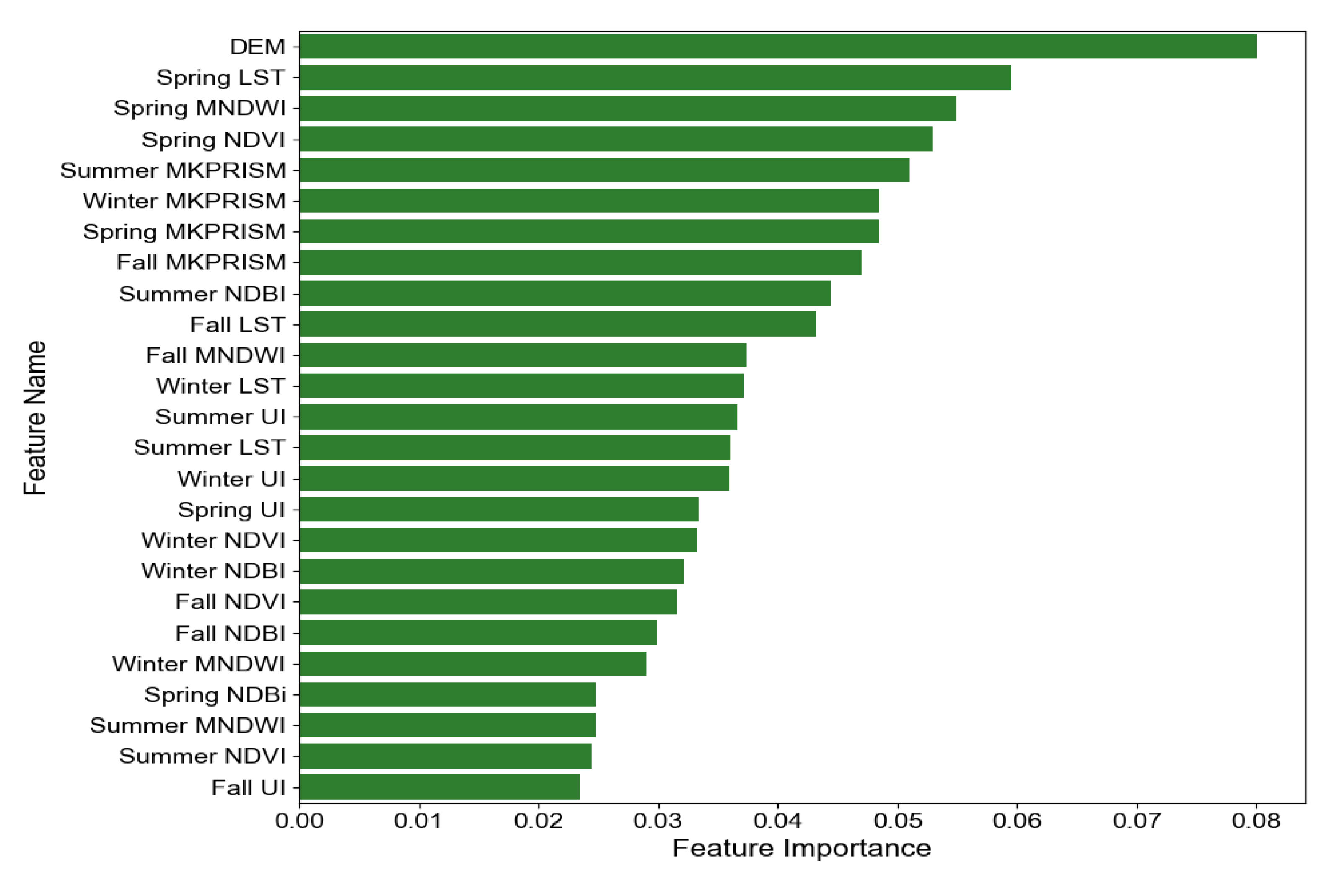
Table 1. Variables derived from Landsat imagery for EFG classification model.

Indices	Formula
Normalized Difference Vegetation Index (NDVI)	$(ρ_{N I R} - ρ_{R E D}) / (ρ_{N I R} + ρ_{R E D})$
Modified Normalized Difference Water Index (MNDWI)	$(ρ_{G R E E N} - ρ_{S W I R 1}) / (ρ_{G R E E N} + ρ_{S W I R 1})$
Normalized Difference Built-up Index (NDBI)	$(ρ_{S W I R 1} - ρ_{N I R}) / (ρ_{S W I R 1} + ρ_{N I R})$
Urban Index (UI)	$(ρ_{S W I R 2} - ρ_{N I R}) / (ρ_{S W I R 2} + ρ_{N I R})$
Land Surface Temperature (LST)	$ρ_{T I R}$

Table 2. Accuracy measures used to assess RF classification model.

Approach	Formula
Overall accuracy	T / (T+F)
Precision	TP / (TP+FP)
Recall	TP / (TP+FN)
F1-score	(2×precision×recall) / (precision+ recall)

Disclaimer/Publisher’s Note: The statements, opinions and data contained in all publications are solely those of the individual author(s) and contributor(s) and not of MDPI and/or the editor(s). MDPI and/or the editor(s) disclaim responsibility for any injury to people or property resulting from any ideas, methods, instructions or products referred to in the content.

© 2025 by the authors. Licensee MDPI, Basel, Switzerland. This article is an open access article distributed under the terms and conditions of the Creative Commons Attribution (CC BY) license (http://creativecommons.org/licenses/by/4.0/).

Copyright: This open access article is published under a Creative Commons CC BY 4.0 license, which permit the free download, distribution, and reuse, provided that the author and preprint are cited in any reuse.