Submitted:
15 April 2025
Posted:
16 April 2025
You are already at the latest version
Abstract
Native forests provide forage for grazing animals. We investigated whether native and exotic vegetation promotes potential animal load (PAL, ind ha-1 yr-1) for cattle (Bos taurus, ~700 kg) and sheep (Ovis aries, ~60 kg) in contrasting native forest types and canopy cover (closed, semi-open, open). The study was conducted in Chilean Patagonia (-44° to -49° SL). Vegetation cover (%) and growth habit data (trees, shrubs, forbs, graminoids, ferns, lianas, lichens, and bryophytes) were collected from 374 plots (up to 5 ha) representing the following types: coihue (Nothofagus dombeyi, CO), lenga (N. pumilio, LE), mixed Nothofagus forests (MI), ñire (N. antarctica, ÑI), evergreen forests (SV), and open-lands (OL). We combine this data with bibliographic research and laboratory analyses (e.g. crude protein, %) to develop PAL values for the year's four seasons. Data were evaluated using descriptive statistical analyses, ANOVAs, and Multiple Correspondence Analysis. The analyses indicated that closed forests exhibited a greater percentage of native species (~56.6%) compared to opened forests (~33.3%), while OL had the highest coverage of exotic species (~68.6%). LE was forest type with major native species coverage (~58.0%), whereas ÑI forests had the highest exotic cover (~53.0%). The closed forests had fewer exotic species than semi-open and open forests, which supported a higher cover of native and exotic plants (p <0.01). Forbs were the dominant growth habit in closed forests, while graminoids were more common in OL (~45.8%). The multivariate analysis showed that LE and CO forest types and closed canopy cover were associated with lower PAL values, explaining 91.2% of the variance. Our analysis also showed that exotic species predominated environment types with high PAL, particularly during spring and summer when cover increased. This indicates a trade-off between forage production in the forest and the presence of exotic plants.
Keywords:
native forests
; livestock grazing
; potential animal load
; exotic vegetation
; Patagonia
1. Introduction
There is worldwide interest in integrating sustainable forest management and maintaining biodiversity, giving rise to the controversial divide between integration and separation of conservation with production systems. In a separation scenario, the available land is divided into areas focused on maximizing productive capacity (e.g. intensive livestock farming), while other areas are dedicated to maintaining biodiversity. In an integration scenario, a lower production level is maintained in exchange for biodiversity to be conserved throughout the landscape [1].
Native forests are vital by providing multiple ecosystem services for the people [2,3]. These services are diverse, including biodiversity, water regulation, and non-timber products (e.g. provision of forage), among others [4,5]. Forests and their goods and services (e.g. forage quality) largely depend on vegetation biodiversity [6,7]. Assessing how vegetation responds to integrating human uses is imperative to reconcile sustainable land use and biodiversity [8,9]. Then, vegetation changes are the starting point for research on land management from an integration perspective of the production system.
Evidence at regional and global scales showed that most species are declining because of human activities (losers) and are being replaced by far fewer expanding species that thrive in human-altered environments (winners) [10]. A few generalists’ replacements of numerous specialist species generate a biotic homogenization [10,11] that can reflect stable states (e.g. exotic plant species that dominate in cover). These changes can occur in native forests with integrated livestock [5,12,13]. Forest canopy openings influence the amount of light reaching the understory, which affects vegetation composition [14,15,16]. The degree of canopy cover can negatively impact some plant species, while others significantly increase their cover [17,18]. Previous studies suggest livestock can produce different effects on vegetation because of herbivore selectivity to specific plant species, e.g. cattle prefer grasses while sheep prefer legumes and other broadleaf species [19,20,21,22,23].
Native and exotic species coverage may depend not only on the forest’s structural and ecological processes but also on the associated open lands (e.g. grasslands and shrublands) [24,25], such as the entry of native or exotic species from surrounding environments [26,27]. Vegetation in different environment types (e.g. forest types or open-lands) can exhibit phenological stages (e.g. forage) throughout different seasons, which is a crucial factor in herbivory feeding [19,28,29,30]. Vegetation growth peaks in spring and summer across different environment types, while autumn and winter bring changes as vegetation enters senescence, during which domestic herbivores increase their consumption of forest vegetation (e.g. tree seedling, sapling, shrubs) [31]. In this context, revealing the role of native and exotic vegetation can provide a pathway in land integration for productive potential (e.g. livestock systems) in native forests. Here, we investigated the causal relationships between native and exotic vegetation cover (%) and the Potential Animal Load (PAL, ind ha-1 yr-1) for a common type of livestock worldwide (cattle and sheep) in contrasting native forests and canopy cover (closed, semi-open, open) in Chilean Patagonia. We hypothesize that vegetation’s origin and growth habits should differentially influence homogenization on forage quality, consequently affecting the potential animal load and its integration in native forests.
2. Materials and Methods
2.1. Study Area
Our study area focused on the Aysén region (108,494 km²) in Chilean Patagonia between -44° and -49° SL. The research concentrated on the eastern side of the Andes, which is more suitable and accessible for livestock systems, with the Carretera Austral as the central road system (Figure 1). We excluded the western side due to its extensive protected areas (National Parks and Reserves), where agricultural development and livestock farming are mostly prohibited. The forests contain 18 predominant forest types featuring various tree species [32]. The genus Nothofagus is the most representative, including evergreen forests with N. dombeyi and N. betuloides and deciduous forests with species such as N. pumilio and N. antarctica. The climate is warm temperate mesothermal, varying by location and elevation. Precipitation ranges from ±3,000 to ±4,000 mm yr-1 on the western side and ±500 to ±1,500 mm yr-1 on the eastern side. Summer temperatures (December to February) range between 10 and 18°C, while winter temperatures (June to August) drop below 0°C, with conditions including heavy rain, snow, and strong winds [33].
2.2. Sampling Design and Data Taking
We first explored potential study sites with native forests and open-lands using ArcGIS Desktop 10.8.2 [34]. We generated a set of 500 points randomly distributed on the CONAF land shapefile layer [35], which contains spatially explicit land-cover data for the study area. Then, ground-truthing was conducted at these points during the round year (four seasons) between 2022 and 2024. After field verification, we selected 374 plots representing the target native forest types and associated open-lands in ranches, national parks, and reserves. These plots (>5 ha) were homogeneous in composition and intensity of use. They were categorized into the following types: coihue (Nothofagus dombeyi, CO), lenga (N. pumilio, LE), mixed Nothofagus forests (MI), ñire (N. antarctica, ÑI), evergreen forests (SV), and open-lands (OL) composed by a combination of grasslands, shrublands and peatlands. In the forest plots, we measured the canopy cover using hemispherical photographs with a Nikon 35 mm digital camera (Nikon D800, Japan), a tripod at 1 meter up to the floor, and an 8 mm fisheye lens (Sigma, Japan). Photographs were oriented so that the top edge of the lens faced magnetic north, and direct sunlight was avoided. Gap Light Analyzer v.2.0 software [36] was used to analyze the photographs and calculate the percentage of forest canopy cover (CC). Using this data, we classified the plots as closed (>70% CC), semi-open (40% to 70% CC), and open (<40% CC) (Figure 2A).
Vegetation metrics were measured in 1.0 ha plots during the spring and summer (flowering period) to accurately identify species in each plot across the different environment types. Vegetation cover (%) was determined using the point-interception method (PIM) [37], with a 50-m transect marked at every meter (Figure 2B). Vegetation was classified by plant origin (native or exotic) and growth habit (trees, shrubs, forbs, graminoids, ferns, lianas, lichens, and bryophytes), including coarse woody debris and bare soil. The plants were sampled for subsequent chemical composition analyses using a 0.5 m² quadrant randomly placed at each plot. All plants within the quadrant were collected at the base, labelled with location, site identification number, and sampling date, and transported to the laboratory promptly. In the laboratory, plants were analyzed using gravimetric destructive random sampling (kg dry matter ha-1), weighed with an analytical balance (±0.0001 g) (Boeco, Germany), and dried in an oven at 60°C (Binder, USA) until constant weight. Plant nitrogen content was measured using the LECO TruSpec® CHN simultaneous elemental determinator (USA) with the Dumas direct combustion method (Figure 2C). Following AOAC [38], plant nitrogen content (% and mg) was used to calculate crude protein (CP, % dry matter) by multiplying it by a factor of 6.25. Nitrogen percentage measurements were obtained for each analyzed season (summer, autumn, spring, and winter), resulting in distinct CP values for each plant species.
2.3. Plant Nutritional Data Approach
We propose the following indices to analyze the plant nutritional quality [39]: (i) Crude protein index (CPI) based on average CP levels (Figure 2C) as follows: 0-10% (very low CP), 10-12% (low CP), 12-15% (medium CP), 15-18% (high CP), and >18% (very high CP). (ii) Phenological index (PHI) (Figure 2D), where plant phenological stages were classified and rated (rPHI) as follows: absent (rPHI = 0.00) when plant species was not available, 0 (rPHI = 0.25) when plant species occurred at the beginning or the end of the growing phase, intermediate stage (rPHI = 0.50) when plant species was fruiting or drying; near-complete development (rPHI = 0.75) when plant species was near to or continuing flowering; and complete development (rPHI = 1.00) when plant species was at maximum flowering expression. (iii) Specific quality index (SQI) was calculated following Daget and Poissonet [40] (Figure 2D), which considered plant phenology, palatability, and potential assimilability by ruminants, considering the specific quality values (SQ) ranging from 0 (no animal interest) to 10 (maximum animal interest). For the study area validation, we compared our SQI indices with those defined in other studies [5,40,41].
These indices were used to calculate a pastoral value index (PVI), which integrates all the information of plant composition (Figure 2E). PVI provides insights into pasture quality by ranking the importance of plant species based on their zootechnical interest, vegetation composition, and plant understory cover (%). The index ranges from 0 (environments with no zootechnical value) to 100 (environments of maximum zootechnical relevance). We used PVI as a proxy for the plot’s potential animal load (PAL), following Daget and Poissonnet [40]. This approach assumes that one livestock unit (LU) requires one specific number of milk forage unit (MFU) per year. Also, PAL included 0.02 PVI for European standard cattle (Bos taurus, ~700 kg) consuming a total of 3,000 MFU yr-1. Finally, we calculated the potential forage production (PFP) as x = PVI × 0.2 × 3,000, reflecting the plot’s output in MFU ha-1 yr-1. We calculated these values for all the plots, where cattle required 2,555 MFU yr-1, and sheep required 292 MFU yr-1. This rationale was used to determine the final data of potential animal load (PAL) (Figure 2E) following Daget and Poissonnet [40] and INRA [39]. PAL was calculated as PFP/2,555 for cattle, resulting in an average value of 0.023 PVI (PAL cattle, ind ha-1 yr-1). The sheep (Ovis aries) calculation was based on PFP/292, achieving to 0.205 PVI (PAL sheep, ind ha-1 yr-1). We utilized PAL values as focus data for our analyses (cattle and sheep) across different seasons. For better interpretation of these data, PAL values were classified into: (A) For sheep: <1.0 (low), 1.0-5.0 (medium), and >5.0 (high), and (B) for cattle: <0.3 (low), 0.3-1.0 (medium), and >1.0 (high).
2.4. Data Analyses
We quantified the occurrence frequency of plants (%) at each interception point (Table A1), and we standardized these values on a scale from 0 to 100 to calculate vegetation cover. One-way ANOVAs were used to highlight how vegetation and ground cover varied between native and exotic species, and across different environment types (CO, LE, MI, ÑI, SV, OL) and canopy cover (closed, semi-open, open, compared to OL) as main factors. PAL values for sheep and cattle were also analyzed using one-way ANOVAs to link vegetation quality and its seasonal variability, comparing environment types and canopy cover as main factors. We calculated ratios for PAL values to visualize variations of each factor across the different seasons. The variables were log-transformed to meet ANOVA assumptions, which were assessed using the Shapiro-Wilk and Levene tests; however, non-transformed means were presented. Comparisons of the means were conducted using Tukey post-hoc test (p <0.05). These analyses were performed using Statgraphics Centurion XVI Version 16.1.11 (StatPoint Technologies, Warrenton, USA). Finally, we conducted two multiple correspondence analysis (MCAs): (i) The first one analyzed the association between environment types and canopy cover with PAL for sheep and cattle. (ii) The second one aimed to detect the factors related to variations in canopy cover (%) of native and exotic plant species across the forest types, using PAL values during the growing season (spring and summer). Both MCAs were performed in R using the FactoMineR (Version 2.11) library following Lê et al. [42].
3. Results
A total of 163 species were surveyed, 73% natives and 27% exotic, where the most frequent growth habit was forb (45%), shrub (21%), and graminoid (17%). When we analyzed vegetation cover (%) by plant origin and growth habit across the different environment types, ANOVAs showed that native species predominated most forest types (~45%), particularly in the LE forest (~58%). In contrast, exotic species increased in ÑI and OL (p <0.01, Table 1). The CO, MI, and SV forest types exhibited more than 40% native species cover, with fewer exotic species. ÑI (~38%) and OL (~20%) displayed the lowest native species coverage. Exotic species had their highest coverage in ÑI (~53%), like OL (~68%). ÑI was the only forest type where exotic species exceeded native species, while LE had the lowest exotic species cover (~16%). Graminoids dominated the OL and ÑI regarding growth habits, covering 44% and 30%, respectively. Others forest types primarily comprise forbs, shrubs, and tree ground cover (e.g. natural forest regeneration). Ferns contributed around 5% of the total cover in the studied environments, while mean cover of bryophytes were significant for CO which reached nearly 8% coverage. ÑI and OL showed over 90% ground coverage by vegetation, with lower proportions of woody debris or bare soil than other forest types. In contrast, woody debris covered over 20% in LE and CO, while SV exhibited similar coverage of woody debris and bare soil.
ANOVAs also indicated that the degree of forest canopy cover resulted in a variation in the understory cover of native and exotic species (Table 2). The growth habits of understory species in OL differed from open or semi-open forests, as OL doubled the coverage percentage of exotic species (p <0.01). In contrast, native species dominated closed forests, covering over 55% of the ground. Graminoids primarily covered OL and semi-open forests more than open forests and were less prevalent in closed forests. Forbs predominated in closed forests, followed by shrubs, while other coverage consisted of woody debris, which accounted for over 20% of ground cover. Forbs were the dominant growth habit in open and semi-open forests, greater than graminoids. Open forest types had 26% of bare soil cover, while closed forests had only 2.4%. All canopy cover categories exhibited less total vegetation coverage than OL.
Differences in PAL among forest types and OL were similar for sheep and cattle, with no significant differences compared to the mean for sheep and forest types (Figure 3). However, PAL values significantly differed across forest types (p <0.01). ÑI showed PAL similarities with OL, unlike LE and CO types which markedly decreased. MI forest types were almost equal to the total mean values. Besides, PAL values diminished in summer, being marked in autumn and winter. Canopy cover significantly (p <0.01) affected PAL of cattle and sheep in the analyzed environment types (forests vs OL) (Figure 4). In spring, OL had higher PAL compared to forests with varying levels of canopy cover. Semi-open and open forest types showed a more similar group to OL, and dissimilar in terms of PAL from closed forests. These differences were more evident for sheep, where PAL in closed forests was lower than any level of forest cover and especially lower than in OL. In contrast, for cattle, although significant differences were observed among the various canopy cover levels in spring (p <0.01), these differences were almost equal to the total mean among the groups.
First MCA showed that environment types, forest canopy cover, and PAL (sheep and cattle) were closely related (Figure 5). Axis 1 (eigenvalue = 0.527, horizontal line) and Axis 2 (eigenvalue = 0.141, vertical line) explained 98.6% of the cumulative variance of the model. Axis 1 alone explained 91.2% of data variation, presenting the highest inertia (λ = 0.278). MCA model revealed discrimination between axes, where LE and CO forest types and the closed canopy cover categories contributed most to the lowest PAL values across different seasons for both sheep and cattle. Besides, SV was close to the origin of Axes 1 and 2, which was associated with medium PAL values. ÑI and MI forest types contributed to the middle PAL values, as well as open and semi-open canopy covers. In contrast, OL differed from the other environment types and canopy cover categories, comprising and grouping the highest PAL values for all the seasons and livestock types (sheep and cattle). Second MCA highlighted the relationship between PAL and understory cover of native and exotic species (Figure 6). Axis 1, with an eigenvalue of 0.959, explained 48.6% of the cumulative variance, exhibiting the highest inertia (λ = 0.921), while Axis 2, with an eigenvalue of 0.859, contributed with an inertia of 0.738. This resulting in a cumulative percentage variance of 87.6% when both axes were considered. This second MCA conformed to a conspicuous group of low PAL associated with high cover percentages of native species (indicated by green numbers), which emphasizing the disparity in the cover between native and exotic species, and high PAL values for cattle and sheep.
4. Discussion
4.1. Plant Origins and Growth Habits
Our research showed different plant origin and growth habit types in the different forest types and OL that we studied, with varying amounts of native and exotic species. It is expected that several species introduced in Patagonia were intended primarily for ruminant foraging (e.g. Taraxacum officinale, Dactylis glomerata, Holcus lanatus), with a few designated for human consumption (e.g. Rosa eglanteria) or aesthetic purposes (e.g. Lupinus polyphyllus). The dominance of native species in LE forests align with expected less disturbed ecosystems, emphasizing the resilience of native species in closed canopy stands. In contrast, the high exotic species cover in ÑI and OL suggests a correlation between canopy cover and plant invasion vulnerability, generating significant environment homogenization. This supports previous findings that land-sharing, such as logging or grazing, often promotes the establishment of exotic species [27]. Previous studies have indicated the connection between plant composition and the diversity of structures in these native forests [25]. Preserving diverse canopy structures is crucial for maintaining plant diversity [15,16,43]. Plants are essential for energy transfer and nutrient cycling in ecosystems [44] and respond in complex ways to natural and human-induced disturbances [6]. Then, various factors, such as species-specific autecology, canopy structure and composition, site and microsite conditions, and interactions with dominant trees, shape plant abundance and distribution [45,46,47]. Besides, the variation in growth habits in the studied environments highlights the structural shifts in plants in response to integrated natural forests with livestock conditions. The higher exotic species cover in more open environments highlights the vulnerability of these areas to exotic species. The reduced bare soil cover in closed forests suggests healthier soil conditions, while the increase in bare soil in open environments indicates degradation processes, such as erosion. This raises concerns about how further canopy disturbances could alter these dynamics, potentially decreasing forest resilience. Light availability within the forest is essential, influenced by tree density and canopy cover [48]. The forest type also plays a significant role, where deciduous trees shedding their leaves in autumn create high seasonal variation in light availability for understory plants. On the other hand, evergreen trees maintain their leaves year-round, leading to a need for plants to adapt to low light conditions throughout the year [14,15,16]. The differences in understory plant communities across different forest types underscore the need for tailored conservation strategies considering local conditions and species distributions [49].
4.2. Nutritional Subsidies for Grazing Animals
We found associations between factors (environment types and canopy cover) and the low, medium, and high Potential Animal Load (PAL). The marked differences in PAL across the different environments reveal the significant pressure livestock exerts on ÑI and OL, especially during autumn and winter when plant regeneration is slower. The fact that PAL is lowest in LE and CO forests highlights the protective role of intact forest canopies in limiting grazing pressure. Here, we showed the relationships between PAL, forest types, and species composition. Our data reveal that OL consistently supports higher PAL ratios for sheep and cattle than in forested areas, notably closed forests. For sheep, restricted grazing opportunities in certain forest types, especially LE, indicate a need for management strategies that optimize livestock foraging while conserving native biodiversity. Cattle, however, display greater adaptability, utilizing forage across various environments with only minor differences in PAL. Additionally, the PAL is often associated with high native species coverage, indicating that as livestock pressure increases, native species are likely to be displaced by exotic species, particularly in open and semi-open forest settings. In this context, analyzed environments provide pivotal understory species to support livestock forage [7]. This extensive activity involves cattle and sheep species and combines native forests with open grasslands [22,50,51]. However, previous studies indicate that livestock grazing changes understory plant communities within these forests (e.g. dominance in coverage of native or exotic species) [25]. Pointing out that developing forests managed for livestock use raises questions about their forest ecological perspective to promote a balance between productive alternatives and ecological values [52]. In forests with livestock uses (e.g. silvopastoral systems), the plant forage value and animal occurrence varied significantly across management alternatives and associated environments [13]. Prior work suggests that habitat diversity plays a crucial role in shaping the dietary patterns of herbivores. Soler et al. [53] found that the diverse habitats and plant species within Nothofagus forests significantly influence the seasonal dietary patterns of native mammals. Moreover, different authors [4,5,22,25,51] underscores the importance of understanding the varying responses of forage production to environmental drivers (e.g. droughts) in different systems, as this knowledge can inform management practices that improve the resilience of livestock production in the face of increasing climate variability. Considering the phenological stage is also essential when evaluating plant availability for livestock feeding, as different species have distinct growing times, affecting their accessibility to livestock throughout the year (Figure 3 and 4). Previous studies show that both palatable and non-palatable plants, whether dead or alive, present estimations of change and nutritional contributions [31]. Our data highlights that the plant exotic component is fundamental to understanding the forage potential of the studied forests and associated OL.
4.3. Limitations of the Present Study
It is commonly believed that the autumn and winter seasons are critical for the functionality of these landscapes (Figure 7), at least in terms of nutritional offerings to support sheep and cattle, the main livestock species. We found that analyzed exotic species contribute to the forage potential of the studied forests, underscoring the complex interplay between native and exotic vegetation in the studied environment types. This is fundamental because animals can rely on this food availability during scarcity or winter. In this context, winter and the forest type are essential in managing the forest with livestock use. For this reason, some species acquire greater importance, as they are available during these periods. Moreover, other components like lichens appear, which animals may utilize as food; this ultimately becomes an essential component during winter in the forests.
Clarifying our findings to provide practical management recommendations is crucial. Although there are evident changes due to climate shifts across the seasons, where snow plays a vital role in the functionality of the different forest and environment types, plants can still be utilized for human interests, such as animal nutrition. The idea is that these environment types can offer differentiated functionalities throughout the seasons, providing multiple benefits of interest for human production systems, such as livestock. Here, we compare the potential productivity of native forests from a global perspective, contrasting Patagonia forests with highly productive systems such as grasslands, primarily composed of exotic species used in productive systems worldwide as forage for livestock. In this context, our results, obtained through an approach that used a developed index of potential forage for the studied environment types, demonstrate the comparability of these environment types with others worldwide using standardized parameters, e.g. for cattle 700 kg and for sheep 60 kg. This means all the environment types that we analyzed can support livestock production, though some more effectively than others, such as OL and ÑI forest types. The other environments can also support animal forage, although our study did not consider cattle or sheep age classes (e.g. calf, yearling, heifer, cow, lamb) or smaller livestock species (e.g. goat, pig, chicken).
5. Conclusions
Our hypothesis supported the idea that the differential influence of native and exotic vegetation affects forage quality and its impact on potential animal load. Closed native forests are unsuitable for livestock forage; therefore, it is advisable to conserve them in their current state to maintain other ecosystem services. Promoting closed canopies can enhance the coverage of native species while limiting the growth of exotic species. While seasonal changes influence potential animal load, the specific environment type and canopy cover are critical factors. Enhancing forage production for livestock often necessitates the introduction of exotic plant species, which can support a higher potential animal load. This situation suggests a trade-off between forage production within the forest and the prevalence of exotic plants. After all, here we showed that in native forests with integrated livestock, exotic “winners” can homogenize diverse environment types for production systems.
References
Author Contributions
Conceptualization, T.B., M.D.R.T.M., A.H.H.; methodology, T.B., A.B., G.M.P., A.H.H.; software, A.B., P.J.M.G., L.L.; validation, S.V.C., S.M.M.; formal analysis, T.B., M.D.R.T.M., G.M.P., A.H.H.; investigation, T.B.; resources, A.B., P.J.M.G., L.L.; data curation, A.B., S.V.C.; writing-original draft preparation, T.B., A.B., M.D.R.T.M., A.H.H.; writing, review and editing, S.V.C., P.J.M.G. , L.L. , G.M.P., S.M.M.; visualization, A.B., P.J.M.G. , L.L.; supervision and project administration, M.D.R.T.M., A.H.H.; funding acquisition, M.D.R.T.M., A.H.H. All authors have read and agreed to the published version of the manuscript.
Funding
No funding to inform.
Data Availability Statement
Availability of data and material: At CADIC-CONICET (Argentina) repository. The data supporting this study’s findings are available from the corresponding author upon reasonable request.
Acknowledgments
We thank the Centro de Investigación en Ecosistemas de la Patagonia (CIEP), the Gobierno Regional de Aysén (GORE Aysén), FNDR BIP 40047145-0, ANID Regional R20F0002, ANID FONDEQUIP EQM220096, the Ecole National Vétérinaire de Toulouse (ENVT) and the Université de Pau et des Pays de l’Adour (UPPA), the Centro Austral de Investigaciones Científicas (CADIC-CONICET), and the Regional Ministry of Innovation, Universities, Science and Digital Society of the Generalitat Valenciana (CIGE/2023/12) for their financial support and encouragement of our work. We want to thank Rosa Torres and Ricardo Ulloa for their support in processing laboratory samples. We also thank CONAF-Aysén, the forestry and ranching producers of the Aysén region.
Conflicts of Interest
The authors declare no conflict of interest. The funders had no role in the design of the study; in the collection, analyses, or interpretation of data; in the writing of the manuscript, or in the decision to publish the results.

Table A1.
Occurrence of understory plants (%) in the studied environment types (CO = coihue, LE = lenga, MI = mixed, ÑI = ñire, SV = evergreen, OL = open-lands) and forest canopy cover (closed, semi-open, open).
Table A1.
Occurrence of understory plants (%) in the studied environment types (CO = coihue, LE = lenga, MI = mixed, ÑI = ñire, SV = evergreen, OL = open-lands) and forest canopy cover (closed, semi-open, open).
| Code | Species | Origin | Growth Habit | Environment Type | Total | Canopy Cover | Total | |||||||
| CO | LE | MI | ÑI | SV | OL | Closed | Semi-open | Open | ||||||
| ACIN | Acaena integerrima | Native | Forb | 0.0 | 0.5 | 0.0 | 1.3 | 0.3 | 1.3 | 3.5 | 0.4 | 1.8 | 0.7 | 2.9 |
| ACMA | Acaena magellanica | Native | Forb | 0.0 | 1.1 | 0.0 | 0.0 | 0.0 | 0.8 | 1.9 | 1.1 | 0.4 | 0.0 | 1.4 |
| ACMI | Achillea millefolium | Exotic | Forb | 0.0 | 1.6 | 0.3 | 5.1 | 0.0 | 7.5 | 14.4 | 3.6 | 5.4 | 0.4 | 9.4 |
| ACOV | Acaena ovalifolia | Native | Forb | 2.7 | 15.2 | 3.2 | 8.8 | 2.4 | 5.6 | 38.0 | 30.1 | 12.7 | 1.1 | 43.8 |
| ACPI | Acaena pinnatifida | Native | Forb | 1.3 | 6.4 | 1.1 | 9.1 | 0.0 | 2.7 | 20.6 | 9.4 | 13.0 | 1.8 | 24.3 |
| ADCH | Adenocaulon chilense | Native | Forb | 2.4 | 17.6 | 1.9 | 4.3 | 0.0 | 0.5 | 26.7 | 29.7 | 5.4 | 0.4 | 35.5 |
| AGCA | Agrostis capillaris | Exotic | Graminoid | 0.5 | 6.1 | 0.0 | 5.9 | 0.0 | 12.6 | 25.1 | 8.0 | 8.3 | 0.7 | 17.0 |
| AGLE | Agrostis leptotricha | Native | Graminoid | 0.0 | 0.0 | 0.0 | 0.3 | 0.0 | 0.0 | 0.3 | 0.0 | 0.4 | 0.0 | 0.4 |
| AGST | Agrostis stolonifera | Exotic | Graminoid | 0.0 | 0.3 | 0.3 | 2.9 | 0.5 | 1.1 | 5.1 | 1.8 | 3.3 | 0.4 | 5.4 |
| AICA | Aira caryophyllea | Exotic | Graminoid | 0.3 | 0.3 | 0.0 | 1.1 | 0.0 | 4.3 | 5.9 | 0.0 | 1.8 | 0.4 | 2.2 |
| AMLU | Amomyrtus luma | Native | Tree | 0.5 | 0.0 | 0.3 | 0.0 | 0.8 | 0.0 | 1.6 | 1.4 | 0.7 | 0.0 | 2.2 |
| ANOD | Anthoxanthum odoratum | Exotic | Graminoid | 0.0 | 0.0 | 0.0 | 2.4 | 0.0 | 0.0 | 2.4 | 1.8 | 1.4 | 0.0 | 3.3 |
| ANMU | Anemone multifida | Native | Forb | 0.0 | 4.0 | 0.8 | 10.2 | 0.3 | 1.1 | 16.3 | 6.9 | 12.3 | 1.4 | 20.7 |
| ARCH | Aristotelia chilensis | Native | Tree | 0.0 | 0.3 | 0.0 | 0.0 | 0.3 | 0.5 | 1.1 | 0.7 | 0.0 | 0.0 | 0.7 |
| ARMA | Armeria maritima | Native | Forb | 0.0 | 0.0 | 0.0 | 0.0 | 0.0 | 0.3 | 0.3 | 0.0 | 0.0 | 0.0 | 0.0 |
| AZLA | Azara lanceolata | Native | Tree | 2.7 | 0.3 | 0.5 | 0.0 | 2.1 | 0.0 | 5.6 | 5.8 | 1.8 | 0.0 | 7.6 |
| BAMA | Baccharis magellanica | Native | Shrub | 0.0 | 1.3 | 0.8 | 5.3 | 0.0 | 0.8 | 8.3 | 3.6 | 5.8 | 0.7 | 10.1 |
| BEDA | Berberis darwinii | Native | Shrub | 2.1 | 5.1 | 1.6 | 4.0 | 1.6 | 7.2 | 21.7 | 12.7 | 6.2 | 0.7 | 19.6 |
| BEEM | Berberis empetrifollia | Native | Shrub | 0.0 | 0.3 | 0.0 | 0.3 | 0.0 | 0.0 | 0.5 | 0.0 | 0.4 | 0.4 | 0.7 |
| BEMI | Berberis microphylla | Native | Shrub | 1.9 | 6.1 | 0.8 | 17.6 | 0.8 | 5.3 | 32.6 | 18.8 | 16.7 | 1.4 | 37.0 |
| BESE | Berberis serratodentata | Native | Shrub | 0.3 | 3.7 | 0.5 | 0.3 | 0.3 | 0.0 | 5.1 | 6.5 | 0.4 | 0.0 | 6.9 |
| BLMO | Blechnum mochaenum | Native | Fern | 0.3 | 0.0 | 0.0 | 0.0 | 0.3 | 0.0 | 0.5 | 0.7 | 0.0 | 0.0 | 0.7 |
| BLCL | Blechnum chilense | Native | Fern | 0.3 | 0.0 | 0.0 | 0.0 | 0.5 | 0.0 | 0.8 | 1.1 | 0.0 | 0.0 | 1.1 |
| BLPE | Blechnum pennamarina | Native | Fern | 4.5 | 12.3 | 2.4 | 13.9 | 2.1 | 9.1 | 44.4 | 33.3 | 14.1 | 0.4 | 47.8 |
| BRSE | Bromus setifolius | Native | Graminoid | 0.3 | 5.9 | 0.3 | 0.5 | 0.0 | 0.3 | 7.2 | 7.2 | 2.2 | 0.0 | 9.4 |
| BRUN | Bromus unioloides | Native | Graminoid | 0.0 | 0.8 | 0.0 | 0.0 | 0.0 | 0.5 | 1.3 | 1.1 | 0.0 | 0.0 | 1.1 |
| CABI | Calceolaria biflora | Native | Forb | 0.0 | 2.1 | 0.0 | 2.9 | 0.0 | 0.0 | 5.1 | 2.2 | 4.0 | 0.7 | 6.9 |
| CAVA | Capsidium valdivianum | Native | Liana | 0.3 | 0.0 | 0.0 | 0.0 | 0.5 | 0.0 | 0.8 | 1.1 | 0.0 | 0.0 | 1.1 |
| CABA | Carex banksii | Native | Graminoid | 0.0 | 0.0 | 0.0 | 2.7 | 0.0 | 0.5 | 3.2 | 2.2 | 1.4 | 0.0 | 3.6 |
| CADA | Carex darwinii | Native | Graminoid | 0.3 | 0.3 | 0.0 | 0.3 | 0.0 | 2.4 | 3.2 | 0.4 | 0.7 | 0.0 | 1.1 |
| CAFU | Carex fuscula | Native | Graminoid | 0.0 | 0.0 | 0.0 | 1.1 | 0.0 | 0.3 | 1.3 | 0.4 | 1.1 | 0.0 | 1.4 |
| CAGA | Carex gayana | Native | Graminoid | 0.0 | 0.0 | 0.0 | 0.5 | 0.0 | 0.5 | 1.1 | 0.0 | 0.7 | 0.0 | 0.7 |
| CEAR | Cerastium arvense | Exotic | Forb | 0.0 | 4.0 | 0.8 | 8.3 | 0.0 | 1.9 | 15.0 | 5.4 | 10.5 | 1.8 | 17.8 |
| CEGL | Cerastium glomeratum | Exotic | Forb | 0.3 | 1.6 | 0.3 | 4.0 | 1.1 | 3.5 | 10.7 | 4.7 | 5.1 | 0.0 | 9.8 |
| CHCU | Chusquea culeou | Native | Shrub | 2.4 | 1.9 | 0.3 | 1.1 | 2.4 | 0.5 | 8.6 | 8.0 | 2.9 | 0.0 | 10.9 |
| CHDI | Chiliotrichum diffusum | Native | Shrub | 0.0 | 4.3 | 0.0 | 3.2 | 0.0 | 1.1 | 8.6 | 5.8 | 4.0 | 0.4 | 10.1 |
| CIVU | Cirsium vulgare | Exotic | Shrub | 0.5 | 1.1 | 0.0 | 2.1 | 0.5 | 0.5 | 4.8 | 2.5 | 3.3 | 0.0 | 5.8 |
| COBI | Collomia biflora | Native | Forb | 0.0 | 0.0 | 0.0 | 1.1 | 0.0 | 0.0 | 1.1 | 0.0 | 1.4 | 0.0 | 1.4 |
| COES | Colletia spinosa | Native | Shrub | 0.0 | 0.0 | 0.0 | 0.0 | 0.3 | 0.0 | 0.3 | 0.0 | 0.4 | 0.0 | 0.4 |
| COHY | Colletia hystrix | Native | Shrub | 0.0 | 0.0 | 0.0 | 1.1 | 0.0 | 0.0 | 1.1 | 0.0 | 1.1 | 0.4 | 1.4 |
| COIN | Colliguaja integerrima | Native | Shrub | 0.0 | 0.0 | 0.0 | 0.0 | 0.5 | 0.0 | 0.5 | 0.0 | 0.4 | 0.4 | 0.7 |
| COLE | Codonorchis lessonii | Native | Forb | 0.3 | 4.8 | 0.3 | 0.0 | 0.0 | 0.3 | 5.6 | 6.9 | 0.4 | 0.0 | 7.2 |
| CRCA | Crepis capillaris | Exotic | Forb | 1.1 | 0.8 | 0.0 | 3.5 | 0.0 | 3.5 | 8.8 | 2.5 | 4.3 | 0.4 | 7.2 |
| DAGL | Dactylis glomerata | Exotic | Graminoid | 0.5 | 7.2 | 0.8 | 8.3 | 2.1 | 13.9 | 32.9 | 9.8 | 14.5 | 1.4 | 25.7 |
| DEDE | Dendroligotrichum dendroides | Native | Bryophyte | 0.0 | 0.0 | 0.3 | 0.3 | 0.3 | 0.0 | 0.8 | 0.7 | 0.0 | 0.4 | 1.1 |
| DICH | Discaria chacaye | Native | Shrub | 0.0 | 0.0 | 0.0 | 3.5 | 0.0 | 0.0 | 3.5 | 1.8 | 2.9 | 0.0 | 4.7 |
| DIPA | Diplolepis pachyphylla | Native | Liana | 0.3 | 0.0 | 0.0 | 0.0 | 0.0 | 0.0 | 0.3 | 0.4 | 0.0 | 0.0 | 0.4 |
| DIPU | Digitalis purpurea | Exotic | Forb | 0.5 | 0.0 | 0.0 | 0.0 | 0.3 | 0.0 | 0.8 | 0.7 | 0.4 | 0.0 | 1.1 |
| DRVE | Draba verna | Exotic | Forb | 0.0 | 0.0 | 0.0 | 1.6 | 0.0 | 0.0 | 1.6 | 0.7 | 1.4 | 0.0 | 2.2 |
| DRWI | Drimys winteri | Native | Tree | 0.3 | 0.0 | 0.0 | 0.0 | 0.5 | 0.0 | 0.8 | 1.1 | 0.0 | 0.0 | 1.1 |
| DYGL | Dysopsis glechomoides | Native | Forb | 0.5 | 1.6 | 0.3 | 0.8 | 0.5 | 0.3 | 4.0 | 2.9 | 1.8 | 0.4 | 5.1 |
| ECVU | Echium vulgare | Exotic | Forb | 0.0 | 0.0 | 0.3 | 0.3 | 0.0 | 0.8 | 1.3 | 0.4 | 0.4 | 0.0 | 0.7 |
| ELAN | Elymus angulatus | Native | Graminoid | 0.0 | 0.0 | 0.0 | 1.3 | 0.0 | 0.0 | 1.3 | 1.1 | 0.7 | 0.0 | 1.8 |
| ELPA | Eleocharis pachycarpa | Native | Graminoid | 0.0 | 0.8 | 0.0 | 0.0 | 0.0 | 0.0 | 0.8 | 1.1 | 0.0 | 0.0 | 1.1 |
| ELRE | Elymus repens | Exotic | Graminoid | 0.0 | 0.0 | 0.0 | 0.3 | 0.0 | 0.0 | 0.3 | 0.0 | 0.4 | 0.0 | 0.4 |
| EMCO | Embothrium coccineum | Native | Tree | 0.8 | 0.3 | 0.0 | 0.3 | 0.0 | 0.0 | 1.3 | 0.7 | 1.1 | 0.0 | 1.8 |
| EMRU | Empetrum rubrum | Native | Shrub | 0.0 | 0.8 | 0.0 | 2.7 | 0.0 | 0.5 | 4.0 | 2.9 | 1.8 | 0.0 | 4.7 |
| ESAL | Escallonia alpina | Native | Shrub | 0.0 | 0.0 | 0.0 | 0.5 | 0.0 | 0.3 | 0.8 | 0.4 | 0.4 | 0.0 | 0.7 |
| ESRU | Escallonia rubra | Native | Shrub | 0.3 | 0.0 | 0.0 | 0.3 | 0.0 | 0.0 | 0.5 | 0.4 | 0.4 | 0.0 | 0.7 |
| ESVI | Escallonia virgata | Native | Shrub | 0.0 | 0.0 | 0.0 | 3.2 | 0.0 | 1.6 | 4.8 | 2.5 | 1.8 | 0.0 | 4.3 |
| FEMA | Festuca magellanica | Native | Graminoid | 0.3 | 4.5 | 0.3 | 1.3 | 0.0 | 0.3 | 6.7 | 6.2 | 2.5 | 0.0 | 8.7 |
| FEPA | Festuca pallescens | Native | Graminoid | 0.0 | 2.7 | 0.0 | 5.6 | 0.0 | 1.1 | 9.4 | 1.8 | 7.2 | 2.2 | 11.2 |
| FERU | Festuca rubra | Native | Graminoid | 0.0 | 0.3 | 0.0 | 2.1 | 0.0 | 5.3 | 7.8 | 0.4 | 2.9 | 0.0 | 3.3 |
| FRCH | Fragaria chiloensis | Native | Forb | 0.3 | 7.8 | 0.3 | 11.5 | 0.0 | 2.1 | 21.9 | 12.7 | 13.0 | 1.1 | 26.8 |
| FUMA | Fuchsia magellanica | Native | Shrub | 1.3 | 0.8 | 0.0 | 0.0 | 2.1 | 3.5 | 7.8 | 4.3 | 1.4 | 0.0 | 5.8 |
| GAAP | Galium aparine | Exotic | Forb | 0.0 | 0.3 | 0.0 | 1.3 | 0.0 | 0.0 | 1.6 | 1.4 | 0.7 | 0.0 | 2.2 |
| GAHY | Galium hypocarpium | Native | Forb | 0.3 | 1.6 | 0.3 | 0.8 | 0.0 | 2.4 | 5.3 | 1.4 | 2.5 | 0.0 | 4.0 |
| GALU | Gavilea lutea | Native | Forb | 0.3 | 4.3 | 0.0 | 1.3 | 0.0 | 0.3 | 6.1 | 6.5 | 1.4 | 0.0 | 8.0 |
| GAMU | Gaultheria mucronata | Native | Shrub | 2.4 | 9.9 | 0.8 | 4.8 | 0.0 | 7.5 | 25.4 | 17.4 | 6.2 | 0.7 | 24.3 |
| GERMA | Geranium magallanicum | Native | Forb | 1.1 | 5.1 | 0.0 | 5.6 | 0.0 | 5.1 | 16.8 | 9.1 | 6.5 | 0.4 | 15.9 |
| GEMO | Geranium molle | Exotic | Forb | 0.0 | 0.0 | 0.0 | 1.1 | 0.0 | 2.1 | 3.2 | 0.4 | 1.1 | 0.0 | 1.4 |
| GEUMA | Geum magellanicum | Native | Forb | 0.3 | 2.4 | 0.3 | 0.8 | 0.0 | 0.0 | 3.7 | 3.3 | 1.8 | 0.0 | 5.1 |
| GRRU | Griselinia ruscifolia | Native | Shrub | 1.1 | 0.0 | 0.0 | 0.0 | 0.8 | 0.0 | 1.9 | 2.2 | 0.4 | 0.0 | 2.5 |
| GRSP | Greigia sphacelata | Native | Forb | 0.0 | 0.0 | 0.0 | 0.0 | 0.0 | 0.3 | 0.3 | 0.0 | 0.0 | 0.0 | 0.0 |
| GUMA | Gunnera magellanica | Native | Forb | 0.0 | 2.1 | 0.8 | 0.3 | 0.0 | 0.0 | 3.2 | 3.6 | 0.7 | 0.0 | 4.3 |
| GUTI | Gunnera tinctoria | Native | Forb | 0.3 | 0.0 | 0.0 | 0.0 | 0.0 | 0.0 | 0.3 | 0.4 | 0.0 | 0.0 | 0.4 |
| HOLA | Holcus lanatus | Exotic | Graminoid | 2.1 | 8.0 | 3.2 | 21.7 | 1.6 | 21.9 | 58.6 | 22.1 | 26.4 | 1.1 | 49.6 |
| HYDE | Hymenophyllum dentatum | Native | Forb | 0.0 | 0.0 | 0.0 | 0.0 | 0.3 | 0.0 | 0.3 | 0.4 | 0.0 | 0.0 | 0.4 |
| HYRA | Hypochaeris radicata | Exotic | Forb | 3.2 | 4.0 | 0.5 | 8.8 | 1.1 | 16.3 | 34.0 | 8.3 | 14.9 | 0.7 | 23.9 |
| HYSE | Hydrangea serratifolia | Native | Liana | 0.3 | 0.0 | 0.0 | 0.0 | 0.5 | 0.0 | 0.8 | 1.1 | 0.0 | 0.0 | 1.1 |
| JUPR | Juncus procerus | Native | Graminoid | 0.5 | 0.3 | 0.0 | 1.1 | 0.0 | 1.6 | 3.5 | 0.4 | 2.2 | 0.0 | 2.5 |
| LAHA | Lagenophora harioti | Native | Forb | 0.3 | 2.1 | 0.3 | 0.0 | 0.8 | 0.0 | 3.5 | 4.0 | 0.7 | 0.0 | 4.7 |
| LAMA | Lathyrus magellanicus | Native | Forb | 0.0 | 0.0 | 0.0 | 2.1 | 0.3 | 0.0 | 2.4 | 1.1 | 2.2 | 0.0 | 3.3 |
| LAPH | Laureliopsis philippiana | Native | Tree | 0.3 | 0.0 | 0.0 | 0.0 | 0.0 | 0.0 | 0.3 | 0.4 | 0.0 | 0.0 | 0.4 |
| LESC | Leptinella scariosa | Native | Forb | 0.5 | 0.5 | 0.0 | 0.0 | 0.8 | 4.8 | 6.7 | 1.1 | 1.4 | 0.0 | 2.5 |
| LETH | Leucheria thermarum | Native | Forb | 0.0 | 0.3 | 0.0 | 0.0 | 0.0 | 0.0 | 0.3 | 0.4 | 0.0 | 0.0 | 0.4 |
| LEVU | Leucanthemum vulgare | Exotic | Forb | 0.0 | 0.5 | 0.0 | 0.0 | 0.0 | 3.5 | 4.0 | 0.0 | 0.7 | 0.0 | 0.7 |
| LOFE | Lomatia ferruginea | Native | Tree | 1.1 | 0.0 | 0.3 | 0.3 | 0.3 | 0.0 | 1.9 | 2.2 | 0.4 | 0.0 | 2.5 |
| LOPE | Lotus pedunculatus | Exotic | Forb | 0.0 | 0.0 | 0.0 | 0.0 | 0.3 | 0.0 | 0.3 | 0.0 | 0.4 | 0.0 | 0.4 |
| LURA | Luzula racemosa | Native | Forb | 0.3 | 0.3 | 0.0 | 0.0 | 0.5 | 0.0 | 1.1 | 1.1 | 0.4 | 0.0 | 1.4 |
| LUPO | Lupinus polyphyllus | Exotic | Forb | 0.0 | 0.5 | 0.0 | 1.1 | 0.0 | 1.9 | 3.5 | 0.0 | 2.2 | 0.0 | 2.2 |
| MADI | Maytenus disticha | Native | Shrub | 0.5 | 10.2 | 0.5 | 5.3 | 0.0 | 0.0 | 16.6 | 15.2 | 6.9 | 0.4 | 22.5 |
| MAGR | Macrachaenium gracile | Native | Forb | 0.3 | 2.7 | 0.3 | 0.0 | 0.0 | 0.0 | 3.2 | 4.3 | 0.0 | 0.0 | 4.3 |
| MESA | Medicago sativa | Exotic | Forb | 0.0 | 0.0 | 0.0 | 0.0 | 0.0 | 0.3 | 0.3 | 0.0 | 0.0 | 0.0 | 0.0 |
| MICO | Mitraria coccinea | Native | Liana | 0.3 | 0.0 | 0.0 | 0.0 | 1.6 | 0.0 | 1.9 | 1.8 | 0.7 | 0.0 | 2.5 |
| MUDE | Mutisia decurrens | Native | Liana | 0.0 | 0.0 | 0.0 | 0.5 | 0.0 | 0.0 | 0.5 | 0.4 | 0.4 | 0.0 | 0.7 |
| MUSP | Mulinum spinosum | Native | Shrub | 0.0 | 1.6 | 0.3 | 3.5 | 0.3 | 1.9 | 7.5 | 1.1 | 4.7 | 1.8 | 7.6 |
| MUSPI | Mutisia spinosa | Native | Liana | 0.0 | 0.0 | 0.0 | 0.0 | 0.0 | 0.0 | 0.0 | 0.0 | 0.0 | 0.0 | 0.0 |
| MYCH | Myrceugenia chrysocarpa | Native | Shrub | 0.3 | 0.3 | 0.0 | 0.3 | 0.0 | 0.0 | 0.8 | 0.0 | 1.1 | 0.0 | 1.1 |
| MYOP | Myoschilos oblonga | Native | Shrub | 0.0 | 0.5 | 0.3 | 0.8 | 0.0 | 0.0 | 1.6 | 1.1 | 0.7 | 0.4 | 2.2 |
| MYPL | Myrceugenia planipes | Native | Shrub | 0.5 | 0.0 | 0.0 | 0.0 | 0.5 | 0.0 | 1.1 | 1.1 | 0.4 | 0.0 | 1.4 |
| NEGR | Nertera granadensis | Native | Forb | 1.1 | 0.5 | 0.8 | 0.0 | 1.9 | 0.0 | 4.3 | 3.6 | 2.2 | 0.0 | 5.8 |
| NOAN | Nothofagus antarctica | Native | Tree | 0.0 | 0.0 | 0.0 | 13.9 | 0.0 | 0.3 | 14.2 | 6.5 | 11.2 | 1.1 | 18.8 |
| NOBE | Nothofagus betuloides | Native | Tree | 0.0 | 0.0 | 0.0 | 0.0 | 0.3 | 0.0 | 0.3 | 0.4 | 0.0 | 0.0 | 0.4 |
| NODO | Nothofagus dombeyi | Native | Tree | 1.9 | 0.3 | 0.0 | 0.0 | 0.8 | 0.8 | 3.7 | 2.5 | 1.4 | 0.0 | 4.0 |
| NOPU | Nothofagus pumilio | Native | Tree | 0.0 | 18.2 | 0.5 | 1.1 | 0.0 | 0.8 | 20.6 | 21.7 | 4.3 | 0.7 | 26.8 |
| OLJU | Olsynium junceum | Native | Forb | 0.0 | 0.0 | 0.0 | 0.5 | 0.0 | 0.0 | 0.5 | 0.0 | 0.7 | 0.0 | 0.7 |
| OSCH | Osmorrhiza chilensis | Native | Forb | 1.6 | 20.6 | 1.1 | 9.1 | 1.1 | 0.5 | 34.0 | 32.2 | 12.3 | 0.7 | 45.3 |
| OSDE | Osmorhiza depauperata | Native | Forb | 0.0 | 2.1 | 0.0 | 0.0 | 0.0 | 0.3 | 2.4 | 2.9 | 0.0 | 0.0 | 2.9 |
| OVAN | Ovidia andina | Native | Shrub | 0.3 | 0.3 | 0.0 | 1.1 | 0.0 | 0.3 | 1.9 | 0.0 | 2.2 | 0.0 | 2.2 |
| OVPI | Ovidia pillopillo | Native | Shrub | 0.0 | 0.0 | 0.5 | 0.3 | 0.0 | 0.0 | 0.8 | 0.7 | 0.4 | 0.0 | 1.1 |
| OXEN | Oxalis enneaphylla | Native | Forb | 0.0 | 0.0 | 0.0 | 2.1 | 0.0 | 0.0 | 2.1 | 0.4 | 2.5 | 0.0 | 2.9 |
| PAVI | Parentucellia viscosa | Exotic | Forb | 0.0 | 0.0 | 0.0 | 0.0 | 0.3 | 0.0 | 0.3 | 0.0 | 0.4 | 0.0 | 0.4 |
| PHAL | Phleum alpinum | Native | Graminoid | 0.0 | 0.5 | 0.0 | 2.4 | 0.0 | 2.1 | 5.1 | 1.1 | 2.2 | 0.7 | 4.0 |
| PHPR | Phleum pratense | Exotic | Graminoid | 0.0 | 0.0 | 0.0 | 0.0 | 0.0 | 0.0 | 0.0 | 0.0 | 0.0 | 0.0 | 0.0 |
| PHSE | Phacelia secunda | Native | Forb | 0.0 | 1.9 | 0.0 | 1.1 | 0.0 | 0.0 | 2.9 | 2.5 | 1.4 | 0.0 | 4.0 |
| PIPO | Pinus ponderosa | Exotic | Tree | 0.0 | 0.0 | 0.3 | 0.0 | 0.0 | 0.5 | 0.8 | 0.0 | 0.0 | 0.4 | 0.4 |
| PLLA | Plantago lanceolata | Exotic | Forb | 0.3 | 1.3 | 0.3 | 0.8 | 1.3 | 6.7 | 10.7 | 1.4 | 3.6 | 0.4 | 5.4 |
| PLMA | Plantago major | Exotic | Forb | 0.5 | 0.0 | 0.8 | 1.9 | 0.5 | 0.8 | 4.5 | 3.3 | 1.8 | 0.0 | 5.1 |
| POAL | Poa alopecurus | Native | Graminoid | 0.0 | 0.0 | 0.0 | 0.5 | 0.0 | 0.0 | 0.5 | 0.4 | 0.4 | 0.0 | 0.7 |
| POAN | Poa annua | Exotic | Graminoid | 0.0 | 0.0 | 0.0 | 1.1 | 0.0 | 0.3 | 1.3 | 0.7 | 0.7 | 0.0 | 1.4 |
| POAU | Polypogon australis | Native | Forb | 0.0 | 0.0 | 0.0 | 0.3 | 0.0 | 0.0 | 0.3 | 0.0 | 0.0 | 0.4 | 0.4 |
| POBU | Poa bulbosa | Exotic | Graminoid | 0.0 | 0.0 | 0.0 | 0.0 | 0.0 | 0.3 | 0.3 | 0.0 | 0.0 | 0.0 | 0.0 |
| POPR | Poa pratensis | Exotic | Graminoid | 1.3 | 5.1 | 1.3 | 13.6 | 1.1 | 11.0 | 33.4 | 10.5 | 18.1 | 1.8 | 30.4 |
| POMU | Polystichum multifidum | Native | Fern | 0.0 | 0.0 | 0.0 | 0.0 | 0.3 | 0.0 | 0.3 | 0.4 | 0.0 | 0.0 | 0.4 |
| PONU | Podocarpus nubigenus | Native | Tree | 0.3 | 0.3 | 0.0 | 0.0 | 0.0 | 0.0 | 0.5 | 0.0 | 0.7 | 0.0 | 0.7 |
| PRMA | Protousnea magellanica | Native | Lichens | 0.5 | 5.9 | 0.0 | 2.1 | 0.3 | 0.8 | 9.6 | 6.9 | 5.1 | 0.0 | 12.0 |
| PRVU | Prunella vulgaris | Exotic | Fern | 1.1 | 0.5 | 0.5 | 4.3 | 1.6 | 1.3 | 9.4 | 5.8 | 5.1 | 0.0 | 10.9 |
| QUCH | Quinchamalium chilense | Native | Forb | 0.0 | 0.0 | 0.0 | 0.8 | 0.0 | 0.5 | 1.3 | 0.7 | 0.4 | 0.0 | 1.1 |
| RAMI | Ranunculus minutiflorus | Native | Forb | 0.5 | 0.0 | 0.0 | 0.5 | 0.0 | 0.0 | 1.1 | 1.1 | 0.4 | 0.0 | 1.4 |
| RALA | Raukaua laetevirens | Native | Shrub | 1.6 | 0.0 | 0.3 | 0.0 | 0.5 | 0.3 | 2.7 | 2.9 | 0.4 | 0.0 | 3.3 |
| RARE | Ranunculus repens | Exotic | Forb | 0.8 | 1.1 | 1.3 | 0.5 | 2.1 | 0.5 | 6.4 | 4.3 | 3.6 | 0.0 | 8.0 |
| RHSP | Rhaphithamnus spinosus | Native | Shrub | 0.5 | 0.0 | 0.0 | 0.0 | 0.8 | 0.0 | 1.3 | 1.1 | 0.7 | 0.0 | 1.8 |
| RIRU | Ribes rubrum | Exotic | Shrub | 0.0 | 0.3 | 0.0 | 0.0 | 0.0 | 0.0 | 0.3 | 0.4 | 0.0 | 0.0 | 0.4 |
| RICU | Ribes cucullatum | Native | Shrub | 0.0 | 2.9 | 0.0 | 10.2 | 0.0 | 0.5 | 13.6 | 6.5 | 9.8 | 1.4 | 17.8 |
| RIMA | Ribes magellanicum | Native | Shrub | 0.5 | 4.8 | 0.8 | 1.9 | 0.5 | 0.0 | 8.6 | 8.7 | 2.2 | 0.7 | 11.6 |
| ROEG | Rosa eglanteria | Exotic | Shrub | 0.0 | 0.0 | 0.3 | 0.5 | 0.0 | 0.3 | 1.1 | 0.4 | 0.4 | 0.4 | 1.1 |
| RUAC | Rumex acetocella | Exotic | Forb | 0.0 | 4.3 | 0.8 | 15.2 | 0.8 | 10.7 | 31.8 | 9.1 | 18.1 | 1.4 | 28.6 |
| RUCR | Rumex crispus | Exotic | Forb | 0.0 | 0.0 | 0.0 | 0.8 | 0.5 | 2.1 | 3.5 | 0.4 | 1.1 | 0.4 | 1.8 |
| RUGE | Rubus geoides | Native | Forb | 0.8 | 1.6 | 1.3 | 1.1 | 1.3 | 1.9 | 8.0 | 6.2 | 2.2 | 0.0 | 8.3 |
| RURA | Rubus radicans | Native | Forb | 0.8 | 0.0 | 0.0 | 0.0 | 0.8 | 0.0 | 1.6 | 2.2 | 0.0 | 0.0 | 2.2 |
| SACO | Saxegothaea conspicua | Native | Tree | 0.5 | 0.0 | 0.0 | 0.0 | 0.5 | 0.0 | 1.1 | 1.1 | 0.4 | 0.0 | 1.4 |
| SAGR | Sanicula graveolens | Native | Forb | 0.0 | 0.0 | 0.0 | 1.1 | 0.0 | 0.0 | 1.1 | 0.0 | 1.4 | 0.0 | 1.4 |
| SARE | Sarmienta repens | Native | Liana | 0.3 | 0.0 | 0.0 | 0.0 | 0.0 | 0.0 | 0.3 | 0.4 | 0.0 | 0.0 | 0.4 |
| SCAN | Schoenus andinus | Native | Forb | 0.0 | 0.5 | 0.0 | 0.0 | 0.0 | 0.5 | 1.1 | 0.7 | 0.0 | 0.0 | 0.7 |
| SCPA | Schinus patagonicus | Native | Shrub | 0.0 | 0.0 | 0.0 | 0.0 | 0.3 | 0.5 | 0.8 | 0.0 | 0.0 | 0.4 | 0.4 |
| SEFI | Senecio filaginoides | Native | Shrub | 0.0 | 1.9 | 0.5 | 0.5 | 0.0 | 0.5 | 3.5 | 2.5 | 1.1 | 0.4 | 4.0 |
| SEPA | Senecio patagonico | Native | Shrub | 0.0 | 0.0 | 0.0 | 1.1 | 0.0 | 0.5 | 1.6 | 0.4 | 0.7 | 0.4 | 1.4 |
| STME | Stellaria media | Exotic | Forb | 0.0 | 0.5 | 0.0 | 0.5 | 0.0 | 0.0 | 1.1 | 0.4 | 0.7 | 0.4 | 1.4 |
| TAOF | Taraxacum officinale | Exotic | Forb | 2.7 | 12.6 | 0.8 | 26.2 | 1.3 | 16.8 | 60.4 | 25.0 | 31.2 | 2.9 | 59.1 |
| TRPR | Trifollium pratense | Exotic | Forb | 0.8 | 1.3 | 0.8 | 5.1 | 0.0 | 13.9 | 21.9 | 1.8 | 8.7 | 0.4 | 10.9 |
| TRRE | Trifolium repens | Exotic | Forb | 2.1 | 6.4 | 1.6 | 18.7 | 2.1 | 16.8 | 47.9 | 16.7 | 23.9 | 1.4 | 42.0 |
| UNTE | Uncinia tenuis | Native | Graminoid | 0.0 | 0.5 | 0.0 | 0.0 | 0.3 | 0.0 | 0.8 | 1.1 | 0.0 | 0.0 | 1.1 |
| URDI | Urtica dioica | Exotic | Forb | 0.0 | 0.3 | 0.0 | 0.0 | 0.0 | 0.0 | 0.3 | 0.4 | 0.0 | 0.0 | 0.4 |
| VACA | Valeriana carnosa | Native | Forb | 0.0 | 0.0 | 0.0 | 0.0 | 0.0 | 0.3 | 0.3 | 0.0 | 0.0 | 0.0 | 0.0 |
| VAFO | Valeriana fonckii | Native | Forb | 0.0 | 0.5 | 0.0 | 0.0 | 0.0 | 0.3 | 0.8 | 0.0 | 0.0 | 0.7 | 0.7 |
| VALA | Valeriana lapathifolia | Native | Forb | 0.0 | 1.3 | 0.0 | 0.0 | 0.0 | 0.0 | 1.3 | 1.8 | 0.0 | 0.0 | 1.8 |
| VEPE | Veronica peregrina | Exotic | Forb | 0.0 | 0.3 | 0.0 | 0.0 | 0.0 | 0.0 | 0.3 | 0.4 | 0.0 | 0.0 | 0.4 |
| VESE | Veronica serpyllifolia | Exotic | Forb | 0.0 | 0.5 | 0.0 | 1.9 | 0.0 | 0.0 | 2.4 | 2.5 | 0.7 | 0.0 | 3.3 |
| VIBI | Vicia bijuga | Native | Forb | 0.0 | 0.3 | 0.0 | 0.0 | 0.0 | 0.0 | 0.3 | 0.0 | 0.0 | 0.4 | 0.4 |
| VIHI | Vicia hirsuta | Exotic | Forb | 0.0 | 1.1 | 0.0 | 0.0 | 0.0 | 0.0 | 1.1 | 1.4 | 0.0 | 0.0 | 1.4 |
| VINI | Vicia nigricans | Native | Forb | 0.0 | 1.3 | 0.0 | 0.0 | 0.0 | 0.0 | 1.3 | 1.8 | 0.0 | 0.0 | 1.8 |
| VIRE | Viola reichei | Native | Forb | 0.0 | 11.8 | 0.5 | 2.9 | 0.0 | 0.3 | 15.5 | 15.6 | 4.7 | 0.4 | 20.7 |
References
- Phalan, B.; Onial, M.; Balmford, A.; Green, R.E. Reconciling food production and biodiversity conservation: Land sharing and land sparing compared. Science 2011, 333, 1289–1291. [Google Scholar] [CrossRef] [PubMed]
- Gamfeldt, L.; Snäll, T.; Bagchi, R.; Jonsson, M.; Gustafsson, L.; Kjellander, P.; Ruiz-Jaen, M.C.; Fröberg, M.; Stendahl, J.; Philipson, C.D. Higher levels of multiple ecosystem services are found in forests with more tree species. Nature Comm. 2013, 4, e1340. [Google Scholar] [CrossRef]
- Tittonell, P.; Hara, S.; Bruzzone, O.; Álvarez, V.E.; Easdale, M.; Aramayo, V.; Enriquez, A.; Laborda, L.; Trinco, F.; Villagra, S.; El Mujtar, V. Ecosystem services and disservices associated with pastoral systems from Patagonia, Argentina: A review. Cah. Agric. 2021, 30, e43. [Google Scholar] [CrossRef]
- Gargaglione, V.; Gonzalez Polo, M.; Birgi, J.; Toledo, S.; Peri, P.L. Silvopastoral use of Nothofagus antarctica forests in Patagonia: Impact on soil microorganisms. Agrofor. Syst. 2022, 96, 957–968. [Google Scholar] [CrossRef]
- Varela, S.; Diez, J.P.; Gazotti, J.I.; Valiña, P.; Furlan, N.; Cardozo, A.; Cancino, A.; Fariña, C.; Castillo, D.; Umaña, F.; Raffo, F.; Borrelli, L.; Claps, L.; Aramayo, M.; Amoroso, M.; Quinteros, P.; von Müller, A.; Trinco, F.; Hernández, H.; Peri, P.L. Manejo de bosques con ganadería integrada en Patagonia argentina: Ajuste metodológico para la determinación de la línea de base en ecosistemas complejos y paisajes heterogéneos. Bosque 2023, 44, 255–261. [Google Scholar] [CrossRef]
- Gilliam, F.S. The ecological significance of the herbaceous layer in temperate forest ecosystems. Bioscience 2007, 57, 845–858. [Google Scholar] [CrossRef]
- Huertas Herrera, A.; Toro-Manríquez, M.D.R.; Villagrán, S.; Martínez Pastur, G.; Llobat, L.; Marín-García, P.J. A pivotal nutritional potential of understory vascular plants in Patagonian forests. Trees For. People 2024, 17, e100622. [Google Scholar] [CrossRef]
- Török, P.; Valkó, O.; Deák, B.; Kelemen, A.; Tóthmérész, B. Traditional cattle grazing in a mosaic alkali landscape: Effects on grassland biodiversity along a moisture gradient. PloS One 2014, 9, e97095. [Google Scholar] [CrossRef]
- Török, P.; Hölzel, N.; van Diggelen, R.; Tischew, S. Grazing in European open landscapes: How to reconcile sustainable land management and biodiversity conservation? Agric. Ecosyst. Environ. 2016, 234, 1–4. [Google Scholar] [CrossRef]
- McKinney, M.L.; Lockwood, J.L. Biotic homogenization: A few winners replacing many losers in the next mass extinction. Trends Ecol. Evol. 1999, 14, 450–453. [Google Scholar] [CrossRef]
- Marconi, L.; Armengot, L. Complex agroforestry systems against biotic homogenization: The case of plants in the herbaceous stratum of cocoa production systems. Agric. Ecosyst. Environ. 2020, 287, e106664. [Google Scholar] [CrossRef]
- Öllerer, K.; Varga, A.; Kirby, K.; Demeter, L.; Biró, M.; Bölöni, J.; Molnár, Z. Beyond the obvious impact of domestic livestock grazing on temperate forest vegetation: A global review. Biol. Conserv. 2019, 237, 209–219. [Google Scholar] [CrossRef]
- Martínez Pastur, G.; Rosas, Y.M.; Chaves, J.; Cellini, J.M.; Barrera, M.D.; Favoretti, S.; Lencinas, M.V.; Peri, P.L. Changes in forest structure values along the natural cycle and different management strategies in Nothofagus antarctica forests. For. Ecol. Manage. 2021, 486, e118973. [Google Scholar] [CrossRef]
- Deng, J.; Fang, S.; Fang, X.; Jin, Y.; Kuang, Y.; Lin, F.; Liu, J.; Ma, J.; Nie, Y.; Ouyang, S.; Ren, J.; Tie, L. ; Tang, S:; Tan, X.; Wang, X.; Fan, Z.; Wang, Q.; Wang, H.; Liu, C. Forest understory vegetation study: Current status and future trends. For. Res. 2023, 14(3), e6. [CrossRef]
- Zhou, L.; Thakur, M.; Jia, Z.; Hong, Y.; Yang, W.; An, S.; Zhou, X. Light effects on seedling growth in simulated forest canopy gaps vary across species from different successional stages. Front For Glob Change 2023, 5, e1088291. [Google Scholar] [CrossRef]
- Jin, P.; Xu, M.; Yang, Q.; Zhang, J. The influence of stand composition and season on canopy structure and understory light environment in different subtropical montane Pinus massoniana forests. PeerJ 2024, 12, e17067. [Google Scholar] [CrossRef] [PubMed]
- Martínez Pastur, G.; Rosas, Y.M.; Cellini, J.M.; Barrera, M.D.; Toro-Manríquez, M.; Huertas Herrera, A.; Favoretti, S.; Lencinas, M.V.; Peri, P.L. Conservation values of understory vascular plants in even- and uneven-aged Nothofagus antarctica forests. Biodiv. Conserv. 2020, 29, 3783–3805. [Google Scholar] [CrossRef]
- Rybar, J.; Bosela, M.; Marcis, P.; Ujházyová, M.; Polťák, D.; Hederová, L.; Ujházy, K. Effects of tree canopy on herbaceous understorey throughout the developmental cycle of a temperate mountain primary forest. For. Ecol. Manage. 2023, 546, e121353. [Google Scholar] [CrossRef]
- Vázquez, D.P. Multiple effects of introduced mammalian herbivores in a temperate forest. Biol. Inv. 2002, 4, 175–191. [Google Scholar] [CrossRef]
- Gilhaus, K.; Stelzner, F.; Hölzel, N. Cattle foraging habits shape vegetation patterns of alluvial year-round grazing systems. Plant Ecol. 2014, 215, 169–179. [Google Scholar] [CrossRef]
- Rhodes, A.C.; Larsen, R.T.; Clair, S. Differential effects of cattle, mule deer, and elk herbivory on aspen forest regeneration and recruitment. For. Ecol. Manage. 2018, 422, 273–280. [Google Scholar] [CrossRef]
- Salinas, J. Ganadería integrada al manejo de los bosques de ñirre de Aysén; Documento de Divulgación 53; INFOR: Santiago, Chile, 2021. [Google Scholar]
- Gomez, F.A.; Tarabini, M.M.; La Manna, L.A.; von Muller, A. Effects of livestock on the quality of the riparian forest, soil and water in Nothofagus silvopastoral systems. Agrofor. Syst. 2024, 98, 2293–2308. [Google Scholar] [CrossRef]
- Quinteros, P.; Hansen, N.; Kutschker, A. Composición y diversidad del sotobosque de ñire (Nothofagus antarctica) en función de la estructura del bosque. Ecol. Austral 2010, 20, 225–234, https://ojs.ecologiaaustral.com.ar/index.php/Ecologia_Austral/article/view/1302. [Google Scholar]
- Martínez Pastur, G.; Cellini, J.M.; Chaves, J.E.; Rodríguez-Souilla, J.; Benítez, J.; Rosas, Y.M.; Soler, R.; Lencinas, M.V.; Peri, P.L. Changes in forest structure modify understory and livestock occurrence along the natural cycle and different management strategies in Nothofagus antarctica forests. Agrofor. Syst. 2022, 96, 1039–1052. [Google Scholar] [CrossRef]
- Quinteros, C.P.; Bava, J.O.; López Bernal, P.M.; Gobbi, M.E.; Defossé, G.E. Competition effects of grazing-modified herbaceous vegetation on growth, survival and water relations of lenga (Nothofagus pumilio) seedlings in a temperate forest of Patagonia, Argentina. Agrofor. Syst. 2017, 91, 597–611. [Google Scholar] [CrossRef]
- Huertas Herrera, A.; Cellini, J.M.; Barrera, M.D.; Lencinas, M.V.; Martínez Pastur, G. Environment and anthropogenic impacts as main drivers of plant assemblages in forest mountain landscapes of Southern Patagonia. For. Ecol. Manage. 2018, 430, 380–393. [Google Scholar] [CrossRef]
- Vázquez, D.P.; Simberloff, D. Changes in interaction biodiversity induced by an introduced ungulate. Ecol. Lett. 2003, 6, 1077–1083. [Google Scholar] [CrossRef]
- de Paz, M.; Raffaele, E. Cattle change plant reproductive phenology, promoting community changes in a post-fire Nothofagus forest in northern Patagonia, Argentina. J. Plant Ecol. 2013, 6, 459–467. [Google Scholar] [CrossRef]
- Velamazán, M.; Sánchez-Zapata, J.A.; Moral-Herrero, R.; Jacquemin, E.; Sáez-Tovar, J.; Barbosa, J. Contrasting effects of wild and domestic ungulates on fine-scale responses of vegetation to climate and herbivory. Land. Ecol. 2023, 38, 3463–3478. [Google Scholar] [CrossRef]
- Soler, R.; Martínez Pastur, G.; Lencinas, M.V.; Borrelli, L. Differential forage use between large native and domestic herbivores in Southern Patagonian Nothofagus forests. Agrofor. Syst. 2012, 85, 397–409. [Google Scholar] [CrossRef]
- Huertas Herrera, A.; Toro-Manríquez, M.; Salinas, J.; Rivas Guíñez, F.; Lencinas, M.V.; Martínez Pastur, G. Relationships among livestock. structure. and regeneration in Chilean Austral Macrozone temperate forests. Trees For. People 2023, 13, e100426. [Google Scholar] [CrossRef]
- AGRIMED. Atlas agroclimático de Chile: Estado actual y tendencias del clima; Tomo VI: Regiones de Aysén y Magallanes. Gobierno de Chile: Santiago, Chile, 2017. [Google Scholar]
- ESRI. ArcGIS Desktop: Release 10; Environmental Systems Research Institute Inc. Redlands: California, USA, 2011. [Google Scholar]
- CONAF. Catastro de los recursos vegetacionales nativos de Chile al año 2020; Departamento de Monitoreo de Ecosistemas Forestales, CONAF: Santiago, Chile, 2021; 76 pp. [Google Scholar]
- Frazer, G.W.; Fournier, R.A.; Trofymow, J.A.; Hall, R.J. A comparison of digital and film fisheye photography for analysis of forest canopy structure and gap light transmission. Agric. For. Meteorol. 2001, 109, 249–263. [Google Scholar] [CrossRef]
- Levy, E.G.; Madden, E.A. The point method of pasture analyses. N. Z. J. Agric. Res. 1933, 46, 267–379. [Google Scholar]
- AOAC. Official methods of analysis. Association of Official Analytical Chemist: New York, USA, 2000.
- INRA. Alimentation des ruminants, V: Quæ, 2018. [CrossRef]
- Daget, P.; Poissonet, J. Un procédé d’estimation de la valeur pastorale des pâturages. Rev. Fourrages 1972, 49, 31–39. [Google Scholar]
- Lara, A.; Cruz, G. Evaluación del potencial de pastoreo del área de uso agropecuario de la XII región, Magallanes y de la Antártica Chilena. Universidad de Chile: Santiago, Chile, 1987.
- Lê, S.; Josse, J.; Husson, F. FactoMineR: An R Package for Multivariate Analysis. J. Statist. Soft. 2008, 25(1), 1–18. [Google Scholar] [CrossRef]
- Coverdale, T.C.; Davies, A. Unravelling the relationship between plant diversity and vegetation structural complexity: A review and theoretical framework. J. Ecol. 2023, 111(7), 1378–1395. [Google Scholar] [CrossRef]
- O’Brien, M.J.; O’Hara, K.L.; Erbilgin, N.; Wood, D.L. Overstory and shrub effects on natural regeneration processes in native Pinus radiata stands. For. Ecol. Manage. 2007, 240, 178–185. [Google Scholar] [CrossRef]
- Warner, J.H.; Harper, K.T. Understory characteristics related to site quality for aspen in Utah. Brigham Young Univ. Sci. Bull. 1972, 16(2), 1-11.
- Veblen, T.; Veblen, A.; Schlegel, F. Understorey patterns in mixed evergreen-deciduous Nothofagus forests in Chile. J. Ecol. 1979, 67, 809–823. [Google Scholar] [CrossRef]
- Damascos, M.A.; Raport, E.H. Diferencias en la flora herbácea y arbustiva entre claros y áreas bajo dosel en un bosque de Nothofagus pumilio en Argentina. Rev. Chil. Hist. Nat. 2002, 75, 465–472. [Google Scholar] [CrossRef]
- Bílek, L.; Remeš, J.; Podrázský, V.; Rozenbergar, D.; Diaci, J.; Zahradník, D. Gap regeneration in near-natural European beech forest stands in Central Bohemia: The role of heterogeneity and micro-habitat factors. Dendrobiol. 2014, 71, 59–71. [Google Scholar] [CrossRef]
- Frei, K.; E-Vojtkó, A.; Tölgyesi, C.; Vojtkó, A.; Farkas, T.; Erdős, L.; Li, G.; Lőrincz, A.; Bátori, Z. Topographic complexity drives trait composition as well as functional and phylogenetic diversity of understory plant communities in microrefugia: New insights for conservation. For. Ecosyst. 2025, 12, e100278. [Google Scholar] [CrossRef]
- Noualhaguet, M.; Work, T.; Nock, C.; Macdonald, S.E.; Aubin, I.; Fenton, N. Functional responses of understory plants to natural disturbance-based management in eastern and western Canada. Ecol. Appl. 2024, 34(6), e3011. [Google Scholar] [CrossRef] [PubMed]
- Salinas, J.; Acuña Aroca, B.; Hepp, K.; Little Cárdenas, C.; Moya Navarro, I.; Peri, P.L.; Sotomayor Garretón, A. Sistemas silvopastorales una alternativa de manejo sostenible para bosques de ñirre (Nothofagus antarctica (G. Forst.) Oerst.) Región de Aysén. INFOR: Coyhaique, Chile, 2017. [CrossRef]
- Alonso, M.F.; Wentzel, H.; Schmidt, A.; Balocchi, O. Plant community shifts along tree canopy cover gradients in grazed Patagonian Nothofagus antarctica forests and grasslands. Agrofor. Syst. 2020, 94, 651–661. [Google Scholar] [CrossRef]
- Soler, R.; Martínez Pastur, G.; Lencinas, M.V.; Borrelli, L. Seasonal diet of Lama guanicoe (Camelidae: Artiodactyla) in a heterogeneous landscape of South Patagonia. Bosque 2013, 34, 129–141. [Google Scholar] [CrossRef]
Figure 1.
Study area indicating the Aysén region (red) and the studied plots (green). Basemap source was extracted from ArcGIS software [34].
Figure 1.
Study area indicating the Aysén region (red) and the studied plots (green). Basemap source was extracted from ArcGIS software [34].
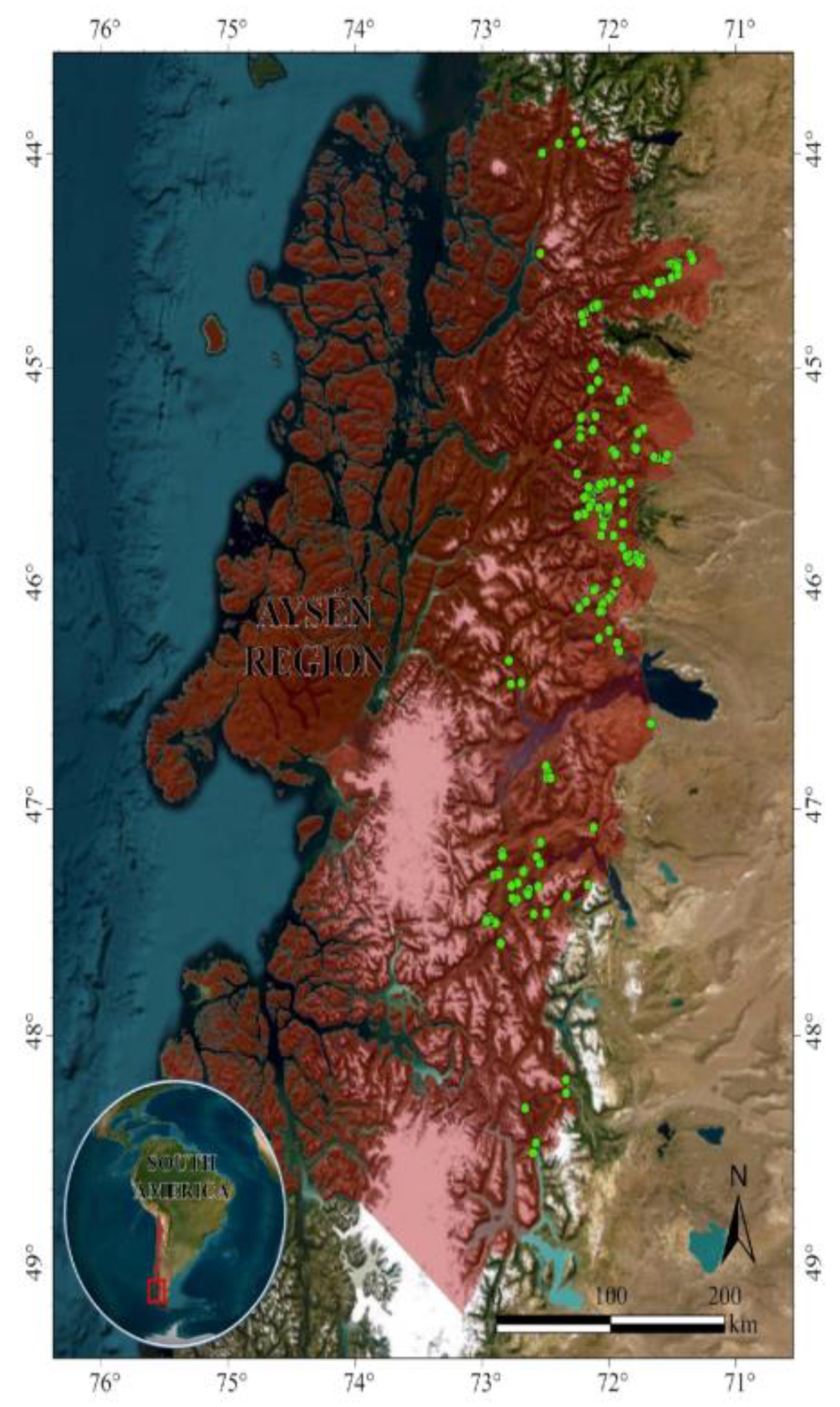
Figure 2.
Data analysis framework for index calculation. (A) Forest treatments based on canopy cover (CC); (B) Plant composition measured by the point-interception method (PIM); (C) Plant nitrogen content measurements to calculate the crude protein (CP); (D) and (E) indices determination based on crude protein index (CPI), phenological index (PHI), plant specific quality (SQ), specific quality index (SQI), pastoral value index (PVI), potential forage production (PFP), and potential animal load (PAL).
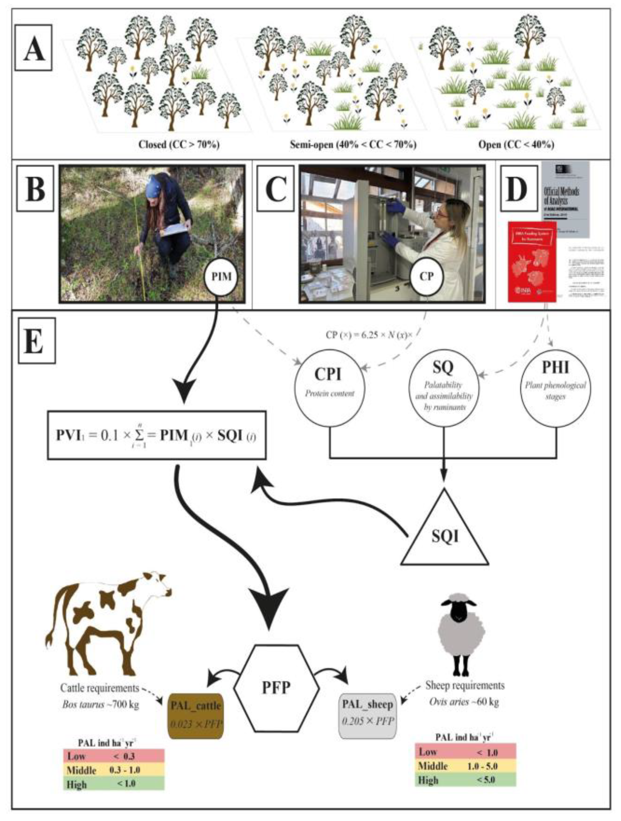
Figure 3.
ANOVAs for potential animal load (PAL) ratio (ind ha-1 yr-1) for sheep and cattle (indicated by sheep and cattle icons) across different seasons and environment types. Different lowercase letters above each bar indicate significant differences between the levels (Tukey test at p <0.05). ÑI = ñire, LE = lenga, CO = coihue, MI = mixed, SV = evergreen, OL = open-lands.

Figure 4.
ANOVA for mean potential animal load (PAL) ratio (ind ha-1 yr-1) for sheep and cattle (indicated by sheep and cattle icons) across different seasons and forest canopy cover (closed, semi-open, open) and open-lands (OL). Different letters above the bars indicate significant differences between the levels (Tukey test at p <0.05).
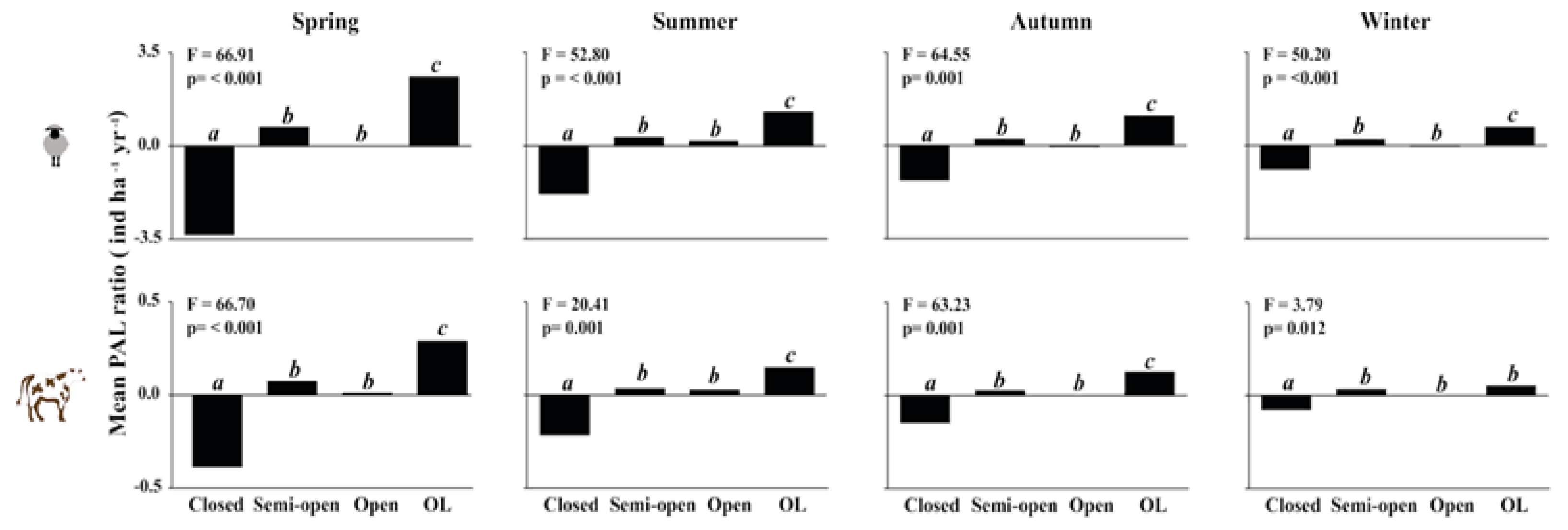
Figure 5.
Multiple Correspondence Analysis showing the relationship between the analyzed environment types (ÑI = ñire, LE = lenga, CO = coihue, MI = mixed, SV = evergreen, OL = open-lands), canopy cover (closed, semi-open, open) and OL, and the potential animal load (PAL, ind ha-1 yr-1) categories: low (red dotted oval), medium (yellow dotted oval), and high (green dotted oval) for sheep (S) and cattle (C). Colored letters represent their PAL data across different seasons (light green for spring, purple for summer, brown for autumn, blue for winter).
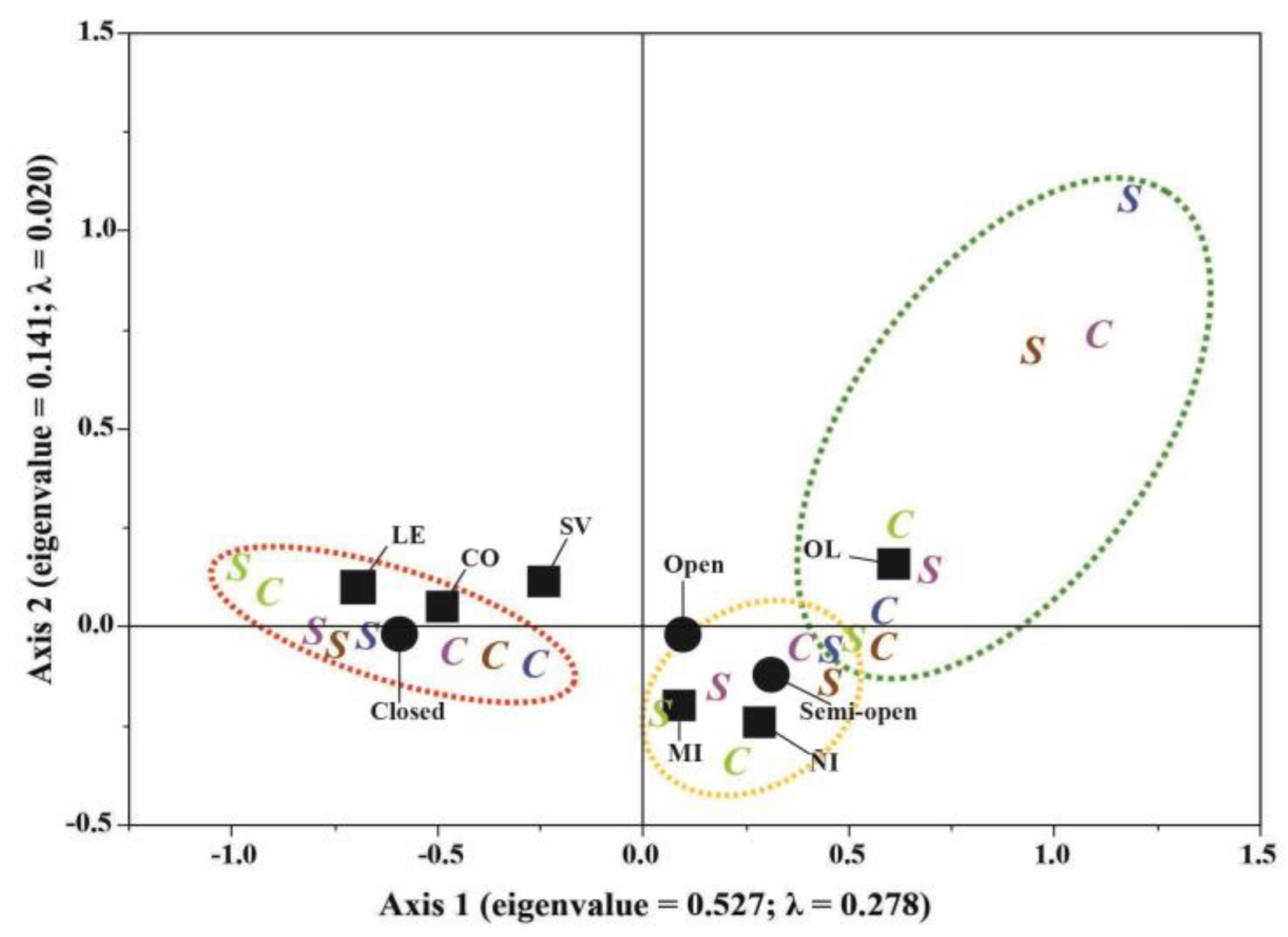
Figure 6.
Multiple Correspondence Analysis showing the relationship between the understory cover (%) of native (light green) and exotic (orange) species across the analyzed environment types and the potential animal load (PAL, ind ha-1 yr-1) categories: low (red dotted oval), medium (yellow dotted oval), and high (green dotted oval) for sheep and cattle. The cattle and sheep symbols represent the centroids for low, medium, and high PAL categories.
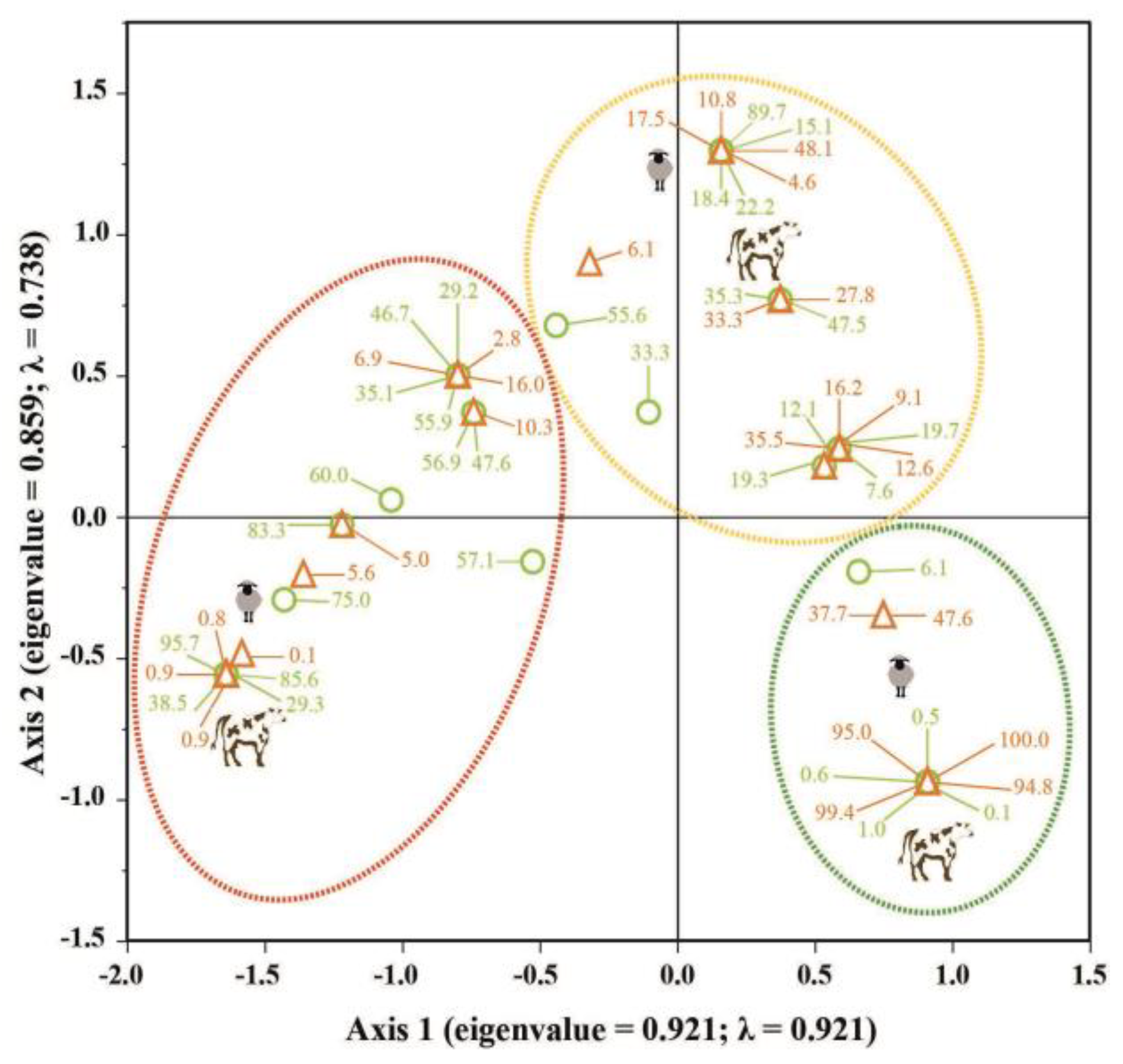
Figure 7.
Example of the season influence on vegetation cover at one plot of the study site.
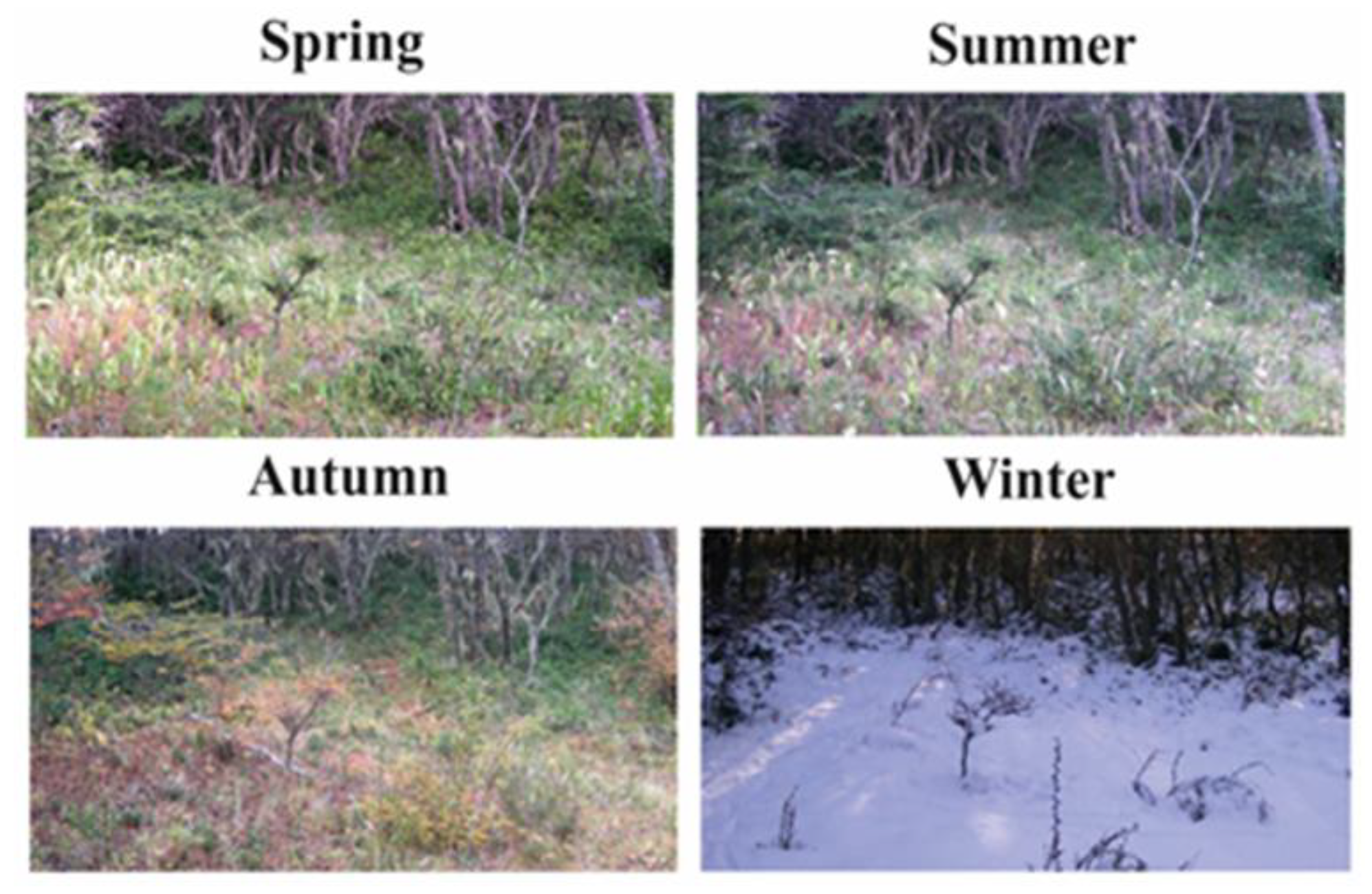
Table 1.
One-way ANOVA results for vegetation cover (%) classified by plant origin and growth habit, including woody debris and bare soil, in different environment types (CO = coihue, LE = lenga, MI = mixed, ÑI = ñire, SV = evergreen, OL = open-lands).
Table 1.
One-way ANOVA results for vegetation cover (%) classified by plant origin and growth habit, including woody debris and bare soil, in different environment types (CO = coihue, LE = lenga, MI = mixed, ÑI = ñire, SV = evergreen, OL = open-lands).
| Variables | ÑI | LE | CO | MI | SV | OL | F(p) |
| Native species | 38.0b | 58.4c | 46.1b | 42.2b | 40.5b | 21.6a | 27.44(<0.01) |
| Exotic species | 53.4b | 16.4a | 22.6a | 34.4ab | 33.2ab | 68.6c | 52.85(<0.01) |
| Trees | 2.7b | 6.7c | 6.3c | 2.1b | 2.8ab | 0.3a | 12.38(<0.01) |
| Shrubs | 15.3c | 12.8b | 13.4b | 11.1ab | 11.5ab | 6.4a | 5.98(<0.01) |
| Forbs | 35.5b | 34.7b | 23.1a | 28.8ab | 28.1ab | 31.9b | 2.83(0.02) |
| Graminoids | 30.1b | 11.9a | 10.7a | 21.5ab | 16.9ab | 44.8c | 37.20(<0.01) |
| Ferns | 5.4 | 3.5 | 6.5 | 7.1 | 5.9 | 3.3 | 2.06(0.07) |
| Lianas | 0.1a | - | 1.0b | - | 1.1b | - | 14.08(0.01) |
| Lichens | 0.4b | 0.8c | 0.1a | - | 0.2b | 0.1a | 3.03(0.01) |
| Bryophytes | 1.9a | 4.4b | 7.6c | 6.0bc | 7.2c | 3.4ab | 5.16(0.01) |
| Total | 91.4b | 74.8a | 68.7a | 76.6a | 73.7a | 90.2a | 29.57(<0.01) |
| Coarse-woody debris | 4.1a | 21.0c | 27.4c | 17.4bc | 14.0b | 3.7a | 34.05(<0.01) |
| Bare soil | 4.5a | 4.2a | 3.9a | 6.0a | 12.3b | 6.1a | 2.80(0.02) |
F = Fisher test, (p) = significance level. Different letters for each row indicate differences by the Tukey tests at p <0.05.
Table 2.
One-way ANOVA results for vegetation cover (%) classified by plant origin and growth habit, including woody debris and bare soil, in different forest canopy cover levels (closed, semi-open, open) and open-lands (OL).
Table 2.
One-way ANOVA results for vegetation cover (%) classified by plant origin and growth habit, including woody debris and bare soil, in different forest canopy cover levels (closed, semi-open, open) and open-lands (OL).
| Variables | Closed | Semi-Open | Open | OL | F(p) |
| Native species | 56.6c | 36.2b | 33.3ab | 21.5a | 51.70(<0.01) |
| Exotic species | 20.4a | 51.9c | 39.6b | 68.6d | 77.84(<0.01) |
| Trees | 6.1c | 2.7b | 1.2a | 0.2a | 18.63(<0.01) |
| Shrubs | 15.1c | 11.8b | 11.8b | 6.2a | 10.45(<0.01) |
| Forbs | 31.4a | 37.0b | 31.0a | 31.1a | 2.73(0.04) |
| Graminoids | 12.6a | 30.1b | 27.6b | 45.8c | 61.33(<0.01) |
| Ferns | 6.1c | 3.3b | 0.3a | 3.3b | 5.77(0.01) |
| Lianas | 0.2 | 0.1 | - | - | 2.17(0.09) |
| Lichens | 0.6 | 0.5 | - | 0.1 | 2.26(0.08) |
| Bryophytes | 4.9c | 2.6b | 1.0a | 3.4b | 3.94(0.01) |
| Total | 77.0a | 88.1b | 72.9a | 90.1b | 22.91(<0.01) |
| Coarse-woody debris | 20.6c | 5.9b | 0.8a | 3.7b | 44.05(<0.01) |
| Bare soil | 2.4a | 6.0b | 26.3c | 6.2b | 40.06(<0.01) |
F = Fisher test, (p) = significance level. Different letters for each row indicate differences by the Tukey tests at p <0.05.
Disclaimer/Publisher’s Note: The statements, opinions and data contained in all publications are solely those of the individual author(s) and contributor(s) and not of MDPI and/or the editor(s). MDPI and/or the editor(s) disclaim responsibility for any injury to people or property resulting from any ideas, methods, instructions or products referred to in the content. |
© 2025 by the authors. Licensee MDPI, Basel, Switzerland. This article is an open access article distributed under the terms and conditions of the Creative Commons Attribution (CC BY) license (http://creativecommons.org/licenses/by/4.0/).
Copyright: This open access article is published under a Creative Commons CC BY 4.0 license, which permit the free download, distribution, and reuse, provided that the author and preprint are cited in any reuse.


