
Submitted:
11 April 2025
Posted:
14 April 2025
You are already at the latest version
Abstract
This article proposes a mathematical model for experimental estimation of the volumetric heat capacity and thermal conductivity of flat samples, in particular samples cut from potato tubers. The method involved using two pairs of samples, each of which includes the test sample and a reference sample. The pairs of samples were pre-cooled in a refrigerator to a temperature that was 10…15°С below room temperature. Then the samples were removed from the refrigerator and placed in an air thermostat at ambient temperature, with one pair of samples additionally blown with a weak air flow. Using a thermal imager, the surface temperatures of the samples were recorded. The temperature measurement results were processed using the proposed mathematical models. The temperature measurement results of the reference samples were used to determine the Bi numbers characterizing the heat exchange conditions on the surfaces of the test samples. Taking into account the found Bi values, the volumetric heat capacity and thermal conductivity were calculated using the formulas described in the article. The article also presents a diagram of the measuring device and a method for processing experimental data using the results of experiments as an example, where potato samples were used as the test samples, and polymethyl methacrylate samples were used as the reference samples. The studies were conducted at an ambient air temperature of 20..24°С and at Bi< 0.3. The volumetric heat capacity of the potato samples was 2.308 MJ/(m³K), and the thermal conductivity was 0.17 W/(m·K).
Keywords:
thermophysical properties
; active thermography
; modeling of temperature fields
1. Introduction
Potatoes are important food products in many countries of the world. At various stages of their life cycle, in particular, during storage and treatment, it is necessary to maintain specified temperature conditions, since they affect the shelf life or quality of the resulting food products. Information about the temperature field in potatoes is necessary to control the processes of drying [1], blanching [2], frying [3], when determining the optimal storage parameters [4] or thermal control [5], ensuring the detection of various defects, such as rot.
To describe temperature fields of potato tubers in three-dimensional space of Cartesian coordinates x, y, z, in the general case, equations of the form are used with the corresponding boundary and initial conditions, where a is the thermal diffusivity coefficient of potato plant tissue, defined as the ratio of its thermal conductivity λ and volumetric heat capacity сv. Thermal conductivity and volumetric heat capacity are important thermophysical properties of the material, determining, among other things, the rate of change of its temperature field. For potatoes, they significantly depend on its moisture content, density, and also the qualitative state of the plant tissue. For example, the internal structure is determined by the presence of defects, as well as other parameters. Therefore, information on the thermophysical properties of potato plant tissues, used to model temperature fields and obtained for potatoes of one variety, cannot be used for potatoes of another variety, or growing in another area. From this point of view, for mass measurements, a comparatively simple and cheap method of experimental estimation of thermophysical properties of potatoes is needed.
In relation to food products, many methods for determining thermophysical properties have been developed over the past few decades. In this case, one can distinguish between stationary and non-stationary measurement methods [6], which provide for the thermal effect on the test object from sources of various physical natures - microwave radiation [7], laser [8], and others.
Stationary methods involve measuring thermophysical properties under conditions of a steady-state temperature field of the test object. In particular, the classical approach is to apply a constant heat flow to one of the surfaces of the test sample, for example, a flat surface [9,10]. The experiment measures the steady-state temperature difference across the thickness of the sample, which is inversely proportional, according to Fourier’s law, to thermal conductivity. The advantage of stationary methods is their simplicity and high accuracy in determining thermal conductivity. At the same time, the experiment is characterized by a long duration.
In terms of increasing the speed of the experiment, non-stationary methods are more advantageous. In addition, such methods often provide information about several thermophysical properties, such as thermal conductivity and thermal diffusivity, in a single experiment. Non-stationary methods involve the impact of a heat flow of constant or variable power on the control object and the recording of a non-stationary temperature field in the object as a response to such an impact. In relation to the study of the thermophysical properties of plant tissues, we can highlight several works devoted to the development of non-stationary methods. Thus, the authors of [11] proposed to briefly expose the leaves of spring barley (Hordeum vulgare) and common beans (Phaseolus vulgaris) to a heat pulse and measure the parameters of the leaf cooling process to determine its heat capacity under various heat exchange conditions on the surface. In [12], it is shown that when a plant is exposed to a pulse lasting up to 10 s and the temperature response is subsequently measured, it is possible to determine the volumetric heat capacity by fitting a leaf energy balance model to a leaf temperature transient. In contrast to [11,12], where a LED lamp was used as a source of thermal impulse, the authors of [8] used a laser to affect the surface of the leaf, recorded the thermal response using thermal imaging equipment and determined the thermal conductivity and heat capacity. A fairly simple method for measuring the thermal diffusivity of various plant foods was considered in [13]. Its authors gave samples of potatoes, carrots and a number of other products a spherical shape. They placed a thermocouple in the center of the sample and placed the resulting sample-thermocouple system in boiling water. Thermocouple readings were recorded. Since a constant temperature equal to the boiling point of water was maintained on the surface of the sample, regularization of the temperature field was observed in the sample after some time of the experiment, which was expressed in a constant rate of its change. Solving the problem of heat transfer in a spherical body with boundary conditions in the form of a constant temperature, the authors of [13] obtained a simple expression for determining the thermal diffusivity. However, in our opinion, this approach has its drawbacks. In particular, it is quite difficult to give plant tissue samples the correct spherical shape, and it is also difficult to place the working junction of the thermocouple exactly in the center of the sample. In addition, the effect of high temperature on a plant tissue sample leads to a change in its physical properties. In particular, when potatoes are heat treated, the starch contained in them is gelatinized. Protopectin, which binds plant cells together, is converted into pectin during heat treatment, which is accompanied by softening of the plant tissue. The cellulose contained in the plant tissue swells and becomes more porous.
The review showed that there are methods for obtaining experimental information about the thermophysical properties of plant tissues. It is also shown that the methods that we could use to study the thermophysical properties of potatoes provide either heating of a local area of the test object, or the entire object, as shown in [13], to temperatures that lead to the destruction of plant tissue, which can lead to a change in its thermophysical properties. Therefore, in this study, we set the goal of modifying the known methods and creating a simple and inexpensive method for measuring thermophysical properties on their basis. The implementation of the method should not provide for a strong thermal effect on the test object, leading to the destruction of its plant tissue in the experiment.
2. Materials and Methods
2.1. Sample Preparation and Experiment
For the experimental study of thermophysical properties, we cut out two samples 1, 2 of the same thickness h<D/10 from a whole potato tuber with a transverse diameter D of at least 50 mm. The thickness of the samples usually ranged from 3 to 3.5 mm (Figure 1a). Apart from the test samples of potatoes, we used two identical samples 1’ and 2’ with the known values of thermal conductivity λ’ and thermal diffusivity а’. Hereinafter, samples 1’ and 2’ will be called reference samples. These samples are disks with a diameter D and a thickness h’≈h, made of polymethyl methacrylate. The test samples 1, 2 and the reference samples 1’, 2’ were cooled in a refrigerator to a temperature of T0 = 10..150С for 1.5…2 hours. Then pairs of samples 1, 1’ and 2, 2’ were quickly placed in heat chambers 3 and 4, respectively (Figure 1b). A constant temperature equal to the ambient air temperature Tair was maintained in the thermal chambers, with Tair> T0 by 10…120C. In thermal chamber 4, samples 2, 2’ were additionally blown with an air flow from fan 5, similar to those used for cooling in computers. During the experiment, a Flir A35 thermal imager 6 was used to record the change in surface temperature over time for each of the samples, which were heated from the initial temperature T0 to the temperature Tair. Moreover, to minimize the influence of edge effects on the temperature measurement results, we measured temperatures in a circular area with a diameter of d=10 mm on the surface of each of the samples (Figure 1a).
2.2. Mathematical Models of Heat Transfer in Test and Reference Samples
We write the mathematical model of the temperature field T(x, τ) for half of a flat sample (0≤x≤h/2) (Figure 2), since it is symmetrical with respect to the coordinate x=0 if the condition h<D/10 is met. Boundary conditions are specified at the outer boundaries of the plate – heat exchange with the surrounding air at temperature Tair and at a constant heat transfer coefficient α. At the initial moment of time, at τ=0, the temperature inside the sample is equal to T0.
Denoting Θ=[T(x, τ)- T0]/[ Tair- T0], we write the expression for the dimensionless temperature on the plate surface [14]: Θ=1-), where .
Here Bi=αr/λ is the Biot number; r is half the thickness of the sample; λ is the thermal conductivity of the sample; Fo=aτ/r2 is the Fourier number; а is the thermal diffusivity of the sample; is the root of the characteristic equation ctg=.
Let us consider a special case when Bi<0.3. In practice, it is realized when the sample surface is not blown or is blown by a weak air flow. In this case, А1≈1, А2 and subsequent terms tend to zero. In this case, also, for small values of tg can be replaced with . Then the above characteristic equation will take the form . Taking this into account, we write expressions for dimensionless temperatures on the surfaces of the studied and reference samples:
where i is the sample number, i=1,2, 1’, 2’.
To calculate the Biot Bi and Fourier Fo criteria, the following expressions are used: Bii=αiri/λi; Foi=aiτ/r2, where r= h/2 at i=1,2 and r= h’/2 at i =1’, 2’.
Also, taking into account the equality of the thermophysical properties of samples 1,2, as well as samples 1’, 2’, we introduce the designations: λ1=λ2= λ; a1= a2= a; λ1’=λ2’= λ’ and a1’= a2’= a’.
Since the thermophysical properties of the reference samples are known to us, then in equation (1), written for i =1’, 2’ for the reference samples, the only unknown parameters are the Biot numbers: Bi1’= 0.5α1’h’/λ’ и Bi2’= 0.5α2’h’/λ’. To determine them, we used the following method.
Setting Bi1’ and Bi2’ in the range 0<Bi≤0.3 from (1) determines the calculated temperature Ti(h’/2, τ) on the surface of each reference sample. Next, we determine the values of the deviation Err of the calculated data from the experimental Tiexp(h’/2, τ), using the expression
It should be noted that to find Bi1’ we can use the previously given expression . Taking this expression into account, we write equation (1) for i=1’ as
1-Θ1’=1-[ T1’(h’/2, τ) - T0]/[ Tair- T0]=cos exp(- Fo1’). Taking the logarithm of the last expression, we obtain
From the obtained expression it is clear that the desired number Bi can be defined as the tangent of the slope of the linear function ln(1-Θ)=f( Fo).
By similarly determining Bi2’, we can calculate the values of the heat transfer coefficients α1’= 2Bi1’λ’/h’ and α2’= 2Bi2’λ’/h’. Making the assumption that the heat transfer coefficients on the surfaces of the test and reference samples are equal, i.e. α1’ =α1 and α2’=α2, it is possible to determine Bi1= 0.5α1h/λ and Bi2= 0.5α2h/λ. It should be recognized that such an assumption requires some justification and imposes restrictions on the experimental conditions. In particular, moisture evaporation can be observed from the surface of the test potato sample, which leads to an increase in the heat exchange intensity. In this case, α1> α1’. However, at relatively high air humidity and at Tair> T0 by 10...12 0С moisture evaporation will be insignificant. In addition, to reduce the evaporation effect and ensure the same surface roughness of the test and reference samples, we recommend covering them with a thin polyethylene film up to 30 μm thick. In this case, the effect of the thermal resistance of the film layer on the surface temperature of the samples can be neglected.
With known values of heat transfer coefficients α1, α2 in equations (1) at i=1,2, the unknown parameters are the thermophysical properties λ and a of the test samples. We write expression (3) at i=1 as ln(1-Θ1)=Const-/(rcv)τ. In the resulting expression, we denote B1= /(rcv). From the last expression, we can determine the volumetric heat capacity of the test sample:
cv = 2α1/(B1h).
The introduced parameter B1 is found experimentally as the tangent of the slope of the rectilinear section of the function ln(1-Θ1)=f(τ).
To determine the thermal conductivity λ of the test sample from the boundary conditions at x=r, which have the form - λ∂Ti(x=r,τ)/∂x+ αi[Tair- Ti(x=r,τ)]=0, taking into account (1), we obtain the expression
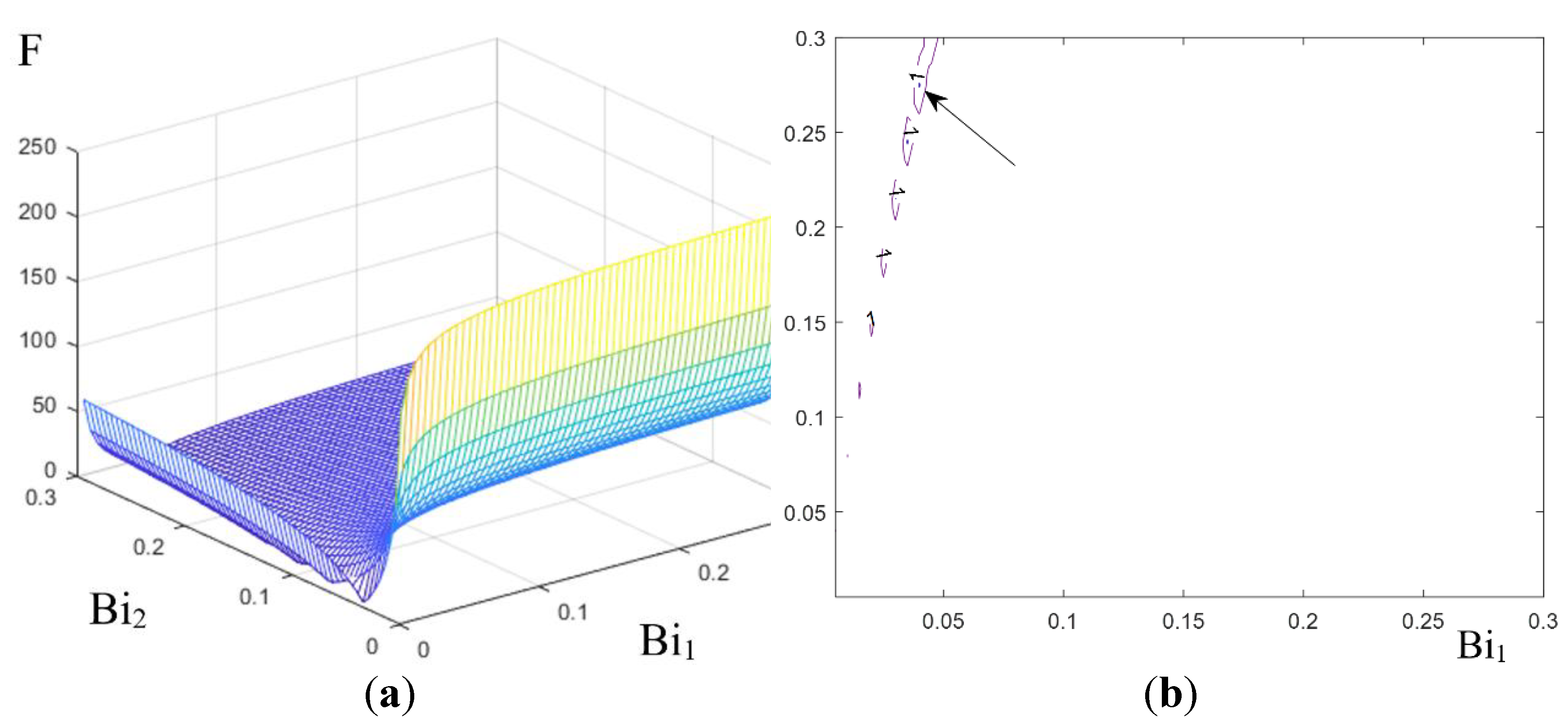
α1 cos1/ sin1= α2 cos2/ sin2 or α1 ctg1= α2 ctg2. Let F denote the function:
We find the minimum Fmin of the function F and the corresponding pairs of values Bi1,Bi2. Then the desired thermal conductivity of the test material can be found from the expression
λ = 0.25h (α1/ Bi1 + α2/ Bi2).
3. Results
Let us consider the algorithm for determining the thermophysical properties of potatoes using a specific example. In the example, the reference samples 1’ and 2’ made of polymethyl methacrylate had a thickness of h’=4.5 mm, their thermophysical properties are λ’=0.195 W/(m·K) and a’=1,29·10-7 m2/s. Samples 1, 2, cut from potatoes, were used as the test samples. The thickness of the samples was h=3.5 mm. The temperature curves T1’exp,T2’exp, T1exp, T2exp, were found, and are shown in Figure 3. The experiments were carried out at Tair=20.5 0С for samples 1, 1’ and at Tair=24.5 0С for samples 2, 2’. In the presented example, the potato samples were not covered with polyethylene film on top. Since the cut was fresh and wet, the temperature of the potato in the experiments with τ tending to infinity was 2...3 0С lower than the temperature of the standard.
Setting Bi1’ and Bi2’ in the range 0<Bi≤0.3 using formulas (1), the calculated temperature Ti(h’/2, τ) on the surface of each reference sample was determined. Using (2), we calculated Erri, as the sum of the squares of the deviations of the calculated temperature from the experimental one. As an example, Figure 4 shows a dependence graph of Err1’ on Bi1’. As can be seen from the example shown in Figure 4, the dependence graph Err(Bi) has a minimum at Bi1’=0.07.
Figure 5 shows the second method for finding the desired parameter Bi. The figure demonstrates that the desired number Bi can be defined as the tangent of the slope of the linear function ln(1-Θ) = f(Fo).
Bi2’=0.23was determined in a similar way, after which the values of the heat transfer coefficients α1’= 6,1 and α2’=19,9 W/(m2K) were calculated.
The results of measuring the temperature of sample 1 (curve 1 in Figure 3) were used to calculate the parameter B2 = 0.0015, as the tangent of the slope of rectilinear section of the dependency ln(1-Θ1) = f(τ) (Figure 6). Then, using (4), (4), cv=2.308 MJ /(m3·K) was found.
When determining the thermal conductivity, we found the coordinates Bi1 and Bi2 of the minimum point of function (5). In Figure 7b, the arrow shows the value Fmin=0.1 for the function shown in Figure 7a. The values of the Biot numbers corresponding to this minimum are Bi1=0.05 and Bi2=0.27. Note that, depending on the accuracy of the calculations, the minimum of the function F can be observed in the vicinity of several points with coordinates Bi1, Bi2. For example, in Figure 7b, at Fmin=1, several minimum regions are observed, which significantly increases the uncertainty of measuring λ. As a result of calculating the thermal conductivity according to (6), we obtained the following value λ=0,17 W/(m·K).
It should be noted that with an average potato density of 1110 kg/m3, taking into account the obtained value cv=2.308 MJ/(m3K), the specific heat capacity of potatoes is 2.5 kJ/(kg·K), which is in good agreement with the known data from literary sources [15]. At the same time, the result of measuring thermal conductivity contains significant uncertainty and varies in the range from 0.17 to 0.3 W/(m·K), while literary sources provide a range from 0.2 to 0.5 W/(m·K). We explain this difference by the fact that thermal conductivity significantly depends on the moisture content of the samples, the variety and places of growth, as well as weather conditions and storage conditions of potatoes.
4. Conclusions
Information on thermophysical properties, in particular on thermal conductivity, heat capacity, thermal diffusivity of plant tissues of fruits and vegetables is required when solving problems of heat transfer modeling under conditions of transportation, storage, preparation of various dishes. Despite the existing fairly extensive knowledge base on the thermophysical properties of fruit and vegetable products, simple, cheap methods for experimental determination of thermophysical properties are required. This is explained by the fact that the thermophysical properties of the objects of control significantly depend on the variety, growing places, growing and storage conditions. Therefore, the thermal conductivity or thermal diffusivity of fruits or vegetables of the same variety, but grown in different fields or gardens, can differ significantly. In this article, we demonstrated the possibility of determining a set of thermophysical properties of potatoes - volumetric heat capacity and thermal conductivity by conducting two experiments with flat test samples that were pre-cooled and then heated at room temperature under conditions of natural convection on their surface or with a weak blower. In this case, the heat exchange conditions were characterized by the number Bi<0.3, determined from the experiment with flat reference samples, the thermophysical properties of which were known. This approach allowed the use of simple calculation formulas for calculating the thermophysical properties of the materials under study. At the same time, it was shown that the results of determining thermal conductivity may contain significant uncertainties. Therefore, the proposed method cannot be considered as a precision method for measuring thermophysical properties. For its further development, it is necessary to study the metrological characteristics, determine the optimal conditions for conducting experiments, under which the uncertainties in measuring thermophysical properties will be minimal. This is planned to be done in subsequent studies. It should also be noted that the method can be used not only to study the thermophysical properties of flat potato samples, but also other materials of plant origin, which can be given the appropriate shape, including apples and pears.
Author Contributions
P.B.: conceptualization, data curation, writing—original draft preparation, supervision; A.E.: funding acquisition, validation, software; A.D.: formal analysis, investigation, visualization. All authors have read and agreed to the published version of the manuscript.
Funding
This research was funded by financial support from the Ministry of Science and Higher Education of the Russian Federation within the framework of the project “Development of a robotic complex of ground and air unmanned platforms for use in agricultural technologies” (124062100023-3).
Data Availability Statement
Data are contained within the article.
Conflicts of Interest
The authors declare no conflicts of interest.
References
- Heshmati, M. K.; Khiavi, H. D.; Dehghanny, J.; Baghban, H. 3D simulation of momentum, heat and mass transfer in potato cubes during intermittent microwave-convective hot air drying. Heat Mass Transf. Und Stoffuebertragung 2023, 59, 345–363. [Google Scholar] [CrossRef]
- Lamberg, I.; Hallström, B. Thermal properties of potatoes and a computer simulation of a blanching process. Int. J. Food Sci. Technol. 2007, 21, 577–585. [Google Scholar] [CrossRef]
- Costa, R. M.; Oliveira, F. A.; Delaney, O.; Gekas, V. Analysis of the heat transfer coefficient during potato frying. J. Food Eng. 1999, 39, 293–299. [Google Scholar] [CrossRef]
- Öztürk, E.; Taşkın, P. The effect of long term storage on physical and chemical properties of potato. Turk. J. Field Crops 2016, 21, 218–223. [Google Scholar] [CrossRef]
- Balabanov, P.; Egorov, A.; Divin, A.; Ponomarev, S.; et al. Mathematical Modeling of the Heat Transfer Process in Spherical Objects with Flat, Cylindrical and Spherical Defects. Computation 2024, 12, 148. [Google Scholar] [CrossRef]
- Yüksel, N. The Review of Some Commonly Used Methods and Techniques to Measure the Thermal Conductivity of Insulation Materials; Insulation Materials in Context of Sustainability, 2016; pp. 113–140. [Google Scholar] [CrossRef]
- Giedd, R.; Giedd, G. Thermal Conduction Measurements of Materials using Microwave Energy. MRS Proc. 1990, 189, 55–60. [Google Scholar] [CrossRef]
- Buyel, J.F.; Gruchow, H.M.; Tödter, N.; Wehner, M. Determination of the thermal properties of leaves by non-invasive contact-free laser probing. J. Biotechnol. 2016, 217, 100–108. [Google Scholar] [CrossRef] [PubMed]
- Jannot, Y.; Remy, B.; Degiovanni, A. Measurement of thermal conductivity and thermal resistance with a tiny hot plate. High Temp. -High Press. 2010, 39, 11–31. [Google Scholar]
- Matteis, P.; Campagnoli, E.; Firrao, D.; Ruscica, G. Thermal diffusivity measurements of metastable austenite during continuous cooling. Int. J. Therm. Sci. 2008, 47, 695–708. [Google Scholar] [CrossRef]
- Albrecht, H.; Fiorani, F.; Pieruschka, R.; Müller-Linow, M.; et al. Quantitative Estimation of Leaf Heat Transfer Coefficients by Active Thermography at Varying Boundary Layer Conditions. Front. Plant Sci. 2020, 10, 1684. [Google Scholar] [CrossRef] [PubMed]
- Zhang, J.; Kaiser, E.; Zhang, H.; et al. A simple new method to determine leaf specific heat capacity. Plant Methods 2025, 21, 1–13. [Google Scholar] [CrossRef] [PubMed]
- Wang, L.; Jin, Y.; Wang, J. A simple and low-cost experimental method to determine the thermal diffusivity of various types of foods. Am. J. Phys. 2022, 90, 568–572. [Google Scholar] [CrossRef]
- Lykov, A.V. Teoriya teploprovodnosti [Theory of thermal conductivity]; (in Russ.); Vysshaya shkola: Moscow, 1967. [Google Scholar]
- Farinu, A.; Baik, O.-D. Thermal Properties of Sweet Potato with its Moisture Content and Temperature. Int. J. Food Prop. 2007, 10, 703–719. [Google Scholar] [CrossRef]
Figure 1.
(a) Test samples; (b) Measuring setup.
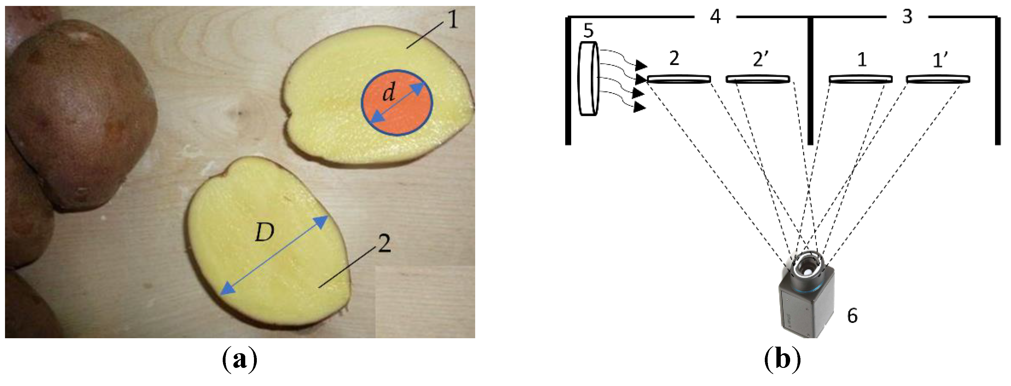
Figure 2.
Physical model of flat sample.
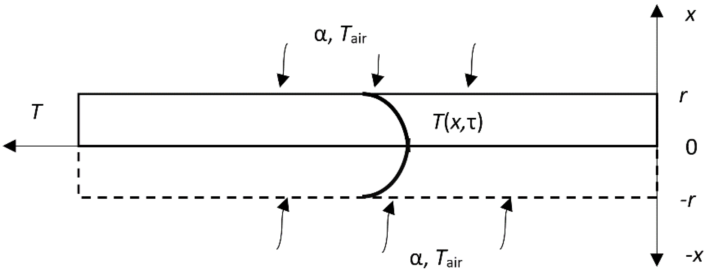
Figure 3.
Dependency graphs of experimental temperature over time for reference 1’, 2’ and test 1,2 samples.
Figure 3.
Dependency graphs of experimental temperature over time for reference 1’, 2’ and test 1,2 samples.
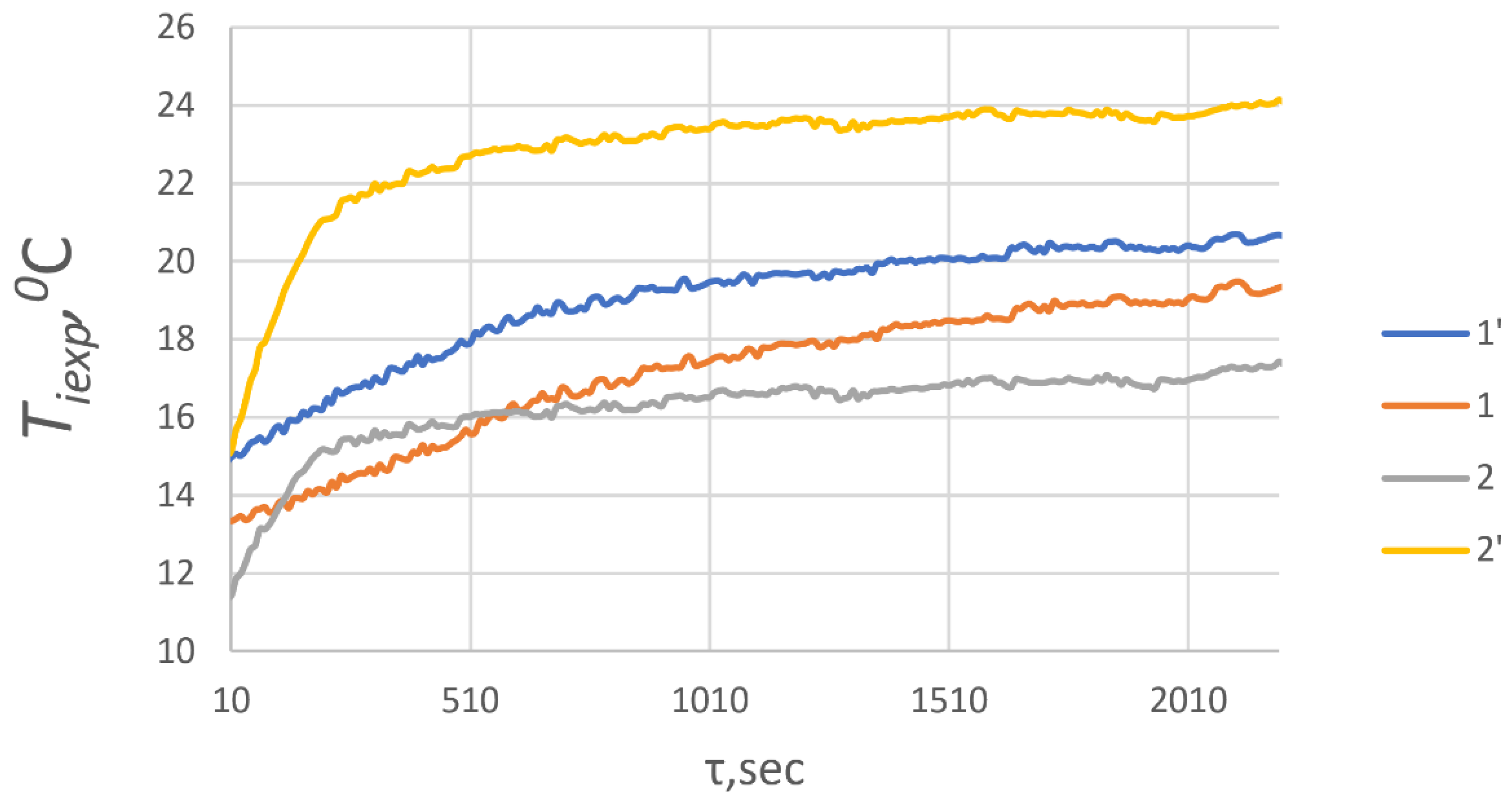
Figure 4.
Graphs of deviation Err versus Bi for sample 1’.
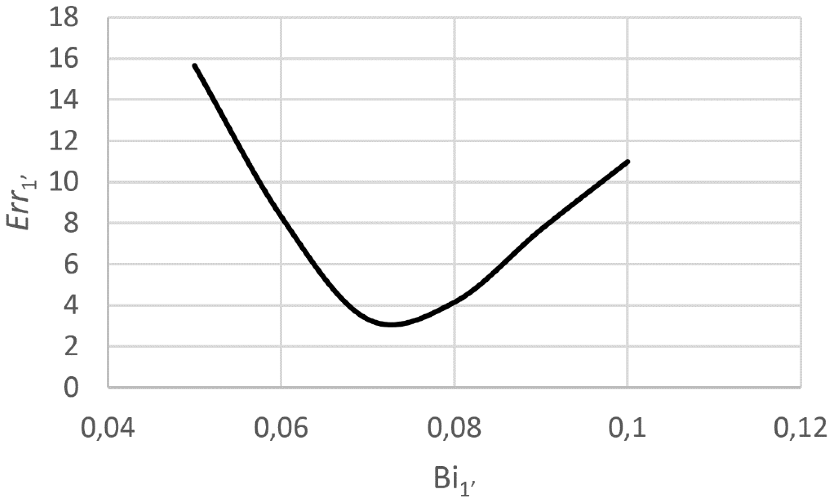
Figure 5.
Dependency graph ln(1-Θ1’) = f(Fo1’).
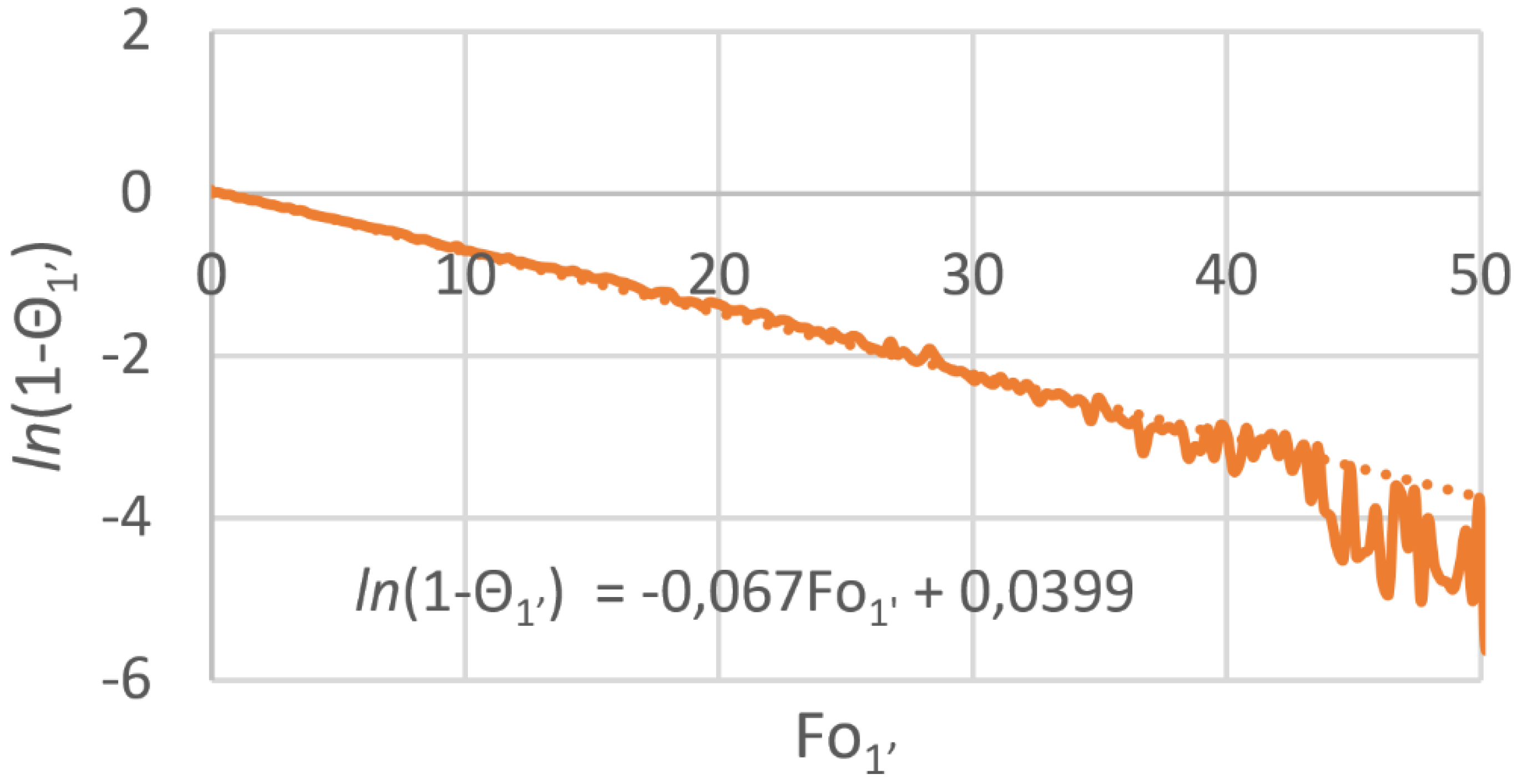
Figure 6.
Dependency graph ln(1-Θ1) = f(τ).
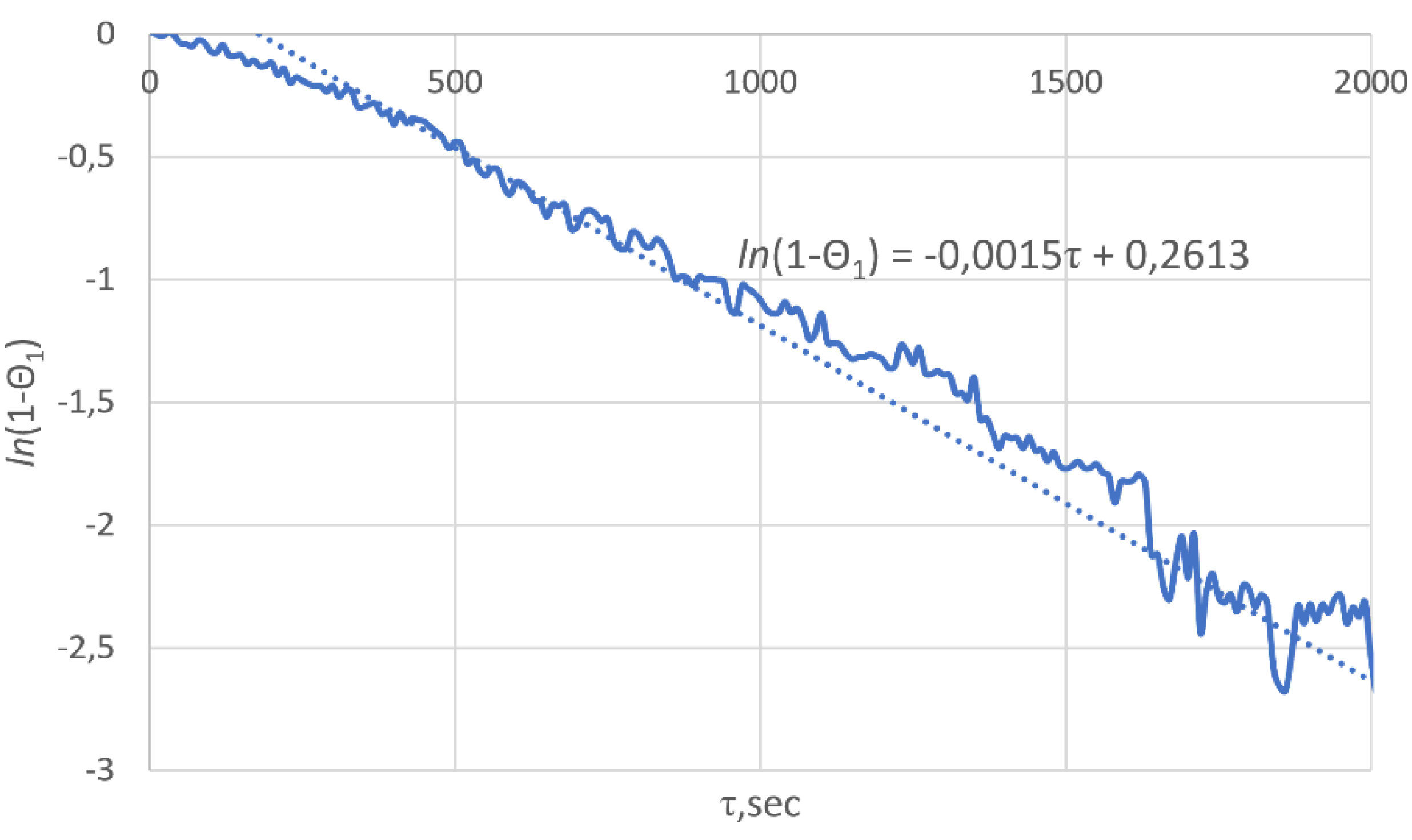
Figure 7.
Dependency graphs at α1=6,1 and α2=19,9 W/(m2K): (a) F(Bi1, Bi2); (b) F(Bi1, Bi2) = 1.
Disclaimer/Publisher’s Note: The statements, opinions and data contained in all publications are solely those of the individual author(s) and contributor(s) and not of MDPI and/or the editor(s). MDPI and/or the editor(s) disclaim responsibility for any injury to people or property resulting from any ideas, methods, instructions or products referred to in the content. |
© 2025 by the authors. Licensee MDPI, Basel, Switzerland. This article is an open access article distributed under the terms and conditions of the Creative Commons Attribution (CC BY) license (http://creativecommons.org/licenses/by/4.0/).
Copyright: This open access article is published under a Creative Commons CC BY 4.0 license, which permit the free download, distribution, and reuse, provided that the author and preprint are cited in any reuse.


