Research on AI Economic Cycle Prediction Method Based on Big Data

1. Introduction

With the rapid development of big data technology, the timeliness, breadth and depth of economic data have been dramatically improved, providing new ideas for economic cycle prediction based on artificial intelligence (AI) [1]. With powerful nonlinear modeling capabilities, deep learning methods can effectively extract the time-series characteristics of economic variables and improve the prediction accuracy. How to construct an efficient AI prediction framework, optimize the key algorithms and improve the generalization ability of the model remains the core issue of current research.

2. Big Data-Driven Characterization of Economic Cycles

2.1. Multidimensional Big Data Indicator Construction

Accurate prediction of economic cycles relies on multi-dimensional and multi-level data support, so it is necessary to construct a multi-dimensional big data indicator system covering macroeconomic, industrial structure, market behavior and financial variables. At the macroeconomic level, key economic variables such as GDP growth rate, CPI, PPI, unemployment rate, industrial value-added, total retail sales of consumer goods, etc. are selected; at the industrial structure dimension, indicators such as fixed-asset investment, PMI of the manufacturing industry, growth rate of real estate investment, and capacity utilization rate of each industry are introduced; at the market behavior, market volatility indicators such as the volatility of the stock market, bond yields, and credit spreads of enterprises are considered; at the financial variables, a system of multi-dimensional big data indicators is needed to cover the macroeconomic and financial variables. liquidity indicators; in terms of financial variables, focus on the M2 growth rate, short-term interest rates, money multiplier and other monetary policy-related factors [2]. In order to ensure the rationality and consistency of the data, all the indicators are normalized and the standardized formula is defined as follows:

$$X_i^{*}={\displaystyle \frac{X_i-{\mu }_i}{{\sigma }_i}}$$

where $X_i^{*}$ is the normalized variable, $X_i$ is the original data, ${\mu }_i$ and ${\sigma }_i$ and denote the mean and standard deviation of the variable, respectively. In order to eliminate the scale difference between different data sources, min-max normalization method was used for data transformation:

$$X_i^{\prime }={\displaystyle \frac{X_i-\min \left(X_i\right)}{\max \left(X_i\right)-\min \left(X_i\right)}}$$

Through the construction and standardization of the above multi-dimensional data indicators, it can ensure that the data input of the economic cycle prediction model has good stability and comparability, laying a solid foundation for the subsequent feature extraction and model training.

2.2. Data Preprocessing and Feature Engineering

High-quality data preprocessing is a key part of constructing accurate economic cycle prediction models [3]. The original data are processed for missing values, and linear interpolation is used to fill in the small range of missing values, while K-nearest neighbor filling (KNN) or Lagrange interpolation is used for larger missing intervals to ensure the continuity and completeness of the data. Outliers are detected using the Z-score method with the following formula:

$$Z_i={\displaystyle \frac{X_i-\mu }{\sigma }}$$

When $\left|Z_i\right|>3$ is used, it is judged as an outlier and corrected using IQR (interquartile range) or Winsorization methods. In terms of data dimensionality reduction, principal component analysis (PCA) method is utilized to reduce redundant information and improve data interpretability. Let the original data matrix be X and its covariance matrix be Σ, then the principal components are calculated as follows:

$$X^{\prime }=XW$$

where W is the dimensionally reduced transformation matrix composed of the covariance matrix eigenvectors, and only the principal components with a cumulative variance contribution of more than 95% are retained. To enhance the time-series characteristics of the data, lagged variables and sliding window features are constructed so that the dynamic changes of the economic cycle can be fully expressed. Specifically, for the time series data $x_t$, the lagged features are defined as:

$$X_t^{\left(lag\right)}=x_{t-k}$$

where k is the lag order, the optimal lag is usually determined based on ACF (autocorrelation function) and PACF (partial autocorrelation function). Through the above preprocessing and feature engineering, the data quality can be effectively improved, key features in the economic cycle can be mined, and accurate and stable input data can be provided for the AI intelligent forecasting model.

2.3. Identification of Key Features of the Economic Cycle

In economic cycle prediction, the extraction of key features directly determines the prediction accuracy of the model. The essence of the economic cycle is the fluctuation of macroeconomic variables in the time dimension, and feature identification needs to be analyzed in depth by combining time series features, frequency domain features and structural features [4]. Using Empirical Mode Decomposition (EMD) to multi-scale decomposition of economic data, the original time series $X_t$ is decomposed into a number of intrinsic mode functions (IMFs), namely:

$$X_t={\displaystyle \sum _{i=1}^n{IMF}_i}+R_n$$

where ${IMF}_i$ represents the components of economic fluctuations in different time scales, and $R_n$ is the residual term. EMD can effectively separate the short-period high-frequency perturbations from the long-term trend term, providing fine-grained information for economic cycle analysis. Wavelet Transform (WT) is used for frequency domain analysis, and the signal is decomposed with multi-resolution by the scale function ϕ(t) and wavelet function ψ(t):

$$X_t={\displaystyle \sum _j{\displaystyle \sum _k{c}_{j,k}{\psi }_{j,k}}}\left(t\right)$$

where $c_{j,k}$ is the wavelet coefficients, j represents the scale, and k represents the time position. The wavelet transform can effectively extract the cyclical features of economic data and identify the cyclical fluctuation patterns in different time scales. In order to identify the structural inflection point of the economic cycle, Markov Hidden State Model (Markov Switching Model, MSM) is introduced, and the economic state $S_t$ is set to obey the first-order Markov process, and its transfer probability matrix is:

$$P=\left[\begin{array}{cc}{p}_{11}& p_{12}\\ p_{21}& p_{22}\end{array}\right]$$

where $p_{ij}$ denotes the probability of transferring from state i to state j. This method can effectively identify the stage characteristics of economic recession, recovery, and expansion, and improve the sensitivity of the prediction model to the turning point of the cycle. Combining the above methods, the accurate identification of key features of the economic cycle is achieved through multi-scale signal decomposition, frequency domain analysis and hidden state modeling, providing high-quality inputs for the construction of the subsequent AI prediction model.

3. AI Intelligent Prediction Model Construction

3.1. Deep Learning Prediction Framework Design

In economic cycle prediction, the deep learning framework needs to comprehensively consider the time-series characteristics, nonlinear relationship and long-term dependence of data [5]. In this paper, we construct a deep learning prediction framework composed of four core modules: data preprocessing, feature extraction, model training, and prediction output. In the data preprocessing module, multi-dimensional economic indicators are normalized, filled with missing values and time series reconstructed to ensure data consistency and validity. In the feature extraction stage, Long Short-Term Memory (LSTM) and Attention Mechanism are combined to capture the long-term dependencies of economic data through gating units and assign higher weights to key features to improve prediction accuracy [6]. The model training adopts an autoregressive structure, which maps the time series data $X=\left\{x_1,x_2,\dots ,x_{t-n};\theta \right\}$ to the predicted values of the future time step ${\widehat{x}}_{t+1}$:

$${\widehat{x}}_{t+1}=f\left(x_t,x_{t-1},\dots ,x_{t-n};\theta \right)$$

where θ is a model parameter, which is optimized by gradient descent method. The two-layer Bi-LSTM structure is used to enhance the bidirectional propagation ability of the information flow, and combined with the Transformer encoder to further optimize the temporal feature expression. The prediction output module utilizes the regression layer to calculate the future economic indicators and adjusts the model parameters through error analysis to reduce the prediction bias.

3.2. Optimization of Neural Network Algorithm

Economic cycle prediction involves complex nonlinear dynamic features, so the optimization of neural network algorithms is crucial. In this paper, we focus on four aspects: network structure improvement, loss function optimization, regularization strategy and optimization algorithm, in order to enhance the model’s generalization ability and prediction accuracy [7]. In terms of network structure, Bi-LSTM (Bi-LSTM) is introduced to capture the bidirectional dependence of the time series and combined with Attention Mechanism (AM) to enhance the weight allocation of key features.The forward and backward propagation of Bi-LSTM is calculated as follows:

$$\overrightarrow{h_t}=\sigma \left(W_x{x}_t+W_h\overrightarrow{h_{t-1}}+b\right)$$

$$\overleftarrow{h_t}=\sigma \left(W_x{x}_t+W_h\overleftarrow{h_{t-1}}+b\right)$$

The final hidden state $h_t$ is represented by splicing forward and backward states:

$$h_t=⌊\overrightarrow{h_t},\overleftarrow{h_t}⌋$$

For loss function optimization, the Huber loss function (Huber Loss) is used to balance the mean square error (MSE) and mean absolute error (MAE) to avoid outliers affecting the model training:

$$L_{\delta }\left(a\right)=\left\{\begin{array}{l}{\displaystyle \frac{1}{2}}{a}^2,\hspace{1em}\hspace{1em}\hspace{1em}\hspace{0.33em}\hspace{0.33em}if\left|a\right|\le \delta \\ \delta \left(\left|a\right|-{\displaystyle \frac{1}{2}}\delta \right),\hspace{1em}if\left|a\right|>\delta \end{array}\right.$$

where $a=y-\widehat{y}$ denotes the difference between the true value and the predicted value, and δ is a hyperparameter. To prevent overfitting, L2 regularization (weight decay) with Dropout mechanism is introduced and AdamW optimization algorithm is used to enhance training stability and convergence speed.

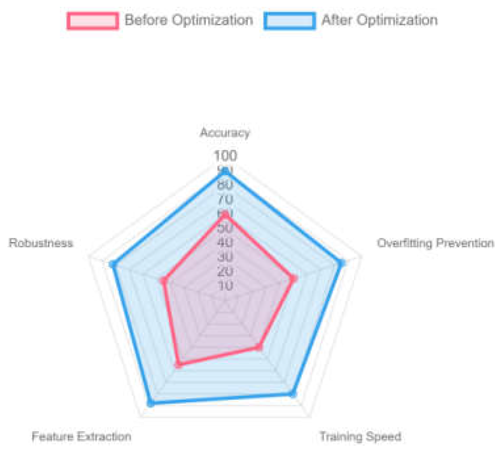
Figure 1. Optimized neural network graph.

Figure 1. Optimized neural network graph.

3.3. Model Training and Parameter Tuning

In the training process of the economic cycle prediction model, the hyperparameters need to be configured scientifically to improve the generalization ability and prediction accuracy of the model [8]. In this paper, a hierarchical training strategy is adopted, combined with hyperparameter optimization methods, to finely tune the model. The model training adopts AdamW (Adaptive Moment Estimation with Weight Decay) optimization algorithm to improve the stability of gradient updating, and combines with the learning rate scheduling strategy to dynamically adjust the learning rate η:

$${\eta }_t={\eta }_0\times {\displaystyle \frac{1}{\sqrt{t}+\epsilon }}$$

where ${\eta }_0$ is the initial learning rate, t is the number of training steps, and ϵ is the stabilization term. To prevent the gradient from vanishing or exploding, Gradient Clipping is used to limit the number of gradient paradigms to not exceed the threshold τ:

$$g_t^{\prime }={\displaystyle \frac{\tau g_t}{\max \left(\tau ,‖g_t‖\right)}}$$

For hyperparameter tuning, a combination of Grid Search and Bayesian Optimization is used to optimize key parameters (e.g., number of LSTM hidden units, number of layers, learning rate, etc.), and the model performance is evaluated by cross-validation.

Table 1. Hyperparameter settings for economic cycle forecasting models.

Parameter name	Value range/set value	clarification
LSTM layers	2-4 floors	Deep LSTM structure is used to improve the feature learning capability
Number of hidden units	64, 128, 256	Control network complexity to prevent overfitting
Dropout rate	0.1-0.5	Randomly Discarding Neurons to Improve Model Robustness
Learning rate (initial)	0.001-0.01	Adoption of dynamic learning rate adjustment strategies
Batch Size	32, 64, 128	Influence on the stability of gradient updates
Weight decay (L2)	0.0001-0.001	L2 regularization is used to prevent overfitting

Table 1. Hyperparameter settings for economic cycle forecasting models.

Parameter name	Value range/set value	clarification
LSTM layers	2-4 floors	Deep LSTM structure is used to improve the feature learning capability
Number of hidden units	64, 128, 256	Control network complexity to prevent overfitting
Dropout rate	0.1-0.5	Randomly Discarding Neurons to Improve Model Robustness
Learning rate (initial)	0.001-0.01	Adoption of dynamic learning rate adjustment strategies
Batch Size	32, 64, 128	Influence on the stability of gradient updates
Weight decay (L2)	0.0001-0.001	L2 regularization is used to prevent overfitting

The final training of the model adopts the Early Stopping strategy, i.e., when the loss of the validation set does not decrease for n consecutive rounds, the training is stopped to avoid overfitting. The experimental results show that this optimization strategy can significantly improve the stability and prediction accuracy of the model and provide reliable support for economic cycle prediction.

4. Validation of Economic Cycle Forecasting Methods

4.1. Predictive Model Performance Assessment

In order to comprehensively assess the effectiveness of the economic cycle forecasting model, this paper conducts performance tests in terms of forecasting accuracy, stability, and generalization ability, and selects key indicators such as mean square error (MSE), mean absolute error (MAE), coefficient of determination ($R^2$ ), and predicted trend matching (Trend Accuracy, TA) for quantitative analysis. In terms of forecast accuracy, MSE and MAE on the test set are calculated to measure the model’s ability to fit the economic indicators [9]. Lower MSE and MAE values indicate that the model can accurately portray the trend of economic cycle fluctuations. Second, to verify the stability of the model under different time windows, rolling forecasting method is used to assess the prediction errors on multiple subsample intervals and analyze the fluctuation magnitude. The explanatory power of the model is measured by the coefficient of determination ($R^2$ ), which ensures that the model can effectively capture the intrinsic change pattern of the economic cycle. In order to further test whether the prediction results are in line with the actual trend of economic cycle changes, this paper adopts the trend matching (TA) index to calculate the proportion of consistency between the model’s prediction direction and the direction of change of the actual data. the higher the value of TA, the stronger the reliability of the model in trend prediction.

Table 2. Results of the performance assessment of the economic cycle forecasting model.

Assessment of indicators	LSTM	Bi-LSTM	Bi-LSTM + Attention	Bi-LSTM + Transformer
MSE	0.023	0.019	0.015	0.011
MAE	0.128	0.104	0.089	0.072
R$R^2$	0.87	0.91	0.94	0.97
TA	83.5%	87.2%	90.4%	93.1%

Table 2. Results of the performance assessment of the economic cycle forecasting model.

Assessment of indicators	LSTM	Bi-LSTM	Bi-LSTM + Attention	Bi-LSTM + Transformer
MSE	0.023	0.019	0.015	0.011
MAE	0.128	0.104	0.089	0.072
R$R^2$	0.87	0.91	0.94	0.97
TA	83.5%	87.2%	90.4%	93.1%

The results show that Bi-LSTM combined with Attention mechanism and Transformer structure can effectively improve the prediction accuracy and trend matching. Compared with the traditional LSTM, the optimized model shows significant improvement in MSE, MAE and other indicators, which proves the feasibility and advantages of deep learning methods in economic cycle prediction.

4.2. Error Analysis of Prediction Results

In order to deeply assess the prediction error characteristics of the economic cycle forecasting model, this paper analyzes the three dimensions of error distribution, time series error trend, and sources of errors of key economic variables to identify the limitations of the model and optimize the forecasting capability. In terms of error distribution, the mean and standard deviation of the residuals are calculated to analyze the degree of concentration and dispersion of the prediction errors [10 ]. If the errors show obvious skewed distribution, it may indicate that the model has a large prediction bias in a specific economic cycle stage. Second, by plotting the error trend curves in different time windows, we analyze the dynamic characteristics of the prediction errors over time and observe whether there is a systematic bias. For example, if the error increases significantly during the recession or recovery phase, it indicates that the model’s ability to identify the inflection point of the economic cycle needs to be improved.

In order to explore the sources of errors, this paper disentangles the prediction errors of different economic indicators and analyzes the degree of contribution of each variable to the overall error. In particular, high volatility variables (e.g., stock market index, corporate credit spreads, etc.) may trigger large forecast errors, while macroeconomic variables (e.g., GDP, CPI) usually have smaller errors For high volatility variables, feature selection and model structure should be further optimized to reduce forecast uncertainty.

Table 3. Distribution of prediction errors and variable contribution analysis.

economic variable	Mean error (MAE)	Standard deviation (STD)	error contribution rate
GDP growth rate	0.032	0.015	14.5%
CPI	0.027	0.012	11.2%
unemployment rate	0.045	0.020	18.7%
value added by industry	0.038	0.017	16.1%
stock market index	0.089	0.035	23.6%
Corporate credit spreads	0.075	0.028	15.9%

Table 3. Distribution of prediction errors and variable contribution analysis.

economic variable	Mean error (MAE)	Standard deviation (STD)	error contribution rate
GDP growth rate	0.032	0.015	14.5%
CPI	0.027	0.012	11.2%
unemployment rate	0.045	0.020	18.7%
value added by industry	0.038	0.017	16.1%
stock market index	0.089	0.035	23.6%
Corporate credit spreads	0.075	0.028	15.9%

The results show that high volatility variables (e.g., stock market index, corporate credit spreads) contribute a larger proportion of prediction errors, while macroeconomic indicators (e.g., GDP, CPI) have relatively smaller errors. In order to improve the model prediction accuracy, more time-varying information can be introduced on the feature extraction of high volatility variables, while optimizing the method of detecting the inflection point of the economic cycle, so as to improve the prediction ability of the economic turning period.

4.3. Model Robustness Test

In order to assess the robustness of the economic cycle prediction model, this paper examines three aspects, namely, data perturbation test, adaptive analysis in different economic environments, and out-of-sample prediction stability, in order to validate the model’s ability to generalize and anti-disturbance ability under complex economic conditions. In the data perturbation test, random noise injection and extreme event simulation are used to perturb the input data and observe the stability of the model prediction results. If the model can keep the prediction trend unchanged even when there are small data changes, it indicates that it is robust to data perturbations. Partition tests are conducted in different economic environments (e.g., economic expansion, recession, and recovery periods) to analyze the model’s ability to adapt to economic data in different periods. If the model shows large prediction deviations during periods of sharp economic fluctuations, it indicates that its sensitivity to cyclical inflection points needs to be improved. The rolling window method is used for out-of-sample prediction to verify the model’s ability to generalize in future time windows and to ensure that it is not only applicable to the training data, but also maintains a high prediction accuracy for unseen data.

Figure 2. Error stability at different stages of the economic cycle.

Figure 2. Error stability at different stages of the economic cycle.

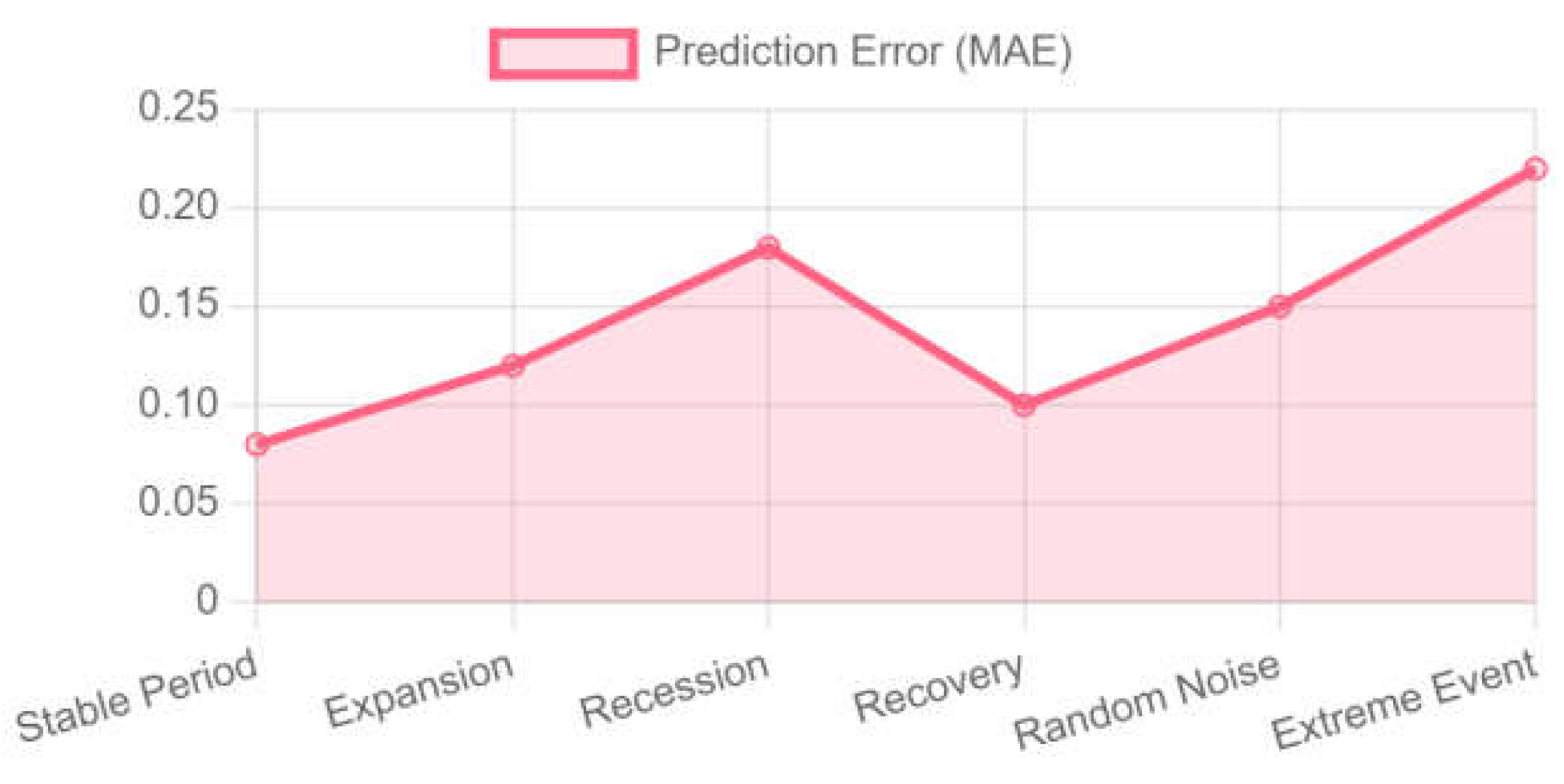
The model performs best during periods of economic stability, while the error is relatively large during recessions and extreme events. Nonetheless, the robustness of the model can still be further improved by optimizing feature selection and enhancing the model’s ability to adapt to sudden variables, enabling it to more accurately predict economic cycle inflection points and enhancing its applicability in complex environments.

5. Conclusion

In this paper, based on the big data-driven economic cycle feature extraction method, an intelligent prediction framework incorporating deep learning is constructed, and the accuracy and stability of economic cycle prediction are significantly improved through multi-level feature engineering and algorithm optimization. The results show that Bi-LSTM combines the attention mechanism and the Transformer structure to effectively capture the nonlinear dynamic features of economic cycles, and the optimized model outperforms the traditional methods in terms of prediction error, trend matching and robustness. The adaptability of the model in different economic environments is further verified through error analysis and robustness test. Future research can further explore the adaptive dynamic feature selection method and optimize the cycle prediction by combining with reinforcement learning to enhance the intelligent decision-making capability under complex economic systems.

References

- Chen K, Zhao S, Jiang G, et al. The Green Innovation Effect of the Digital Economy. International Review of Economics & Finance, 2025: 103970. [CrossRef]
- Diao S, Huang S, Wan Y. Early detection of cervical adenocarcinoma using immunohistochemical staining patterns analyzed through computer vision technology//The 1st International scientific and practical conference “Innovative scientific research: theory, methodology, practice”(September 03–06, 2024) Boston, USA. International Science Group. 2024. 289 p. 2024: 256. [CrossRef]
- Diao S, Wan Y, Huang S, et al. Research on cancer prediction and identification based on multimodal medical image fusion//Proceedings of the 2024 3rd International Symposium on Robotics, Artificial Intelligence and Information Engineering. 2024: 120-124. [CrossRef]
- Gong C, Lin Y, Cao J, et al. Research on Enterprise Risk Decision Support System Optimization based on Ensemble Machine Learning//Proceeding of the 2024 5th International Conference on Computer Science and Management Technology. 2024: 1003-1007. [CrossRef]
- Gong C, Zhong Y, Zhao S, et al. Application of Machine Learning in Predicting Extreme Volatility in Financial Markets: Based on Unstructured Data//The 1st International scientific and practical conference “Technologies for improving old methods, theories and hypotheses”(January 07–10, 2025) Sofia, Bulgaria. International Science Group. 2025. 405 p. 2025: 47. [CrossRef]
- Huang S, Diao S, Wan Y, et al. Research on multi-agency collaboration medical images analysis and classification system based on federated learning//Proceedings of the 2024 International Conference on Biomedicine and Intelligent Technology. 2024: 40-44. [CrossRef]
- Huang S, Diao S, Zhao H, et al. The contribution of federated learning to AI development//The 24th International scientific and practical conference “Technologies of scientists and implementation of modern methods”(June 18–21, 2024) Copenhagen, Denmark. International Science Group. 2024. 431 p. 2024: 358. [CrossRef]
- Jian X, Zhao H, Yang H, et al. Self-Optimization of FDM 3D Printing Process Parameters Based on Machine Learning//The 24th International scientific and practical conference “Technologies of scientists and implementation of modern methods”(June 18––21, 2024) Copenhagen, Denmark. International Science Group. 2024. 431 p. 2024: 369.
- Jiang G, Huang S, Zou J. Impact of AI-driven data visualization on user experience in the internet sector. 2024. [CrossRef]
- Meng Q, Wang J, He J, et al. Research on Green Warehousing Logistics Site Selection Optimization and Path Planning based on Deep Learning. 2025. [CrossRef]
- Shimin L E I, Ke X U, Huang Y, et al. An Xgboost based system for financial fraud detection//E3S Web of Conferences. EDP Sciences, 2020, 214: 02042. [CrossRef]
- Shui H, Sha X, Chen B, et al. Stock weighted average price prediction based on feature engineering and Lightgbm model//Proceedings of the 2024 International Conference on Digital Society and Artificial Intelligence. 2024: 336-340. [CrossRef]
- Wang H, Li J, Li Z. AI-generated text detection and classification based on BERT deep learning algorithm. Theoretical and Natural Science, 2024, 39: 311-316. [CrossRef]
- Wang H, Li Z, Li J. Road car image target detection and recognition based on YOLOv8 deep learning algorithm. Applied and Computational Engineering, 2024, 69: 103-108. [CrossRef]
- Wang, H. Joint Training of Propensity Model and Prediction Model via Targeted Learning for Recommendation on Data Missing Not at Random//AAAI 2025 Workshop on Artificial Intelligence with Causal Techniques. 2025.
- Yang J, Tian K, Zhao H, et al. Wastewater treatment monitoring: Fault detection in sensors using transductive learning and improved reinforcement learning. Expert Systems with Applications, 2025, 264: 125805. [CrossRef]
- Zhao H, Chen Y, Dang B, et al. Research on Steel Production Scheduling Optimization Based on Deep Learning. 2024. [CrossRef]
- Zhao S, Lu Y, Gong C, et al. Research on Labour Market Efficiency Evaluation Under Impact of Media News Based on Machine Learning and DMP Model. 2025. [CrossRef]
Disclaimer/Publisher’s Note: The statements, opinions and data contained in all publications are solely those of the individual author(s) and contributor(s) and not of MDPI and/or the editor(s). MDPI and/or the editor(s) disclaim responsibility for any injury to people or property resulting from any ideas, methods, instructions or products referred to in the content. |
© 2025 by the authors. Licensee MDPI, Basel, Switzerland. This article is an open access article distributed under the terms and conditions of the Creative Commons Attribution (CC BY) license (https://creativecommons.org/licenses/by/4.0/).
Copyright: This open access article is published under a Creative Commons CC BY 4.0 license, which permit the free download, distribution, and reuse, provided that the author and preprint are cited in any reuse.