Submitted:
06 April 2025
Posted:
08 April 2025
You are already at the latest version
Abstract
The researchers looks at process characteristics in order to improve color choices and create more accurate simulation models, in this research paper. The processing factors evaluated were speed (Sp), temperature (T), and feed rate (FRate). We used Box-Behnken Design (BBD) and the three-Level-Full-Factorial Design (3LFFD) response surface techniques to adjust uniform processing settings. This study employed an experimental approach to optimize process parameters while holding all other variables constant. Statistical and numerical optimization were both made possible by the Design Expert software, which also helped with experimental design. We used this technique to generate a statistical equation for simulated regression models. The optimal tristimulus color values have the smallest color variance (dE*). The created model and experimental data passed all diagnostic tests, showing that the model is statistically valid. The three examined parameters had a significant effect on the color parameters dL*, da*, and db*, as well as specific mechanical energy (SME), according to the Analysis of Variance (ANOVA). Furthermore, we calculated specific mechanical energy for the experimental trials and found that it decreased as the FRate increased. The study concludes by comparing the two design models to determine which produces the best color quality. Choosing the right process settings is crucial for reducing color fluctuations (dE*). Furthermore, during the experimental trials, we performed microscopic characterization, including agglomeration level assessments. To determine pigment dispersion, the collected data was analyzed using Scanning-Electron Microscopy (SEM) as well as Micro-CT-scanner pictures (MCT). This work contributes to addressing potential design and manufacturing difficulties that affect color variability and waste minimization for diverse chemical grades, thereby encouraging environmentally friendly operations. Regarding the BBD. The processing circumstances indicate that 728.38 rpm, 274.23 °C, and 24.44 kg/hr are closest to the target specifications. In addition, overall the lowest deviation=0.26 while 87% is the maximum design attractiveness. We are discussing the three-Level Full Factorial Design (3LFFD). Generally the a maximum desirability of 77% and a minimum tolerable color variation (dE*) of 0.25, we determined that 741.27 rpm, 245.26 °C, and 24.72 kg/hr were the ideal process parameters. These results show that the processing parameters used to generate the output have a significant impact on its quality. To reduce the variation and improve appeal more modifications This study compares the two generated designs and discovers that both sets of process parameters were statistically significant, with BBD being the preferred option for selection needed, resulting in even better outcomes in future experiments.
Keywords:
Polycarbonate
; Interaction for processing Parameter’s
; Optimization
; Simulation
; (3LFFD) and (BBD)
; Regression models
; Microscopic Characterization
1. Introduction
Polymer resins, in their unaltered form, fulfill numerous performance criteria but lack the coloration that appeals to consumers. Creating plastic that a commercially viable color necessitates the use of, in general, more than one pigments; yet, attaining the desired hue on the initial attempt is a significant hurdle. Nevertheless, getting the right shade on the first try could be quite difficult. There are a lot of factors that affect how polymers look. Screw speed and screw design, temperature FRate, and residence time all play a role in their extrusion process. Several studies have looked at how different process variables affect the final color of polymer compounding [1,2]. Due to the pigment’s chemical composition, it is highly probable that they will experience specific chemical reactions that will depend on the specific process circumstances. Moreover, the polymer's characteristics may be impacted by the substantial link between time and temperature. Therefore, the desired hue need a carefully chosen variables from our researchers. To achieve the required pigment dispersion and ideal homogeneity, reduce the resin's viscosity and increase the mixing time [3]. When it comes to quality assurance, color measurement, and numerical comparison of color changes, spectrophotometers are indispensable [3]. For polycarbonate grade-3, we established limitations for dE at or below 1.0 and for dL*, da*, and db* at or below 0.6, although in most cases, customers decide what is considered a suitable tolerance limit [4]. The "dE*" represents the dispersion in (b*) (L*), & (a*):
(dE*) = [(dL* 2) + (da* 2) + (db* 2)]
In place of utilizing color values that are absolute, color differences concerning target values regarding dL*, da*, and db* are used. We represent the color difference in the CIELAB color space using the total change in color, dE* [5].
This study states these challenges by examining the effects of various processing conditions on PC blends with additives and composites, focusing on color consistency. This study finds the best ways to use statistical tools like DOE and processing parameters to improve the quality and accuracy of color in colored polymer products. It accomplishes this by extrusion, blending, and color testing, studying their rheology and RSMs, and looking at their surface morphology and microstructural characteristics. With the rising importance of sustainability and preparing the way for advanced solutions that develop color consistency and execution [6,7,8].
Reducing waste and expediting material delivery are the largest challenges facing polymer compounders; compounding is the process of homogeneously mixing pigments in predetermined amounts and ratios to create the desired color. These pigments, typically different colors, reflect the incident light at various depths, resulting in the desired color being seen as the result of the combined effect of reflection [9,10].
Color deviations can result from a variety of factors, such as differences in formulations or pigment dispersions and the effects of processing parameters on material performance; examine the results of these variations in color combinations when compounding is a unique opportunity. According to the CIE, L*, a*, and b* color values were obtained using a spectrophotometer [11,12].
This study looks at process characteristics in order to improve color choices and create more accurate simulation models. Feed rate (FRate), Speed (Sp), & Temperature (T) were the processing variables examined. We used the 3-Level- Full-Factorial Design (3LFFD) as well as (BBD) response surface techniques to adjust uniform processing in three levels. This study employed an experimental approach to optimize process parameters while holding all other variables constant. The Design Expert software facilitated experimental design while also allowing for statistical and numerical optimization. We used this technique to generate a statistical equation for simulated regression models. The optimal tristimulus color values have the smallest color variance (dE*). The created model and experimental data were passed all diagnostic tests. Statistically, these tests show that the model is valid . We have confirmed the model's statistical validation when all diagnostic tests were passed by both the created model and the experimental data.
The dL*, da*, and db* color parameters and the specific mechanical energy (SME) were all significantly impacted by the three parameters that were considered in the Analysis of Variance (ANOVA). Furthermore, we calculated specific mechanical energy for the experimental trials and found that it decreased as the Frate increased. The study concludes by comparing the two design models to determine which produces the best color quality.
Choosing the right process settings is crucial for reducing color fluctuations (dE*). Furthermore, during the experimental trials, we performed microscopic characterization, including agglomeration level assessments. To determine pigment dispersion, the collected data was analyzed using SEM as well as Micro-CT scanner pictures (MCT). This work contributes to optimize potential modelling design and manufacturing difficulties that affect color variability and waste minimization, for diverse chemical grades; hence, encouraging environmentally friendly operations.
The addition of additives to polymeric components may have led to unforeseen effects on their viscosity, mechanical processing, properties, and visual appearance [13,14]. A multitude of studies has explored the incorporation of color into virgin resin. In the experiment, we used the Response-Surface Method (RSM). This method included different processing conditions and three levels of process variables. When we optimally combined (FRate, T & Sp) values under specified processing conditions, we observed a deviation which is slight comparing to the expectation of the color output [15,16,17,18].
On top of that, the Response-Surface Method (RSM) generates new insights, improves material performance, and makes it possible to investigate intricate interrelationships. RSM has recently achieved remarkable achievements in enhancing the performance characteristics of polymer materials through statistical modeling and property refinement in PC composites. Using RSM has been shown to improve the performance of polycarbonate nanocomposites by looking at how key factors that affect material properties interact with each other [19,20].
To investigate the color variations caused by changes in processing parameters, we employed the Statistical Design of Experiments. Techniques such as Response Surface Methodology (RSM) facilitate this process. Careful experimental design to evaluate model parameters after execution is the first step in this process; then formulate a second-order polynomial for the responses [21].
Design of trials (DOE) is a systematic methodology enabling an investigator to organize trials and ascertain cause-and-effect correlations. Because it decreases the necessary number of tests, DOE is actively used by several scientific areas. Improving the extrusion process parameters is key to getting these pigments dispersed evenly. A compounded polycarbonate grade's color characteristics were the subject of investigations to determine process parameters’ impact over these features. Therefore, we decided to build a regression model. The color disparity was caused by a myriad of factors. Understanding how these factors affect the final hue requires investigation of these factors [21,22].
In order to optimize process variables, many different experimental designs have been found to be effective. The impact on PVC-sheets' surface look and gloss with varying compounding process factors was studied using a modified general factorial Design of Experiments (DOE) [23]. Some examples of RSM designs are: the factorial, the Central-Composite Design: CCD, the BBD, and the D-optimal [24]. Research has shown that a DOE using the BBD may determine the relationship between processing factors and the variance in wood-plastic matrix viscosity [25].
As a combined array design, the Box-Behnken Design (BBD) streamlines the computation of substantial interactions and reduces the number of runs needed compared to Taguchi's crossing array designs [26]. With this method, you can construct a quadratic model with just three levels per factor, and it is quite economical in terms of runs [26,27]. Some designs, like a Central Composite Design (CCD) with five levels of each element or a Three-Level Factorial Design with potentially more trial runs, are required to estimate curvature.
To determine the produced quadratic model's usefulness and importance, as well as the model's suitability, an analysis of variance (ANOVA) is necessary. The process parameters' impact and how they interact were examined in the study. By giving careful thought to error propagation (POE), RSM designs become more dependable. When calculating POEs—the standard deviation of changes in output’s responsiveness resulting from, during experimentation, significant controllable process factors changes [28]; we do not think noise is a big deal.
The processing parameters are thoroughly analyzed using design of experiments (DOE) in this study. Finding out how many tests would be necessary to collect enough data for a thorough study became much easier with the help of DOE. We designed the systems with processing speed, FRate, temperature, and accuracy in mind. We looked at how the parameters of the output response changed depending on the processing settings. To learn how the color of compounded plastics changed as processing parameters were adjusted, the researchers ran systematic testing on different grades; we looked over the data to find the optimal processing parameters for reducing waste while guaranteeing on-time order delivery.
If you want to find out how different processing settings affect color, you can use Statistical Design of Experiments (DOE) with approaches like RSM. In order to efficiently evaluate our model factors, some researchers have been implementing, the first step is to carefully prepare the experiments, followed by the recreation of a second-order polynomial to stand in for the replies [27,28].
The expected outcome is represented by y in this context, while the remaining values are as follows: b0: a constant, bii: the ith-quadratic coefficient, bi: the ith-linear coefficient, bij: the ith-interaction coefficient, k: # of factors, ε: the error, and xi: the independent variable. The model's coefficients are predicted by regression analysis of the collected experimental data. Some researchers have outlined the methodology used to estimate the model's parameters in their subsequent publications [27,28]. Optimization, process improvement, and development can all benefit from RSM's statistical and mathematical approaches. One of the most powerful and successful response surface methods is the 3LFFD when compared with others like Central Composite, Doehlert matrix, and BBD. We aim to utilize a three-LFFD. This design determines the optimal processing settings that minimize color disparities (dE* < 0.8).
A lot of research has looked at how processing parameters affect properties like water permeability and salt rejection, and ANOVA has confirmed those findings. Design of Experiment (DOE) models show how these parameters affect material properties, which helps to optimize pigment and polycarbonate mixes for better performance. We created supplementary models utilizing the Design of Experiments methodology. On the other hand, polyacrylic acid-graphene-oxide, a compound with multiple applications, had their synthesis parameters optimized using Response-Surface Methodology (RSM). Results from further analyses of variance (ANOVA) validated the models [29,30,31,32].
To get consistent color properties in plastics, this research looks at mixing two polycarbonate resins. Optimizing for speed, temperature, and FRate, this study employs DoE and RSM to see how pigment dispersion is affected. Improved production of colored polymer goods is the result of its use of prior industry data that addresses color consistency difficulties [33,34]. Some researchers argue that when Polycarbonate (PC) mixed with Low-Density Polyethylene (LDPE) may reduce the overall viscosity, allowing the components to glide about during injection molding, therefore improving the process [35]. The study concludes by looking into letdown and pigment dispersion and how they are affected by the processing temperature to growth ratio in polymer matrices. It examines thermal stability plus viscosity parameters [36].
SEM offers critical invaluable information about polycarbonate blends' characteristics (in particular, the microstructural ones), especially for examining agglomeration as well as pigment dispersion. The findings demonstrate significant shear thinning exhibited by Acrylonitrile-Butadiene Styrene (ABS), while, Polycarbonate (PC) largely exhibits Newtonian behavior [37,38]. In emulsions of polymers with a high viscosity: surface morphology, particle size, as well as distribution are studied in this report using a structured approach to Scanning Electron Microscopy (SEM). This method effectively solves the issues related to high-viscosity SEM analysis, giving a clear picture of the emulsion's microstructure at different viscosities [37,38].
Researchers also use scanning electron microscopy (SEM) to find out how pigment dispersion quality affects color uniformity. They find that consistent dispersion reduces color variations and clumping [39]. Researchers broadened their scope to investigate the variations in autonomous processing characteristics. For consistent output color, researchers used variables like speed, FRate, temperature to influence the dependent responses (L*, a*, b*, dE). When you compare the three-level full factorial and BBD designs to other methods, for example, BBD, the central composite, as well as Doehlert matrix, they considered the most powerful and effective response-surface.
Focusing on polycarbonate matrices specifically, this study aims to examine pigment dispersion-processing factors-color consistency interplay in compounded plastics. This work methodically optimizes pigment-mixing processes using two separate methodologies: RSM as well as DOE. This investigation enhances our understanding of consistency as well as color stability and how they impacted by processing conditions. Researchers’ concentration is enhancing the process of blending various pigments and additives with two polycarbonate resins. The extrusion speed (650, 750, and 850 rpm), temperature (230, 255, and 280 °C), and FRate (11, 19, and 27 kg/h) will be systematically varied during 17 Box-Behnken Designs (BBD) runs. Furthermore, we perform 32 experimental runs in 3LFFD, systematically adjusting the extrusion where Sp: 700 rpm, 750 rpm, and 800 rpm, T: 230 °C, 255 °C, and 280 °C while FRate: 20 kg/h, 25 kg/h, and 30 kg/h. we are Utilizing the software(version eight) of Design-Expert. Therefore, optimize the most effective design by analyzing the significant interactions of processing parameters in order to improve the accuracy of first-pass color while reducing color variability. Using both microscopies, the multi-mode (MCT) as well as scanning electron (SEM) scanning analysis, we will determine the effects of dispersion on the chemical and physical structures of the materials. In addition, we will verify the density of the agglomerations and the color consistency of the processed materials. The main goal is to find a correlation between processing parameters and color outputs so that color formulations can be more reliably improved. Our goal focuses on utilization as well as the comparison of two designs to optimize processing parameters, aiming for minimal deviation in color properties (dE* < 1.0). We will conduct further characterizations to assess the structure and efficiency of color dispersions. Optimal colors were determined and statistically significant models were generated by both designs.
2. Materials and Methods
At the industrial plant, we carried out trials on the material under investigation. As detailed in Table 1, a combination of various pigments and two PC resins was utilized, with these grades’ color formulation expressed in Parts per Hundred (PPH). A value of 6.5 g/10 min exhibited for Resin 2, whereas Melt-flow-index: MFI recorded at 25 g/10 min for Resin 1.
Given its 37:1 length-to-diameter ratio, 25.5 mm diameter, and a diameter (Do/Di ) ratio of 1.55, we ran the material extrusion process using a co-rotating (27-kW) Twin-Screw-Extruder (TSE): innovative intermeshing designs from Germany, ZSK26. Nine heating zones were located on the extruder's barrel while one was located at the die. After extruding the melt, we cooled it with cold water. Secondly, we allowed it to air dry, and thirdly, we pelletized it. Three rectangular chips measuring 3x2x0.1" were formed from the pellets from each run by injection molding. Then we used an American X-Rite spectrophotometer (CE: 7000A) to measure as well as (CIE L*, a*, b*)
In this case, L* = 70.04, a* = 3.41, and b* = 18.09 would produce the intended color result. We included three process parameters in the experimental design, as shown in Table 2: extruder FRate, heating zone temperature, and screw speed. Utilizing the eighth version of American Design Expert Software (Stat-Ease, Inc.), we quantitatively assessed the data and established correlations among the variables at a 95% confidence interval through statistical analysis. To make sure the data stayed true to the target color, we optimized it numerically. We used a ratio of 100:0.86 to combine the resins and additives in Figure 1. A super floater batch blender blends them according to weight ratios to make the mixture more consistent [40,41].
In the experimental design, the three different levels denoted by the code (-1, 0, and +1) for each element, as presented in Table 2, assessed the same three process parameters. Both experimental designs took into account the utilization level in addition to the extruder FR, speed, and temperature, as indicated in Table 2.
We prepared the batches using additives and pigments. Using the transparent PC grade material we created; we studied processing parameters and formulation's influence on changes in the final appearance of color and characteristics. By examining these results as well as the roles played by the dispersion morphologies of the three processing parameters, we gained a better understanding of the factors that create color disparities. Figure 2 displays a simplified flow diagram that illustrates the steps involved in the compounding process. This illustration highlighting the relationships between various parameters and their impact on the final product's color and characteristics. By visualizing these connections, we can better understand how adjustments in processing can lead to different outcomes.
2.1. The Effects of Processing Parameter Interactions
The production of an accurate color through injection necessitates an appropriate operational procedure because the color variations will be affected by any changes in the processing parameters. The present study employed a systematic approach to manipulate the operational factors in order to examine their impact on pigmentation. We independently modified, (the speed, the rate of flow (FRate) & temperature) processing parameters across three separate stages. We noted when we held all other variables constant, we found that coloration was significantly correlated with the processing parameters. The experiments were conducted in the following manner: The recommended processing conditions included a steady speed (750 rpm) and an FR (25 kg/hr) and three distinct temperatures (280°C, 255°C & 230°C); then we repeat same processing for the speed and the rate of flow (FRate). This study utilizes two designs of the Response Surface Method (RSM).
2.1.1. Three Level Full Factorial Design
A total of twenty-seven independent experimental runs make up the initial Design of Experiments (DOE), each with an additional five center points to accommodate differences in processing parameters. This results in a total of 32 treatments, as illustrated in Table 5 and Figure 3a.
2.1.2. Box Behnken Design (BBD)
Table 6 and Figure 3b display the second Design of Experiments (DOE). The second Design of Experiments (DOE) includes 12 experimental runs and five additional center points to accommodate various processing parameters, resulting in a total of 17 treatments. The experimental design took into account three process parameters: the extruder’s screw speed, FRate as well as the heating zones’ temperature, the extruder’s screw speed as well as FRate, with Table 2 displaying the levels used. We varied the parameters on 12 different treatments. To see how they affected color, we added, for the BBD response method, five additional center points. Then, for the sake of detecting nonlinearity in the responses and estimating the experimental error, we added the additional five center points.We also recorded the percentage load during the experimental runs to calculate the specific mechanical energy (SME) using equation 3 [42].
where: P: Power (kW); nm: Max. Screw rotations (rpm); O: Load (%); n: Screw rotations (rpm); Q: FRate (kg/h).
The extruder’s screw speed, FRate as well as the heating zones’ temperature. Here, a control study has been conducted for examining the screw speed, FRate as well as temperature’s effects on color, as these factors directly influence it. We individually controlled three processing parameters at different stages. Here, we fixed the FR and temperature at middle values, and then we chose speeds of 700, 750, and 800 rpm. Then, we repeat the same procedure for the rate of flow (FRate) and temperature; our observation confirmed a significant color-processing variables correlation. We consider the above factors, which help us zero down on the best process parameters to make the plastic grade consistently colored [43].
The study employs various scientific design techniques to minimize material rejects during the initial batch of color evaluations. Its primary objective is to investigate the interactions between FRate, temperature, screw speed, and trismillus color variants, as well as the processing conditions' effects. To maximize our processing parameters’ effect, we employes two experimental designs, and subsequently presented a statistical comparison of both designs. There are three steps to these statistical procedures study: Here we take a look at how color output and FR, temperature, and screw speed interact with one another. We compare the two designs using tools like ANOVA, overlay plots, and desirability graphs. This research examines the specific mechanical energy process in detail. We measured the colors in the experiments. We used MCT as well as SEM microscopes to examine pigments’ morphology in PC compounds. We also used them to look into the shape, dispersion quality, and color consistency-PC compound quality of pigments correlation.
3. Discussion and Results
This study looks at two model designs: (3LFFD) as well as (BBD). First, we must present the ANOVA results so that we may develop a valid and significant model.
3.1. Analysis of Variance: ANOVA
To find out how things interacted and to tweak the color processing parameters, we ran an ANOVA. We thoroughly investigated how different characteristics affected dL*, da*, db*, and SME using DOE. We Started by a linear model and progressively more terms were added, whether linear or quadratic, according to the requirement, we conducted sequential F-tests [44]. We calculated each model type’s F-statistic to select the highest-order-significant terms one [30]. We followed a similar methodology across all tristimulus values, including only the significant terms identified by: F≤ 0.05 and probability values ≤ 0.1. The result of ANOVA (for the sequential model sum of squares) in Table 3, include: dL*, da*, db*, and SME. The highest-order models with significant terms are the quadratic model, as indicated by a Prob > F value of less than 0.05. As a result, these models accurately characterize dL*, da*, and db*, as well as SME responses. The adjusted R2 values provided in Table 3 supported this observation.
Conversely, keep in mind that just because quadratic models are common doesn't mean they're useful in real-world contexts. Furthermore, although the Prob > F values suggest statistical significance, they do not account for the potential risks of overfitting or the complex interrelationships among the variables
The components normally explain only 72% of the variation in db*, while the variation in da*, dL*, & SME equal 90%, according to R2 in BBD. The components in 3LFFD typically account for about 78% of the difference in db*, da*, & dL*, as evidenced by R2. However, the figure drops to 75%.
There is no explanation for the residual variability in the responses. The term "noise" could be used to describe these unforeseen variations. reasonable agreement is very clear between the "Predicted R2 " and the "Adjacent R2 ". "Adequate precision" is a metric that measures the ratio of noise to signal; ideal values surpass four. The ratio > 4 suggests that the design space may be successfully traversed by the model. In order to compare the pure as well as residual error, we employed the test: "lack of fit". We found that the result is not statistically significant because the p-value, of "lack of fit", > 0.05. The F-value indicates statistical significance compared to noise, whereas the modest p-value (< 0.05) indicates meaningful model terms. The R² -value and adjusted R² -value illustrate that values nearer to one suggest a better match [30].
3.2. Regression Models for Trismilus Color and SME
Table 4 displays the (ANOVA) results, which enabled the generation of multiple-linear-regression models for dL*, da*, db*, and SME prediction. Coefficient values demonstrate the extent to which process variables (FRate, speed, and temperature) impacted responses; polynomial equations mathematically depict these variables and their interactions. Table 5 and Table 6 display the tiny variations between the predicted and actual color responses, indicating a significant agreement.
Response surface curves (RSM) utilize variations in color value yield as a function of two process factors, while keeping the third factor constant. The determination of optimal settings for process parameters, along with the analysis of their relationships, is facilitated by the use of RSM curves

Table 5.
Comparison: Actual-pred.-values of dL*, db* and da*for (3LFFD).
| (Run) | (dL*) | (da*) | (db*) | (Pred & Actual & color value Difference) | |||||
| (Actual) | (Pred) | (Actual) | (Pred) | (Actual) | (Pred) | dL* | da* | db* | |
| 1 | -0.520 | -0.50 | 00.61 | 00.57 | 00.31 | 00.14 | -00.02 | 00.04 | 00.17 |
| 2 | 00.16 | 0.093 | 00.23 | 00.12 | -00.17 | -00.25 | 0.067 | 00.11 | 00.08 |
| 3 | -0.59 | -0.57 | -0.3 | -0.087 | -0.76 | -0.34 | -0.02 | -0.213 | -0.42 |
| 4 | 0.11 | -0.2 | 0.29 | 0.003 | -0.22 | -0.4 | 0.31 | 0.287 | 0.18 |
| 5 | 0.01 | -0.24 | -0.16 | -0.059 | -0.16 | -0.49 | 0.25 | -0.101 | 0.33 |
| 7 | -0.65 | -0.36 | -0.29 | 0.12 | -0.77 | -0.25 | -0.29 | -0.41 | -0.52 |
| 8 | 0.14 | -0.029 | 0.34 | 0.3 | -0.11 | 0.0081 | 0.169 | 0.04 | -0.1181 |
| 9 | -00.53 | -00.47 | 0.027 | 0.024 | -00.38 | -00.16 | -00.06 | 0.003 | -00.22 |
| 10 | 0.087 | -0.18 | 0.14 | 0.03 | -0.18 | -0.4 | 0.267 | 0.11 | 0.22 |
| 11 | -0.21 | -0.087 | 0.077 | -0.087 | -0.56 | -0.34 | -0.123 | 0.164 | -0.22 |
| 12 | -0.44 | -0.54 | 0.65 | 0.24 | 0.37 | -0.099 | 0.1 | 0.41 | 0.469 |
| 13 | 0.25 | 0.41 | 0.27 | 0.24 | -0.14 | -0.099 | -0.16 | 0.03 | -0.041 |
| 14 | -00.55 | -00.23 | -00.15 | -0.059 | -00.55 | -00.49 | -00.32 | -0.091 | -00.06 |
| 15 | -00.71 | -0.20 | -00.05 | 0.031 | -00.93 | -00.40 | -00.51 | -0.081 | -00.53 |
| 16 | -0.53 | -0.4 | -0.12 | -0.031 | -0.84 | -0.64 | -0.13 | -0.089 | -0.2 |
| 18 | -0.34 | -0.26 | -0.22 | 0.024 | -0.35 | -0.16 | -0.08 | -0.244 | -0.19 |
| 19 | 0.037 | -0.065 | 0.29 | 0.24 | -0.22 | -0.099 | 0.102 | 0.05 | -0.121 |
| 20 | -0.48 | -0.49 | 0.65 | 0.3 | 0.37 | 0.0087 | 0.01 | 0.35 | 0.3613 |
| 21 | -00.20 | -00.33 | -0.017 | -0.087 | -00.33 | -00.34 | 00.13 | 00.07 | 00.01 |
| 22 | 00.43 | 00.43 | 00.32 | 00.30 | 0.013 | 0.008 | 0.00 | 00.02 | 0.005 |
| 23 | 0.027 | -0.13 | 0.24 | 0.12 | -0.24 | -0.25 | 0.157 | 0.12 | 0.01 |
| 24 | 0.087 | 0.2 | 0.24 | 0.57 | -0.16 | 0.14 | -0.113 | -0.33 | -0.3 |
| 27 | -0.04 | -0.13 | 0.05 | 0.12 | -0.31 | -0.25 | 0.09 | -0.07 | -0.06 |
| 28 | -0.15 | -0.13 | 0.12 | 0.12 | -0.013 | -0.25 | -0.02 | 0 | 0.237 |
| 29 | -0.19 | -0.13 | 0.093 | 0.12 | -0.083 | -0.25 | -0.06 | -0.027 | 0.167 |
| 30 | -0.02 | -0.13 | -0.087 | 0.12 | -0.02 | -0.25 | 0.11 | -0.207 | 0.23 |
| 31 | -0.1 | -0.13 | -0.09 | 0.12 | -0.06 | -0.25 | 0.03 | -0.21 | 0.19 |
| 32 | -0.033 | -0.15 | 0.13 | -0.031 | -0.32 | -0.64 | 0.117 | 0.161 | 0.32 |
Table 6.
Comparison: Actual & pred. of dL*, db* and da* values for (BBD).
| (Run) | (dL*) | (da*) | (db*) | (SME) | ( Pred. & Actual color value Difference) | |||||||
| Actual | Pred. | Actual Value | Pred. | Actual | Pred. | Actual | Pred. | dL* | da* | db* | SME | |
| 1 | -0.12 | -0.062 | -0.017 | -0.02 | -0.36 | -0.24 | 0.46 | 0.45 | -0.06 | 0.006 | -0.12 | 0.01 |
| 2 | -0.26 | -0.2 | 0.07 | 0.038 | -0.27 | -0.43 | 0.75 | 0.76 | -0.06 | 0.032 | 0.16 | -0.01 |
| 3 | 0.27 | 0.18 | 0.63 | 0.6 | 0.39 | 0.18 | 0.47 | 0.45 | 0.09 | 0.03 | 0.21 | 0.02 |
| 4 | -0.037 | 0.006 | -0.043 | 0.012 | -0.34 | -0.2 | 0.49 | 0.48 | -0.04 | -0.055 | -0.14 | 0.01 |
| 5 | 0.006 | -0.025 | -0.027 | -0.04 | -0.29 | -0.39 | 0.34 | 0.35 | 0.031 | 0.017 | 0.1 | -0.01 |
| 6 | 0.3 | 0.18 | 0.65 | 0.6 | 0.39 | 0.18 | 0.47 | 0.5 | 0.12 | 0.05 | 0.21 | -0.03 |
| 7 | 0.12 | 0.18 | 0.58 | 0.6 | -0.003 | 0.18 | 0.47 | 0.47 | -0.06 | -0.02 | -0.183 | 0 |
| 8 | 0.51 | 0.59 | 0.38 | 0.36 | 0.14 | 0.14 | 0.5 | 0.5 | -0.08 | 0.02 | 0 | 0 |
| 9 | -0.1 | -0.1 | 0.11 | 0.13 | -0.31 | -0.25 | 0.77 | 0.76 | 0 | -0.02 | -0.06 | 0.01 |
| 10 | 0.15 | 0.18 | 0.58 | 0.6 | -0.047 | 0.18 | 0.47 | 0.48 | -0.03 | -0.02 | -0.227 | -0.01 |
| 11 | 0.59 | 0.52 | 0.36 | 0.33 | 0.11 | 0.094 | 0.49 | 0.47 | 0.07 | 0.03 | 0.016 | 0.02 |
| 12 | 0.47 | 0.56 | 0.36 | 0.4 | -0.023 | -0.05 | 0.38 | 0.37 | -0.09 | -0.04 | 0.025 | 0.01 |
| 13 | 0.2 | 0.18 | 0.57 | 0.6 | 0.37 | 0.18 | 0.47 | 0.46 | 0.02 | -0.03 | 0.19 | 0.01 |
| 14 | 0.55 | 0.57 | 0.32 | 0.33 | 0.12 | 0.19 | 0.35 | 0.34 | -0.02 | -0.01 | -0.07 | 0.01 |
| 15 | 0.36 | 0.39 | 0.29 | 0.3 | -0.13 | -0.09 | 0.8 | 0.79 | -0.03 | -0.01 | -0.043 | 0.01 |
| 16 | 0.19 | 0.14 | 0.2 | 0.17 | -0.22 | -0.17 | 0.36 | 0.35 | 0.05 | 0.03 | -0.05 | 0.01 |
| 17 | 0.53 | 0.469 | 0.37 | 0.36 | 0.15 | 0.202 | 0.77 | 0.78 | 0.061 | 0.01 | -0.052 | -0.01 |
3.3. Interaction of Feed Rates (FRate) and Speed for Tristimulus Color Values
To compare the two designs, we used the three-level factorial design (3LFFD) and BBD for the processing parameters. Processing parameters’ influence, particularly: (Sp & FRate), on the Tristimulus color values of polymer color chip samples is the primary focus of this comparison and in-depth analysis. This interaction is critical for assuring the final color consistency of polymer-plastic products during the production process. We intend to explore these two variables in order to identify the optimal processing settings for generating exact and consistent color results, using Tristimulus color values for measurement and computation.
3.3.1. Interaction of Speed and FRates for dL*
Figure 4a, at 274.4°C, the design interactions in BBD provide a contour graph showing the FRate and speed relationship for dL*. In contrast, at 245.2 °C, 3LFFD-Figure 4b depicts the link between speed and FRate. The FRate and speed non-linear complex relationship is illustrated in BBD's Figure 4a. When (24.4) kg/hr and (728) rpm, dL* is -0.01: the global best value. In contrast, 3LFFD-Figure 4b shows that the worldwide (dL*): ideal value equal 0.0 in particular at 245.2 °C, 24.71 kg/hr, and 741.2 rpm. Additionally, using a 95% confidence interval, the lowest possible value of dL* is -0.11, while the maximum possible value is 0.11.
3.3.2. Interaction of Speed and FRates For da*
Figure 5a shows the BBD contour map of the speed-FRate interaction at 274°C, in contrast, the 3LFFD-Figure 5b, shows the speed-Frate interaction for da*, demonstrating the first-order link between speed and FRate particularly when 245.2 °C. In Figure 5a, the BBD elliptical shapes with a large radius of curvature are produced by the quadratic components of the three processing parameters.
This indicates that as FRates and speeds rise, the da* value decreases in two quadrants and increases in the other two. Furthermore, of the four quadrants, two exhibit positive interactions between FRates and speeds, while the remaining two display negative interactions; these positive interactions underscore the potential for optimized performance. Conversely, as shown in 3LFFD-Figure 5b, experimenting with different FRates and speeds can assist in reaching the objective. In this case, a 95% confidence interval indicates that da* = 0.15 at 24.7 kg/hr at 741.2 rpm, with 0.07 being the lowest acceptable value and 0.23 being the maximum; these findings help researchers to go further in their experimentation, providing significant productivity and efficiency.
3.3.3. Interaction of Speed (Sp) and Feed Rates (FRate) for db*
Figure 6a in BBD, illustrates db* speed-FRate relationship when 274.4°C demonstrating a considerable non-linearity level, similar to dl*. On the other hand, Figure 6b, 3LFFD, at 245.2 °C, illustrates speed-FRate relationship for db*. The behavior is highly linear, with only speed and FRate serving as major model variables in comparison to (dL* & da*)[30].
Figure 6a in BBD Notable finding for db* (approaches zero), while maintaining a temperature of 274.4°C in both cases, at around 23 kg/hr FRates and the speeds at the highest, and around a FRate of 15 kg/hr while speeds is the lowest. db*equal 0.19 (as the anticipated value), at the global optimum. On the other hand, Figure 6b, 3LFFD, Notably, db* approaches zero at lower speed and FRate values around 20 kg/hr, as well as at higher values around 24 kg/hr, all while maintaining a temperature of 245.2 °C. At the global optimum, the anticipated value of db* is -0.19, with the permissible lowest and maximum values at a 95% confidence interval being -0.33 and -0.06, respectively [30].
3.3.4. Speed - FRate Interaction for SME
From an energy consumption perspective, the specific mechanical energy is crucial and should be kept to a minimum for economic reasons. The specific mechanical energy is dependent mostly on FRate and speed [44]. According to Figure 7, a contour plot showing FRate-speed relationship for a given amount of mechanical energy. Figure 7 demonstrates that an increase in FRate casing a decrease in specific mechanical energy, whereas an increase in speed barely affects it.
3.3.5. Desirability Processing Interactions for RSM
Some experts argue that it is necessary to have a multi-criteria decision-making strategy due to the significant influence of these parameters (FRate (C), speed (B), & temperature (A)) on the outcomes [45]; however, this strategy could complicate our analysis. We used a total-desirability function "d" to find the best values for these three factors in each solution [45]. The desirability function shows the desired ranges for each response (di) and provides an overall quality score. It makes it simple to compare many responses in order to choose the most desirable characteristics [30]. We translate the measured responses into a dimensionless desirability scale by calculating scales from d = 0 (an entirely undesired reaction) to d = 1 (a fully wanted answer). We achieve the best outcomes when all criteria combine optimally on a global scale. Assuming a FRate equal 24.44 kg/hr, Figure 8a depicts a three-dimensional plot of global desirabil Our findings suggest that at 24.44 kg/hr, 274.23°C, and 728.38 rpm, the combined desirability peaks at 87%. At roughly 255°C for temperature and 775 rpm for speed, the desire hits its peak, with a maximum value of around 0.87. The statistics also demonstrate that the desirability peaks are highest in the ranges' centers and lowest at their edges. The trend illustrates a correlation between departures from these temperature and speed thresholds and proportional decreases in desirability.
Figure 8b depicts a three-dimensional plot of global desirability (D) using a FRate equal 24.7 kg/hr. We identified the best operating parameters for achieving a maximum combined desirability of 77%: 245.2°C, 741.2 rpm, and a FRate equal 24.7 kg/hr. The remaining experimental domain displays diminishing d values. For example, in Figure 8b, it is obvious that higher and lower FRates and speeds have a greater impact on attractiveness than temperature vs. speed.
3.3.6. Graphical Optimization (Overlay Plots) for RSM
When a FRate equal 24.44 kg/hr, Figure 9a. BBD displays an overlay plot of response contours that illustrate speed against temperature, allowing you to see the range of possible values in the illustration. To get the mean responses (dL*, da*, db*) at a FRate equal 24.44 kg/hr, the contours with db*=0.20 and da*=0.30 bordered the region, showing the ideal speed and temperature parameters. At 274.23°C, 728.38 rpm, and 22.44 kg/hr, we achieved the best tristimulus values—dL* = -0.01, db* = -0.19, da* = 0.18, and SME = 0.389. When compared to the highest allowable deviation, dE* = 1.0, the overall minimum tristimulus values' deviation of 0.26 obtained from Equation 1, which falls within the permitted range [30]
An overlay plot of response contours with speed vs. FRate at 245.2 °C is shown in Figure 9b 3LFFD. It shows the possible values. For FRate that equal 24.44 kg/hr, the speed as well as the temperature operating parameters that meet the mean responses (dL*, da*, db*) are shown by the area between the contours of db*=0.20 and da*=0.30; when (741.2 rpm, 22.7 kg/hr, & 245.2 °C). We achieved the optimal tristimulus values are da* = 00.15., dL* = 00.0, db* = -00.19, and dE* = 1.0, in comparison to the highest allowable deviation, the overall minimum deviation in tristimulus values of 0.25 that was produced by Equation 1 is considered to be rather acceptable [30].
3.3.7. Optimization of Processing Parameters and Desirable Color Outputs: A Design Methodology
Table 7 displays the ideal conditions, color output (∆E*), necessary processing parameters, and attractiveness. This analysis compares two design methodologies: a 3-level-factorial-design with (BBD).
1. At 274°C, 728 rpm, and 24.4 kg/h, we achieved the best results using the Box-Behnken Design (BBD) specifications. The total number of runs completed is 17, and the desirability is 87%, which indicates a superior level of optimization. A lot depends on the processing parameters, especially the relationship between FRate and speed for all color values (dl*, da*, and db*). The resultant color output (dE*) is 0.26, according to our calculations.
2. Identification of Important Processing Parameters using a Three-Level Factorial Designation: Primary impacts plus a few interactions (AB, AC, BC, etc.) make up the less complicated set. Our Preferred Settings: FRate equal 24.4 kg/hr, speed is set at 734 rpm, while temperature equal 255.7°C. When the color output (dE*) is *0.25, it is significantly closer to the goal color of BBD, and the desirability is 77%, which is slightly lower than BBD. Overall, BBD has superior optimization but a modest decrease in color accuracy, as evidenced by its slightly higher dE* (0.26) and higher attractiveness score (87%). Although Three-Level Design gets dE* somewhat closer to the goal hue (0.25), it has a lower attractiveness (77%), meaning it's not as good at optimizing for balance. To sum up, The BBD is more robust for overall optimization and desirability. In addition, BBD is less cost due lower optimizing runs. While the three-level design marginally achieves the goal of color accuracy better than BBD, the former is more cost-effective owing to fewer optimization cycles, while the latter is more reliable. When comparing the two designs, the color value difference is a negligible 0.01; however, BBD has a higher desirability of 10% and operates at higher temperatures of 18.3°C.
Although there are some small compromises in color accuracy, the BBD could be a better option for projects with limited budgets due to its reduced cost and more desirability. This could potentially result in an increase in energy costs, as the processing requires higher temperatures (274°C). Additionally, 3-LFF necessitates longer runs than BBD, resulting in higher material costs.
3.3.8. SEM and MCT Image Characterization Analysis
The observations, in polycarbonate composites, aim toward describing the pigment's dispersion and determine the impact of various processing parameters on these samples. We extended the focus to develop a quantitative methodology using SEM a combined with 3D-X-ray MCT scanning. To investigate the microstructures of PC-grade materials, we used SEM model Joel: (5500 LV). Please see Figure 10a,b for more information. Figure 10 shows that the compounded grade contains both main particles and agglomerates. As evidenced by the interaction of FRate (B) and screw speed (C), this allows for the change of processing parameters such as FRate and screw speed. We treated each sample to different processing procedures and levels. Under inadequate processing conditions, SEM micrographs revealed a significant amount of agglomerated pigment. We noticed more agglomeration at lower processing temperatures and velocities, but it might deteriorate and agglomerate at higher screw speeds.
To ensure accurate dispersion of the additives, use high-quality equipment. When the production of specific grades of polycarbonate fails to properly blend or disperse additives such as colors, fillers, or reinforcements, agglomeration can occur. This can cause the additives to agglomerate or cluster together in the polymer matrix. Incompatible blends, such as those including polycarbonate grades or other polymers, can result in phase separation and agglomeration. Furthermore, when processing at a low temperature, the material won’t melt uniformly, this will lead to insufficient mixing mixing and visible agglomerates. Therefore, extremely high temperatures may cause additive deterioration or thermal instability, which could enhance aggregate formation.
Our scanning electron microscope (SEM), Model JSM-600, has the following parameters: 20 kV acceleration voltage, 15 mm operating distance, and 3000-x magnification. The researchers used SEM to evaluate the uncoated raw pigment. We evaluated the occurrence of agglomerates in four different pigments: red, yellow, black, and white. Figure 11 depicts the size of the red pigment particles, which were around 0.1 (μm).
Still, some researchers are concerned that the SEM's resolution might not be good enough to see the finer details of the pigment particles at this level of magnification, which could lead to missing microscopic clumps. Researchers that studied uncoated pigments suggest that coatings may yield more accurate insights on particle interactions and behavior in diverse environments.
However, the procedures used revealed that the pigments were agglomerates, and dispersing them was critical to improving the color quality of polycarbonate. Figure 11 shows a micrograph of the major particles, which illustrates that the pigments comprise agglomerates [7,8].
A μCT scanner provides more precise information regarding material properties at a smaller scale than a Digital Optical Microscope (DOM). This study assumes that the particles have a spherical form. This is because calculating the size of particles with non-standard shapes is a difficult task. We use the area of a circle as a metric for each particle. The particles are a mixture of round and non-round shapes. The circular sizes of these pigment agglomerations vary from 1 to 10(μm) [7,8].
The aggregation, shape, and size of particles as they went through the flow all contributed to the aim. We changed our main focus to making a quantitative method that uses DOM observations, SEM, particle-size-analyzer: PSA, as well as MCT scanner to show how the pigments are distributed in polycarbonate composites. However, an overreliance on technological instruments may impede the development of fresh, alternative ways that could yield useful data on pigment behavior in a variety of settings. An overreliance on technological tools may also impede the development of novel, alternative ways that could yield relevant data about pigment behavior in a variety of circumstances.
In this research, the high-resolution of SkyScan 1172 μCT scanner allowed us to capture images in three dimensions. A 10-megapixel X-ray detector when the 4000 × 2300 resolution pixels was used toward capture detailed pictures while our system was operating at 32 kV and 187 μA. Acquiring data using a 12-bit CCD camera allowed for accurate structure characterization of the sample. Figure 12 displays the micrograph pictures, featuring improved settings and a consistent distribution of compounded PC pigment samples. We visualize the pigment aggregation (at 250X (a, b)) using a CT scanner; various means of characterization display morphological micrographs, aggregation, and pigment distribution. Thus, in both instances, the outcomes of the processing parameters are identical [7].
The improved processing parameters were successful in attaining uniform pigment dispersion and shape, as seen by this consistency. In conclusion, the results show that the μCT scanning method is dependable for examining compounded polycarbonate pigments. In addition to enabling precise vision, this method also helps in comprehending how the pigments interact with the polycarbonate matrix. Building on these findings, future research could explore how different processing conditions in diverse applications affect pigment behavior and performance.
Figure 12 depicts MCT scan of the pigment dispersion within the blend at the central point. Furthermore it shows agglomeration, which has a spherical particle form and a consistent pigment distribution. We found no significant differences in dispersion, and the number of agglomerates remained constant throughout the various processing parameters.
4. Conclusions
The pigment dispersion of polymers determines their hue. Poor mixing, incompatibility, temperature control can cause agglomeration; thus, optimizing process parameters is critical. This study uses full factorial and Box-Behnken designs, as well as Design Expert software for statistical modeling and optimization, to evaluate FRate temperature, as well as screw speed’s influence. BBD successfully forecasts tristimulus values with minimal effort and a high degree of congruence between experimental and predicted outcomes. Color values (dL*, da*, db*, and dE*) were shown to be significantly impacted by process parameters after an analysis of variance (ANOVA). At (274.23°C), (728.38 rpm), as well as (24.44 kg/hr), the optimal BBD conditions yielded 87% desirability, 0.38 Specific Mechanical Energy (SME), and 0.26 total color deviation (dE*). The Three-Level Design, when 245.2°C, 741.2 rpm, as well as 24.7 kg/hr, resulted in 77% attractiveness and ∆E* = 0.25. In comparison to the Three-Level Design, which gives better color matching but is more expensive, BBD is more robust and requires fewer runs while remaining more cost-effective. Both techniques fulfill high standards for energy efficiency, color reproduction accuracy, reduced agglomeration, and increased polycarbonate color consistency.
Author Contributions
Conceptualization, methodology, and software; validation, formal analysis, investigation, and resources; data curation; writing—original draft preparation; writing—review and editing; visualization and revision; and project administration and funding acquisition—J.A. have read and agreed to the published version of the manuscript.
Funding
This research received no external funding.
Institutional Review Board Statement
Not applicable.
Informed Consent Statement
Not applicable.
Data Availability Statement
The original contributions presented in the study are included in the article, further inquiries can be directed to the corresponding author.
Conflicts of Interest
The authors declare no conflict.
References
- Rwei S.P. Distributive Mixing in a Single-Screw Extruder—Evaluation in the Flow Direction. Polym. Eng. Sci. 2001;41:1665–1673. [CrossRef]
- Wong A.Y., Liu T. Screw Configuration Effects on the Colour Mixing Characteristics of Polymer in Single-Screw Extrusion. University of Hong Kong; Hong Kong, China: Sichuan Union University; Chengdu, China: 1998.
- D. I. Meade, “Introduction to colorant selection and Application Technology,” in Coloring of Plastics, Fundamentals, 2nd ed., edited by Robert Charvat (2004). [CrossRef]
- ASTM D 2244-93. Standard Test Method for Calculation of Color Differences from Instirnentally Measured Color Coordinates. 222-215.
- Richard Abrams, Plastic additives, and compounding (2001).
- Domininghaus H. Plastics for Engineers: Materials, Properties, Applications. Hanser Publishers; Munich, Germany: 2008.
- Alsadi J. Box–Behnken Design for Polycarbonate-Pigment Blending: Applications and Characterization Techniques. Polymers. 2022;14:4860. [CrossRef]
- Alsadi J, Evaluating Processing Parameter Effects on Polymer Grades and Plastic Coloring: Insights from Experimental Design and Characterization Studies. Polymers 2024, 16(23), 3409,2024. [CrossRef]
- Charvat A.A., Mathew W.R., Hanlin C.J., Rich D.C., Olmsted R., Leiby F.A., Bradshaw C.T., Lewis P.A., Rangos G., Holtzen D.A., et al. Coloring of Plastics. 2nd ed. Wiley; Hoboken, NJ, USA: 2004.
- Achilleos E.J. Role of Processing Aids in the Extrusion of Molten Polymers. Vinyl Addit. Technol. 2002;8:7–24. [CrossRef]
- Lewis P.A. Organic Colorant. In: Charvat R., editor. Colouring of Plastics, Fundamentals. 2nd ed. John Wiley & Sons; Hoboken, NJ, USA: 2004.
- Henderson J. Proceedings of the IJME. Western Carolina University; Cullowhee, NC, USA: 2006. Cycle Time Reduction for Optimization of Injection Molding Machine Parameters for Process Improvement; p. 28723.
- Dealy J. Melt Rheology and Its Role in Plastics Processing. Theory Appl. 1990;2:42–100.
- Alsadi J. Investigation of the Effects of Formulation, Process Parameters, Dispersions, and Rheology Using Combined Modelling and Experimental Simulations. Pt 3Mater. Today. 2019;13:530–540. [CrossRef]
- Alsadi J. Revised Approach to Rheological Behavior and Processing Parameters of Polycarbonate Compound; Proceedings of the Annual Conference of the SPE (ANTEC); Anaheim, CA, USA. 8–10 May 2017; pp. 249–255.
- Alsadi J. Study on effect of dispersion and processing parameters in microscopically evaluated color of plastic grade. J. Am. Inst. Phys. (AIP Publ.) 2019;2139:110007. [CrossRef]
- Alsadi J. Systematic review: Impact of Processing Parameters on Dispersion of Polycarbonate Composites and Pigment Characterized by Different Techniques. Mater. Today. 2020;27:3254–3264. [CrossRef]
- Alsadi J. An Integrative Simulation for Mixing Different Polycarbonate Grades with the Same Color: Experimental Analysis and Evaluations. Crystals. 2022;12:423. [CrossRef]
- Alsadi J. Effect of Processing Optimization on the Dispersion of Polycarbonate Red Dye on Compounded Plastics. Mater. Sci. Forum. 2022;1068:129–138. [CrossRef]
- Al Sadi J. Experimental Optimization: Three Level Full Factorial Design and Variation of Processing Parameters for Polycarbonate Colors; Proceedings of the Advances in Science and Engineering Technology International Conferences (ASET); Dubai, Sharjah, Abu Dhabi, United Arab Emirates. 6 February–5 April 2018; Piscataway, NJ, USA: IEEE; 2018. pp. 1–6. [CrossRef]
- Rauwendaal, C., Polymer Mixing, A Self-Study Guide. Hanser Publishers, Munich., 1998.
- Mulholland B. Colouring of Plastics. John Wiley & Sons; Hoboken, NJ, USA: 2004. Effect of Additives on coloring Plastics.
- Effertz, K., Understanding the Effects of a Compounding Process on the Production of Co-Extruded Vinyl Sheet through the Utilization of Design of Experiments (part II). ANTEC-: p. 3574-3578 ,2004.
- Available online: http://itl.nist.gov/div898/handbook.
- Bender, T.M., Characterization of Apparent Viscosity with respect to a PVC-Wood Fiber Extrusion Process. ANTEC-Conference Proceedings, 2002.
- Borror, C.N., Montgomery, D. C. and Myers, R. H., Evaluation of Statistical Designs for Experiments Involving Noise Variables. Journal of Quality Technology. Vol 34(1): p. 54-70 , 2002. [CrossRef]
- Anderson, M.J., and Whitcomb, P. J., RSM Simplified: Optimizing Processes using Response Surface Methods for Design of Experiments. New York, NY: CRC Press. , 2005. [CrossRef]
- Montgomery D.C. Wiley; Hoboken, NJ, USA: 2017. Design and Analysis of Experiments.
- Alsad J, Evaluating Processing Parameter Effects on Polymer Grades and Plastic Coloring: Insights from Experimental Design and Characterization Studies. Polymers, 16(23), 3409, 2024. [CrossRef]
- Al Sadi J. Experimental Optimization: Three Level Full Factorial Design and Variation of Processing Parameters for Polycarbonate Colors; Proceedings of the Advances in Science and Engineering Technology International Conferences (ASET); Dubai, Sharjah, Abu Dhabi, United Arab Emirates. 6 February–5 April 2018; Piscataway, NJ, USA: IEEE; 2018. pp. 1–6. [CrossRef]
- Ashfaq M.Y. Optimization of Polyacrylic Acid Coating on Graphene Oxide-Functionalized Reverse-Osmosis Membrane Using UV Radiation through Response Surface Methodology. Polymers. 2022;14:3711. [CrossRef]
- Ge Z., Song Z., Ding S.X., Lu B. Data Mining and Analytics in the Process Industry: The Role of Machine Learning. IEEE Trans. Ind. Inform. 2017;13:3–16. [CrossRef]
- Alsadi J. Effects of Processing Parameters on Colour Variation and Pigment Dispersion During the Compounding in Polycarbonate Grades. Polym. Adv. Technol. 2021;32:1076–1083.
- Fan Z., Hsiao K.T., Advani S.G. Experimental Investigation of Dispersion during Flow of Multi-Walled Carbon Nanotube/Polymer Suspension in Fibrous Porous Media. Carbon. 2004;42:871–876. [CrossRef]
- Yamaguchi M., Nishi Y., Tani T., Uehara S. Improvement in Processability for Injection Molding of Bisphenol-A Polycarbonate by Addition of Low-Density Polyethylene. Materials. 2023;16:866. [CrossRef]
- de Araújo M.T. The Impact of Temperature on the Dispersion of Pigments in Polymer Matrices: A Review. Macromol. Mater. Eng. 2023;308:2300123.
- Khan M. Rheological and Mechanical Properties of ABS/PC Blends. Polymers. 2005;17:1–7.
- Alsadi J. Experimental Assessment of Pigment Dispersion in Compounding of Plastics: Rheological Characterization at the Crossover Points. Pt 8Mater. Today. 2021;45:7344–7351. [CrossRef]
- Rodrigues P.V. Enhancing the Interface Behavior on Polycarbonate/Elastomeric Blends: Morphological, Structural, and Thermal Characterization. Polymers. 2023;15:1773. [CrossRef]
- J. Alsadi, Color Mismatch in Compounding of Plastics: Processing Issues and Rheological Effects (Doctor of Philosophy in Mechanical Engineering. The Faculty of Engineering and Applied Science, University of Ontario Institute of Technology). Ontario, Canada, (2015).
- J. AlSadi1, Execution of 3 level full factorial design to evaluate the process parameters: polymer color properties, Annual Technical conference of the Society of Plastics Engineers (ANTEC), Orlando, Florida, USA, pp. 1-5, 2012.
- M. Metrus, TEKA Kom. Mot. Energ. Roln., (5) 2005.
- J. Alsadi, Effect of Processing Parameters on Colour During Compounding, Annual Technical Conference of the Society of Plastics Engineers (ANTEC), Boston, USA, pp. 1-4, 2011.
- Y. K. Chang, M. K. Bustos, H. Lara, Braz. J. Chem. Eng. vol. 15 n. 4 São Paulo Dec. 1998.
- M. A. Islam, V. Sakkas, T. A. Albani, J. Hazardous Materials, (170) 2009.
Figure 1.
Typical compounding plastic color grade of polycarbonate.
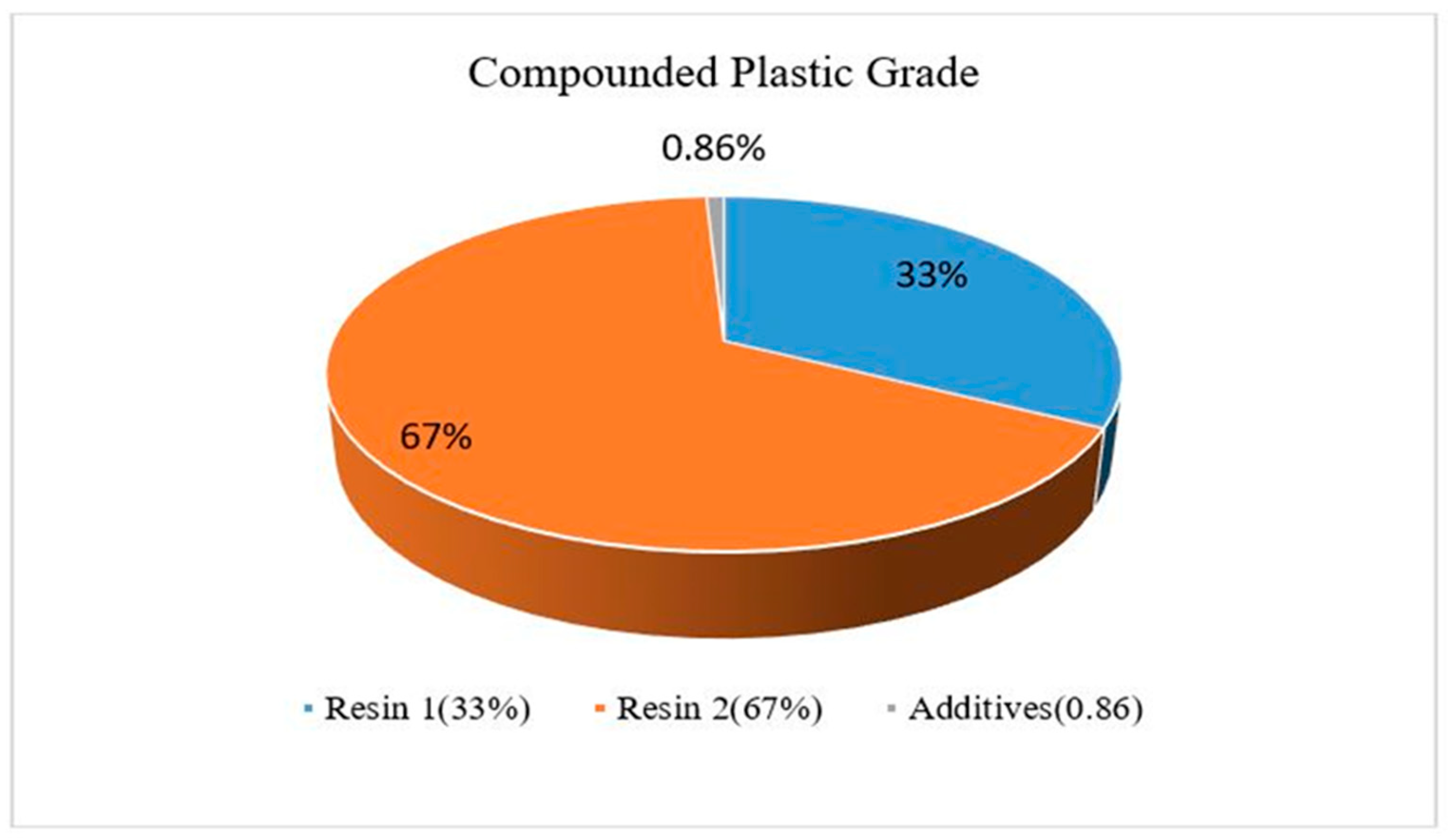
Figure 2.
Schematic diagrams of process methods of plastic.
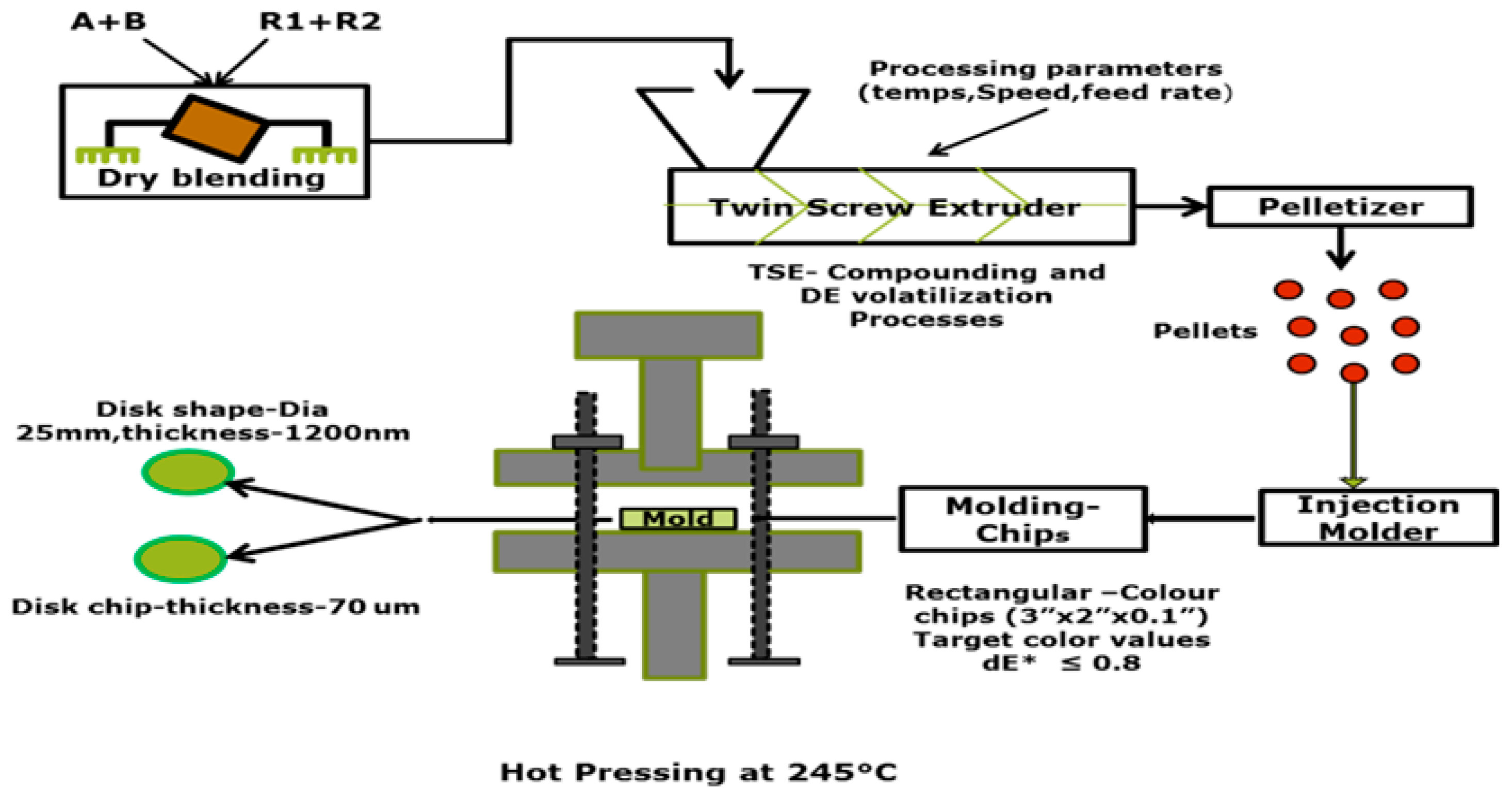
Figure 3.
(a) Three Level Full Factorial Design, (32 runs). (b). Box Behnken Design (17 Runs).
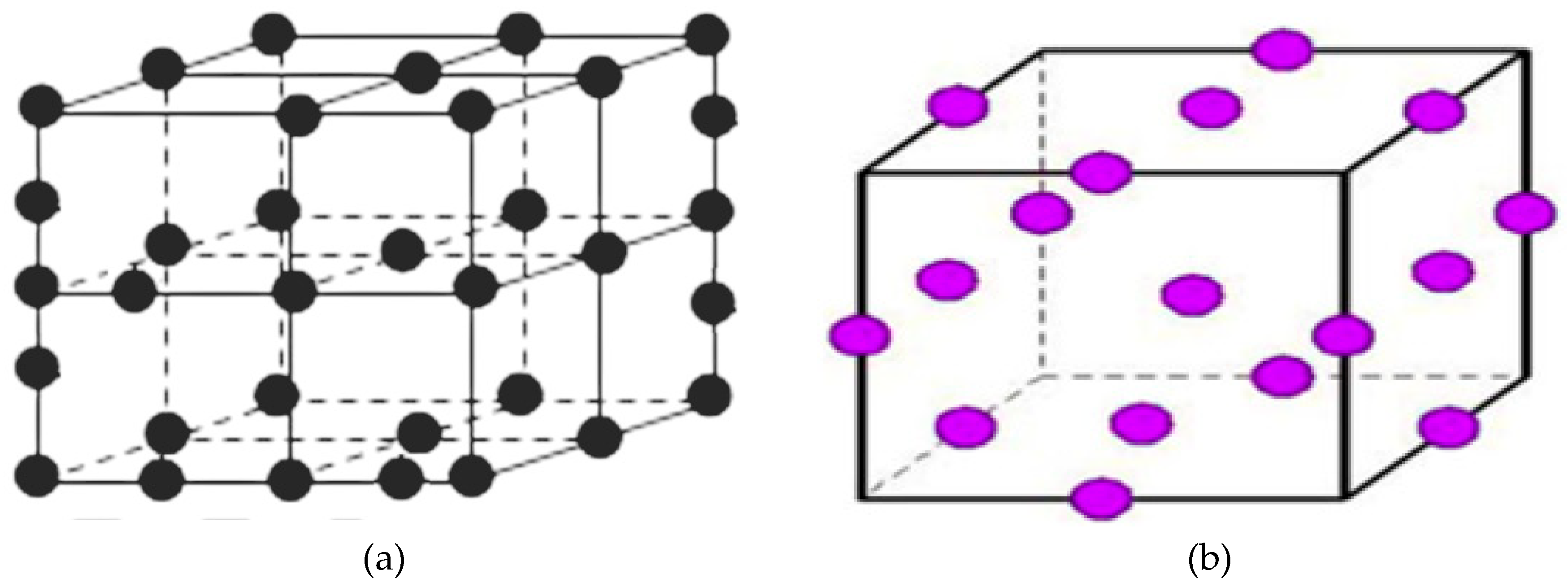
Figure 4.
(a) Interaction Sp & FRate for BBD at (a) 274.23 oC for dL*, (b) 3LFFD at 245.2 oC for dL*.
Figure 4.
(a) Interaction Sp & FRate for BBD at (a) 274.23 oC for dL*, (b) 3LFFD at 245.2 oC for dL*.
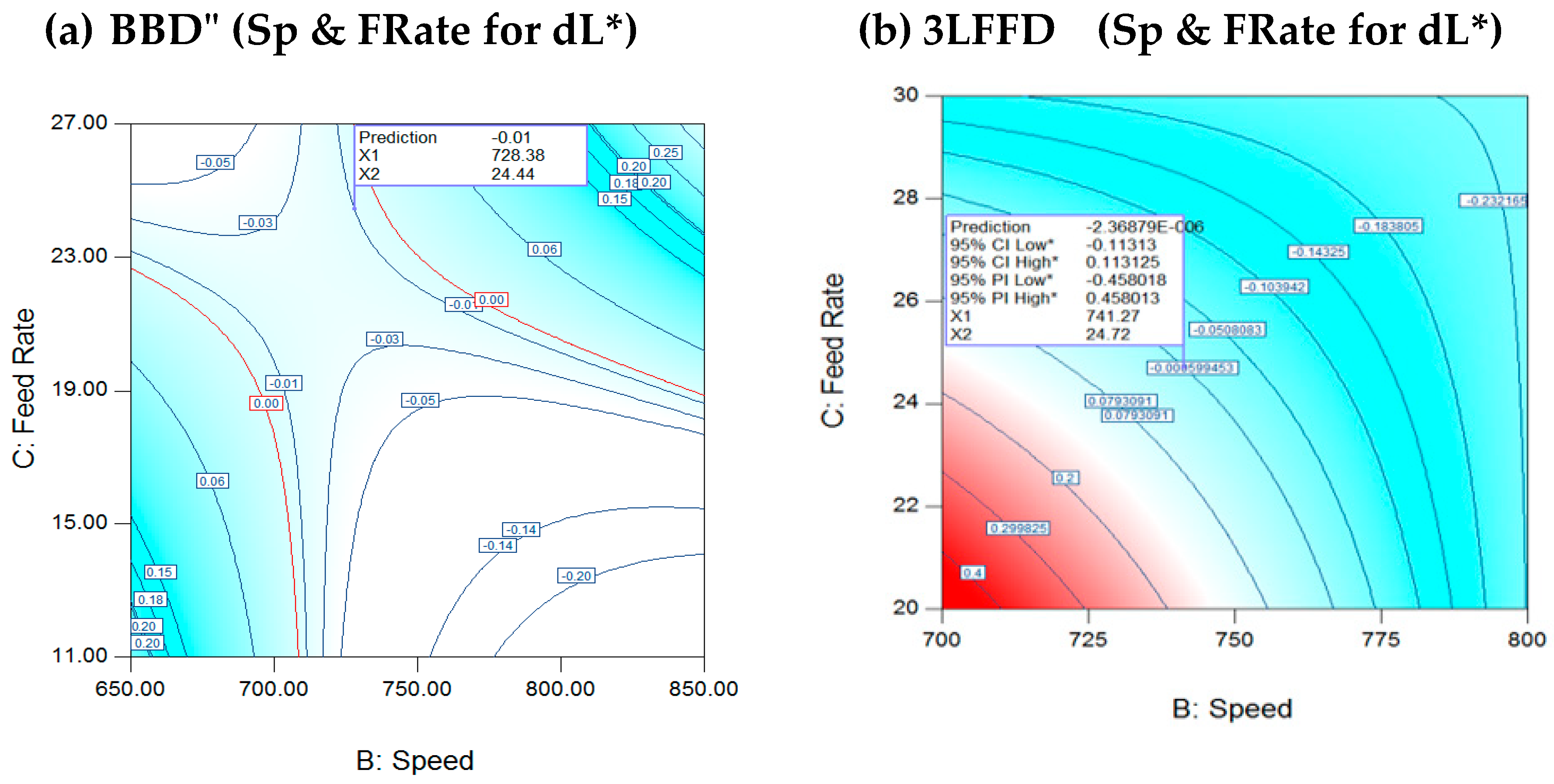
Figure 5.
(a): Interaction Sp & FRate for BBD at 274.23oC for (da*), (b) 3LFFD at 245.2oC for (da*).
Figure 5.
(a): Interaction Sp & FRate for BBD at 274.23oC for (da*), (b) 3LFFD at 245.2oC for (da*).
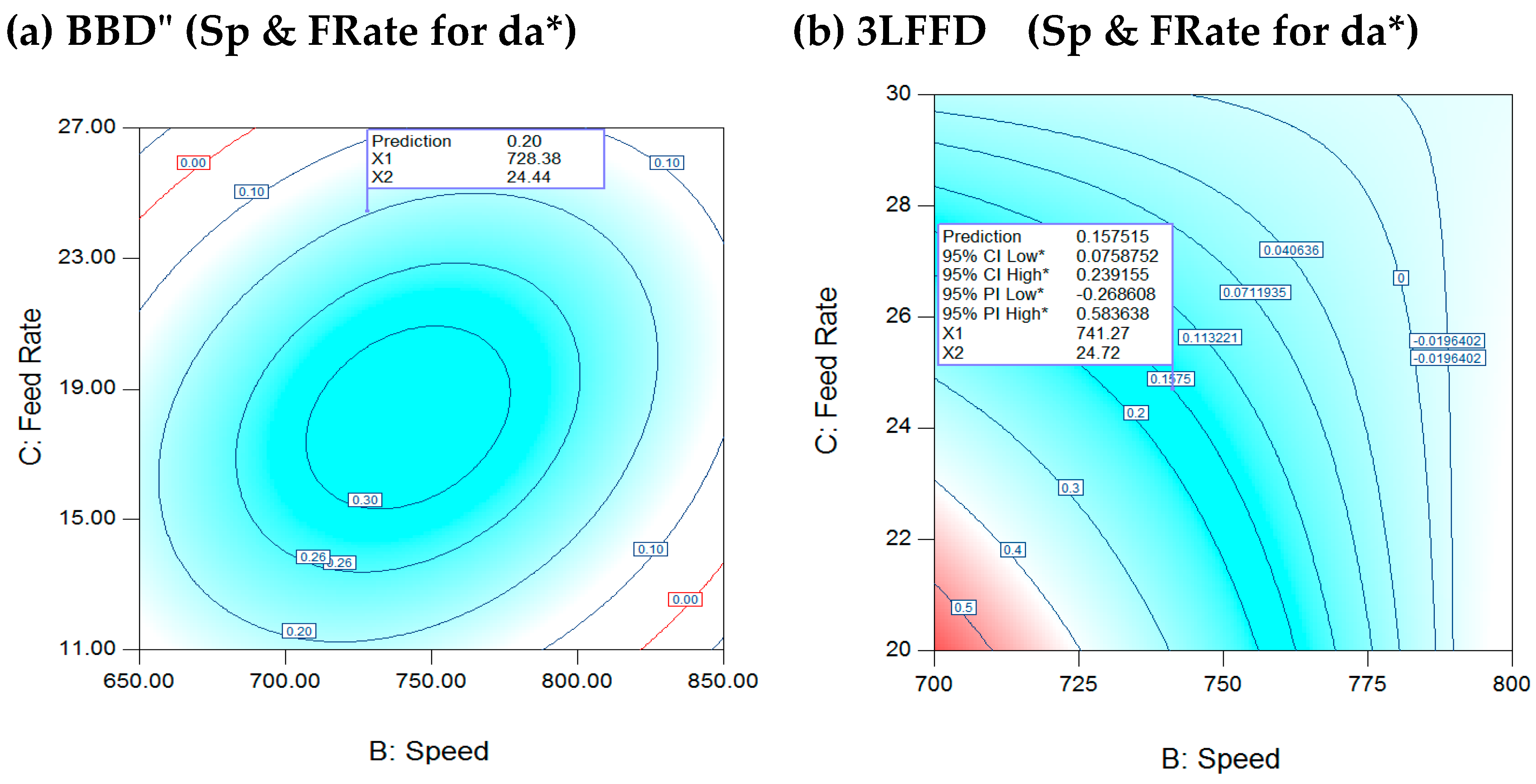
Figure 6.
(a): Interaction Sp & FRate for BBD at 274.4 oC for db*, (b): 3LFFD at 245.2 oC for db*.
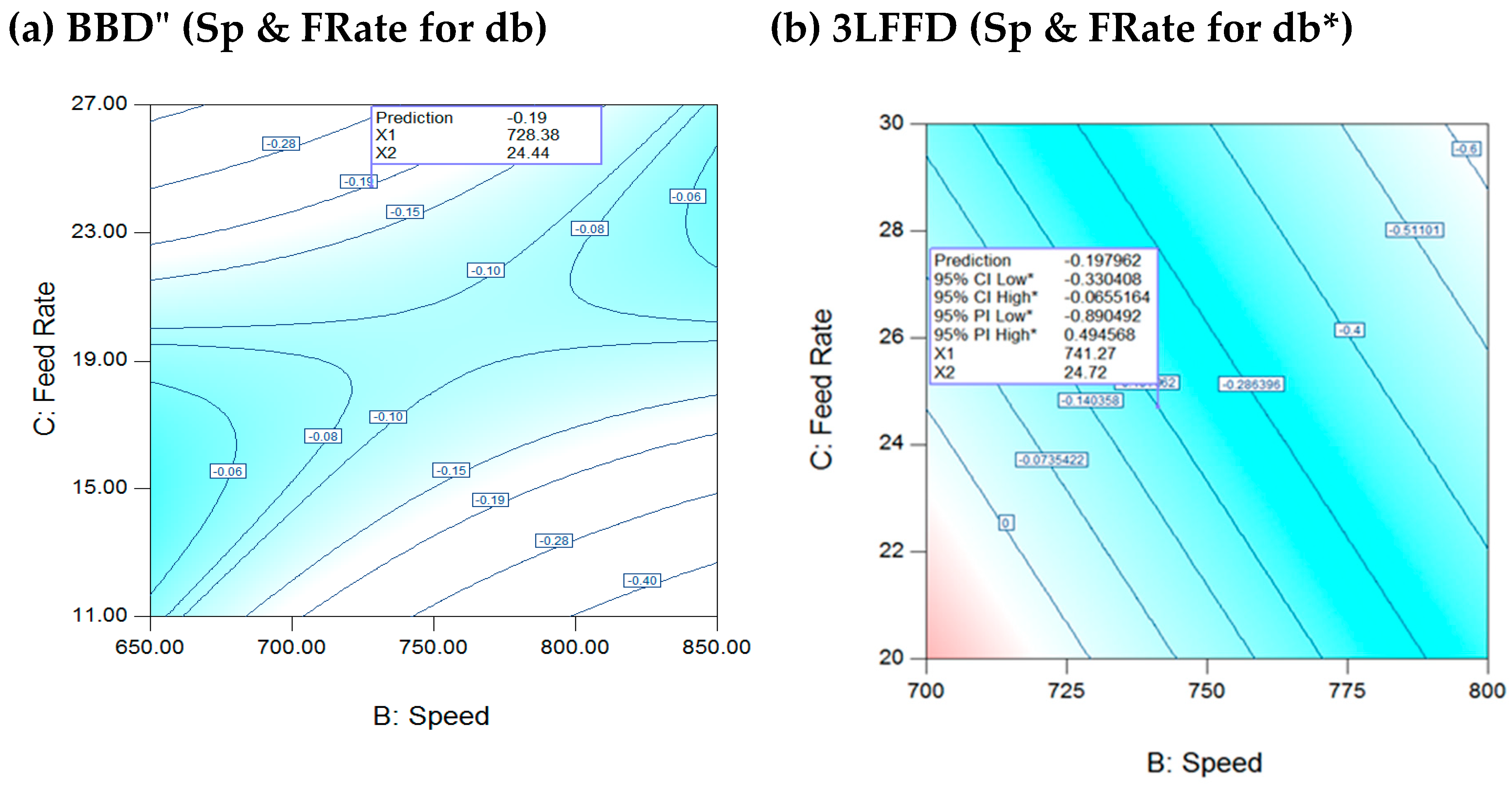
Figure 7.
SME’ plot: (at 274.23oC and 728.38 rpm).
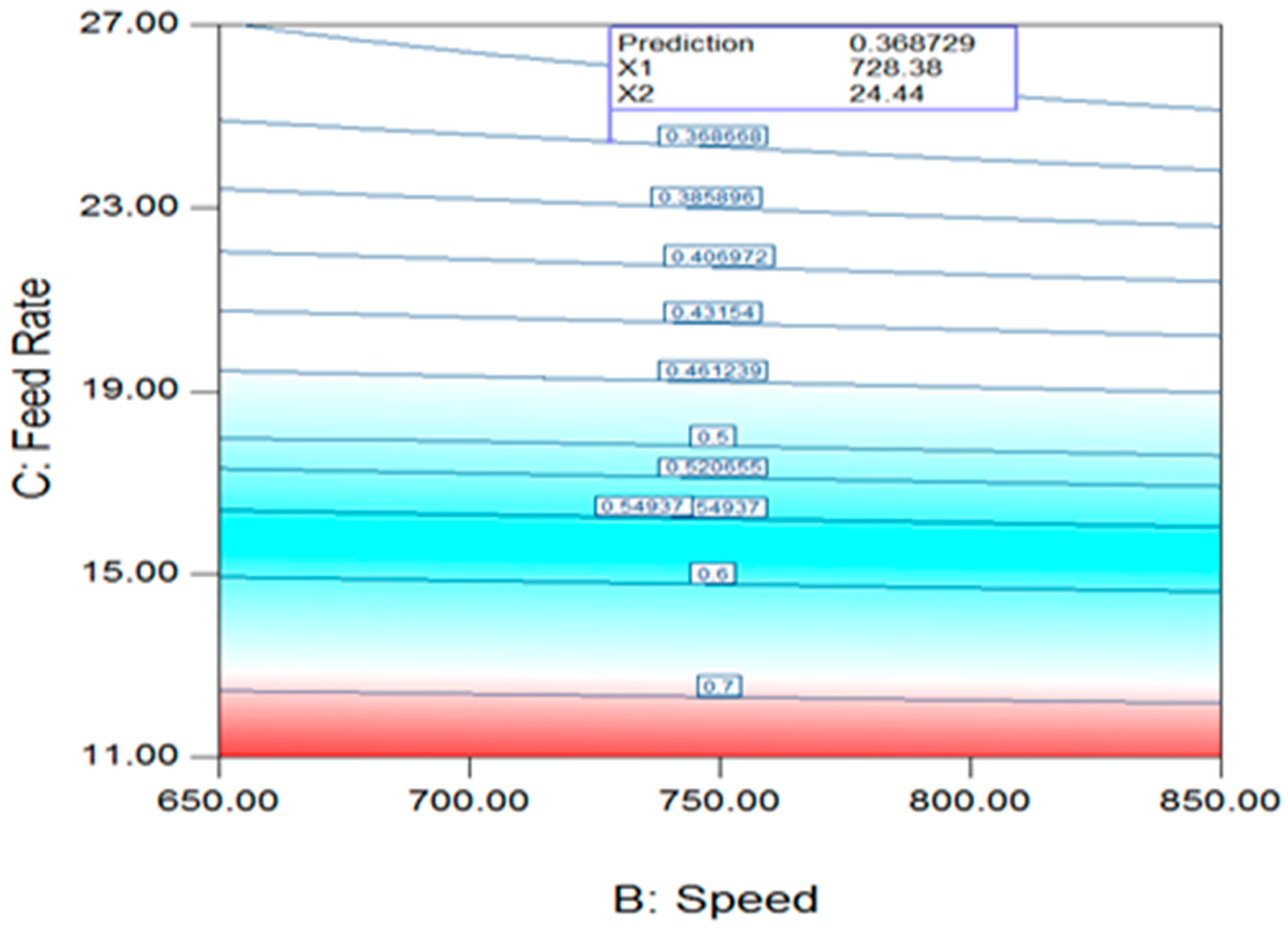
Figure 8.
(a) Desirability at 24.44 kg/hr FRate, (b) Desirability Graph at 245.2 oC Temp. A= T; B= Sp, C= FR.
Figure 8.
(a) Desirability at 24.44 kg/hr FRate, (b) Desirability Graph at 245.2 oC Temp. A= T; B= Sp, C= FR.
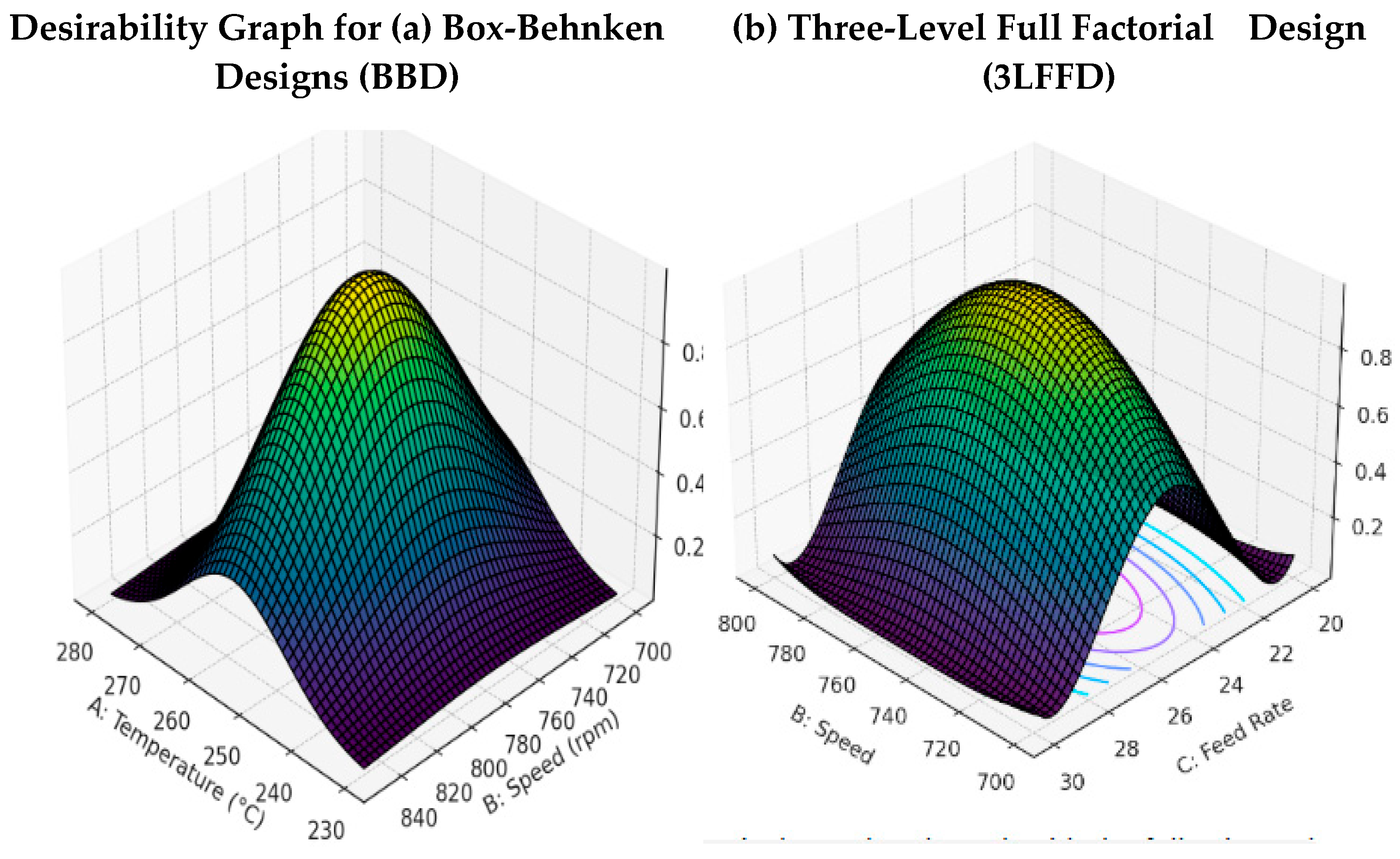
Figure 9.
(a): Temp-speed contour plot (FRate = 24.44 kg/hr), (b): Speed-FRate Contour plot: at (245.2 oC).
Figure 9.
(a): Temp-speed contour plot (FRate = 24.44 kg/hr), (b): Speed-FRate Contour plot: at (245.2 oC).
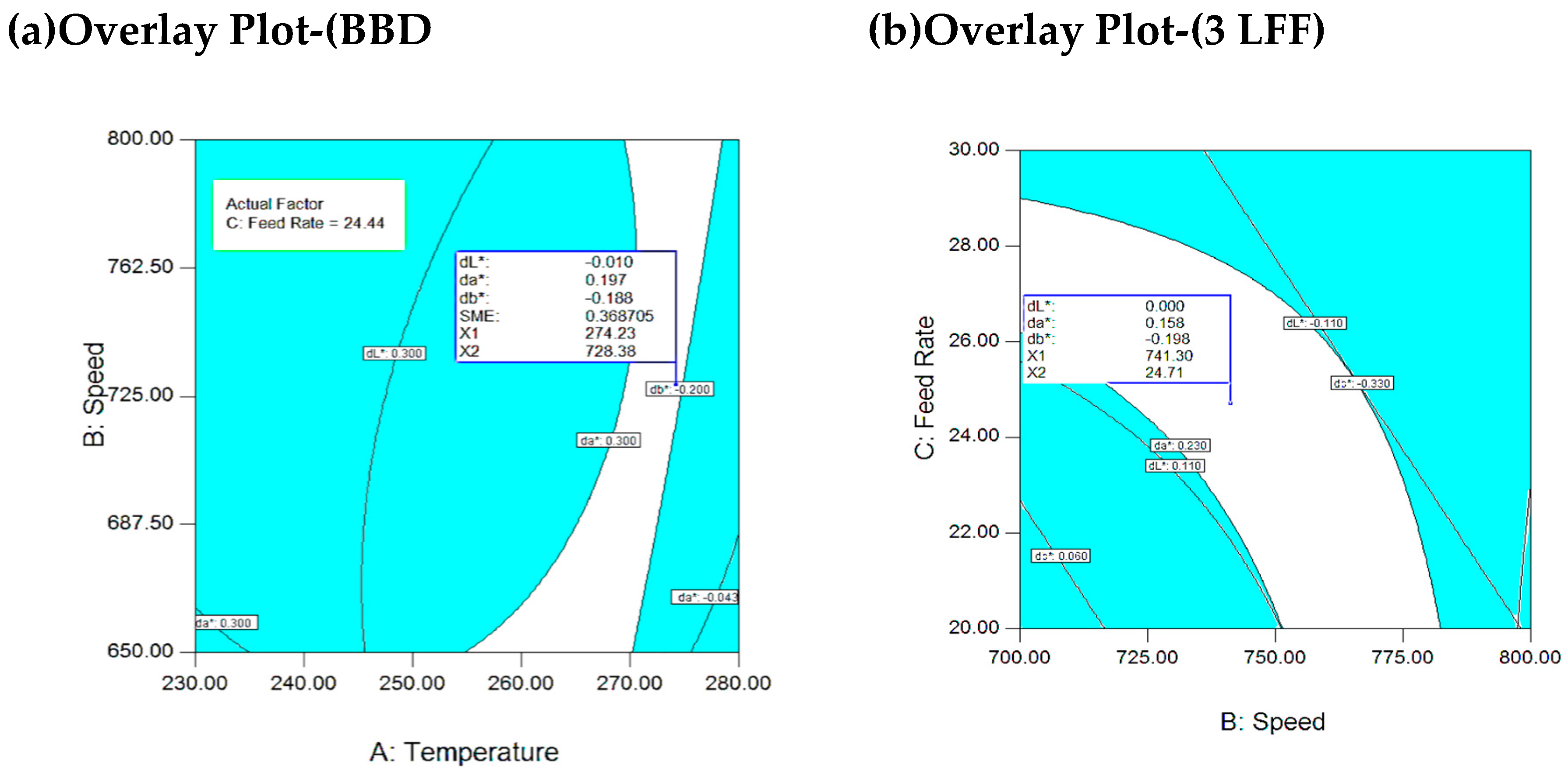
Figure 10.
(a): SEM agglomeration Micrographs for variation of Feedrate; (b): SEM agglomeration Micrographs for variation of Speed.
Figure 10.
(a): SEM agglomeration Micrographs for variation of Feedrate; (b): SEM agglomeration Micrographs for variation of Speed.
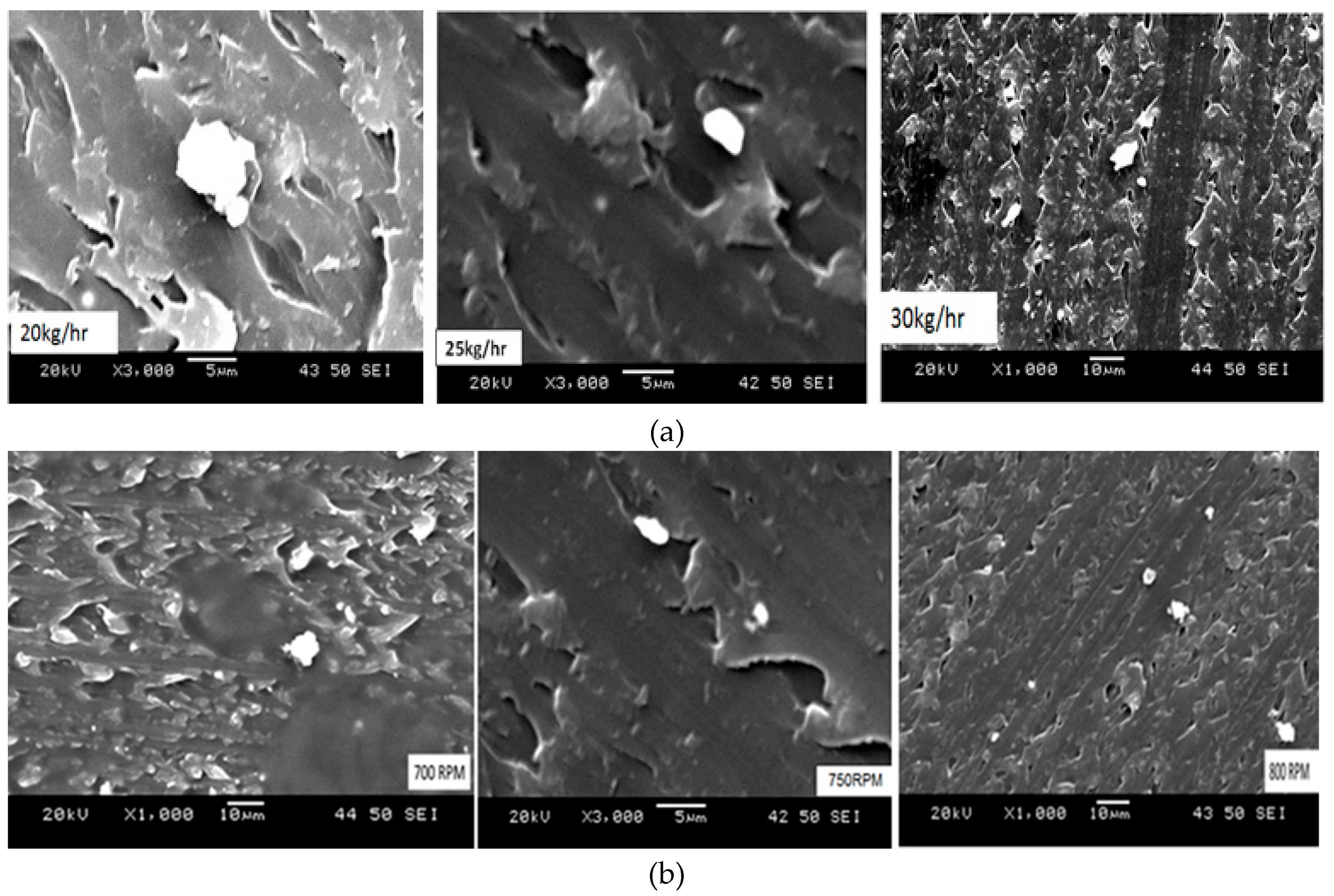
Figure 11.
SEM micrograph of raw pigments - Red, 3000X (Agglomerations’).
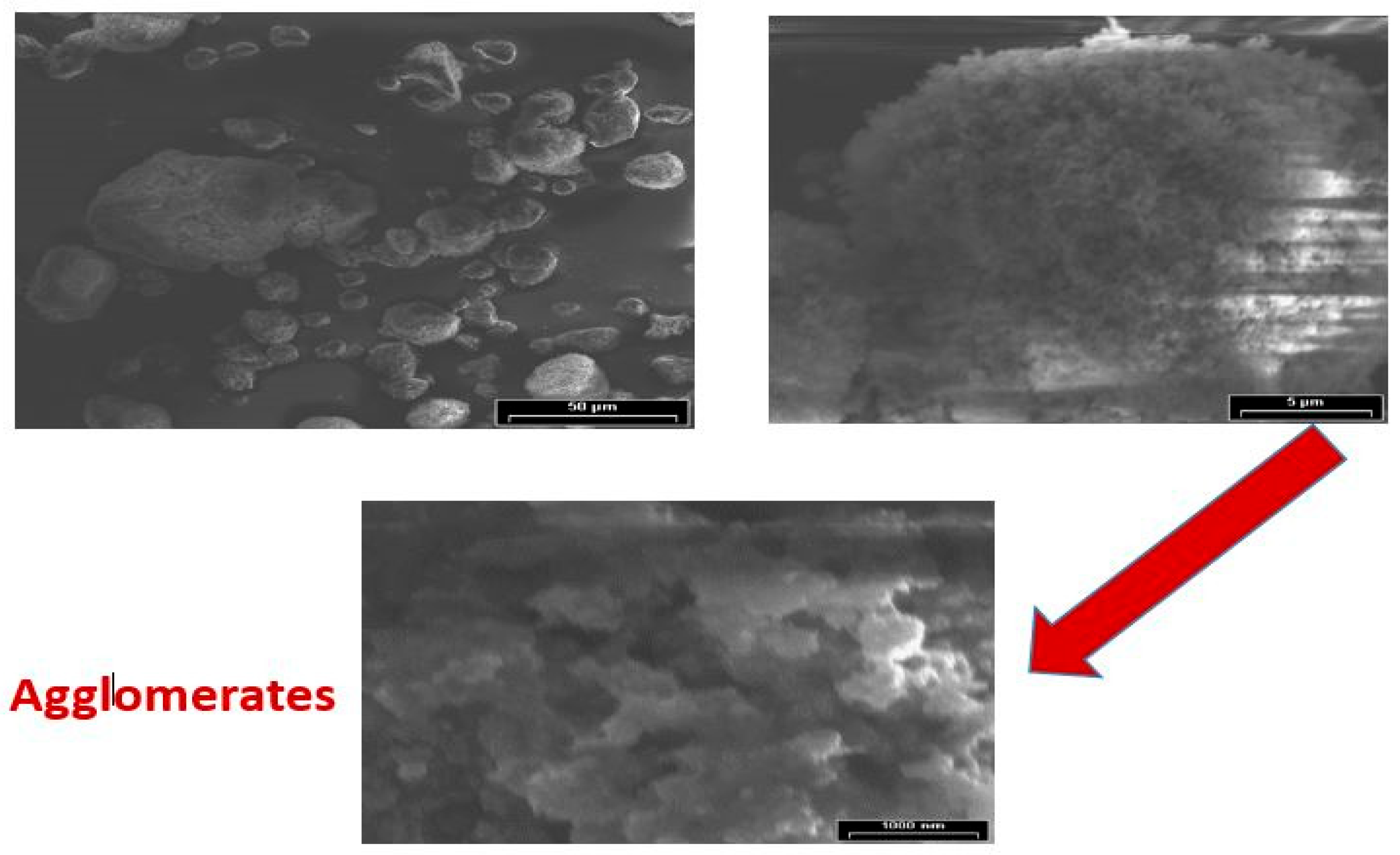
Figure 12.
Micro CT micrographs of PC grade at center point: (a) agglomerations image at 250 X, as well as. (b, c) particle shape (d) pigment distribution,
Figure 12.
Micro CT micrographs of PC grade at center point: (a) agglomerations image at 250 X, as well as. (b, c) particle shape (d) pigment distribution,
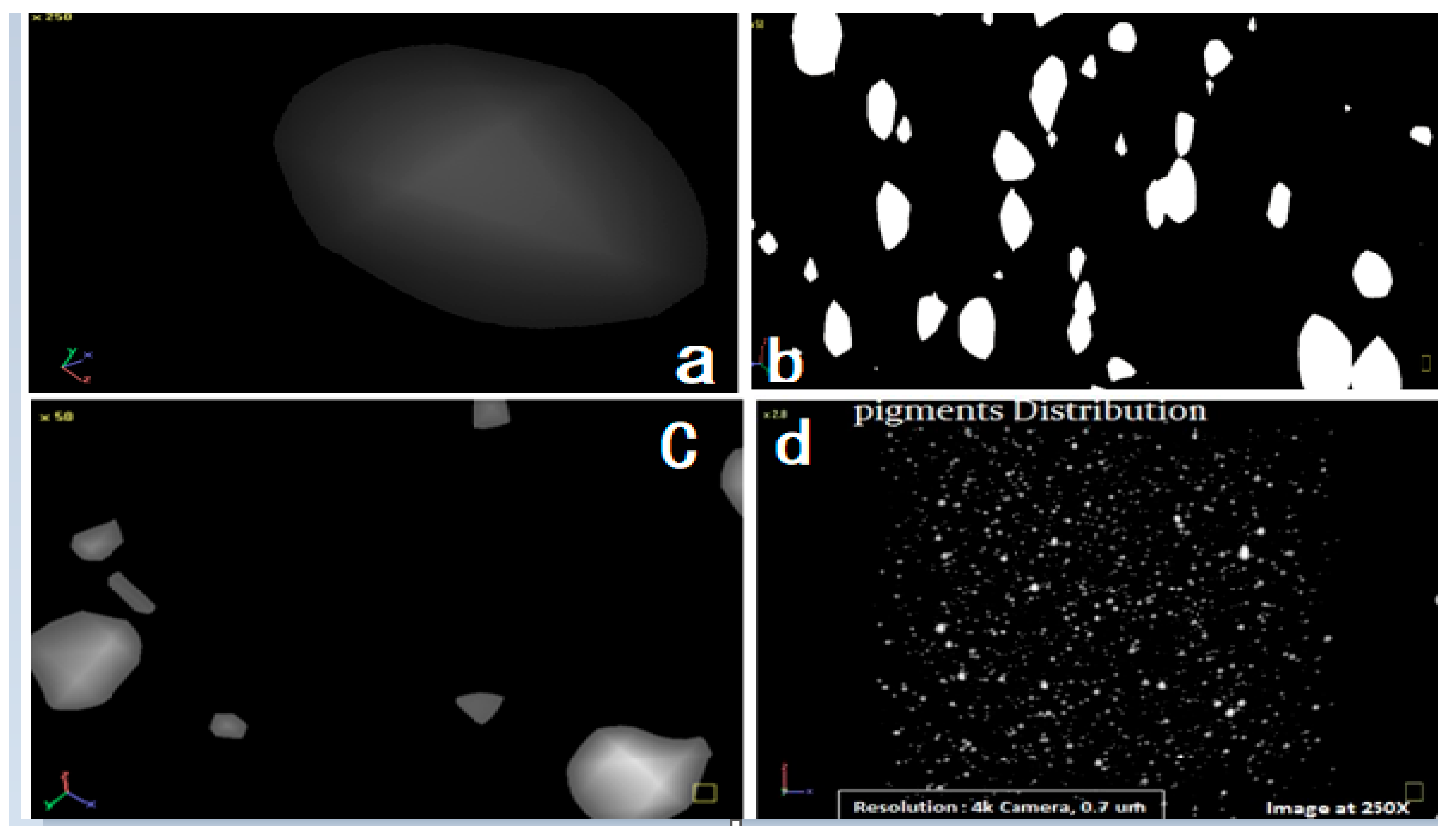
Table 1.
Various pigments & two PC resins / Color formulation.
| (S#) | (Type) | (PPerHundred) |
| #1 | Resin1 | 33.0 |
| #2 | Resin2 | 67.0 |
| #3 | PigmentA | 00.20 |
| #4 | PigmentB | 00.05 |
| #5 | PigmentC | 00.0004 |
| #6 | PigmentD | 00.0016 |
| #7 | PigemntE | 00.0710 |
Table 2.
Experimental design level and parameters for BBD and 3LFFD.
| Design Models | Units | 3 Levels | ||
| -1 | 0 | +1 | ||
| 3LFFD | Temp-°C | 230 | 255 | 280 |
| BBD | 230 | 255 | 280 | |
| 3LFFD | Speed -rpm | 700 | 750 | 800 |
| BBD | 650 | 750 | 850 | |
| 3LFFD | F.Rate-kg/h | 20 | 25 | 30 |
| BBD | 11 | 19 | 27 | |
Table 3.
(ANOVA) Testing the hypothesis that RSM Used with da*, db*, dL*, & SME.
| (Response) | (Significant Terms) | (R2) | (Predicted R2 ) | (Adjacent R2) |
(Adequate Precision) |
|
| BBD | (dL*) | BC, B2 , C, B, A | 0.940 | 0.840 | 0.910 | 17.420 |
| 3LFFD | C, B, A, AB, BC, AC | 0.780 | 0.380 | 0.550 | 0.550 | |
| BBD | (da*) | C, B, A, C2, , B2, A2, AC, BC | 0.980 | 0.890 | 0.970 | 27.80 |
| 3LFFD | C, B, BC | 0.750 | 0.240 | 0.390 | 8.530 | |
| BBD | (db*) | C, B, A, B2, A2, BC | 0.720 | 0.400 | 0.560 | 5.620 |
| 3LFFD | B, C | 0.750 | 0.280 | 0.300 | 8.610 | |
| SME | C, B, A, A2, C2 | 0.990 | 0.970 | 0.930 | 106.0 | |
A= Temperature, B= Speed, C = FRate.
Table 4.
(da*, db*, dL*, & SME) Regression Model.
| (Response) | (Regression Model) | |
| (dL*) | (BBD) | +12.34563 - 0.011717 * T - 0.018803 * Sp - 0.22115 * FRate + 3.09375E-004 * Sp * FRate + 8.38889E-006 * Speed2 |
| (3LFFD) | +63.86390 - 0.19647 * T -0.065085 * Sp - 0.99472 * FRate +1.84353E-004 * T * Sp +1.96624E-003 * T * FRate + 6.39611E-004 * Sp * FRate | |
| (da*) | (BBD) | -34.33712 + 0.20508 * T + 0.024262 * Sp + 0.069289 * FRate - 2.16667E-004 * T * FRate + 1.20833E-004 * Sp * FRate - 4.07867E-004 * T2 - 1.78250E-005 * Sp2 - 2.74609E-003 * FRate2 |
| (3LFFD) | +14.59778 - 0.018496 * Sp - 0.47296 * FRate + 5.98224E-004 * Sp * FRate | |
| (db*) | (BBD) | -19.24168 + 0.18004 * T -5.00208E-003* Sp - 0.077943 * FRate + 2.52083E-004 * Sp * FRate-3.66316E-004 * T2 - 2.86116E-003 * FRate2 |
| (3LFFD) | +4.08697 - 4.78866E -003 * Sp - 0.029746 * FRate | |
| (SME) | +2.72593 - 9.00716E-003 * T - 6.00329E-005 * Sp -0.077916 * FRate + 1.64940E-005 * T2 + 1.37360E-003 * FRate2 | |
Table 7.
Optimized Processing Parameters and Corresponding Desirable Color Outputs.
| Design Methodology | Significant Processing Parameters | Optimized Parameters | Number of Runs |
Desirability | Color output dE* | ||||
| dL* | da* | db* | Temp | Speed | FRate | % | |||
| 0C-A | rpm-B | Kg/hr-C | |||||||
| BBD | A,C,BC, B2 | B2 A2 C2 , AC, A, BC | BC, A, A2 C2 | 274 | 728 | 24.4 | 17 | 87 | 0.26 |
| 3 LEVEL | C, B, A, AB, BC, AC | BC, B, C | B, A | 255.7 | 734 | 24.4 |
32 |
77 | 0.25 |
| Core differences | B | BC | BC | 18.3 | 6 | 0.0 | 15 | 10 | 0.01 |
A= Temperature, B= Speed, C = Feed rate.
Disclaimer/Publisher’s Note: The statements, opinions and data contained in all publications are solely those of the individual author(s) and contributor(s) and not of MDPI and/or the editor(s). MDPI and/or the editor(s) disclaim responsibility for any injury to people or property resulting from any ideas, methods, instructions or products referred to in the content. |
© 2025 by the authors. Licensee MDPI, Basel, Switzerland. This article is an open access article distributed under the terms and conditions of the Creative Commons Attribution (CC BY) license (http://creativecommons.org/licenses/by/4.0/).
Copyright: This open access article is published under a Creative Commons CC BY 4.0 license, which permit the free download, distribution, and reuse, provided that the author and preprint are cited in any reuse.


