Submitted:
02 April 2025
Posted:
03 April 2025
You are already at the latest version
Abstract
A single paragraph of about 200 words maximum. For research articles, abstracts should give a pertinent overview of the work. We strongly encourage authors to use the following style of structured abstracts, but without headings: (1) Background: Place the question addressed in a broad context and highlight the purpose of the study; (2) Methods: briefly describe the main methods or treatments applied; (3) Results: summarize the article’s main findings; (4) Conclusions: indicate the main conclusions or interpretations. The abstract should be an objective representation of the article and it must not contain results that are not presented and substantiated in the main text and should not exaggerate the main conclusions.
Keywords:
bathymetry
; topographic survey
; coastal relief
; hydraulic structures
; interpolation
; measurement accuracy
; 3D-modeling
; hydrogeology
; Karatomar reservoir
; Tobol River
; Ayat River
; siltation
1. Introduction
Hydraulic structures and the reservoirs they create play an important role in the global water cycle, regulating the flow of water from the environment into man-made systems. For example, about 57% of the seasonal variability of global surface freshwater (GSW) is compensated by reservoirs [1].
As a rule, after the introduction of regular bathymetry and the study of the bottom morphology of large reservoirs subject to gradual siltation, unjustifiably little attention is paid. Usually, studies and descriptions of reservoirs are limited only to the type, shape, elevation, bed size and the design volume of water in them. At the same time, effective monitoring of the state of reservoirs is necessary for a wide range of practical economic tasks, such as flood modeling and forecasting, calculating the actual useful capacity, including dead volume, planning irrigation and man-made loads and long-term consequences of these structures for the global climate [2,3].
After a series of floods in the spring of 2024 in Kazakhstan, monitoring the state of water resources and, especially, the actual state of hydraulic structures of reservoirs has been made a priority task and is carried out at the state level [4].
For an effective understanding of the ongoing processes and reservoir management, bathymetric studies (obtaining the bottom relief) and coastline relief studies play a key role. Thus, an accurate assessment of the “water level - area - volume” relationships for reservoirs is important for effective hydrological modeling, monitoring the state of reservoirs and forecasting possible seasonal fluctuations in river levels. The main characteristics of reservoir modeling and the relationships between these parameters are derived from the digital model based on the results of its bathymetry [5]. Modern bathymetry methods offer various computerized methods for collecting a large array of primary data, ranging from field test data collection to satellite altimetry.
Manual methods of depth measurement are currently practically not used due to the low accuracy of the digital models obtained on their basis and the significant time costs of personnel to obtain depth data.
Automated bathymetry methods, also based on field work on water bodies, are built on the use of such tools as single- and multi-beam sonars, depth gauges and LiDAR sensors (Bandini, et al., 2018). The methods provide high measurement accuracy, but also require significant time to obtain the required volume of data during field work. In the pool of satellite remote sensing methods for capturing the topography of a water body basin, satellite altimetry [1,6], the Shuttle Radar Topography Mission (SRTM) method based on the use of interferometric synthetic aperture radar [7] and the method based on the use of spaceborne thermal emission and reflection radiometers (ASTER), which relies on pairs of stereoscopic images [8] have recently been singled out.
However, these remote methods also have certain limitations. These limitations are especially significant when it comes to capturing the surfaces of underwater relief of reservoirs [9].
This fact makes remote sensing methods of little use for calculating the actual volume of reservoirs. Given these challenges, accurate bathymetric data are currently still obtained through more tedious on-site fieldwork using tools such as sonars and LiDAR sensors [10].
All used digital water body models are built on deterministic and geostatic interpolation methods [11]. Recently, in contrast to the previously dominant methods of mathematical one-dimensional interpolation, multidimensional interpolation methods and interpolation methods based on the use of artificial intelligence apparatus are increasingly being used [12].
First, when using interpolating algorithms, interpolation on a regular [13] and irregular data grid [14] is distinguished [15]. The latter, although more strict to the interpolation apparatus, are still less demanding to the array of initial data. This allows in the process of research to transfer part of the complexity from field work to the office post-processing of data when modeling the object under study, which is still more convenient.
Deterministic interpolation methods generate surfaces from discrete measurement values (data point arrays) based either on the degree of similarity (inverse distance weighted methods) or, for example, the level of smoothing (radial basis functions) [16]. Geostatistical interpolation methods (variations of kriging algorithms and the like) [17] exploit the statistical properties of the measured points. Geostatistical methods are more flexible with respect to the input data, but within a family of methods, such as kriging, different requirements are put forward for the conditions to be met for the output results to be acceptable. Disjunctive kriging and empirical Bayesian kriging generally yield lower absolute interpolation errors for water bodies than universal kriging and simple kriging [17,18]. However, [19] [20] note in their studies that deterministic radial basis function interpolation is comparable to kriging in both accuracy and performance in some cases.
Interpolation methods based on artificial intelligence apparatus are often reduced to neural network methods [21,22] (multilayer perceptron (MLP) [23,24], again but already a radial basis function neural network (RBFN) [25], back propagation network (FNN) [26], deep neural network (DNN) [27] and recently have been investigating the applicability of capsule neural networks (CapsNet)) [28].
The authors' work addresses three main research questions:
- First, what is the real state of the Karatomar Reservoir after 78 years of operation;
- Second, how accurately does the bathymetric study convey the reservoir relief after interpolation of bathymetric data?
- Third, with what step of drone tacks should the bathymetric survey of the basins of flat reservoirs be carried out to achieve the required accuracy of 3D modeling?
To solve the tasks, the analysis was carried out based on the materials of the bathymetric survey of the regulated volume of the Karatomar Reservoir over an area of 61 km2 carried out in July-August 2024 by a team of authors and a detailed additional survey of the reservoir bay with the construction of corresponding digital elevation models. The bottom relief of the reservoir is represented by flat areas of a flooded accumulative plain with predominant slopes of about 0.5–0.8 o/oo, dissected by the river beds of the Tobol and Ayat rivers.
The transformation of the reservoir bottom relief compared to the design is due to the processes of bottom erosion in the flow zones (meander) and gradual silting of stagnant areas.
The accuracy of interpolation and modeling with different frequencies of bathymetric boat tacks was assessed. Based on the modeling results, an analysis of the accuracy of the obtained reservoir modeling results was carried out.
The approach proposed by the authors is a reliable solution for the first stage of the study for an accurate assessment of the current bathymetry of the reservoir and establishes more reliable values of the “water level – area – volume” ratio using the example of the Karatomar reservoir of the Republic of Kazakhstan with the possibility of replicating the results for any lowland reservoirs.
2. Materials and Methods
The object of the study was the Karatomar Reservoir, located in the Kostanay region of the Republic of Kazakhstan. The reservoir was built at the confluence of the Tobol and Ayat rivers. Bathymetric measurements at the research site were carried out in July-August 2024.
Bathymetric studies were carried out using an Apache 3 autonomous drone with a single-beam single-frequency echo sounder. The technical characteristics of the drone and echo sounder are given in Table 1.
To adjust the accuracy of the drone echo sounder, the echo sounder corrections were determined on the waters of the bay of the Karatomar reservoir using the calibration method. The work was performed using a calibration disk and a hydrometric rod. Accuracy adjustment was made by setting the parameters at depths of 1, 3 and 5 meters of this reservoir (bay of the reservoir), plus an additional 10 and 15 meters for the reservoir itself.
The drone sonar passed state verification in 2024.
To obtain maximum accuracy of primary data and increase the efficiency of using the drone, georeferencing was carried out using DGPS. The CNCNAV GPSS station was used. The station received a certificate of conformity from the Republic of Kazakhstan.
The drone run routes were constructed in the AutoPlanner 2.0.11.9341 software product. The WGS84 coordinate system was used. Pre-processing of the obtained bathymetric data was performed in the freely distributed GIS package QGis v 3.34.11. In this package, sections were obtained and a digital model of the reservoir bowl was processed. The water edge was constructed using the superimposed Sentinel-2_L2A_True_color image from 04/07/2024, corresponding to 98% of the reservoir bowl being full (according to data from the Kazvodkhoz Foundation). A comparison of the quality of available space images from 14/06/2024 and 04/07/2024 with a resolution of 30 m/pixel is given below. The quality of the images is determined by the cloudiness on the day of the space survey above the research object. The image from 04/07/2024 has the best quality indicators (Fig. 1).
The decrease in the area of the water zone in the Sentinel-2_L2A NDWI (Normalized Difference Water Index) image over the Google and Sentinel-2_L2A_True_color images is caused by significant overgrowing of the riverbed with reeds within the boundaries of the beginning of the reservoir (despite the maximum level of water rise in the reservoir over the past 10 years).
The length of the water edge line was 93.77 km, which, with a photo resolution of 30 m/pixel, corresponds to a generated error in delineating the reservoir surface area of no more than 5.63 km2.
Interpolation by initial data and modeling of the surface of the reservoir bowl and the bay were performed in the Surfe software product. The geostatic method of simple crying was chosen as the interpolation algorithm.
3. Results
3.1. Analysis of Potential Methods for Studying Reservoir Bowls
In order to understand the capabilities of various survey methods within the framework of the task, an analysis of various modern methods of digital modeling of the underwater topography of reservoirs was carried out (Table 2).
Manual methods such as compass survey and visual survey in topographic methods were not considered by the authors due to the fact that at present (like most manual methods) they are gradually falling out of use [29].
Initial attempts to determine the underwater topography of water bodies using remote sensing methods were based on the methods of [30,31,32,33]. The issues of modern successful remote sensing for assessing the bathymetry of reservoirs are systematized in the works [6,8,9,34].
Systematizing the results of the analysis of space remote methods, we can say that the existing methods for assessing the state of reservoirs can be conditionally represented as two large groups [35,36]. The first category combines satellite image processing methods
to track changes in the water surface area of an object using radar altimetry. This group is highly accurate methods, but their applicability is limited due to the inability to scan the underwater relief.
The second group of methods is based on an attempt to reconstruct the bathymetry of the reservoir [5,38], which allows estimating the full relief of the object. However, this group of methods often relies on overly simplified assumptions for bathymetric reconstruction, which leads to a decrease in accuracy in the conditions of complex reservoir relief [36].
The methodology issues of "gluing" interpolation data of underwater and coastal relief when constructing digital maps of water bodies are considered [43] [44].
The key point in constructing 3D models adequate to the tasks remains the choice of interpolation methods optimal for a given reservoir and data set and the determination of the minimum sufficient number of points of this initial data. The use of overly simplified approaches for interpolation can negate the results of the studies due to a significant loss of accuracy.
One of the most important problems of geodetic research when studying a water body using bathymetry data [15,29] is determining the purpose of developing an interpolation model.
Deterministic interpolation and geostatistical analysis tools offer a variety of different interpolation methods, each with its own unique features and often providing significantly different results.
First, all methods used in geodata interpolation can be divided into exact (ORB, RBF) and inexact - most often stochastic (LPI, KSB, Kriging). In exact rigid methods, at each output position, the interpolated surface will have exactly the same value as the value of the input data, while some are non-rigid, with the possibility of deviating the interpolated value from the value determined at a given point [45]. It should also be taken into account that for some decisions it is important to consider not only the interpolated values, but also the uncertainty (variability) associated with this interpolation [46].
Interpolation methods also differ in terms of complexity, which can be measured by the number of assumptions that must be satisfied to validate the model, and in terms of computational complexity, which is characterized by the volume of mathematical transformations and elementary machine operations.
In connection with the conducted analysis for interpolation of bathymetric data of the reservoir, in our opinion, the method of linear interpolation and kriging (more precisely, the method of simple kriging) is of interest, as, firstly, it provides the required smoothness of the interpolated relief, typical for slowly flowing flat rivers, secondly, the possibility of taking into account potential noise and missing data, and, thirdly, it has acceptable parameters of computational complexity (the maximum time of bathymetric calculations on a computer based on an Intel i7-13700K processor with 8 GB RAM did not exceed 30 minutes).
3.2. Analysis of Hydrogeology of the Tobol and Ayat Rivers in the Karatomar Reservoir Zone
The Karatomar reservoir is located at 52°53′40″N 63°01′45″E in Kazakhstan, in the Beimbet-Mailin district of the Kostanay region. The need for a large reservoir in this area was due to the development of the Sokolov, Sarbay, Kachar iron ore deposits and the need to provide water to the cities of Rudny and Kachar under construction.
The reservoir is located in the valley between the Trans-Ural and Turgay plateaus. It was formed by a dam built in 1966 and filled with water in 1967–1969.
The reservoir was built on the Tobol River, and the Ayat River flows into the reservoir from the west. A valley-type reservoir with the following planned parameters: area 88.0–93.7 km2, total volume 791 million m³, useful volume – 562 million m³, length – 72 km, width – 4 km, depth up to 19.8 m, water discharge for river flooding 1.3 m3/s. In 2024, when the reservoir was 99% full during the spring flood due to melting snow, the emergency discharge of the reservoir exceeded 3250 m3/s. The catchment area of the reservoir is 28.5 thousand km2, the length of the coastline is 102 km. A large tributary is the Ayat River. The reservoir was built using the long-term flow regulation type. Intra-annual fluctuations in water level reach 11 m. Water mineralization is 200–400 mg/l, the waters belong to the sodium hydrocarbonate type. The operating mode of the Karatomar reservoir (Fig. 2) is intermediate-flow, as it is controlled by the volume of filling and discharge from the Verkhnetobol reservoir.
The reservoir is an additional flow regulator and a reserve reservoir for replenishing the downstream flow reservoirs, as well as a source of drinking water supply for a number of settlements connected to the Kostanay water pipeline. In addition to water supply for settlements, water is used for irrigation of agricultural lands and fisheries.
Water exchange in the Karatomar reservoir is more active than in the Verkhnetobol reservoir due to the constant inflow of relatively fresh water from the Ayat River and constant discharge for flooding the Tobol River and replenishment of the downstream Sergeev and Amangeldy reservoirs. Filling of the reservoirs is carried out mainly in the spring months: April, May, due to the runoff of the spring flood.
The accumulative type of the reservoir relief was represented by gently sloping and horizontally stepped surfaces of terraced plains, the morphological expression of which is very weak. By genesis, the accumulative plain is alluvial and is found along rivers.
The Tobol River flows through the territory of Kazakhstan and Russia, is the left and most abundant tributary of the Irtysh River. The length of the river is 1591 km, the area of the drainage basin is 426,000 km². The difference in altitude between the source and the mouth is 237 m. The location of the Karatomar Reservoir under study is 1257 km of the Tobol River (the confluence with the Ayat River). The Tobol is formed at the confluence of the Bozbie River with the Kokpektysay River on the border of the eastern spurs of the Southern Urals and the Turgai tableland of the country (51°28′00″N 61°00′31″E). The middle and lower reaches of the river are within the West Siberian Plain in a wide valley with a winding channel. The right bank rises above the left, as the Tobol flows over a deep fault in the earth's crust and separates the Kurgan synclinorium and the Tobol-Ubagan uplift.
The relative height of the floodplain terraces above the water level increases downstream from 12-15 m in the area of the Karatomar reservoir to 35 m north of the city of Kostanay.
The maximum width of the floodplain terrace in the area of the reservoir reaches several kilometers. This terrace is separated from the floodplain surface by a sharply expressed ledge.
The river bed in the area of the studied reservoir is located in a wide floodplain, composed of modern sandy deposits. The width of the channel from 10 to 50-100 m, the depth is 4-8 m. The current in low water is 0.1 m/s, in flood up to 3 m/s, the slope is 0.0003. The left bank of the river is often steep. The riverbed is winding with meanders and oxbow lakes that are flooded only during floods, almost everywhere surrounded by willow and reed thickets. The river flow is regulated by reservoirs. The river is fed mainly by snow, while downstream the share of rain increases. The flood occurs from the first half of April to mid-June in the upper reaches and until the beginning of August in the lower reaches. The average annual water flow is 26.2 m³/s in the upper reaches (898 km from the mouth), 805 m³/s at the mouth (maximum 348 m³/s and 6350 m³/s, respectively). Average turbidity is 260 g/m³, annual sediment runoff is 1,600 thousand tons. It freezes in the lower reaches in late October - November, in the upper reaches in November, opens up in the second half of April - the first half of May.
As a result of the above, it can be said that the hydrogeology of the Tobol River includes the following aspects:
- the hydromorphological picture is represented by alternating shallow riffles with shallow and medium-depth pools. The depth of the pools can reach up to 5 meters, and in some cases up to 10 meters or more;
- the river bottom is sandy-silty, rocky in places;
- the width of the channel varies from 50 to 400 meters;
- the banks are mainly loamy, overgrown with small bushes, slightly intersected by dry stream beds. The banks are steep, in places precipitous, 5-6 meters high, and at the confluence with the slopes of the valley they reach up to 30 meters;
- snow waters are predominant in the river's nutrition (70-90%). In winter, rivers are fed by underground waters, in summer - by underground waters, less often by rain;
- the water regime is characterized by a pronounced spring flood (up to 85-96% of the annual flow) and a long low water period;
- the mineralization of water during the spring flood period is 100-200 mg/l, and the hardness is 0.5-1.25 millimoles/l. In summer, the mineralization of water increases, the water becomes sulfate or weakly hydrocarbonate.
Ayat is a river in Russia and Kazakhstan, flowing through the Varna district of the Chelyabinsk region of Russia (22 kilometers from the source) and the Taranovsky, Fyodorovsky Kostanay districts of the Kostanay region of Kazakhstan (95 km). Ayat is formed by the confluence of the Karataly-Ayat and Archagli-Ayat rivers. The river flows into the Tobol River in the area of the Karatomar reservoir. The length of the river is 117 km, the area of the drainage basin is 13,300 km².
Geomorphological features of the Ayat River:
- the soils of the basin are mainly sandy and loamy, sometimes salty. Alluvial channels is located in a well defined river valley;
- the channel is gently winding, stretching, located in a well-defined river valley;
- the bottom of the river is sandy-silty, rocky in places;
- the width of the riverbed varies from 5 to 20 meters;
- the maximum water depth is 2 meters;
- the water regime is unstable, almost the entire annual flow occurs during the spring flood;
- due to large fluctuations in the water level, there are spits, islands-middens, and shoals on the river.
A significant part of the Ayat River basin is formed by 383 endorheic lakes (total area 208 km²). During the observation period, the river froze to the bottom 5 times in winter.
3.3. Evaluation of the Boat's Tack Pitch to Ensure the Required Measurement Accuracy
When conducting a reservoir study using the instrumental bathymetry method, the issue of choosing the measurement pitch (in the case of hydroacoustic measurements - the boat's tack pitch for taking points) is important for achieving the required accuracy. In terms of the measurement pitch on the course, such a task does not arise, since the boat's equipment made it possible to obtain points with excess density - more than 10 points per meter of the distance traveled). Due to rather difficult hydrometeorological conditions at the start of the research (July 2024 was characterized by average wind speeds from 13 to 25 m/s or from 6 to 8 points on the Beaufort scale [47], it was decided to carry out an initial assessment of the necessary step of the tacks of the bathymetric boat runs to ensure the accuracy of the measurements on the bay of the reservoir (more precisely, at the mouth of the channel of a seasonally drying up stream flowing into the reservoir and called the "bay" by the local population). The "bay", like the reservoir, is also a flow-through one, but the current speed and (most importantly) the wave height are significantly less than on the main bowl of the reservoir, which made it possible to reduce risks and facilitate bathymetric surveys. To assess the applicability of the proposed method for calculating the optimal step of the boat tacks, an assessment was made of the correlation of the bay bottom profile with the bottom profile of the Tobol branches and Ayat reservoir [48].
Figure 2.
Karatomarskoe Reservoir and its “bay”
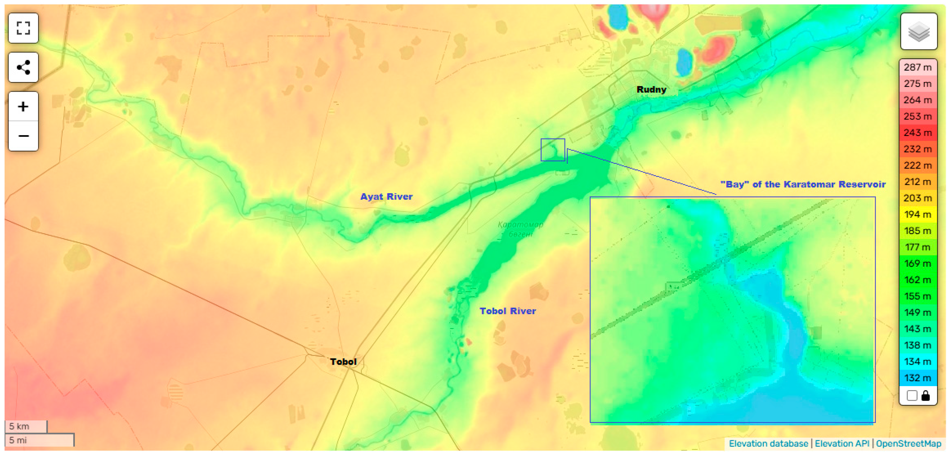
The data on the bay were taken from the entire area of the water body with a boat tack pitch of 50 meters across the current. Only the shallow upper part (about 10% of the area), abundantly overgrown with reeds, remained unexamined.
The studied object (bay) is characterized by a length of about 900 meters, a width of 100-140 meters and a depth interval of up to 6.4 meters. The slope of the bay is about 7.11 o/oo.
Data interpolation for building a digital model and constructing a bathymetric map was performed using 3 different mathematical methods: linear interpolation (mid-segment method), linear regression Z = AX + BY + C and simple kriging.
The isobath map of the bay is shown in Figure 3.
The standard mean square error (MSE) and maximum relative deviation (MRD) are selected as the tools for assessing the quality of interpolation.
MSE allows you to assess the quality of the approximation over the entire interval.
MRD gives peak deviations and allows you to assess the quality of the approximation at the worst point.
The results of comparing methods based on the primary processing of bay data with the summation of data from all runs allow us to state that the regression method for this data set gives the worst result. Kriging with an increase in the step still gives a smaller error, which characterizes it as more preferable.

Table 4.
Estimation of bay depths by different interpolation methods.
| Parameter | Depth (Minimum) | Depth (Maximum) | ||||||
|---|---|---|---|---|---|---|---|---|
| Run step | 10 | 25 | 50 | 100 | 10 | 25 | 50 | 100 |
| Interpolation method | ||||||||
| Linear | 0.800 | 0.400 | 0.130 | 1.540 | 5.540 | 5.250 | 5.490 | 5.360 |
| Planar Regression: Z = AX+BY+C |
0,1353 | 0.009 | 0.016 | 0.001 | 3.054 | 1.073 | 1.096 | 0.707 |
| Kriging | 1.573 | 1.141 | 1.007 | 2.727 | 5.550 | 5.419 | 5.919 | 5.348 |
Table 5.
Estimation of average depth and error of interpolation methods.
| Parameter | Depth (Mean) | MSE (Relative Mean Diff) | ||||||
| Run step | 10 | 25 | 50 | 100 | 10 | 25 | 50 | 100 |
| Interpolation method | ||||||||
| Linear | 4.225 | 4.216 | 4.274 | 4.301 | 0.112 | 0.106 | 0.105 | 0.161 |
| Planar Regression: Z = AX+BY+C |
2.245 | 0.313 | 0.320 | 0.288 | 0.164 | 0.359 | 0.301 | 0.342 |
| Kriging | 4.298 | 4.261 | 4.343 | 4.367 | 0.119 | 0.102 | 0.107 | 0.105 |
To determine the optimal tack pitch of the boat for bathymetric studies, a rectangular polygon was selected in the center of the bay near the Parallel tourist base (Figure 4).
The size of the additional research polygon in the bay is 80x130 meters, where 130 meters is the side across the bay bed. The minimum measured depth according to the bot is 3.55 m, the maximum is 4.98 m.
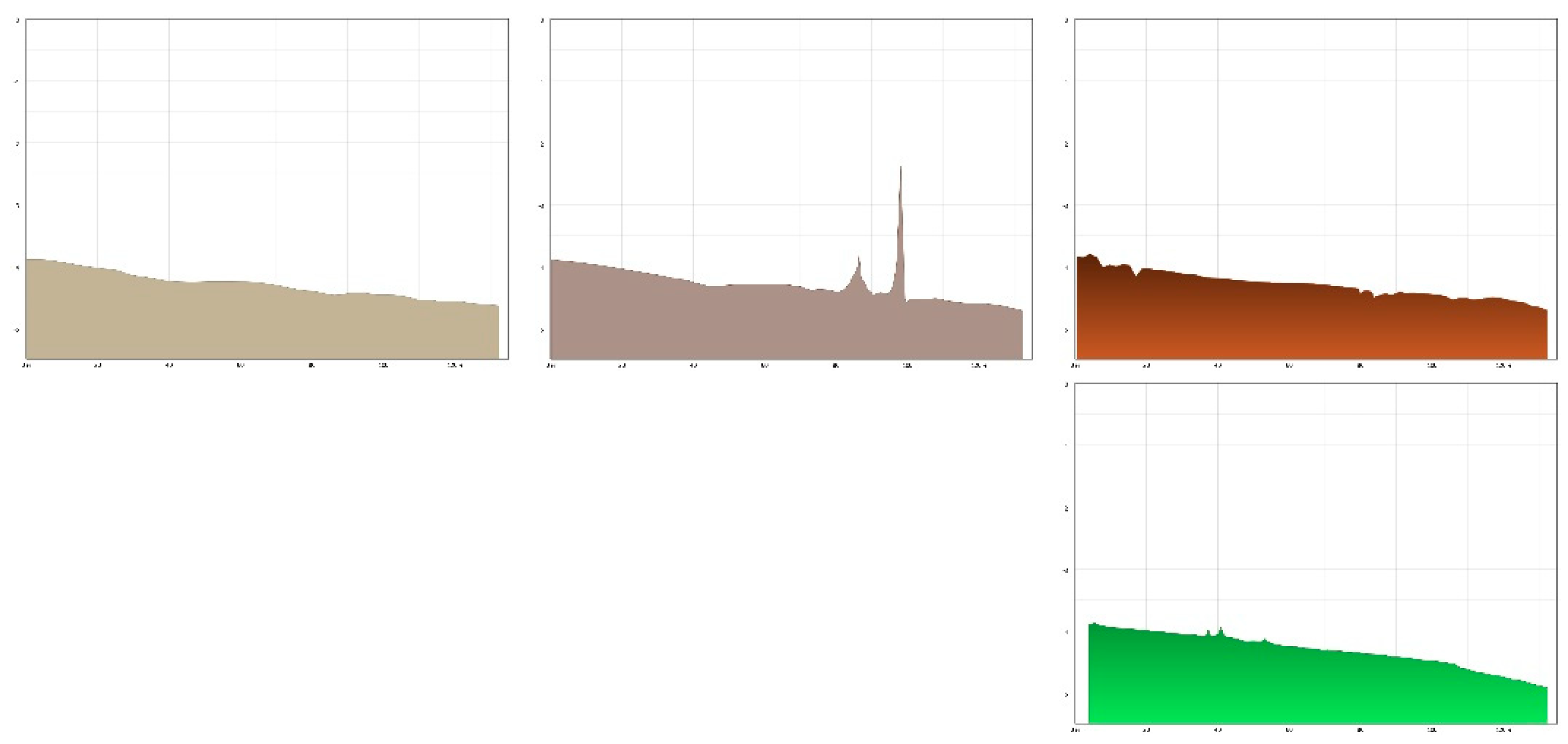
Figure 5.
Bottom relief geometry of section P1 of the bay (along the current, right edge) of the bay polygon for different runs (after 10, 25, 50 and 100 meters). Maximum depth is 4.03 meters.
Figure 5.
Bottom relief geometry of section P1 of the bay (along the current, right edge) of the bay polygon for different runs (after 10, 25, 50 and 100 meters). Maximum depth is 4.03 meters.
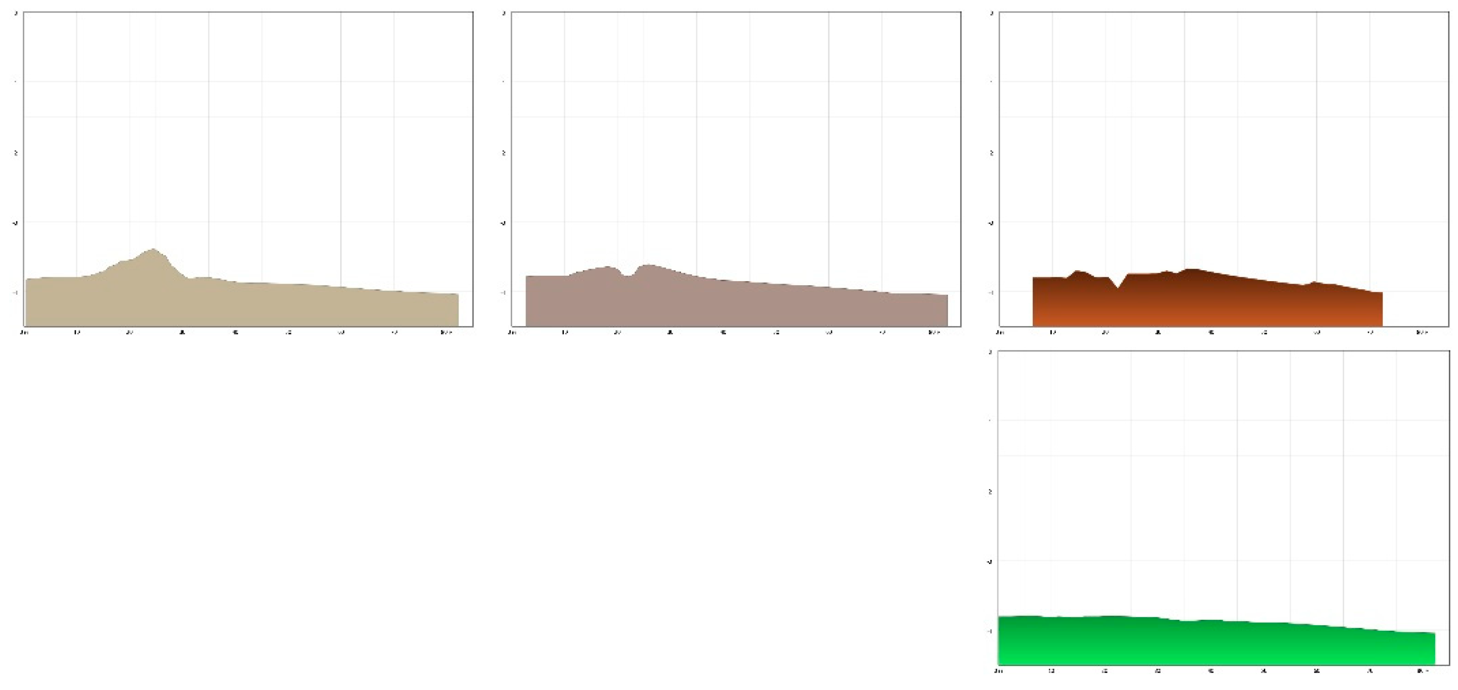
Based on the results of measurements in the polygon of the section locations, the bay bottom slope in the direction of the current is 2.6-5.8 o/oo, across the bay channel – 6.08 o/oo towards the left bank.
Based on the relief shape of the sections, it is clear that with an increase in the tack pitch of the bathymetric boat to 50 meters, local extrema of the bay bottom (an unidentified submerged object) begin to be lost. Although with a fairly flat bottom and the absence of underwater objects, the Pearson correlation coefficient is about 0.9.
Figure 6.
Geometry of the bottom relief of section P2 of the bay (along the current, center) of the bay polygon for different runs (after 10, 25, 50 and 100 meters)
Figure 6.
Geometry of the bottom relief of section P2 of the bay (along the current, center) of the bay polygon for different runs (after 10, 25, 50 and 100 meters)
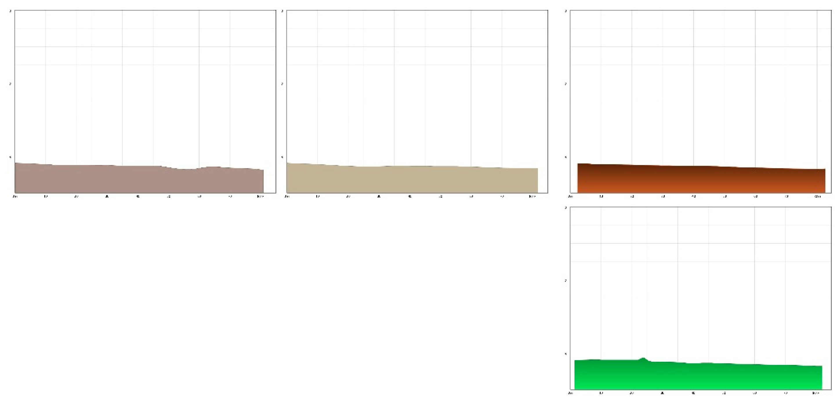
Figure 7.
Geometry of the bottom relief of section P3 of the bay (along the current, left edge) of the bay polygon for different runs (after 10, 25, 50 and 100 meters)
Figure 7.
Geometry of the bottom relief of section P3 of the bay (along the current, left edge) of the bay polygon for different runs (after 10, 25, 50 and 100 meters)
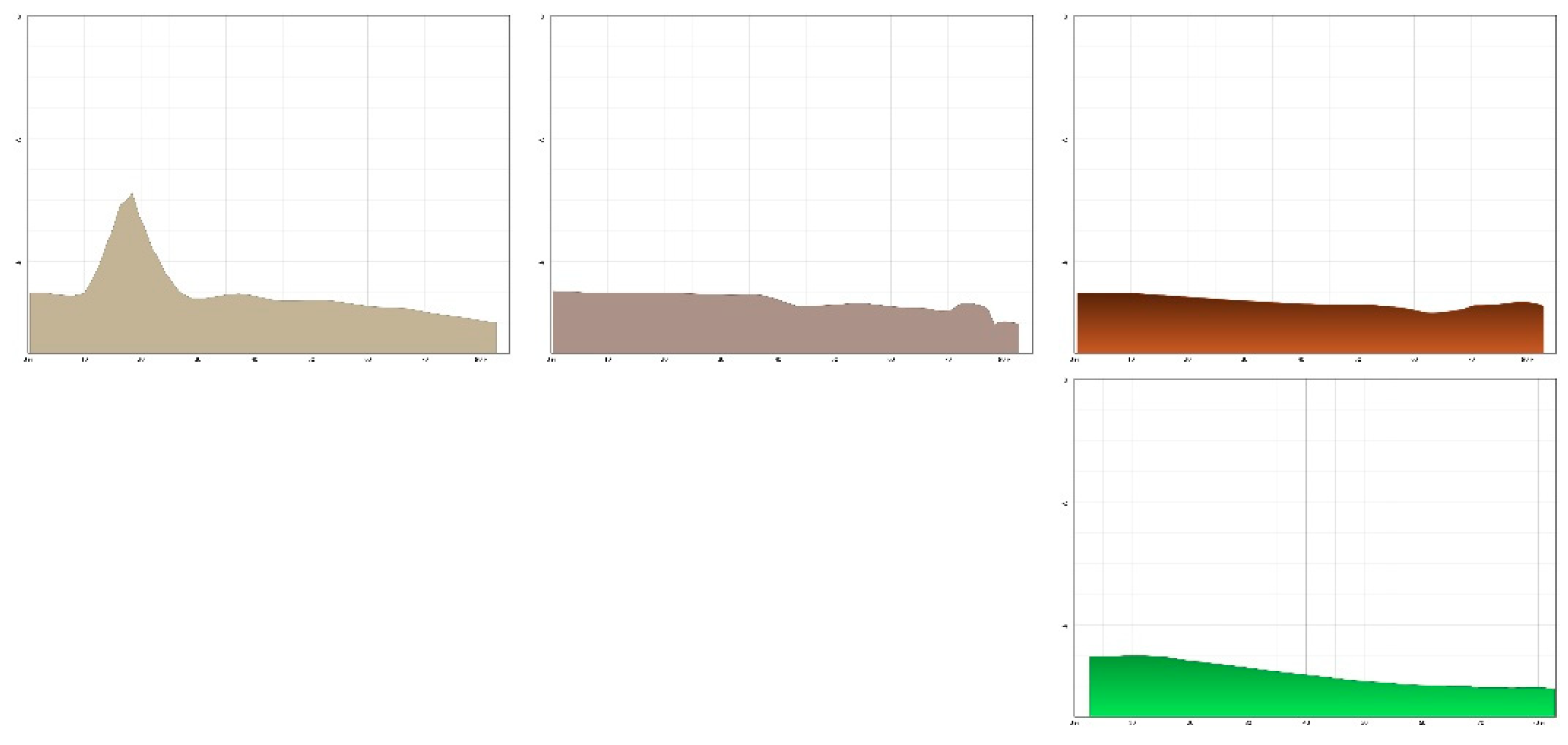
Figure 8.
Geometry of the bottom relief of the section P4 of the bay (across the current) of the bay polygon for different runs (after 10, 25, 50 and 100 meters)
Figure 8.
Geometry of the bottom relief of the section P4 of the bay (across the current) of the bay polygon for different runs (after 10, 25, 50 and 100 meters)
To improve the quality of the initial data, we carried out pre-processing and the pulsation data that did not satisfy the three sigma rule were removed from the input array (the probability of erroneous removal of this pulsation does not exceed 0.28%).
Table 6.
Values of interpolated depths for sections of the bay polygon.
| Section Р1 | Section Р2 | Section Р3 | ||||||||||
| Run step | 10 | 25 | 50 | 100 | 10 | 25 | 50 | 100 | 10 | 25 | 50 | 100 |
| Point | Depth | |||||||||||
| 0 | -3.82 | -3.79 | -3.80 | -3.81 | -4.18 | -4.18 | -4.18 | -4.18 | -4.51 | -4.49 | -4.52 | -4.52 |
| 10 | -3.79 | -3.78 | -3.80 | -3.81 | -4.22 | -4.22 | -4.22 | -4.19 | -4.52 | -4.52 | -4.52 | -4.51 |
| 20 | -3.55 | -3.68 | -3.79 | -3.8 | -4.27 | -4.23 | -4.23 | -4.19 | -3.33 | -4.52 | -4.58 | -4.60 |
| 30 | -3.76 | -3.69 | -3.74 | -3.83 | -4.27 | -4.24 | -4.25 | -4.24 | -4.61 | -4.55 | -4.65 | -4.71 |
| 40 | -3.87 | -3.85 | -3.72 | -3.86 | -4.27 | -4.26 | -4.26 | -4.28 | -4.57 | -4.63 | -4.69 | -4.82 |
| 50 | -3.90 | -3.89 | -3.84 | -3.89 | -4.27 | -4.30 | -4.28 | -4.29 | -4.64 | -4.71 | -4.71 | -4.92 |
| 60 | -3.94 | -3.94 | -3.87 | -3.93 | -4.29 | -4.32 | -4.31 | -4.31 | -4.73 | -4.74 | -4.80 | -4.99 |
| 70 | -4.00 | -4.01 | -4.00 | -4.00 | -4.32 | -4.32 | -4.33 | -4.33 | -4.83 | -4.81 | -4.74 | -5.03 |
| 80 | -4.03 | -4.04 | -4.02 | -4.04 | -4.33 | -4.36 | -4.34 | -4.36 | -4.98 | -4.99 | -4.67 | -5.03 |
The data for cross-section P4 were obtained in a similar manner.
In order to prove that the curves representing the bottom relief geometry for different runs are similar, in addition to the correlation coefficient, it was decided to use the curve similarity coefficient. For this purpose, the probability that one relief cross-section can be transformed into another by scaling along the depth axis was checked, i.e., to check that the sections are geometrically similar.
For this purpose, a modified formula was used to prove the similarity of curves:
where y1 and y2 – are the depths of the reference and compared sections;
k –is the curve similarity coefficient.
All linear dimensions of one curve should be proportional to similar dimensions of another curve with the same similarity coefficient. Then, mathematically, this can be expressed through the correspondence of the coordinate points of the two curves:
For a set of cross-section points of two reliefs, the authors selected the worst similarity coefficient, which characterizes the worst similarity of the possible options in the comparison area. And the run with a step of 10 meters is again used as a reference.
Table 7.
Pearson correlation coefficient and similarity coefficient of relief curves, MSE and MRD measurements from the step of runs.
Table 7.
Pearson correlation coefficient and similarity coefficient of relief curves, MSE and MRD measurements from the step of runs.
| Parameter | Р1 | Р2 | Р3 | Р4 | ||||||||
|---|---|---|---|---|---|---|---|---|---|---|---|---|
| Run step | 25 | 50 | 100 | 25 | 50 | 100 | 25 | 50 | 100 | 25 | 50 | 100 |
| MSE | 0.00 | 0.01 | 0.01 | 0.00 | 0.00 | 0.00 | 0.16 | 0.19 | 0.21 | 0.00 | 0.00 | 0.01 |
| MRD | 0.02 | 0.04 | 0.00 | 0.01 | 0.01 | 0.02 | 0.01 | 0.06 | 0.00 | 0.00 | 0.01 | 0.04 |
| Pearson correlation coefficient | 0.93 | 0.69 | 0.85 | 0.90 | 0.94 | 0.87 | 0.60 | 0.44 | 0.57 | 1.00 | 0.99 | 0.96 |
| Similarity coefficient | 0.99 | 0.97 | 0.96 | 0.99 | 0.98 | 0.99 | 0.99 | 0.94 | 0.92 | 0.98 | 0.97 | 0.95 |
Thus, based on the calculations performed (Fig. 9), it can be stated that in order to ensure the stated accuracy of at least 10%, it is necessary to conduct a field study of the reservoir area with a boat tack pitch of no more than 200 meters.
3.4. Evaluation of the Compliance of the Tobol River Bed with the Conditions Taken as the Standard "Bay"
To check the correspondence of the reservoir to the bay, a comparative analysis of the obtained average bay cross-sections with the obtained average reservoir cross-sections was carried out. The correlation coefficient and curve similarity index were used for the assessment.
Figure 10.
Layout of sections along the Ayat (P1) and Tobol (P2) rivers, as well as sections P3 and P4 at the confluence of these rivers.
Figure 10.
Layout of sections along the Ayat (P1) and Tobol (P2) rivers, as well as sections P3 and P4 at the confluence of these rivers.
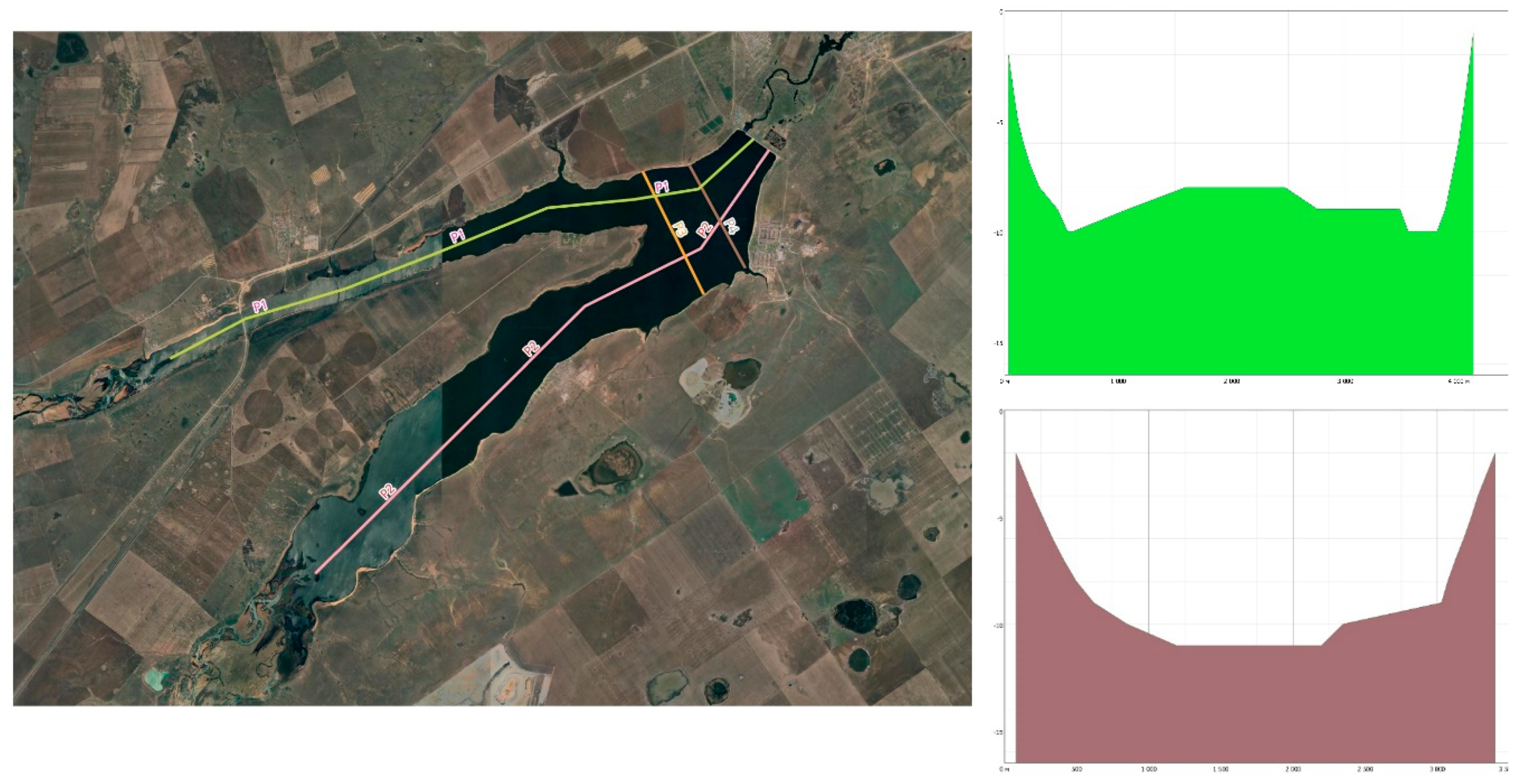
The constructed profile P1 along the Ayat river bed allows us to speak of a bottom slope of 0.5 °/°°. The bottom slope of the bay exceeds the slope of the Ayat river within the reservoir by 5 times. The relief is rich in whirlpools. The characteristic repeating peaks of depth minima are most likely caused not by shallows, but by an error in the interpolation method due to insufficient initial data (gaps between polygons, which explains their periodicity, coinciding with the zones of absence of boat tacks) and require additional field bathymetric surveys (planned for the warm period of summer 2025).
Figure 11.
Section P1 along the Ayat River in QGIS and linear interpolant in MS Excel of the Ayat River bed in the reservoir area
Figure 11.
Section P1 along the Ayat River in QGIS and linear interpolant in MS Excel of the Ayat River bed in the reservoir area
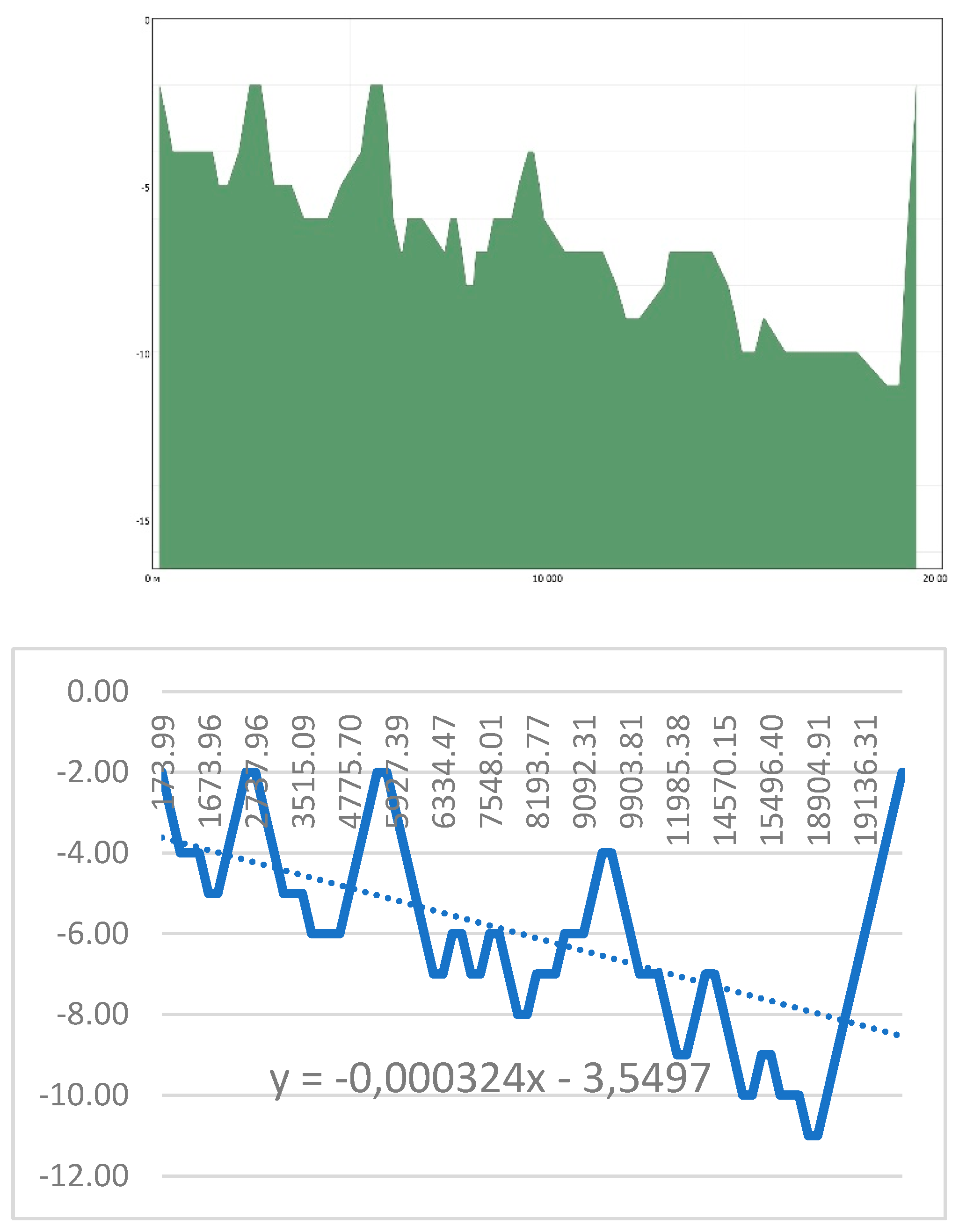
Table 8.
Interpolation data and Pearson correlation coefficients for sections P1 (Ayat), P2 (Tobol) and three sections (P1b Z2b Z3) of the reservoir “bay”.
Table 8.
Interpolation data and Pearson correlation coefficients for sections P1 (Ayat), P2 (Tobol) and three sections (P1b Z2b Z3) of the reservoir “bay”.
| Depth, m | Pirson Аyat | Pirson Tobol | ||||||||||
|---|---|---|---|---|---|---|---|---|---|---|---|---|
| Distance, m | 0 | 10 | 20 | 30 | 40 | 50 | 60 | 70 | 80 | |||
| r. Ayat | P1 | -3.55 | -3.55 | -3.56 | -3.56 | -3.56 | -3.57 | -3.57 | -3.57 | -3.58 | ||
| r. Tobol | P2 | -5.44 | -5.45 | -5.45 | -5.46 | -5.46 | -5.47 | -5.47 | -5.48 | -5.48 | ||
| “Bay” | P1 | -3.82 | -3.79 | -3.55 | -3.76 | -3.87 | -3.90 | -3.94 | -4.03 | -4.00 | 0.74 | 0.74 |
| P2 | -4.18 | -4.22 | -4.27 | -4.27 | -4.27 | -4.27 | -4.29 | -4.32 | -4.33 | 0.93 | 0.93 | |
| P3 | -4.51 | -4.52 | -3.33 | -4.61 | -4.57 | -4.64 | -4.73 | -4.83 | -4.98 | 0.54 | 0.54 | |
According to the table data, we see a high correlation between the values of the bottom relief (depths) in the middle of the Ayat River (within the boundaries of the reservoir) and the depths in the middle (flowing part of the bay), which allows us to talk about the applicability of the proposed method for assessing the accuracy of the tack pitch for the Ayat River.
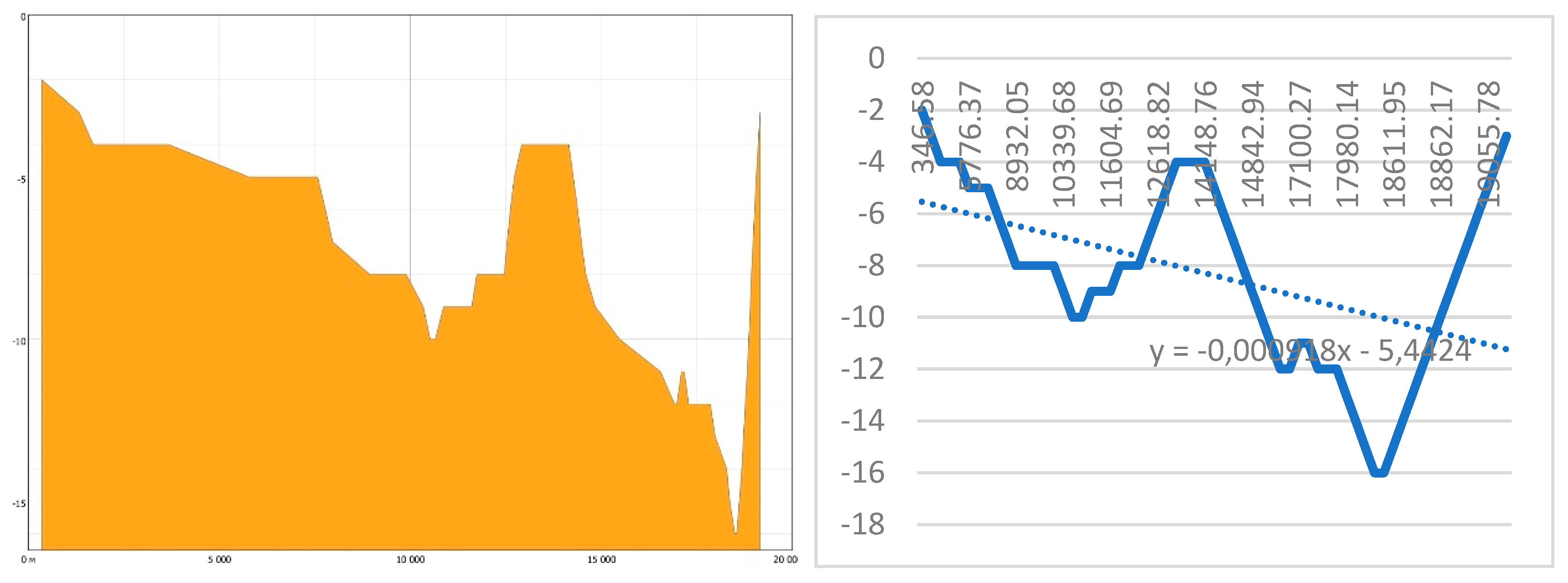
The constructed profile along the Tobol River bed allows us to state that the current bottom slope is 0.8 o/oo. The bottom slope of the bay exceeds the slope of the Tobol River within the reservoir by 3 times. The relief is quite smooth. The existing peak may also correspond to a break in the drone's measurement runs (additional field bathymetric surveys are required, planned for the warm period of 2025).
The correlation of the Tobol River data with the depths of the bay is identical to the Ayat data.
Figure 12.
Section P2 along the Tobol River in QGIS and linear interpolant in MS Excel of the Tobol River bed in the reservoir area.
Figure 12.
Section P2 along the Tobol River in QGIS and linear interpolant in MS Excel of the Tobol River bed in the reservoir area.
Based on the results of the studies, it can be stated that for river beds with smoothed bottom reliefs corresponding to the flow of the Ayat and Tobol Rivers within the boundaries of the Karatomar Reservoir, the dependence of the measurement error on the tack pitch is of the following nature:
where L is the tack pitch across the river flow.
3.5. Modeling the State of the Kartomar Reservoir
The constructed map of the Karatomar reservoir in QGis based on the bathymetric measurements carried out with a step of 200 meters is presented in Figure 13.
Based on the constructed map, reservoir depth polygons were modeled with a depth step of 1 meter (if necessary, a map with any depth step can be constructed). The reservoir surface area and current (corresponding to 98% full as of 14/07/2024) reservoir volumes within the boundaries selected from the space image were also calculated.
Table 9.
Results of interpolation of depth polygons of current values of the Karatomar reservoir.
| Depth, m | Mirror area by depth | Bowl volume by depth | ||
|---|---|---|---|---|
| km2 | % of maximum | km3 | % of maximum | |
| 0 | 61.466 | 100.00 | 367.049 | 100.00 |
| 1 | 55.254 | 89.89 | 305.582 | 83.25 |
| 2 | 50.716 | 82.51 | 250.329 | 68.20 |
| 3 | 45.473 | 73.98 | 199.613 | 54.38 |
| 4 | 38.947 | 63.36 | 154.140 | 41.99 |
| 5 | 31.860 | 51.83 | 115.192 | 31.38 |
| 6 | 24.899 | 40.51 | 83.332 | 22.70 |
| 7 | 20.794 | 33.83 | 58.433 | 15.92 |
| 8 | 16.750 | 27.25 | 37.638 | 10.25 |
| 9 | 11.618 | 18.90 | 20.889 | 5.69 |
| 10 | 5.739 | 9.34 | 9.271 | 2.53 |
| 11 | 2.137 | 3.48 | 3.531 | 0.96 |
| 12 | 0.878 | 1.43 | 1.394 | 0.38 |
| 13 | 0.309 | 0.50 | 0.516 | 0.14 |
| 14 | 0.129 | 0,21 | 0.208 | 0.06 |
| 15 | 0.061 | 0.10 | 0.079 | 0.02 |
| 16 | 0.018 | 0.03 | 0.018 | 0.00 |
A comparative analysis of the planned indicators of the reservoir (for the period of 1966) and those obtained as a result of the bathymetric study is summarized in Table 10.
In our opinion, significant changes in the reservoir parameters are related to silting of the reservoir bowl (over the past 25 years, there has been a significant decrease in the discharge of flood waters, which did not contribute to the natural washing of the Tobol and Ayat river beds in the reservoir bowl from alluvial rocks, and dredgers did not carry out work to clean and deepen the bottom) and overgrowing of the banks with vegetation (the reservoir surface area in the upper part of the Tobol River has been significantly reduced). A study of the bottom sediments of the Karatomar Reservoir is planned for the period spring-summer 2025.
4. Discussion
As a result of the study conducted by the authors of the article, the following answers to the research questions were obtained.
First, a comparative analysis of interpolation methods on the data of the "bay" of the Karatomar reservoir allows us to state the preference for using the simple cry method over regression methods with an increase in the tack step.
The correlation of the geomorphology parameters of the "bay" with the geomorphology of the Tobol and Ayat rivers in the reservoir zone allows us to state the possibility of transferring the obtained dependencies to the water areas of these rivers.
Achieving the required accuracy of bathymetric studies, with an error of less than 10%, with the current geomorphology of the bottom of the Karatomar reservoir (as a plain-type reservoir with a bottom slope of about 0.5-7.11 o/oo) is possible if the step of the drone tacks does not exceed 200 meters. However, even if this condition was met, during the study of the water area, areas with significant deviations in relief were obtained, the clarification of which requires additional field studies.
Secondly, over 78 years of operation, the actual parameters of the Karatomar reservoir have undergone significant changes (the total volume of the reservoir has decreased by more than 50%, the area of the water surface has decreased by more than 30%, the maximum depth has decreased by more than 18%). A similar picture of a significant deterioration in the characteristics of a hydraulic structure is characteristic not only of the Karatomar reservoir, but also of the Verkhnetobol reservoir, studied by the authors of the article (it is possible to assume that other hydraulic structures in the region are in a similar situation).
These changes are caused by significant overgrowing of shallow sections of the Tobol River with reeds in the upper zone of the reservoir and silting of the reservoir bowl.
Such unaccounted changes in the condition of hydraulic structures could lead to additional management difficulties and risks during the flood of 2024, and a significant decrease in water reserves could further affect the prospects for sustainable development of the region.
Due to the significant impact of the Karatomar reservoir as one of the main reservoirs of the Kostanay region on the economy of Kazakhstan, we believe that additional research is needed to study the nature of siltation and develop measures to restore the parameters of the hydraulic structure under study.
Author Contributions
Conceptualization, Mikhail Zarubin and Vadim Chashkov; methodology, Mikhail Zarubin and Vadim Chashkov; software, Olga Salykova; validation, Aliya Yskak; formal analysis, Mikhail Zarubin; investigation, Mikhail Zarubin and Olga Salykova; resources, Vadim Chashkov and Seitbek Kuanyshbayev; data curation, Artem Bashev and Adil Nurpeisov; writing—original draft preparation, Mikhail Zarubin; writing—review and editing, Mikhail Zarubin; visualization, Mikhail Zarubin; supervision, Almabek Nugmanov; project administration, Almabek Nugmanov; funding acquisition, Seitbek Kuanyshbayev. All authors have read and agreed to the published version of the manuscript.
Funding
This research was funded by Ministry of Science and Higher Education of the Republic of Kazakhstan, grant number BR21881993 “Organization of a system of operational monitoring of water resources and environmental control of hydrotechnic engineering structures in Northern Kazakhstan” and “The APC was funded by number BR21881993 “Organization of a system of operational monitoring of water resources and environmental control of hydrotechnic engineering structures in Northern Kazakhstan”.
Data Availability Statement
Bathymetric research data are available on the website of the Akhmet Baitursynov Kostanay Regional University.
Conflicts of Interest
The authors declare no conflicts of interest.
Abbreviations
The following abbreviations are used in this manuscript:
| LI | Interpolation method. Linear interpolation (midpoint method) |
| GPI | Interpolation method. Interpolation by the global polynomial method |
| LPI | Interpolation method. Interpolation by the local polynomial method |
| IDW | Interpolation method. Interpolation by the inverse distance weighted method |
| RBF | Interpolation method. Interpolation based on the application of radial basis functions |
| Kriging | Interpolation method. Ordinary, simple, universal, indicator, probabilistic, disjunctive and empirical Bayesian kriging. |
| RMSE | Root mean square error |
| SRTM | Shuttle Radar Topography Mission |
| MLP | Multilayer perceptron |
| RBFN | Radial basis function neural network |
| FNN | Back propagation neural network |
| DNN | Deep neural network |
| CapsNet | Capsule neural networks |
| MSE | Mean square error |
| MRD | Maximum relative deviation |
References
- Cooley, S. W., Ryan, J. C., Smith, L. C. Human alteration of global surface water storage variability. Nature, 2021, 591(7848), pp. 78–81. [CrossRef]
- Chao, B., Wu, Y., Li, Y. Impact of artificial reservoir water impoundment on global sea level. Science, 2008, 320(5873), pp. 212–214. [CrossRef]
- Williamson, C. E., Saros, J. E., Vincent, W. F., Smol, J. P. Lakes and reservoirs as sentinels, integrators, and regulators of climate change. Limnology & Oceanography, 2009, 54 (6 part 2), pp. 2273–2282. [CrossRef]
- On approval of the Concept for the development of the water resources management system of the Republic of Kazakhstan for 2024–2030, Resolution of the Government of the Republic of Kazakhstan dated February 5, 2024. No. 66. Available online: https://adilet.zan.kz/rus/docs/P2400000066 (accessed on 27 March 2025).
- Yigzaw, W., Li, H. Y., Demissie, Y., Hejazi, M. I., Leung, L. R., Voisin, N., Payn, R. A new global storage-area-depth data set for modeling reservoirs in land surface and earth system models. Water Resources Research, 2018, 54(12), pp. 386. [CrossRef]
- Li, Y., Gao, H., Jasinski, M. F., Zhang, S., Stoll, J. D. Deriving high-resolution reservoir bathymetry from ICESat-2 prototype photon-counting lidar and landsat imagery. IEEE Transactions on Geoscience and Remote Sensing, 2019, 57(10), pp. 7883–7893. [CrossRef]
- Rodriguez, E., Morris, C., Belz, J., Chapin, E., Martin, J., Daffer, W., Hensley, S. An assessment of the SRTM topographic products, Technical Report JPL D-31639, Jet Propulsion Laboratory, Pasadena, California, 2005, 143 p.
- Zhang, K., Gann, D., Ross, M., Robertson, Q., Sarmiento, J., Santana, S., Rhome, J., Fritz, C. Accuracy assessment of ASTER, SRTM, ALOS, and TDX DEMs for Hispaniola and implications for mapping vulnerability to coastal flooding. Remote Sensing of Environment, 2019, 225, pp. 290–306. [CrossRef]
- Hao, Z., Chen, F., Jia, X., Cai, X., Yang, C., Du, Y., Ling, F. GRDL: A new global reservoirarea-storage-depth data set derivedthrough deep learning-based bathymetryreconstruction. Water ResourcesResearch,, 2024, 60. [CrossRef]
- Bandini, F., Olesen, D., Jakobsen, J., Kittel, C., Wang, S., Garcia, M., Bauer-Gottwein, P. Bathymetry observations of inland water bodies using a tethered single-beam sonar controlled by an unmanned aerial vehicle. Hydrology and Earth System Sciences, 2018, 22(8), pp. 4165–4181. [CrossRef]
- Pirani, F., Modarres, R. Geostatistical and deterministic methods for rainfall interpolation in the Zayandeh. Hydrological sciences journal, 2020, 65(16), pp. 2678–2692. [CrossRef]
- Zarubin, M., Zarubina, V., Jamanbalin, K., Akhmetov, D., Yessenkulova, Z., Salimbayeva, R. Digital Technologies as a Factor in Reducing the Impact of Quarries on the Environment. Environmental and Climate Technologies, 2021, 25, pp. 436–454. [CrossRef]
- Dovile, K., Zenonas, N., Raimondas, Č., Minvydas, R. An extended Prony’s interpolation scheme on an equispaced grid. Open Mathematics, 2015, 13(1), pp. 000010151520150031. [CrossRef]
- Skorokhodov, I. Interpolating Points on a Non-Uniform Grid using a Mixture of Gaussians, 2020, Available online: https://arxiv.org/pdf/2012.13257 (accessed on 27 March 2025).
- Gilewski, P. Impact of the Grid Resolution and Deterministic Interpolation of Precipitation on Rainfall-Runoff Modeling in a Sparsely Gauged Mountainous Catchment. Water, 2021, 13(2):230, doi:doi: 10.3390/W13020230.
- Ben-Or, M., Tiwari, P. A deterministic algorithm for sparse multivariate polynomial interpolation. In Proceedings of the twentieth annual ACM symposium on Theory of computing (STOC '88). Association for Computing Machinery, 1988, pp. 301–309. [CrossRef]
- Biernacik, P., Kazimierski, W., Wlodarczyk-Sielicka, M. Comparative Analysis of Selected Geostatistical Methods for Bottom Surface Modeling. Sensors, 2023, 23, 3941. [CrossRef]
- Alcaras, E., Amoroso, P.P. , Parente, C. The Influence of Interpolated Point Location and Density on 3D Bathymetric Models Generated by Kriging Methods: An Application on the Giglio Island Seabed (Italy). Geosciences (Switzerland), 2022, 12. 62. [CrossRef]
- Kazimierski, W., Wlodarczyk-Sielicka, M. Comparative Analysis of Selected Geostatistical Methods for Bottom Surface Modeling. Sensors, 2023, 23(8), pp. 3941-3941, doi:doi: 10.3390/s23083941.
- Chowdhury, M., Alouani, A.T., Hossain, F. Comparison of Ordinary Kriging and Artificial Neural Network for Spatial Mapping of Arsenic Contamination of Groundwater. Stochastic Environmental Research & Risk Assessment, 2008, 24, pp. 1-7. [CrossRef]
- Janowicz, K., Gao, S., McKenzie, G., Hu, Y., Bhaduri, B. GeoAI: spatially explicit artificial intelligence techniques for geographic knowledge discovery and beyond. International Journal of Geographical Information Science, 2019, 34 (4), pp. 625-636. [CrossRef]
- Zarubin, M., Zarubina, V. Results of using neural networks for technological processes control of iron mill. Journal Energy procedia, 2016, 95, pp. 512-516, doi:DOI:10.1016/j.egypro.2016.09.077.
- Yu-Len, H., Ruey-Feng, C. MLP interpolation for digital image processing using wavelet transform. In Proceedings of the Acoustics, Speech, and Signal Processing, 06 (ICASSP '99). IEEE Computer Society, USA, 1999, pp. 3217–3220. doi:0.1109/ICASSP.1999.757526.
- Nevtipilova, V., Pastwa, J., Boori, M. S., Vozenilek, V. Testing multilayer perceptron (MLP) for spatial interpolation. Interexpo Geo-Siberia, 2014, pp. 33-51. Available online: https://cyberleninka.ru/article/n/testing-multilayer-perceptron-mlp-for-spatial-interpolation (accessed on 27 March 2025).
- Yeh, I., Huang, K.-C., Kuo, Y.-H.. Spatial interpolation using MLP–RBFN hybrid networks. International Journal of Geographical Information Science, 2013, 27, pp. 1884-1901. [CrossRef]
- Gotway, C., Ferguson, R., Hergert, G., Peterson, T. Comparison of Kriging and Inverse-Distance Methods for Mapping Soil Parameters. Soil Science Society of America Journal - SSSAJ, 1996, pp. 60. [CrossRef]
- Qian, Y. , Ghorbanidehno, H., Lee, J.H. , Farthing, M., Hesser, T. , Kitanidis, P.K., Darve, E.F. Applications of Deep Neural Network to Near-shore Bathymetry with Sparse Measurements. American Geophysical Union, Fall Meeting 2019, abstract #EP43C-04., 2019. Available online: https://ui.adsabs.harvard.edu/abs/2019AGUFMEP43C..04Q/abstract (accessed on 27 March 2025).
- Mazzia, V., Salvetti, F., Chiaberge, M. Efficient-CapsNet: capsule network with self-attention routing. Scientific Reports, 2021, 11(1):14634. [CrossRef]
- Nurpeisova, M.B., Zharkimbaev, B.M. Geodesy, 2002.
- Neumann, J. Maximum depth and average depth of lakes. Journal of the Fisheries Board of Canada, 1959, 16(6), pp. 923–927. [CrossRef]
- Anderson, D. A note on the morphology of the basins of the Great Lakes. Journal of the Fisheries Board of Canada, 1961, 18(2), pp. 273–277. [CrossRef]
- Lehman, J. T. Reconstructing the rate of accumulation of lake sediment: The effect of sediment focusing. Quaternary Research, 1975, 5(4), pp.541–550.
- Carpenter, S. R. Lake geometry: Implications for production and sediment accretion rates. Journal of Theoretical Biology, 1983, 105(2), pp.273–286. [CrossRef]
- Gao, H., Birkett, C., Lettenmaier, D. Global monitoring of large reservoir storage from satellite remote sensing. Water Resources Research, 2012, 48(9), W09504. [CrossRef]
- Wang, Z., Xie, F., Ling, F., Du, Y. Monitoring surface water inundation of Poyang Lake and Dongting Lake in China using Sentinel-1 SAR images. Remote Sensing, 2022, 14(14), 3473. [CrossRef]
- Zhen Hao, Fang Chen, Xiaofeng Jia, Xiaobin Cai, Chao Yang, Yun Du, Feng Ling. GRDL: A New Global Reservoir Area-Storage-Depth Data Set Derived Through Deep Learning-Based Bathymetry Reconstruction. Water Resources Research, 2024, 1(60). [CrossRef]
- Yao, F., Minear, J.T., Rajagopalan, B., Wang, C., Yang, K., Livneh, B. Estimating reservoir sedimentation rates and storage capacity losses using high-resolution Sentinel-2 satellite and water level data. Geophysical Research Letters, 2023, 50(16). [CrossRef]
- Liu, K., Song, C., Wang, J., Ke, L., Zhu, Y., Jingying, Z., Luo, Z.L., Remote sensing-based modeling of the bathymetry and water storage for channel-type reservoirs worldwide. Water Resources Research, 2020, 56(11). [CrossRef]
- Yun, H.-S., Cho, J.-M. Hydroacoustic Application of Bathymetry and Geological Survey for Efficient Reservoir Management. Journal of the Korean Society of Surveying, Geodesy, Photogrammetry and Cartography, 2011, 29. [CrossRef]
- Madden, J. D. Coastline delineation by aerial photography. Australian Surveyor, 1978, 29(2), pp.76–82. [CrossRef]
- Gonçalves, J., Bastos, M., Pinho, J., Granja, H. (Digital aerial photography to monitor changes in coastal areas based on direct georeferencing, 5th EARSeL Workshop on Remote Sensing of the Coastal ZoneAt, Prague, Czech Republic, 2011, Available online: https://www.researchgate.net/publication/360427485_DIGITAL_AERIAL_PHOTOGRAPHY_TO_MONITOR_CHANGES_IN_COASTAL_AREAS_BASED_ON_DIRECT_GEOREFERENCING (accessed on 27 March 2025).
- Tyszkowski, S., Zbucki, Ł., Kaczmarek, H., Duszyński, F., Strzelecki, M. Detection of Coastal Changes along Rauk Coasts of Gotland, Baltic Sea. Remote Sens, 2023, 15, 1667. [CrossRef]
- Lubczonek, J., Kazimierski, W., Zaniewicz, G., Lacka, M. Methodology for Combining Data Acquired by Unmanned Surface and Aerial Vehicles to Create Digital Bathymetric Models in Shallow and Ultra-Shallow Waters. Remote Sens, 2022, 14, 105. [CrossRef]
- Lubczonek, J., Wlodarczyk-Sielicka, M., Lacka, M., Zaniewicz, G. Methodology for Developing a Combined Bathymetric and Topographic Surface Model Using Interpolation and Geodata Reduction Techniques. Remote Sens, 2021, 13, 4427. [CrossRef]
- Han, D. Comparison of Commonly Used Image Interpolation Methods. In Proceedings of the ICCSEE 2013, Hangzhou, China.
- Jiao, Y., Zhang, F., Huang, Q., Liu, X., Li, L. Analysis of Interpolation Methods in the Validation of Backscattering Coefficient Products. Sensors, (2023, 23, 469. https://doi.org/10.3390/s23010469.
- Weather in Rudny in July 2024. Available online: https://belkraj.by/pogoda/kazakhstan/l1519843/rudnyy/july (accessed on 01 September 2024).
- Tobol. Ministry of Natural Resources of Russia. State Water Register, 2009.
Figure 1.
Fragments of Sentinel-2_L2A images from 06/14/2024 and 07/04/2024 when constructing the shoreline of the Karatomar reservoir, a classified image of the reservoir in NDWI format with contouring and a contouring zone of the water surface on a topographic plan.
Figure 1.
Fragments of Sentinel-2_L2A images from 06/14/2024 and 07/04/2024 when constructing the shoreline of the Karatomar reservoir, a classified image of the reservoir in NDWI format with contouring and a contouring zone of the water surface on a topographic plan.
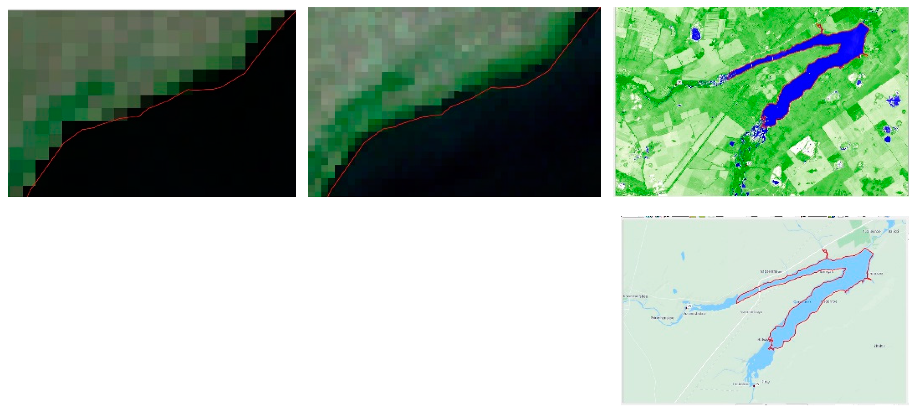
Figure 2.
Scheme of hydraulic structures of Kostanay region on the Tobol river
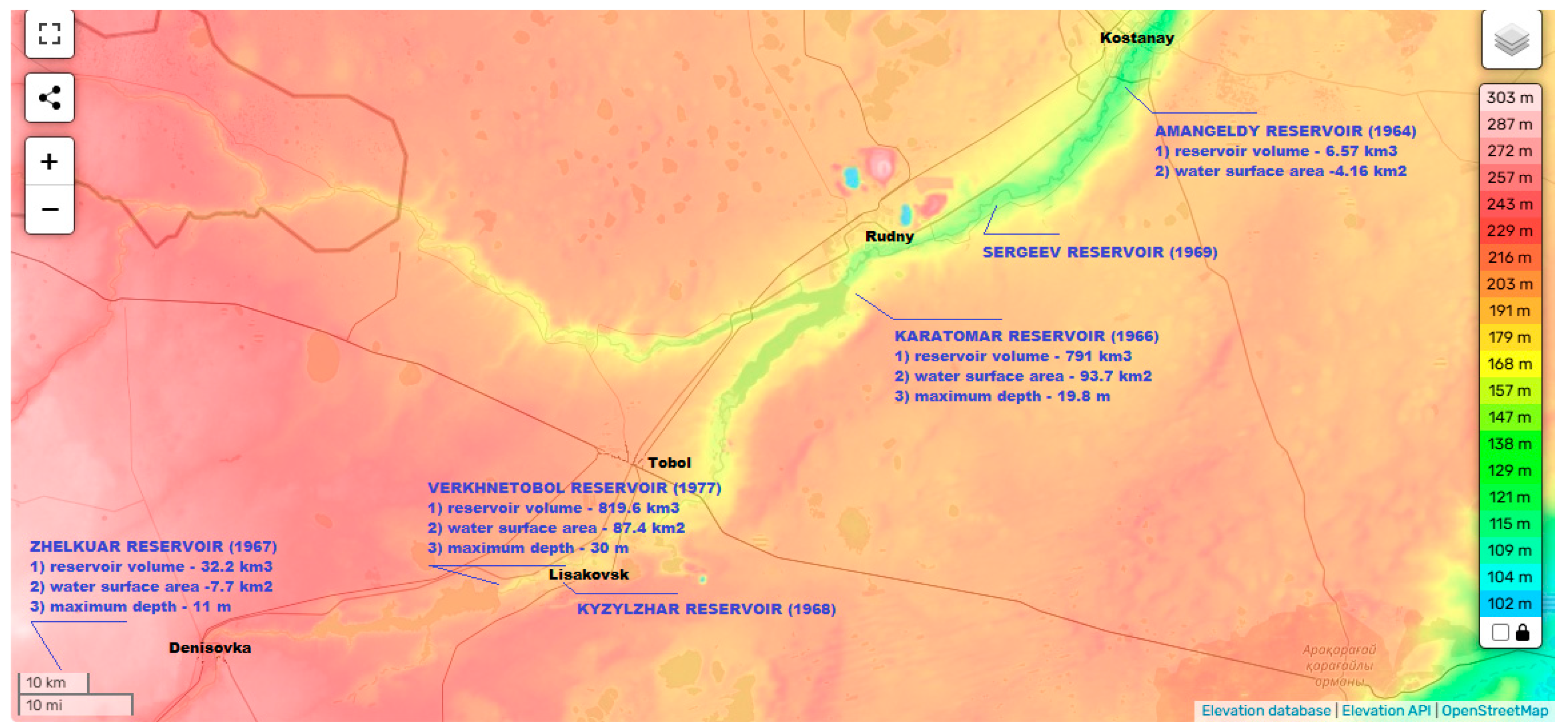
Figure 3.
Digital model of the bay polygon (isobath map)
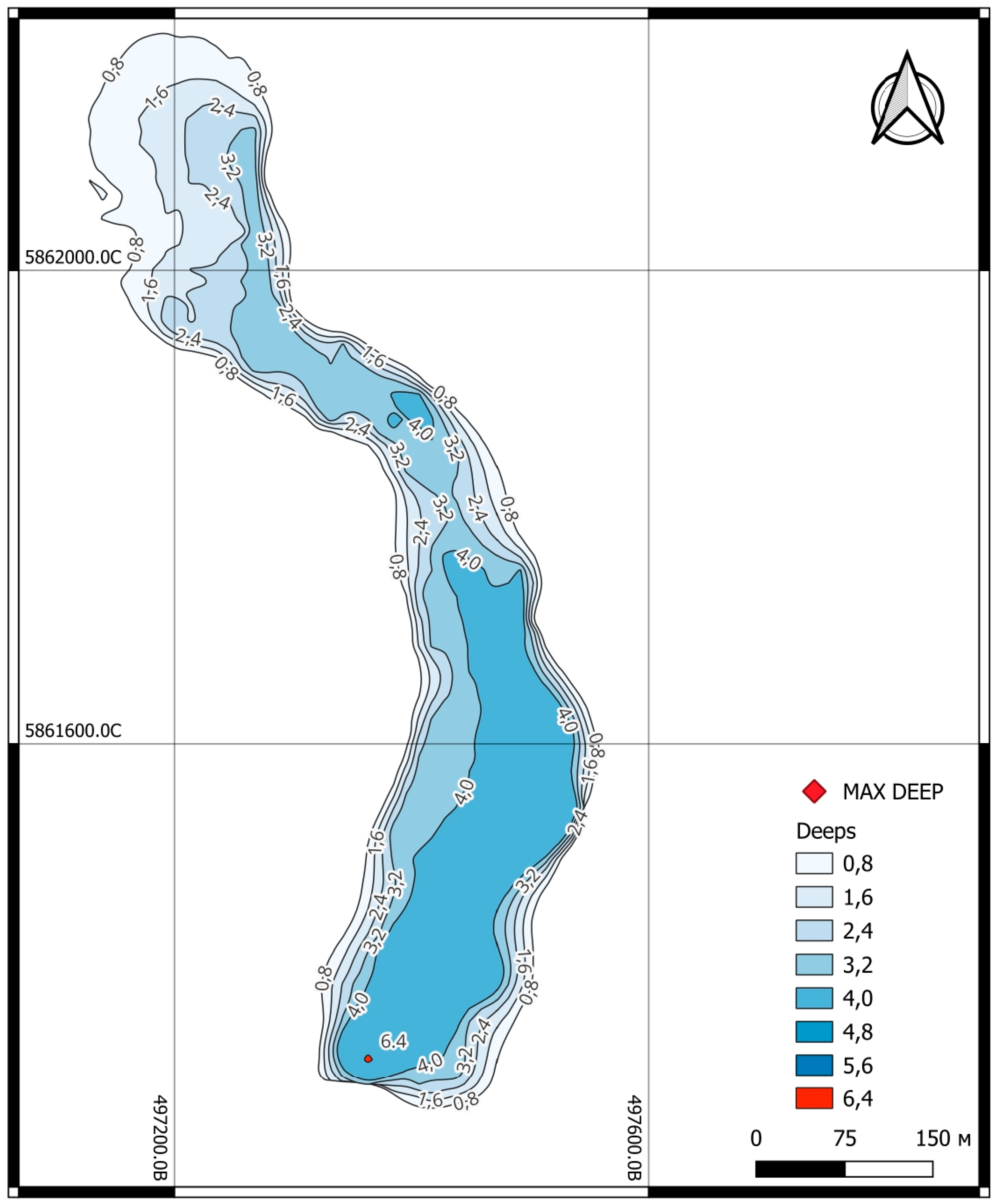
Figure 4.
Map of the additional research polygon and the location of the polygon sections
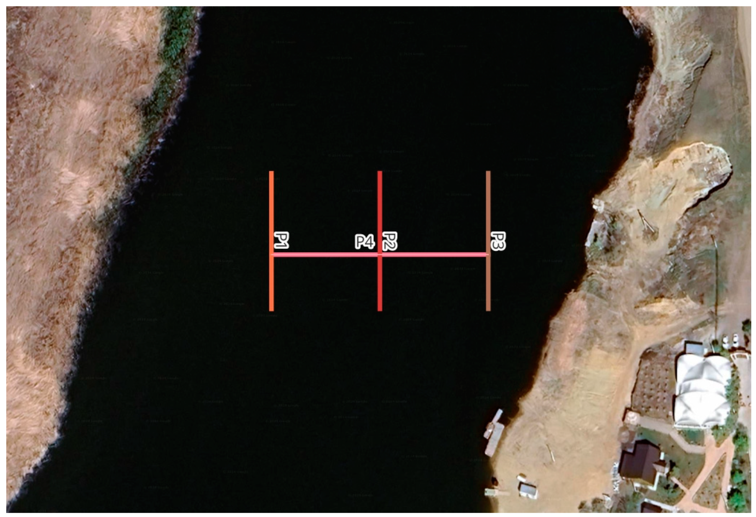
Figure 9.
Forecast of changes in MSE and MRD for the bay from the boat tack pitch
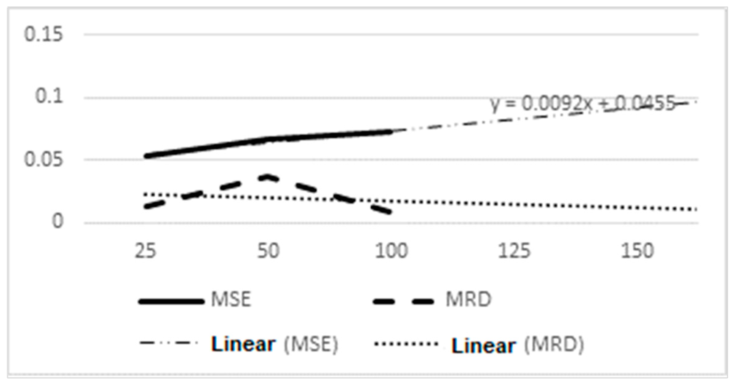
Figure 13.
Map of the Ayat and Tobol isobaths within the boundaries of the Karatomarskoye reservoir.
Figure 13.
Map of the Ayat and Tobol isobaths within the boundaries of the Karatomarskoye reservoir.
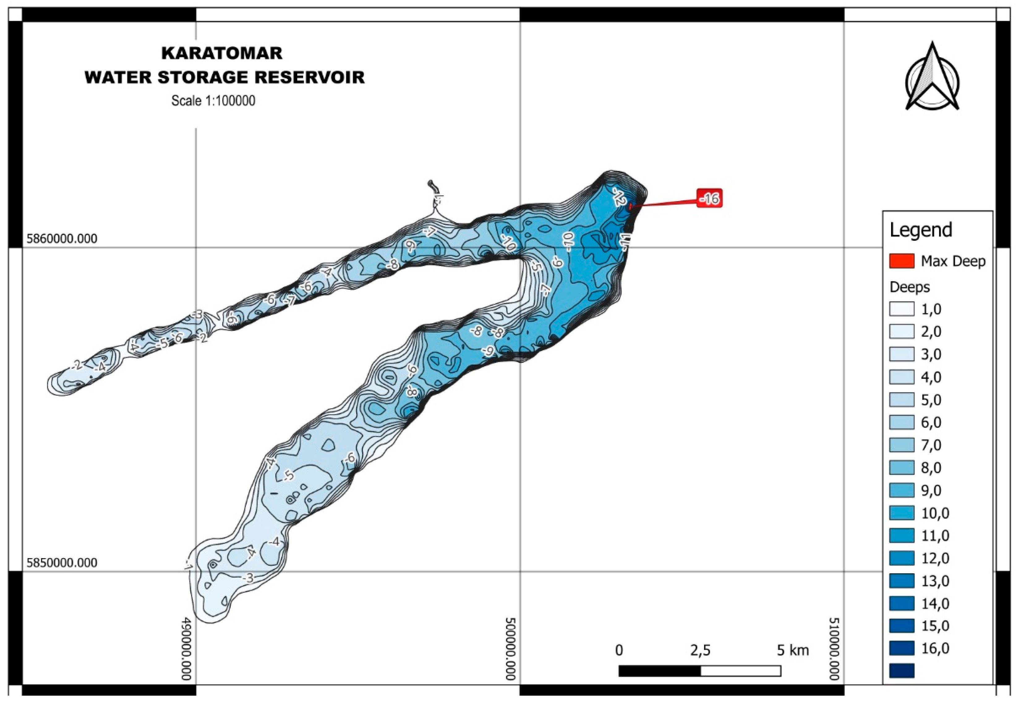
Table 1.
Main characteristics of the Apache 3 autonomous bathymetric drone.
| Parameter name | Value |
|---|---|
| Echo sounder | |
| Measured depth range, m | from 0.15 to 200 |
| Echo sounder operating frequency, kHz | 200 |
| Echo sounder resolution, m | 0.01 |
| Echo sounder beam width, ° | 6.5±1 |
| Root mean square error (RMSE) of depth measurements, m | 0.01+0.001·H, where H is the measured depth in cm |
| Location | |
| Number of channels | 624 |
| GNSS | GPS NAVSTAR: L1C/A, L1C, L2C, L2P, L5 ГЛОНАСС: L1C/A, L1P, L2C/A, L2P BeiDou: B1, B2, B3 Galileo: E1, E5A, E5B SBAS: WAAS, EGNOS, MSAS, QZSS, GAGAN |
| RMSE | RTK in plan 8.0 mm + 1.0 mm/km |
| RMSE | RTK in height 15.0 mm + 1.0 mm/km |
| RMSE DGPS in plan | 0.25 m |
| RMSE DGPS in altitude | 0.5 m |
| Heading accuracy | 0.2° per 1 m baseline |
| Inertial navigation stability | 6° per hour |
Table 2.
Comparative review of methods of bathymetric and topographic research of reservoirs based on literary sources.
Table 2.
Comparative review of methods of bathymetric and topographic research of reservoirs based on literary sources.
| Link | Name/Brief description of the method | Required equipment | Advantages | Disadvantages |
|---|---|---|---|---|
| Manual methods of depth measurement and topographic survey of the relief of the coastal zone of the reservoir | ||||
| - | The method is based on measuring the length of the released lead line from the side of the vessel. | Hand lot, vessel | Affordability of single measurements | Low speed and accuracy of water body depth measurements |
| [29] | Theodolite survey | Theodolite, steel measuring tape (or optical rangefinder) | Affordability of single measurements | Low measurement speed, Limited sizes of theodolite traverses (polygons), Difficulty of carrying out work on hard-to-reach riverbed slopes |
| Tacheometric survey | Tacheometer | |||
| Tablet survey | Measuring plate | Difficulty of carrying out work on riverbed slopes | ||
| Surface leveling (vertical or altitude survey) | Level | High precision | Need for additional planning and reference work of reference points | |
| Phototheodolite survey of coastline relief (terrestrial) | Phototheodolite | |||
| Methods of automated bathymetry and topographic survey of the relief of the coastal zone of the reservoir | ||||
| [39] | Hydroacoustic sounding of the underwater part of the reservoir | Echo sounder, underwater measurement vessel/drone, attitude sensors | Possibility of capturing large volumes of data with high accuracy | Impossibility of taking measurements on overgrown areas of the reservoir |
| [40,41] | Phototheodolite survey of the coastline relief (aerial photography) | Aircraft, aerial camera | Possibility of obtaining plans of large areas. | Need for additional planning and reference work of reference points Sensitivity of measurement accuracy to the density of vegetation cover. |
| [42] | Laser scanning of the coastline relief | LiDAR, optional aerial survey aircraft + attitude sensors |
Obtaining topographic plans of complex profiles. High accuracy. Measurement speed. |
Sensitivity of measurement quality when working with reflective surfaces |
| Methods of remote satellite sensing and digital modeling of water bodies | ||||
| [34,37] | Group of space radar altimetry methods | Requires satellite LiDAR data and field survey data to determine depth | Obtaining topographic plans of complex profiles. High accuracy. Measurement speed |
Dependent on cloudiness and weather conditions. Possibility of constructing only surface reliefs |
| [5,38] | A group of methods for reconstructing and forecasting bathymetry using space data and global models. | Space photography data is required | Possibility of constructing the full relief of a reservoir bowl | Often does not take into account the complex bathymetry of a water body |
Table 10.
Results of comparison of the main planned and current values of the Karatomar reservoir.
Table 10.
Results of comparison of the main planned and current values of the Karatomar reservoir.
| Parameters | Data 1966 | Data 2024 | Deviation |
|---|---|---|---|
| Reservoir volume, | 791 mil. m3 (when the bowl is 100% full | 367 mil. m3 (at 98% bowl filling | -53.60 % |
| Useful reservoir volume, | 562 mil. m3 | Not rated | - |
| Water surface area, | 93.7 km2 | 61.47 km2 (based on digitized polygon) ± 5.63 km2 |
-34.44 ± 6.01% |
| Maximum depth, m | 19.8 | 16.0 | -18.99 % |
Disclaimer/Publisher’s Note: The statements, opinions and data contained in all publications are solely those of the individual author(s) and contributor(s) and not of MDPI and/or the editor(s). MDPI and/or the editor(s) disclaim responsibility for any injury to people or property resulting from any ideas, methods, instructions or products referred to in the content. |
© 2025 by the authors. Licensee MDPI, Basel, Switzerland. This article is an open access article distributed under the terms and conditions of the Creative Commons Attribution (CC BY) license (http://creativecommons.org/licenses/by/4.0/).
Copyright: This open access article is published under a Creative Commons CC BY 4.0 license, which permit the free download, distribution, and reuse, provided that the author and preprint are cited in any reuse.


