
Submitted:
01 April 2025
Posted:
02 April 2025
You are already at the latest version
Abstract
The main aim in this paper is to present new analytical representations of the thermodynamic functions of finite-temperature Thomas-Fermi model. First, an algorithm to solve the nonlinear equation of the model, which starts by rewriting it as a Fredholm integral equation, is described. Application of Newton's procedure, then, yields a sequence of linear Fredholm integral equations, which are solved using the standard Nystr{\"o}m's method. Use of Brachman's equation for direct computation of thermal energy of electrons is elaborated. Using extensive tabulations of the thermodynamic functions, over a wide range of scaled temperature and scaled densities, analytical representations of electron energy, pressure, ionization, Fermi energy and initial slope of Thomas-Fermi function are developed. Accuracy of these functions is established via computation of electron-Hugoniot and the Hugoniot of Cu and comparison with experimental (or theoretical) data up to about 20.4 TPa.
Keywords:
Thomas-Fermi model
; electron equation of state
; thermodynamic properties
1. Introduction
The Thomas-Fermi (TF) model is the simplest of all orbital-free density functional theories for determining the electron-components of thermodynamic properties of materials [1,2]. Its finite-temperature generalization, together with the spherical atomic cell concept, is commonly used for computing electron-properties of hot dense matter [3]. The TF model leads to a nonlinear boundary value problem that is to be solved using numerical techniques [4]. Important improvements to the original algorithm to solve the TF equation have also been reported [5]. Addition of the quantum mechanical exchange correction to the TF model leads to Thomas-Fermi-Dirac (TFD) model, while the Thomas-Fermi-Dirac-Weizsäcker (TFDW) model is obtained when electron-density gradient corrections are accounted [6]. The quantum statistical model (QSM) belongs to the same class although its development yielded the correct coefficient of the gradient term in the energy functinal [7]. Numerical computations of electron-component of equation of state (EOS) using the QSM is somewhat involved. Moreover, there is no scaling of thermodynamic properties with atomic (Z) and mass (A) numbers [8,9]. Applications of TF model indeed demonstrate the need to account for the electron binding effects even in obtaining thermal part of electronic properties [10]. Available analytical representations [11,12] of tabulated numerical results are not sufficiently accurate in the wide density-temperature plane required for applications. Perturbation solutions starting from the hot-curve (fully ionized state) do not explicitly account for the nuclear potential in the results [13]. The excellent compilation of approximate analytical solutions of TF equation [14] reinforces the need for efficient numerical schemes.
The well known method to solve the TF equation is to rewrite it as a Voltera integral equation and thereafter formulate a discrete version and then apply the shooting method to obtain a solution [4]. However, numerical difficulties arise in the shooting method for lower temperature range, and special techniques are needed to overcome them [5]. An alternate method is to apply Newton’s method to solve the non-linear TF equation. A discrete version of the resulting (linear second order) differential equation, obtained via the finite difference method (FDM), and the double sweep method provide an efficient algorithm, as the coefficient matrix is tri-diagonal [15]. However, the second order derivative of the TF-function does not exist at the origin and is very large in its neighborhood where the FDM is not applicable. One of the aims of this paper is to develop a method with forth order accuracy to solve the linear equations which result from Newton’s method. Then, it is pointed out that Brachman’s differential equation [16] is employable as it provides directly the thermal component of electron energy. Furthermore, with the use of very accurate rational function approximations of Fermi-Dirac integrals [17], the present paper offers a simple algorithm that works in the entire scaled temperature-density plane.
The paper is organized as follows. The relevant formulas related to the TF model are collected in thomas-fermi-model, while the numerical scheme is detailed numerical-scheme. Analytical representations of thermodynamic functions, which include electron energy, pressure, ionization, Fermi energy and initial slope of TF-function, are provided and discussed in analytical-representation. Accuracy of these representations is demonstrated, in applications, via computation of electron-Hugoniot and the Hugoniot of Cu and comparison with experimental (or theoretical) data up to about 20.4 TPa pressure. Finally, summary provides a summary of the work.
2. Thomas-Fermi Model
The finite-temperature TF model follows from the Poisson equation for electrostatic potential in an atomic cell, where the electron density is given by the Fermi-Dirac distribution [3]. In scaled variables, it yields a nonlinear second order differential equation [4]
Here, the dimensionless radial co-ordinate , where R denotes the spherical cell radius. The TF-function and dimensionless parameter are defined as
where is the electrostatic potential, the Fermi energy, Boltzmann’s constant and T temperature. Note that denotes the magnitude of electronic charge so that is the electron potential energy. Remaining symbols are electron mass and Planck’s constant h. The Fermi-Dirac function of order is given by
Accurate rational function approximations [17] for these integrals (and their inverse functions) are available for and . The limiting condition that must approach the nuclear potential as yields one boundary condition . The other follows from the condition that the atomic sphere is electrically neutral, which implies that potential gradient at R. This fact, together with the choice of potential value at R (which is arbitrary) provides the condition . Now, note that which is also implicitly defined through the relation , where is number of free electrons at temperature T and the cell volume.
2.1. Thermodynamic Properties
Detailed derivations of all thermodynamic properties within the TF model are well known [4]. For instance, electron pressure is given by
Only is needed for computing P. Alternatively, if P is known, and thereafter can be obtained. Kinetic energy of electrons (per atom) needs over the full interval, and is expressed in the integral
Similarly, the potential energy of electrons is given by
Note that the last three equations (3 - 5) yield the virial theorem expressed as . A partial integration in Eq.(5) together with the TF equation and the relation yields the alternate expression
Asymptotic forms of should be used near in evaluating these integrals. An alternate way to compute total energy of electrons (per atom) is the following.
The free energy F and thereafter the entropy S are obtained [16] by integrating the Gibbs-Helmholtz equation . Entropy so obtained is given by
where and are, respectively, the electron-electron and electron-nuclear components of potential energy . Using the definition of and Poisson equation for V, it is readily found taht , where denotes the slope of TF function (with respect to x) at the origin [15]. Use of this expression, together with the virial theorem, reduces Eq.(6) to the expression . Finally, the thermodynamic relation yields Brachman’s differential equation for energy [16,18]
where the partial derivatives with T, like , are taken at constant volume. This first order differential equation can be integrated from a suitable starting value of T. Note that only , and not the full TF function , is needed in Brachman’s equation, however, the differential equation needs to be integrated.
In the high temperature limit when electron density is uniform, , and consequently, and . Fermi energy reduces to in the same limit. This limiting form yields (see Eq.(7)) the ideal gas limit , as becomes independent of T in this limit. In the zero-temperature limit [18], Eq.(7) reduces to , where is the initial slope of (the zero-temperature) TF-function, is the TF scaling length, and the Bohr radius. Substituting , and integrating the resulting equation from T to ∞, the thermal energy of electrons is obtained as
where . It is necessary to integrate from T to ∞ for the sake of numerical stability (see Eq.(20)). Further, the zero-temperature terms are subtracted in so that the integral does not diverge as . Note that the expression for is consistent with the high-temperature limits and for thermal pressure and energy of electrons in the cell. The term , arising from in this limit, cancels out. Very accurate numerical approximations for zero-temperature pressure and slope versus cell radius are available [21,22] (see analytical-representation).
3. Numerical Scheme
To develop a numerical method, the TF equation is converted to an integral equation. On integrating from x to 1, and thereafter from 0 to x, Eq.(1) reduces to
where the kernel is for and for . The boundary conditions on are incorporated in Eq.(9). To employ Newton’s method, first the non-linear term is approximated using the expansion , which follows from Taylor’s expansion of around the function . The recurrence relation is also used. Substitution into Eq.(9) yield linear equation
The known function is
The integrals in these equations exist for because and as . Several numerical schemes exist [19] for solving the linear Fredholm integral equations (FIE) as in Eq.(10). Thereafter, a few iterations, together with the replacement , provides the required solution, if Newton’s method converges.
In the Nyström’s method to solve FIE, which is employed to convert the FIE to a matrix equation [20], the integral term is evaluated using a suitable quadrature. In the procedure adapted here, (and also ) is approximated using piece-wise quadratic polynomials in the sub-intervals in [0, 1]. To this end, the interval [, 1] is divided in to N (even) sub-intervals defined with (odd) mesh points . This choice of provides more mesh points near where varies more steeply. There are only unknowns to be determined as is known. In the sub-interval (), the unknown function is represented as as a quadratic polynomial
Substitution of into Eq.(10) yields Nyström’s interpolation formula
where the modified source function is given by
The weight functions (for ) are given by
An additional set of functions are also introduced for expressing the source term as
Note that the second sum (with ★ on lower limit) involving is only over even values of j. The last integral term is obtained using the approximation . In all computations, in is approximated by the quadratic polynomial . This polynomial passes through and and has the slope at the origin. The slope at the origin given by
The first line follows by integrating Eq.(1) over [0,1]. Latest available values of and are employed in computer implementation. Rigorously, a term proportional to must be added in near to account for the divergence of . However, this is not considered here since the dominant term contributing to the integral (in ) is . All the integrals are readily evaluated using low order (say 6 or 8) Gauss quadrature. However, the asymptotic term should be subtracted within the integral in Eq.(18) (before applying Gauss quadrature formula) and its contribution added separately. Similar technique may be used in obtaining from Eq.(17) for better accuracy. The approximation leading to Eq.(13) is the same as in obtaining Simpson’s integration formula and hence the local truncation error is proportional to . The collocation rule in Nyström’s method amounts to enforcing Eq.(13) at the discrete set of values , which yields a matrix equation of order for the vector . The coefficient matrix is . The components and those of of the vectors and are and , respectively. Elements in a particular column of the lower triangular part of are the same. The upper triangular part can be written as with sharing the same property.
The number of Newton’s iterations needed for convergence to a specified accuracy is indeed depended on the starting guess solution. For illustration, Figure 1 shows needed versus to reduce the Euclidean norm between successive iterates to . The starting guess solution for each temperature corresponds to uniform electron density and are the number of sub-intervals used. The scaled cell radius in this case is , however, similar results are obtained for expanded as well as compressed configurations. Even for very low temperatures eV, Newton’s method converges in about 10 iterations to the specified accuracy. The inset in this figure is the converged profile for reduced temperature eV, which justify piece-wise quadratic polynomials used in the method. It is also found that the spatial profile of converges with about 10 sub-intervals N.
3.1. Thermodynamic Quantities
All the properties described earlier (see thermodynamic-properties) is computed using the converged solution vector . For instance, pressure is obtained directly from Eq.(3) using the converged value of . Next, the kinetic energy is obtained as
Note that the second sum is only over even values of j. The contribution of the asymptotic term in to the first integral should be accounted as explained earlier in the case of . Further, follows from the virial theorem. Alternatively, the thermal energy at temperature is obtained directly via a recursion relation
This follows directly from Eq.(8), and the dependence of and on cell volume is suppressed. For sufficiently large n, the starting value of thermal energy . An interpolation function of is first constructed from its tabulation versus T and then used in this relation. The last integral in Eq.(20) is computed with three-point Simpson’s rule. The slope is given by Eq.(18) (also see analytical-representation).
4. Analytical Representations
Using the results of extensive calculations, covering the temperature range (eV) and cell radius range (Ao), analytical representations for thermal energy , thermal pressure , thermal ionization , Fermi energy and initial slope of TF-function are derived. As explained earlier, while ionization provides Fermi energy, the initial slope gives entropy and free energy.
1. Thermal Energy
Thermal energy is represented in the form
The factor is the scale parameter for energy in TF-model and (eV) is the scaled temperature. The parameters (for ) are functions of the scaled cell radius (Ao). The expression for is proportional to the asymptotic forms and in the limits and , respectively. Therefore, it is evident that . The parameter is already determined by Gilvarry [21,22] using solutions of temperature-perturbed TF equation. It’s fit as a function of is
Here, is the pressure at zero-temperature and , and . The factor arises because should be proportional to . The dimensionless parameter is proportional scaled cell-radius as ( the Bohr radius) and are constants. The zero-temperature pressure , the boundary value of zero-temperature TF-function and the parameters and are fitted functions of given by
The remaining parameters and are fitted to the rational expressions
As application of these formulas, plots of scaled energy (eV/atom) versus scaled temperature (eV) are shown in Figure 2 for three values of scaled cell radius . Here, the symbols are numerical values and lines represent analytical representations. It is important to note that all the three curves merge together at high temperatures thereby indicating approach to ideal gas limit.
2. Thermal Pressure
The analytical representation for thermal pressure is chosen as
Here the factor is the scale parameter for pressure. Now, all the parameters () are functions of the scaled cell radius . Since the expression for is proportional to the asymptotic form in the limit , the parameter . The parameter (already determined by Gilvarry [21,22] using the temperature-perturbed TF equation) is given by
The factor arises in this expression because should be proportional to . Other quantities , and are already given above. The parameters and are represented as
Plots of (GPa) versus (eV) are shown in Figure 3 for same values of scaled cell radius . Here also the symbols denote numerical values while the lines depict analytical representations. The linear variation at high temperature in all the three curves indicates approach to ideal gas limit. Unlike the fits available in the literature [11,12], the expressions in Eq.(21) and 22 have the correct dependence on cell radius , and are applicable in compressed as well as expanded volume regions (see applications).
4. Thermal Ionization
As the numerical procedure gives , thermal ionization is directly given in terms of (see thomas-fermi-model). A numerical fit to as a function of density and temperature is given by More [23]. However, it is found that the relative error in this formula is as much as 30 percent for low temperature and expanded volume states. The data generated now is expressed in rational function representation as
This form approaches approaches Z as , and the parameter provides ionization at zero-temperature. Theoretically, the value of in the limit should approach 1; the numerical value obtained is close to this theoretical limit. Plots of versus are shown in Figure 4 for same values (0.9348, 4.339 and 20.14 ) of scaled cell radius considered earlier. Again, symbols are numerical values and lines analytical representations. The present expression has about percent accuracy in the entire plane.
Dependence of all the five parameters on is obtained as
3. Fermi Energy
Although the solution procedure of TF model directly gives , it can also be obtained in terms of ionization using the inverse of integral (see thomas-fermi-model). Since very accurate representation of this inverse function is available [17], it is unnecessary to represent directly. However, for the sake of completeness, scaled values versus scaled temperature (eV) are shown in Figure 5 for the three values (0.9348, 4.339 and 20.14 ) of scaled radius .
4. Initial Slope
The initial slope of the Thomas-Fermi function is needed in calculating entropy (and free energy) as it is defined by . To this end, the parameter is introduced so that entropy is expressed in terms of thermal quantities as . The representation chosen is
Here, is the limiting form of corresponding to uniform distribution of electrons. This follows readily from . Further, is the limiting value of as . This separation is useful as as . The representation for , where is computed using ionization , is given by
where and are in eV and Ao, respectively. The parameters () and the zero-temperature slope are found to be
The variation of versus is shown in Figure 6 for three different values (0.9348, 4.339 and 20.14 ) of . The chosen functions represent the data accurately. For the sake of completeness, the dependence of versus is shown in the inset in this figure.
The definition of and Eq.(8) shows that is the same as . The fit for (initial slope of zero-temperature TF-function) provided by Gilvarry [21,22] is
with . Note that is the slope for isolated atom. This yields as the energy of the isolated atom at zero-temperature. Numerical results show that the two representations for agree well.
5. Applications
A three-component description of the EOS [24,25] employs the zero-temperature isotherms , the ionic components of thermal energy and pressure and the electron components . Usually, the electron components are obtained as interpolated data from large tables [24]. For applications that do not involve very high temperatures, empirical fits [11,12] of the data published by Later [4] are also employed. These fit are interpolation functions between low-temperature electron properties (as in Fermi-gas model) and the ideal gas model. The representations provided in this work (see analytical-representation) offers an alternate procedure which provides results close to that obtainable from data tables.
5.1. Electron Hugoniot
The principal Hugoniot of only electrons within the Fermi-gas model is well known [26]. Considering a point nuclear charge at the cell center, together with the analytical representations of and , the electron-Hugoniot is easily computed. In the results shown in Figure 7, pressure ratio is shown versus the compression factor . Curve-1 corresponding to TF model shows that the maximum compression obtainable is . This figure also contains the results obtained using the empirical fits [11,12] mentioned above. The maximum compression of is found with the fits because of the absence of any binding effect of electrons in the cell. The inset in this figure shows reduced specific heat (per electron) for cell radius . The peak found in around K is due to electron binding to the nucleus.
5.2. Hugoniot of Cu
For application to Cu, Vinet’s zero-temperature isotherm [27,28] given by is employed. The corresponding analytical expression for energy follows from the relation and . Here , and are, respectively, the bulk modulus, its pressure derivative and cohesive energy (per gram) at volume . This volume is determined such that total pressure (including those of ions and electrons) is GPa at ambient temperature (300 K) and volume . These formulas are suitably corrected using QSM [7,8] at very high pressures. Pressure within QSM is analytically expressed as (ℏ is reduced Planck’s constant, m electron-mass and the Bohr radius). The quantity (electron density at the atomic cell surface) is given by where and (R denotes cell radius). Energy in QSM also follows from the relation . An interpolation procedure [29] to smoothly go over from Vinet’s model to QSM uses an adjustable volume such that the corrected pressure and for . These for smaller volumes are obtained by imposing continuity of and its first two derivatives at . Note that the definition ensures that is continuous at [30].
Ionic thermal contributions are obtained using Johnson’s model [31] wherein the thermal ionic energy (per gram) and pressure are expressed as and . Here, Debye model provides the EOS in solid phase. The components and (non-zero for , the melting temperature) accounts for changes in energy due to melting, heat of fusion and subsequent approach to ideal gas behavior [25,31]. A three-term fit [32] to the Grüneisen parameters is employed in the present application.
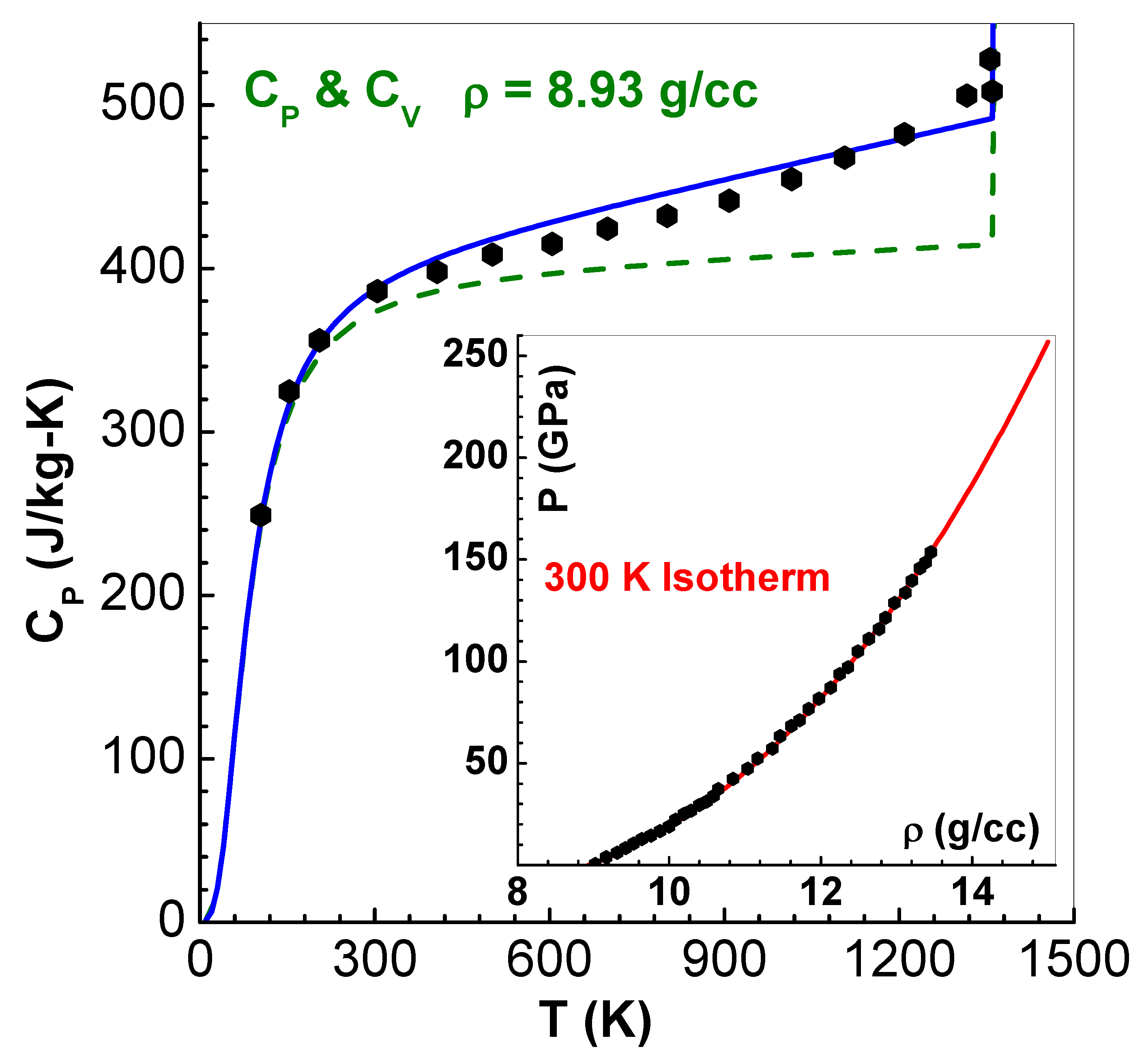
The principal Hugoniot and zero-temperature isotherm are compared with available experimental (also theoretical) data [33] in Figure 8. The Hugoniot agrees very well over an extended range of pressures up to TPa. The zero-temperature isotherm is compared over a larger range up to 100 TPa pressure in the insert. Improvements to due to the corrections using QSM (with ) are also shown here. To check the ionic thermal model, the constant-pressure specific heat in the solid phase at is compared with reported results [33] in Figure 9. This figure also depicts by the dashed line. Results agree well in spite of the simplicity of the ionic model. The sharp increase in and at K occurs due to the addition of heat of fusion. The room-temperature (300 K) isotherm shown in the inset agrees excellently.
6. Summary
An efficient numerical algorithm based on Newton’s method to solve the TF equation is developed in this paper. The basic idea in the method, which rewrites the TF equation as a non-linear Fredholm integral equation, circumvents some of the pitfalls in earlier work using FDM. Results presented show that Newton’s iterations converge within few iterations in the whole temperature-density plane. Furthermore, the algorithm needs small number of sub-intervals for discrete approximations. The use of Brachman’s equation for direct calculation of electron-thermal energy is elaborated. Analytical representations of thermodynamic quantities are obtained from extensive tables of data obtained with the present method. These include thermal energy, pressure, ionization, Fermi energy and initial slope of TF-function (which is needed for entropy and free energy). Accuracy of the representations is ascertained via computation of the electron Hugoniot and principal Hugoniot of Cu and comparison with experimental (or theoretical) data. The present paper significantly extends to all temperatures the earlier work (restricted to low temperatures) of Gilvarry on the TF model.
References
- Thomas, L. H. The calculation of atomic fields. Proc. Cambridge Phil. Soc. 1927, 23, 542. [Google Scholar] [CrossRef]
- Fermi, E. A statistical method of determining some properties of the atom and applying it to the theory of the periodic table of elements. Z. Physik 1928, 48, 73. [Google Scholar] [CrossRef]
- R.P. Feynman, N. Metropolis ans E. Teller. Equation of state of elements based on the generalized Fermi-Thomas theory. Phys. Rev. 1949; 75, 1561.
- Latter, R. Thermal behavior of Thomas-Fermi statistical model of atoms. Phys. Rev. 1955, 99, 1854. [Google Scholar] [CrossRef]
- Shemyakin, O. P.; Levashov, P. R.; Obruchkova, L. R.; Khishchenko, K. V. Thermal contribution to thermodynamic functions in the Thomas-Fermi model. J. Phys. A: Math. Theor. 2010, 43, 335003. [Google Scholar] [CrossRef]
- Perrot, F. Zero-temperature equation of state of metals in the statistical model with density gradient correction. Physica 1979, A 98, 555. [Google Scholar] [CrossRef]
- Kalitkin, N. N.; Kuz’mina, L. V. Curves of cold compression at high pressures. Sov. Phys. Solid State 1972, 13, 1938. [Google Scholar]
- More, R. M. Quantum-statistical model for high-density matter. Phys. Rev. 1979, A 19, 1234. [Google Scholar] [CrossRef]
- Perrot, F. Gradient correction to the statistical electronic free energy at nonzero temperatures: Application to equation-of-state calculations. Phys. Rev. 1979, A 20, 586. [Google Scholar] [CrossRef]
- Shemyakin, O. P.; Levashov, P. R.; Khishchenko, K. V. Equation of state of Al based on the Thomas-Fermi model Contrib. Plasma Phys. 2012, 52, 37. [Google Scholar]
- Kormer, S. B.; Funtikov, A. I.; Urlin, V. D.; Kolesnikova, A. N. Dynamic compression of porous metals and equation of state with variable specific heat at high temperatures. Sov. Phys. JETP 1962, 15, 477. [Google Scholar]
- McCloskey, D. J. An Analytic Formulation of Equations of State. Memorandum RM-3905-PR; RAND corporation, Santa Monica, California, USA 1964.
- Baker, G. A ; Johnson, J. D. General structure of the Thomas-Fermi equation of state. Phys. Rev. 1991; 44, 2271. [Google Scholar]
- Pert, G. J. Approximations for the rapid evaluation of the Thomas-Fermi equation. J. Phys. B: At. Mol. Opt. Phys. 1999, 32, 272. [Google Scholar] [CrossRef]
- Nikiforov, A. F.; Novikov, V. G.; Uvarov, V. B. Quantum-statistical models of hot dense matter: Methods for computation of opacity and equation of state. In Progress in Mathematical Physics, volume 37, Eds: De Monvel, A.B. ; Kaiser, G. Birkhäuser Verlag, Basel, Switzerland, 2005.
- Brachman, M. Thermodynamic functions on the generalized Fermi-Thomas theory. Phys. Rev. 1951, 84, 1263. [Google Scholar] [CrossRef]
- Antia, H. M. Rational function approximations for Fermi-Dirac integrals. Astrophys. J. Suppl. Series 1993, 84, 101. [Google Scholar] [CrossRef]
- Gilvarry, J. J. Thermodynamics of the Thomas-Fermi atom at low temperature. Phys. Rev. 1954, 96, 934. [Google Scholar] [CrossRef]
- K. E. Atkinson, The numerical solution of integral equations on the second kind Cambridge University Press, Cambridge. 2009.
- K. E. Atkinson, L. F. Shampine, Algorithm 876: Solving Fredholm integral equations of the second kind in Matlab. ACM Trans. Math. Software 2008, 34, 1. [CrossRef]
- Gilvarry, J. J.; March, N. H. Asymptotic solution of the Thomas-Fermi equation for large atom radius. Phys. Rev. 1958, 112, 140. [Google Scholar] [CrossRef]
- Gilvarry, J. J. Thermodynamic functions in the Thomas-fermi atom model. J. Chem. Phys. 1969, 51, 934. [Google Scholar] [CrossRef]
- More, R. M. Pressure Ionization, Resonances, and the Continuity of Bound and Free States. In Advances in Atomic and Molecular Physics, Academic Press, INC. San Diego, USA 1985, 21, 305.
- More R M, Warren K H, Young D A and Zimmerman G B. A new quotidian equation of state (QEOS) for hot dense matter. Phys. Fluid 1988, 31, 3059. [Google Scholar] [CrossRef]
- Menon S V G and Nayak, B. An Equation of State for Metals at High Temperature and Pressure in Compressed and Expanded Volume Regions Condens. Condens. Matter, MDPI 2019, 4, 71. [Google Scholar] [CrossRef]
- Nellis, W. J. Shock compression of a free-electron gas J. Appl. Phys. 2003, 94, 272. [Google Scholar] [CrossRef]
- Vinet P, Smith J R, Ferrante J and Rose J H. Temperature effects on the universal equation of state of solids. Phys. Rev. B 1987, 35, 1945. [Google Scholar] [CrossRef] [PubMed]
- Vinet P, Rose J R, Ferrante J and Smith J R. Universal equation of state for solids. J. Phys: Cond. Matter 1989, 1, 1941.
- Kerley G I User’s Manual for PANDA II- A computer code for calculating equation of state SAND88-229.UC-405 1991.
- Menon S V G Convergence of Coupling-Parameter Expansion-Based Solutions to Ornstein–Zernike Equation in Liquid State Theory Condensed Matter (MDPI)2021, 6, 6.
- Johnson J, D. A generic model for the ionic contribution to the equation of state. High Pressure Research 1991, 6, 277. [Google Scholar] [CrossRef]
- Burakovsky L and Preston D, L. Analytic model of the Grüneisen parameter for all densities. J. Phys. and Chem.of Solids 2004, 65, 1581. [Google Scholar] [CrossRef]
- Peterson J H, Honnell K G, Greeff C, Johnson J D, Boettger J, and Crockett S. Global equation of state for copper AIP Conference Proceedings 1426, 1426, 763.
Figure 1.
Number of iterations (stars) versus scaled temperature , to reduce the Euclidean norm between successive iterates to , for the cell radius . The inset shows versus x for the same cell radius, but temperature eV
Figure 1.
Number of iterations (stars) versus scaled temperature , to reduce the Euclidean norm between successive iterates to , for the cell radius . The inset shows versus x for the same cell radius, but temperature eV
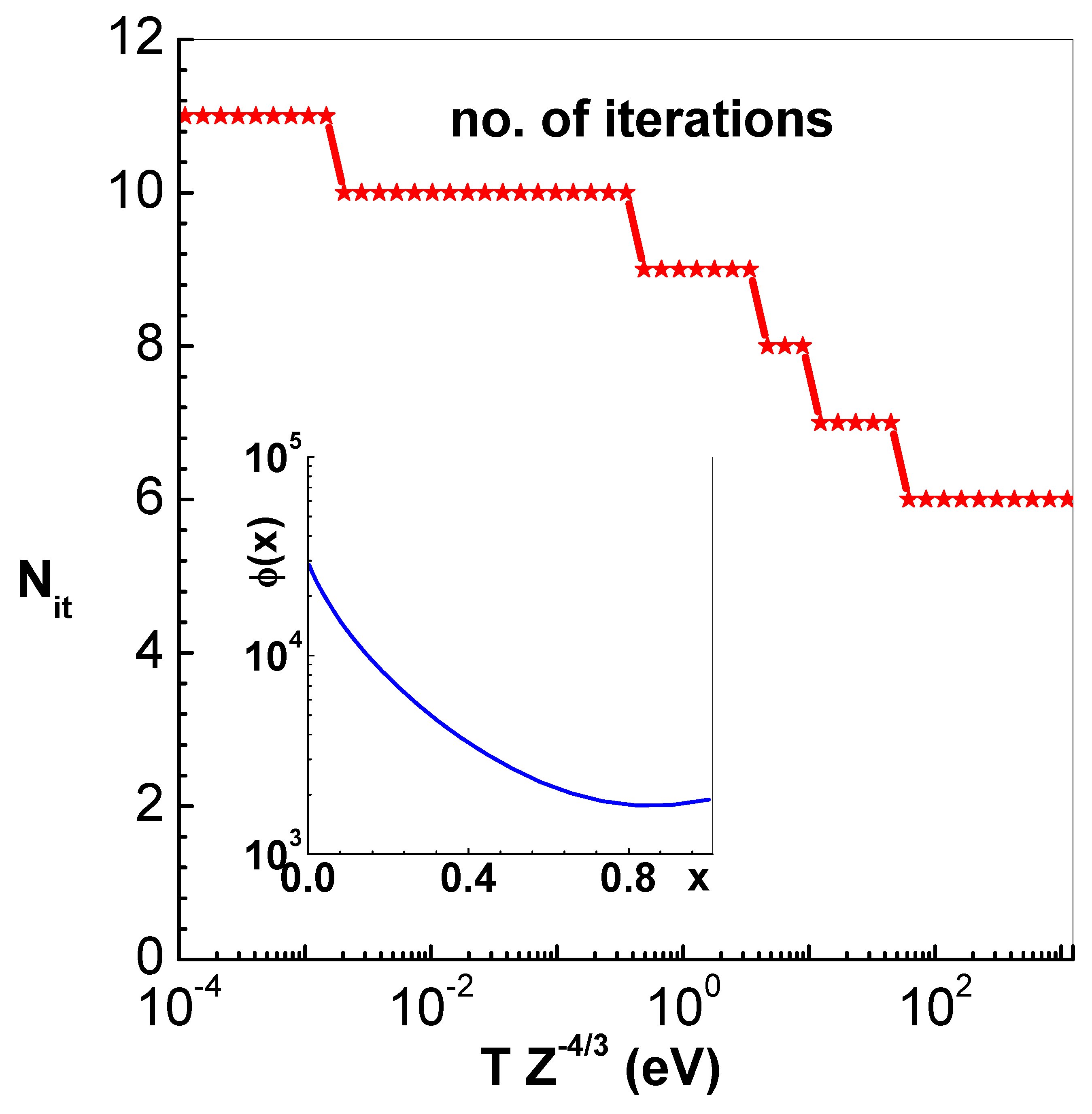
Figure 2.
Scaled energy (eV/atom) versus scaled temperature (eV) for three values of scaled cell radii . Curve-1 is for , Curve-2 for and Curve-3 for . The symbols are results of numerical solutions of TF equation while lines are from the analytical representations outlined in the text (see analytical-representation and Eq.(21))
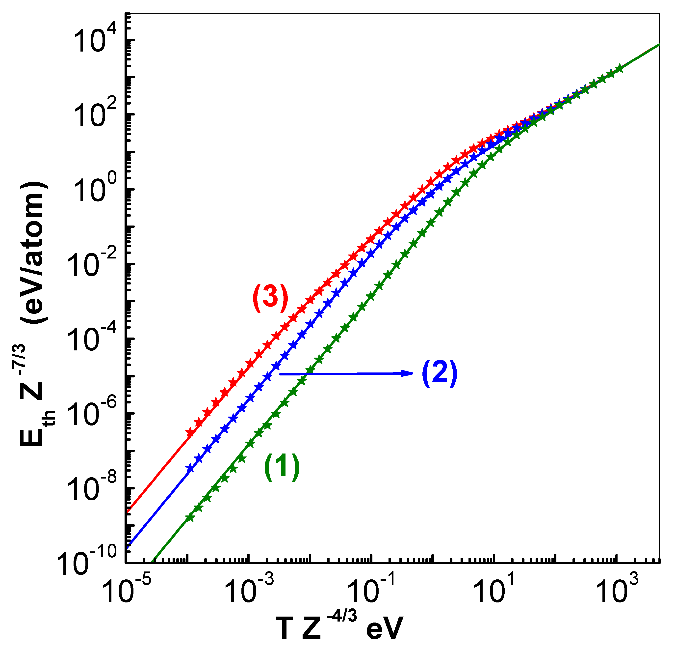
Figure 3.
Scaled energy (GPa) versus scaled temperature (eV) for three values of scaled cell-radii . Curve-1 is for , Curve-2 for and Curve-3 for . The symbols are results of numerical solutions of TF equation while lines are from the analytical representations outlined in the text (see analytical-representation and Eq.(22)).
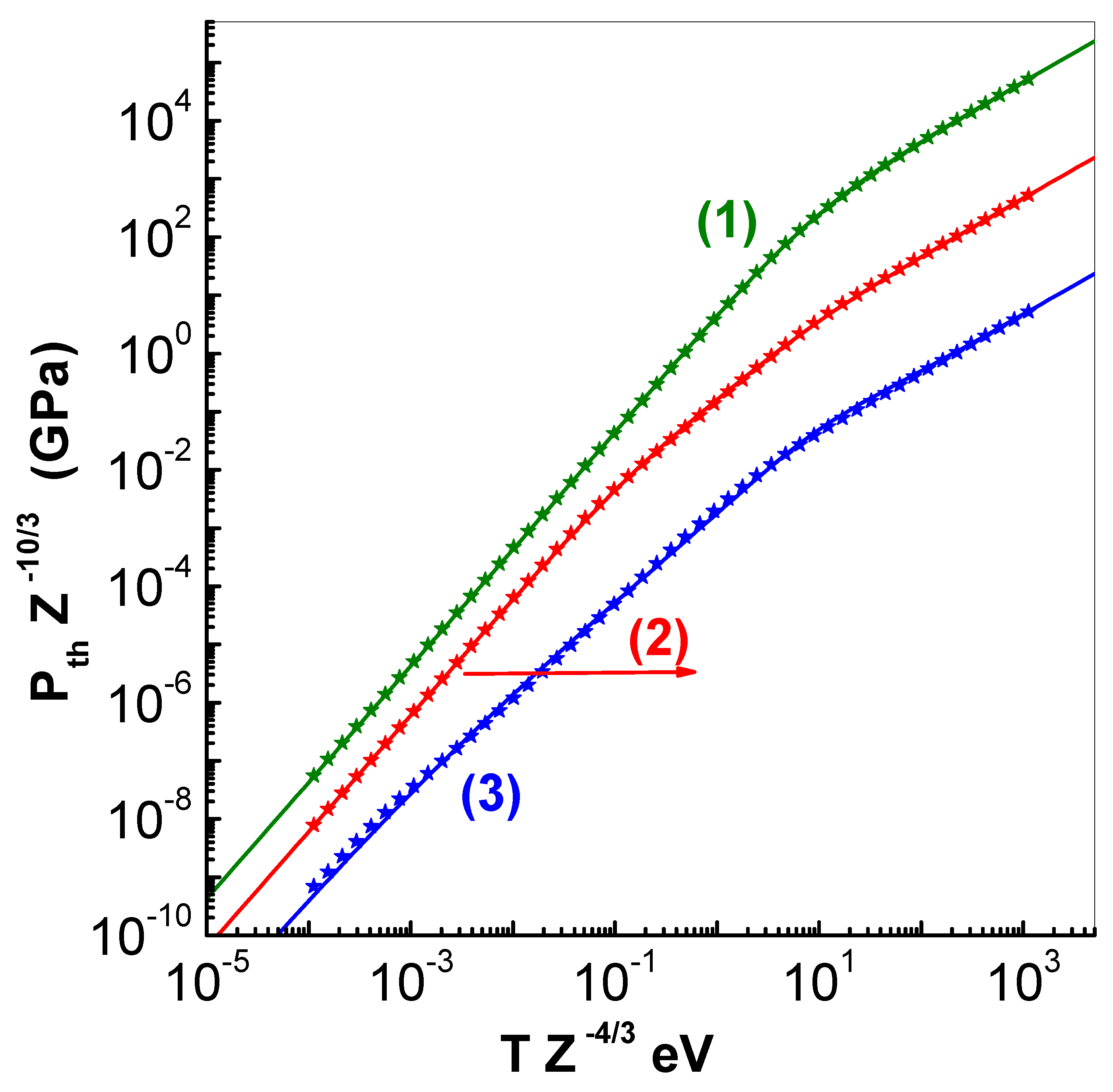
Figure 4.
Scaled ionization versus scaled temperature (eV) for three values of scaled cell radii . Curve-1 is for , Curve-2 for and Curve-3 for . The symbols are results of numerical solutions of TF equation while lines are from the analytical representations outlined in the text (see analytical-representation and Eq.(23)).

Figure 5.
Scaled Fermi energy (eV) versus scaled temperature (eV) for three values of scaled cell-radii . Curve-1 is for , Curve-2 for and Curve-3 for . The symbols are results of numerical solutions of TF equation while lines indicate their smooth variation (see thomas-fermi-model and analytical-representation and Eq.(23)).

Figure 6.
Scaled initial slope versus scaled temperature (eV) for three values of scaled cell radii . Curve-1 is for , Curve-2 for and Curve-3 for . The symbols are results of numerical solutions of TF equation while lines are from the analytical representations outlined in the text (see analytical-representation and Eq.(24)). The inset shows which corresponds to zero-temperature.
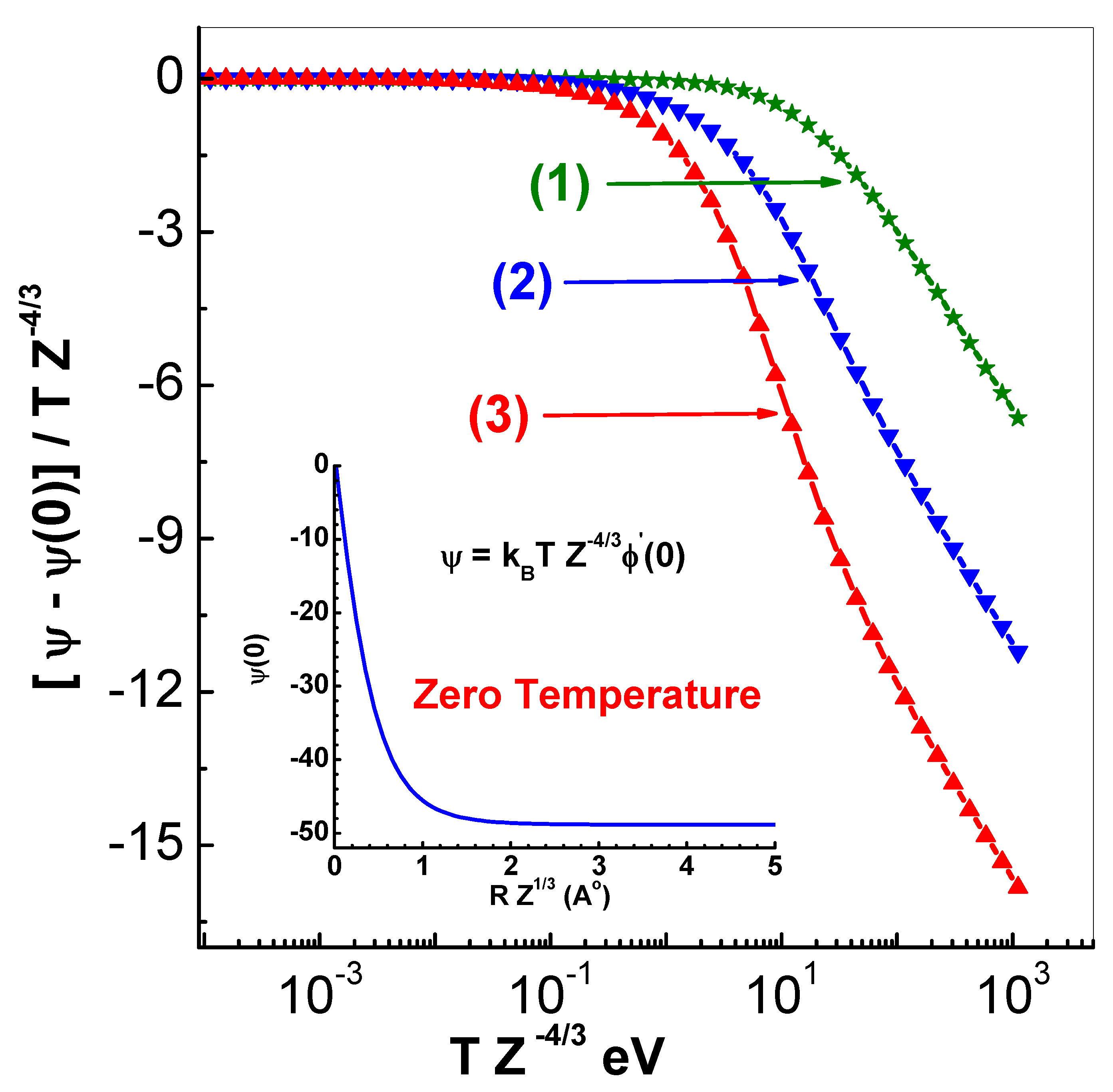
Figure 7.
Hugoniot of electrons is plotted as versus compression factor . Curve-1 corresponds to results of TF model (see analytical-representation) while curve-2 to McCloskey’s fit [11,12], which is close to Fermi gas model. The insert shows electron specific heat (per electron) for cell-radius .
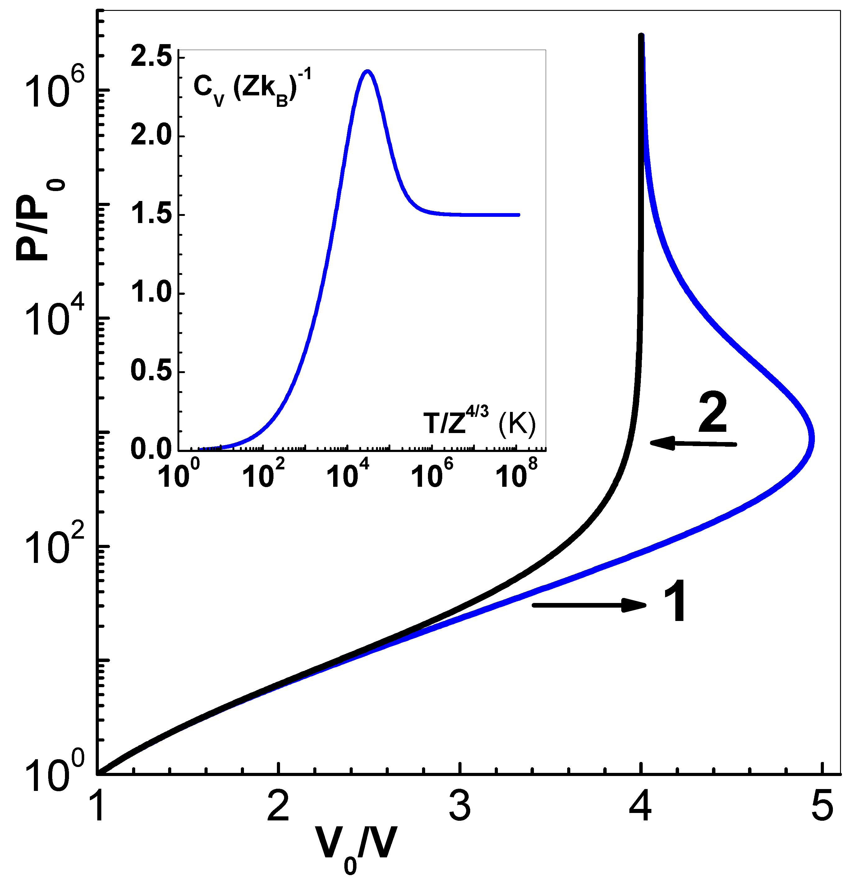
Figure 8.
Theoretical results (solid line) for principal Hugoniot of Cu are compared with experimental data (filled circles) [33] up to about 20.4 TPa. The inset shows corrected (with QSM) zero-temperature isotherm (curve-1) and also Vinet’s isotherm (curve-2); the correction is applied for .
Figure 8.
Theoretical results (solid line) for principal Hugoniot of Cu are compared with experimental data (filled circles) [33] up to about 20.4 TPa. The inset shows corrected (with QSM) zero-temperature isotherm (curve-1) and also Vinet’s isotherm (curve-2); the correction is applied for .
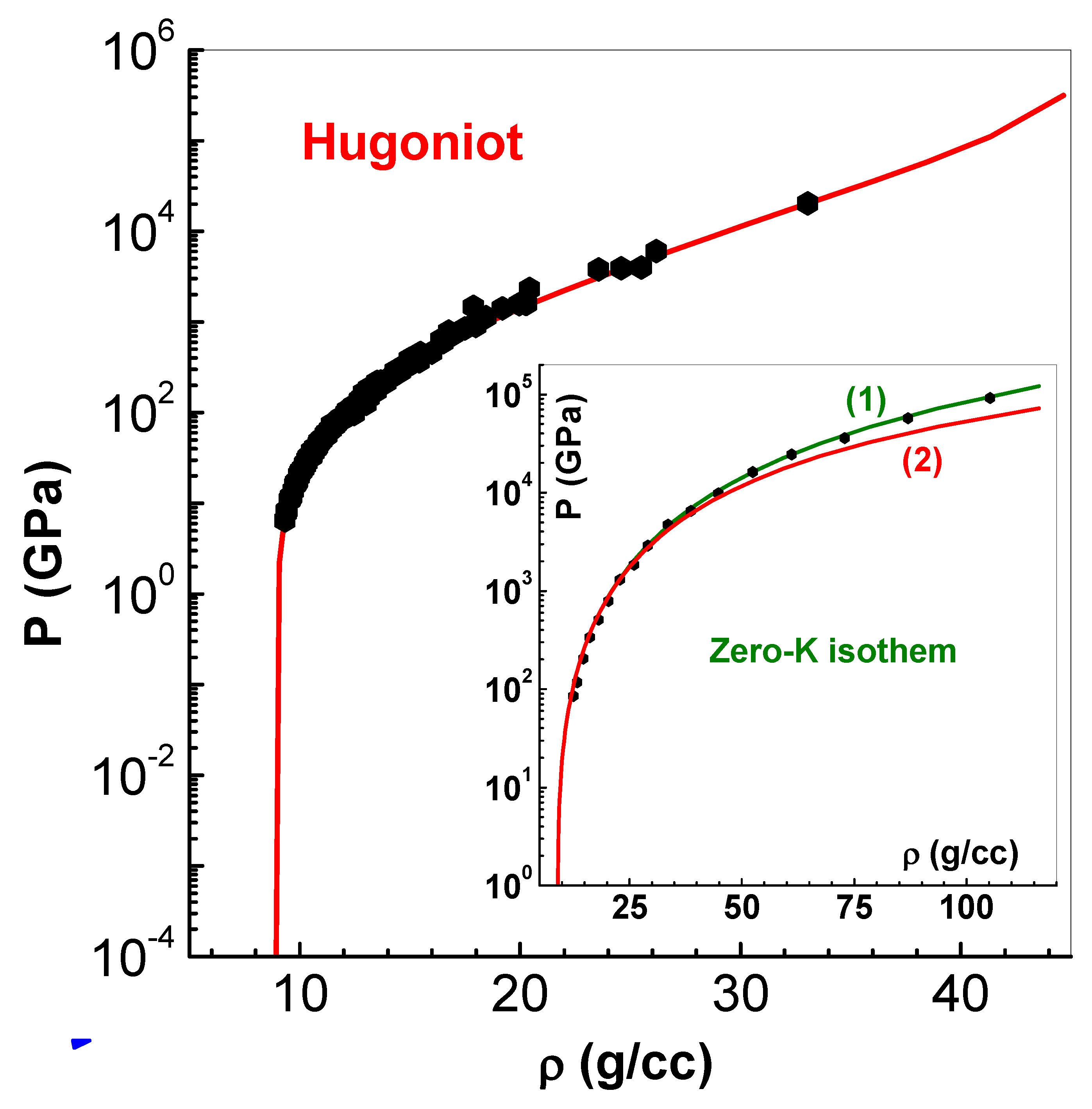
Figure 9.
Theoretical results of ionic thermal model (solid line) for constant-pressure at are compared with experimental data (filled circles) [33] in the solid phase. Computed results of are shown by dashed line. The sharp increase at K is due to heat of fusion. The room-temperature isotherm (300 K) (solid line) is compared with data (filled circles) in inset.
Disclaimer/Publisher’s Note: The statements, opinions and data contained in all publications are solely those of the individual author(s) and contributor(s) and not of MDPI and/or the editor(s). MDPI and/or the editor(s) disclaim responsibility for any injury to people or property resulting from any ideas, methods, instructions or products referred to in the content. |
© 2025 by the authors. Licensee MDPI, Basel, Switzerland. This article is an open access article distributed under the terms and conditions of the Creative Commons Attribution (CC BY) license (http://creativecommons.org/licenses/by/4.0/).
Copyright: This open access article is published under a Creative Commons CC BY 4.0 license, which permit the free download, distribution, and reuse, provided that the author and preprint are cited in any reuse.


