PyCIAT: A Configurable Python Framework for Scalable, Multi-Model Assessment of Climate Change Impacts and Adaptations in Agriculture

1. Introduction

Understanding the multifaceted impacts of climate change on agricultural production represents a critical scientific undertaking, deeply connected to global food security and sustainability goals [2,3,4]. A growing body of research highlights the significant vulnerability of diverse agricultural systems to shifts in temperature, precipitation, and extreme events [e.g., 5], underscoring the urgent need for robust assessment tools to inform mitigation and adaptation planning [2]. Process-based crop simulation models (PSMs), exemplified by widely used platforms such as DSSAT [6], APSIM [7], and STICS [8], serve as essential instruments in this endeavor. These models integrate complex biophysical processes to simulate crop growth, development, and yield responses to dynamic environmental conditions and specific management interventions. Consequently, they provide a means to quantitatively explore potential agricultural futures under various climate projections, typically derived from coordinated experiments like the Coupled Model Intercomparison Project Phase 6 (CMIP6) [9] or the Coordinated Regional Climate Downscaling Experiment (CORDEX) [10].

Despite the power of PSMs, their application in comprehensive regional or global climate impact studies involves considerable methodological complexity. Researchers are faced with the challenge of managing and processing terabyte-scale climate datasets, integrating often disparate soil and geospatial information across varied landscapes, and configuring simulations that span numerous dimensions: locations, climate models, emission scenarios, time horizons, crop varieties, management practices (including potentially complex integrated technology packages aimed at enhancing resilience and profitability [11,12]), and the PSMs themselves [13,14]. Effectively addressing the inherent uncertainties that pervade this cascade – from climate projections through to model parameterization and structure – mandates the use of multi-model ensembles (MMEs) [15,16]. Furthermore, a rigorous evaluation of adaptation measures necessitates systematic comparisons against baseline trajectories under corresponding future climate scenarios.

The practical execution of such multi-dimensional assessments frequently defaults to the creation of study-specific, often intricate scripting solutions. While capable of delivering results for a given project, this ad-hoc methodology often presents significant barriers to reproducibility, limits the ease of scaling simulations to larger domains or finer resolutions, hinders code maintainability, and makes adaptation to new models or data sources a non-trivial task [17]. The computational demands of large MME studies invariably require access to High-Performance Computing (HPC) resources. However, efficiently deploying and managing these complex, multi-stage simulation workflows within typical HPC batch-scheduling environments remains a persistent operational challenge for many agricultural modeling groups [18].

To address these methodological gaps, we have developed PyCIAT (Python Climate Impact and Adaptation Toolkit for Agriculture), an open-source, integrated framework designed to standardize and automate the workflow for agricultural climate change impact and adaptation assessments (available at https://github.com/prakau/PyCIAT). PyCIAT leverages a modular Python architecture, driven by a user-friendly YAML configuration file, to orchestrate the entire process from data preparation to analysis. It explicitly supports multi-model ensembles through standardized interfaces, facilitates parallel execution on both local machines and HPC clusters, and promotes reproducibility through its configuration-centric design. This paper details the architecture, workflow, components, and capabilities of the PyCIAT framework, presenting it as a methodological advancement for conducting scalable, reproducible, and comprehensive agricultural modeling studies under climate change.

2. Framework Architecture and Workflow

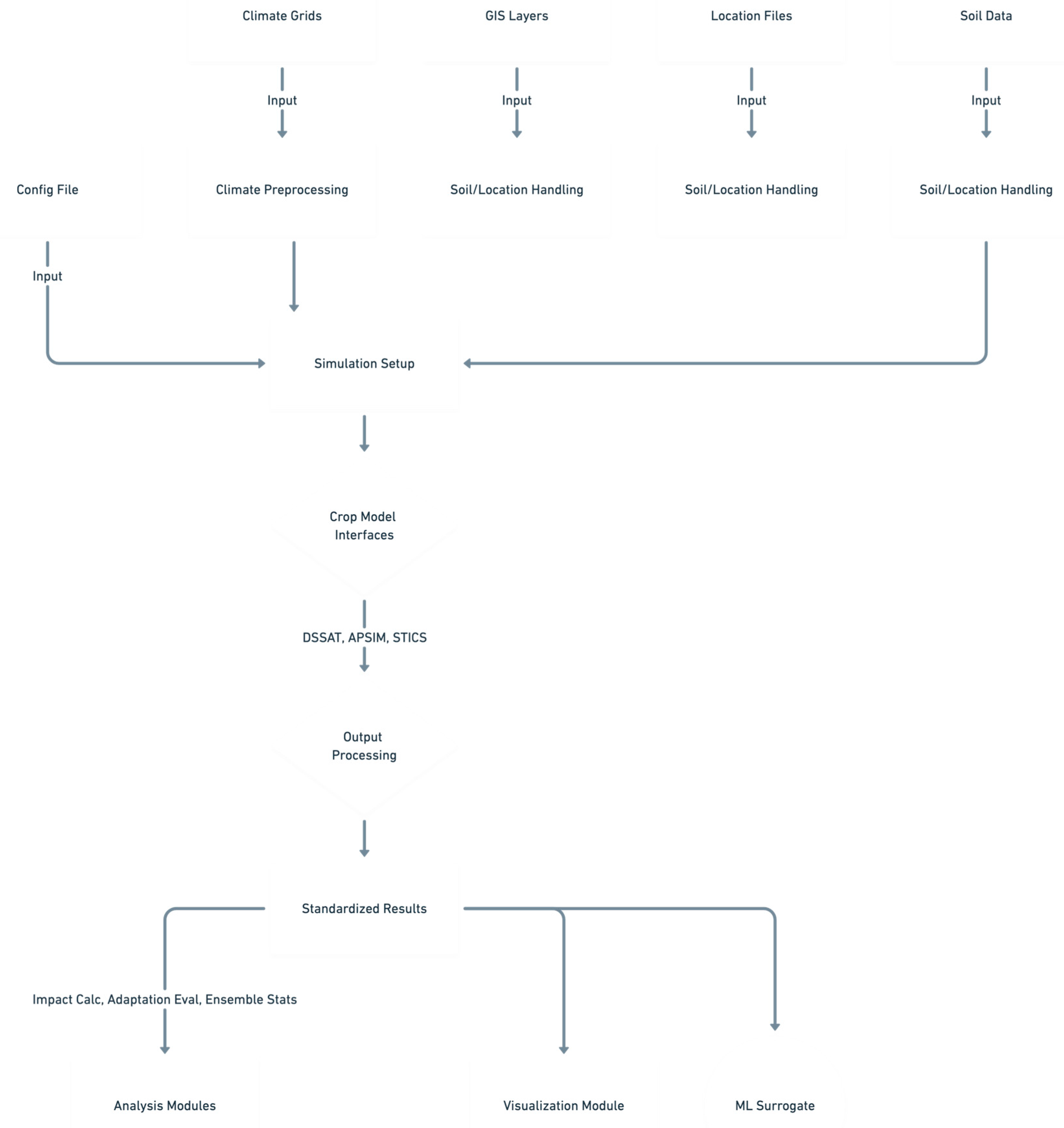
PyCIAT is architected as a modular pipeline, comprising discrete stages implemented as individual Python scripts. This structure facilitates independent execution of pipeline segments and promotes code clarity. A central YAML configuration file serves as the primary control mechanism, defining all parameters for a given assessment run. This separation of configuration from code enhances flexibility and reproducibility (Figure 1).

2.1. Configuration-Driven Control

The operational behavior of PyCIAT is dictated by the config.yaml file. Users define the entire experimental design and processing parameters within this YAML structure, covering aspects such as:

• Project Setup: Metadata, root directory paths.
• Data Sources: Paths and metadata for climate model outputs (GCM/RCM), soil profile databases, GIS shapefiles (e.g., administrative boundaries, soil maps), and location coordinate files.
• Computational Settings: Logging levels, number of parallel workers for local execution, flags and environment variable names for HPC job array integration.
• Climate Parameters: Active climate data sources, specific GCMs/RCMs and emission scenarios (e.g., SSPs) to include, target variables, reference and future time periods, spatial domain for subsetting, unit conversion specifications.
• Crop Model Selection: List of PSMs to run in the ensemble, paths to their executables, required model-specific inputs (e.g., module names, default cultivar IDs), and specification of expected output files for parsing.
• Simulation Design: Target simulation locations, baseline management practices (default sowing rules, fertilization, irrigation regimes).
• Adaptation Scenarios: Definitions of alternative management strategies or genetic traits, specifying parameter overrides relative to the baseline (e.g., earlier sowing dates, drought-tolerant cultivar ID, modified irrigation thresholds).
• Analysis Specification: List of standard output variables for analysis, the mapping rules from model-specific outputs to these standard names, definition of the baseline period for comparison.
• Optional Modules: Flags to enable/disable and configure parameters for advanced simulation options (biotic stress, soil carbon, HYDRUS) or the machine learning surrogate component.

This approach ensures that the entire experimental setup is explicitly documented within a single file, greatly aiding reproducibility and allowing straightforward modification for sensitivity analyses or new experiments. Input validation against a predefined schema (e.g., using Pydantic) is recommended as a preliminary check within the workflow.

2.2. Modular Pipeline Stages

The assessment proceeds through a sequence of command-line Python scripts, each corresponding to a logical stage of the workflow:

• 00_setup_environment.py: Initializes the run by validating the config.yaml file, resolving all configured paths (relative to a defined base_dir or current working directory), checking for the existence of essential input files and specified crop model executables, and creating the required directory structure for outputs, logs, and intermediate simulation files.
• 01_prepare_climate_data.py: Handles the ingestion and preparation of climate data. It identifies relevant climate files based on the configuration (source, model, scenario, period), loads them (typically NetCDF) using xarray [24] (optionally leveraging dask [25] for parallel I/O and processing), performs spatial and temporal subsetting, selects required variables, executes necessary unit conversions (e.g., K to °C, flux rates to daily amounts), potentially renames variables to internal standards, and extracts point-based time series for each simulation location defined in the locations file. These extracted time series are cached (e.g., as Parquet files) to avoid redundant processing in subsequent steps. Optionally, it can compute derived climate indices (e.g., heat stress days, drought metrics) if the calculation logic is implemented within src/climate_processing.py.
• 02_setup_simulations.py: Orchestrates the generation of all necessary input files for each individual crop model simulation run. It iterates through the complete factorial combination of configured factors (location, climate projection, crop model, adaptation strategy, sowing date, etc.). For each unique combination (sim_id), it retrieves the corresponding cached climate data, fetches the relevant soil profile information (potentially performing a GIS lookup using geopandas [28] if needed via src/soil_processing.py), collates the specific management parameters by merging baseline settings with adaptation overrides, and then invokes the appropriate functions (generate_weather, generate_soil, generate_experiment) within the designated crop model interface module (src/crop_model_interface/) to create all files required by that model in its specific format within a dedicated simulation directory (simulations/setup/.../sim_id/). This stage also initializes or updates a central simulation status tracking file (e.g., simulations/simulation_status.csv or an SQLite database) marking newly prepared simulations as ready for execution (e.g., READY_TO_RUN).
• 03_run_simulations_parallel.py: Executes the crop model simulations identified as READY_TO_RUN in the status tracker. It manages parallel execution using Python's multiprocessing module for local runs (respecting num_workers in config) or, if configured for HPC use, distributes the simulation tasks across nodes within a job array by interpreting environment variables set by the scheduler (e.g., SLURM_ARRAY_TASK_ID, SLURM_ARRAY_TASK_COUNT). For each simulation task, it navigates to the appropriate working directory and invokes the run_model function from the corresponding crop model interface, passing the experiment filename and executable path. Upon model completion (or failure), it captures the exit status and any relevant messages returned by the interface and updates the central status tracker (e.g., to SUCCESS or RUN_ERROR), using file locking or atomic operations to ensure safe concurrent updates.
• 04_process_outputs.py: Handles the post-simulation data extraction and standardization. It identifies simulations marked as SUCCESS in the status tracker. For each, it calls the parse_output function of the relevant model interface, providing the simulation's working directory and the configuration specifying which output files to read. The interface returns a dictionary of parsed results. This script then applies the variable mapping rules (defined in config.yaml) via src/analysis.py to translate model-native output variable names (e.g., DSSAT's GWAD) into predefined standard names (e.g., Yield_kg_ha). If optional modules like HYDRUS or biotic stress simulation were enabled and implemented, their outputs are integrated or post-processing effects applied at this stage. Finally, it aggregates the standardized results and associated run metadata (location, climate scenario, adaptation, etc.) from all successfully processed simulations into a single consolidated dataset, typically saved in Parquet format for efficient downstream analysis (analysis_outputs/combined_results_std_vars.parquet). The status tracker is updated accordingly (e.g., to OUTPUT_PARSED or OUTPUT_ERROR).
• 05_analyze_impacts.py: Performs the core climate change impact analysis using the consolidated, standardized results from Step 04. It focuses on the subset of simulations run using the 'baseline' adaptation strategy. Key operations, implemented in src/analysis.py, include: calculating baseline statistics (e.g., mean yield, phenological dates) averaged over the historical reference period for each relevant grouping (location, sowing date, crop model); calculating future changes (both absolute differences and percentage changes) for various output variables relative to these calculated baselines for different future periods and scenarios; and computing ensemble statistics (e.g., mean, median, standard deviation, percentiles like p10 and p90) across the dimensions defined as ensemble members (typically GCM/RCM and/or PSM). Results are saved as CSV or other tabular formats in the analysis_outputs/ directory.
• 06_analyze_adaptations.py: Evaluates the effectiveness of the configured adaptation strategies. It compares the projected climate change impacts (i.e., the changes calculated in Step 05 or recalculated here across all adaptations) under each adaptation scenario against the impacts projected for the baseline adaptation scenario within the same future climate context (location, climate projection, period, etc.). The 'effectiveness' is typically calculated as the difference in the projected change (e.g., Effectiveness = Change_with_Adaptation - Change_with_Baseline). Functions in src/analysis.py perform these comparisons and can calculate ensemble statistics across adaptation effectiveness metrics. Results are saved to analysis_outputs/.
• 07_generate_visualizations.py: Creates graphical outputs based on the results generated in Steps 05 and 06. Using functions defined in src/visualization.py, which leverage libraries like matplotlib [26] and seaborn [27], it can produce various plot types: time series showing ensemble mean impacts and uncertainty ranges over future periods; box plots illustrating the distribution of impacts across ensemble members; bar charts comparing the effectiveness of different adaptation strategies; and spatial maps (using geopandas [28]) visualizing the geographic distribution of impacts or adaptation benefits, potentially aggregated to administrative boundaries. Figures are saved to the figures/ directory.
• 08_train_surrogate.py, 09_predict_surrogate.py (Optional): These scripts manage the machine learning surrogate modeling component. 08_train_surrogate.py uses the consolidated simulation database (combined_results_std_vars.parquet) as training data. It applies feature engineering (e.g., creating climate indices from daily data, encoding categorical inputs like GCM name or soil type), trains a specified ML model (e.g., Random Forest, configured via config.yaml) using scikit-learn [19] pipelines that include preprocessing steps (like scaling), evaluates the model's performance on a held-out test set, and saves the fitted pipeline object using joblib. 09_predict_surrogate.py loads a previously trained pipeline and uses it to rapidly generate predictions for target variables based on new input feature combinations provided in an external file, facilitating exploration beyond the explicitly simulated scenarios. The implementation resides in src/surrogate_model.py.

2.3. Crop Model Interfaces (src/crop_model_interface/)

A cornerstone of PyCIAT's multi-model capability is its standardized interface system. Each supported crop model requires a dedicated Python module implementing a predefined set of functions, ideally inheriting from an Abstract Base Class (src/crop_model_interface/base_interface.py) to enforce the contract. Key methods include:

• generate_weather(climate_df, site_info, output_path): Translates standardized climate pandas.DataFrame into the model's specific weather file format.
• generate_soil(soil_profile, output_path): Creates the model's soil file from a standardized dictionary representation of the soil profile (optional if soil data is embedded elsewhere).
• generate_experiment(exp_details, output_path, **kwargs): Constructs the main experiment or simulation control file, incorporating management details, cultivar parameters, simulation options, and links to other input files. May utilize template files (e.g., .apsimx).
• run_model(exp_file_name, executable_path, working_dir): Executes the model binary or script, monitors its execution, and returns a Status enum member (src/crop_model_interface/status_codes.py) indicating success or failure type, along with a descriptive message.
• parse_output(output_dir, output_files_config): Reads specified raw output files produced by the model and extracts relevant variables into a Python dictionary.

This abstraction layer isolates model-specific intricacies (file formats, command-line arguments, output parsing logic) from the main workflow scripts. Integrating a new PSM primarily involves developing its corresponding interface module. Placeholder interfaces for DSSAT, APSIM, and STICS are provided within the framework source code to serve as templates and illustrate the required structure.

2.4. HPC Integration and Parallelism

Recognizing the computational demands of MME studies, PyCIAT incorporates features for scalability:

• Simulation Parallelism: The 03_run_simulations_parallel.py script leverages Python's multiprocessing for efficient use of multi-core local machines. For cluster environments, it can automatically distribute simulation tasks across the nodes assigned to an HPC job array by parsing standard environment variables (e.g., SLURM_ARRAY_TASK_ID, SLURM_ARRAY_TASK_COUNT, configurable in config.yaml), allowing potentially thousands of simulations to execute concurrently.
• I/O and Memory Management: The optional use of dask [25] within xarray [24] enables lazy evaluation and parallel, chunked processing of large climate datasets, mitigating memory bottlenecks during climate data preparation (Step 01). Caching the extracted point climate data prevents costly re-reading and reprocessing for each simulation setup. The use of the efficient Parquet format for the consolidated results database (Step 04) aids downstream analysis performance.
• Modular Parallelism Potential: The framework's structure inherently allows for the future introduction of parallelism within other stages if they prove time-consuming for specific applications. For instance, climate point extraction (01), output parsing (04), or ML surrogate training (08) could be parallelized using libraries like joblib or further multiprocessing.

3. Discussion

PyCIAT offers an integrated, automated, and extensible software solution designed to manage the complex workflows inherent in agricultural climate change impact and adaptation assessments. Its main contribution is the provision of a structured yet flexible environment that addresses common challenges related to data integration, multi-model execution, scalability, and reproducibility.

3.1. Advantages and Novelty

The distinctiveness of PyCIAT arises from its targeted combination of features specifically designed for the agricultural modeling domain:

• Configuration-Centric Workflow: Centralizing the entire experimental design—from input data selection and model choices to management scenarios, adaptation options, and analysis parameters—within a single, version-controllable YAML file provides a transparent and highly reproducible alternative to dispersed script parameters or complex GUI setups.
• Native Multi-Model Ensemble Support: The standardized interface system is fundamental, providing a clear pathway to incorporate diverse PSMs within a unified workflow. This facilitates direct comparison and the generation of MME results, crucial for representing simulation uncertainty. Standardized variable mapping ensures analytical consistency across models.
• Streamlined HPC Deployment: By directly interpreting HPC job array environment variables, PyCIAT simplifies the execution of large-scale simulation ensembles on clusters, reducing the need for users to write complex submission script logic for task distribution.
• Modularity and Extensibility: The division into discrete Python scripts and the abstract interface design enable researchers to readily substitute alternative methods (e.g., different climate downscaling techniques, new analysis metrics), extend functionality (e.g., incorporate economic models), or add support for additional crop models without requiring modification of the core framework logic.
• Leveraging the Python Ecosystem: Built entirely in Python, PyCIAT integrates seamlessly with the extensive scientific Python stack (pandas, xarray, geopandas, scikit-learn, matplotlib, seaborn, etc.), allowing users to leverage familiar tools for custom analysis, visualization, or further integration. The open-source nature encourages community development and adaptation.

When contextualized within the landscape of existing tools, PyCIAT occupies a niche between highly flexible but labor-intensive custom scripting and more monolithic, sometimes less adaptable, integrated platforms. While international initiatives like the Agricultural Model Intercomparison and Improvement Project (AgMIP) [20,21] have established vital protocols and valuable utilities for model intercomparison, PyCIAT focuses on providing a complete, end-to-end runnable pipeline driven by a single configuration file, emphasizing Python integration and built-in HPC scaling mechanisms. Powerful general-purpose scientific workflow managers such as Snakemake [22] and Nextflow [23] offer superior capabilities for dependency management, provenance, and complex graph execution but demand that users construct the pipeline logic and component integrations themselves using the manager's specific syntax. PyCIAT, in contrast, delivers a pre-defined, domain-specific workflow structure implemented through standard Python scripts, potentially offering a gentler learning curve for research groups primarily focused on agricultural modeling, while remaining compatible with future migration to more formal workflow management systems if complexity warrants. Furthermore, its optional ML surrogate component reflects the growing interest in hybrid modeling approaches within agriculture [1].

3.2. Limitations and Future Directions

The most significant limitation of PyCIAT in its current form is that it provides the architectural framework; the specific scientific content within the crop model interfaces (file generation, command execution, output parsing) and any advanced simulation modules (e.g., pest models, detailed soil processes) must be implemented by the end-user. The framework facilitates this implementation through standardized structures but does not eliminate the need for domain expertise regarding the specific models and processes being integrated. The quality and reliability of any assessment conducted using PyCIAT are, therefore, fundamentally dependent on the correctness of these user implementations, the thoroughness of crop model calibration and validation (which typically occurs external to this pipeline), and the accuracy and resolution of the input data (climate, soil, management).

Key areas for future development include:

• Developing, testing, and distributing fully implemented interfaces for widely used versions of major PSMs (e.g., DSSAT, APSIM, STICS, potentially others like WOFOST or JULES-Crop).
• Implementing robust versions of the placeholder advanced simulation modules (e.g., generic pest/disease impact functions, interfaces to common soil carbon models, validated HYDRUS coupling routines).
• Integrating more sophisticated uncertainty quantification techniques beyond basic ensemble statistics (e.g., variance decomposition, parameter sensitivity analysis frameworks).
• Strengthening the concurrent status file update mechanism, potentially defaulting to an SQLite database backend or mandating the use of robust file-locking libraries.
• Optionally refactoring the script-based pipeline orchestration using a formal workflow manager (Snakemake/Nextflow) to gain enhanced features like intricate dependency tracking, caching of intermediate results, and detailed execution provenance.
• Establishing standardized mechanisms within the configuration to manage or link to crop model parameter files, particularly cultivar coefficients derived from calibration exercises.
• Advancing the ML surrogate component with features like automated hyperparameter tuning (e.g., using Optuna or scikit-learn's tools) and exploring techniques beyond standard regression (e.g., emulation of time-series outputs).

3.3. Applicability

PyCIAT is intentionally designed for broad applicability across different agricultural contexts. Researchers can adapt the framework to specific crops (e.g., maize, wheat, rice, soybean, vegetables [11,12], legumes [5]), geographical regions (from local sites to continental scales, limited by data availability and computational resources), and diverse research objectives. By manipulating the config.yaml file, users can readily define complex experimental designs to investigate:

• Impacts of various climate change scenarios (different GCMs/RCMs, SSPs/RCPs) and time horizons.
• Sensitivity to specific climate variables or extreme events.
• Effectiveness of diverse adaptation options (e.g., shifting planting dates, introducing new varieties, altering irrigation or fertilization strategies, evaluating integrated technology packages [11,12]).
• Uncertainty stemming from different climate models and crop simulation models through MME analysis.

The framework's structure is well-suited for factorial experiments, enabling systematic exploration of interactions between different drivers and management choices.

4. Conclusion

Addressing the challenge of ensuring agricultural resilience in a changing climate requires sophisticated modeling tools capable of integrating multiple data sources, simulation models, and scenarios in a robust and reproducible manner. PyCIAT provides an open-source, Python-based framework designed specifically for this purpose. Through its configuration-driven workflow, modular architecture, standardized model interfaces, and built-in support for parallel and HPC execution, it automates and streamlines the complex process of climate change impact and adaptation assessment for agricultural systems. By facilitating the implementation of multi-model ensembles and systematic scenario analysis, PyCIAT lowers the barrier to conducting comprehensive, computationally intensive studies. While requiring user expertise for implementing model-specific details, the framework offers a flexible, scalable, and extensible platform. It represents a valuable methodological contribution aimed at enhancing the capacity of the research community to generate the scientific insights needed for developing effective climate adaptation strategies in agriculture globally.

References

- Kaushik, P. (2025). Artificial Intelligence in Agriculture: A Review of Transformative Applications and Future Directions. Preprints. [DOI/URL Placeholder].
- Malhi, G. S., Kaur, M., & Kaushik, P. (2021). Impact of climate change on agriculture and its mitigation strategies: A review. Sustainability, 13(3), 1318. [CrossRef]
- IPCC. (2022). Climate Change 2022: Impacts, Adaptation and Vulnerability. Contribution of Working Group II to the Sixth Assessment Report of the Intergovernmental Panel on Climate Change. Cambridge University Press.
- FAO, IFAD, UNICEF, WFP & WHO. (2021). The State of Food Security and Nutrition in the World 2021. FAO. [CrossRef]
- Dave, K., Kumar, A., Dave, N., Jain, M., Dhanda, P. S., Yadav, A., & Kaushik, P. (2024). Climate change impacts on legume physiology and ecosystem dynamics: a multifaceted perspective. Sustainability, 16(14), 6026. [CrossRef]
- Jones, J. W., Hoogenboom, G., Porter, C. H., Boote, K. J., Batchelor, W. D., Hunt, L. A., Wilkens, P. W., Singh, U., Gijsman, A. J., & Ritchie, J. T. (2003). The DSSAT cropping system model. European Journal of Agronomy, 18(3-4), 235-265. [CrossRef]
- Holzworth, D. P., Huth, N. I., deVoil, P. G., Zurcher, E. J., Herrmann, N. I., McLean, G., Chenu, K., Van Oosterom, E. J., Snow, V., Murphy, C., Moore, A. D., Brown, H., Harsdorf, J., & Keating, B. A. (2014). APSIM–Evolution towards a new generation of agricultural systems simulation. Environmental Modelling & Software, 62, 327-350. [CrossRef]
- Brisson, N., Gary, C., Justes, E., Roche, R., Mary, B., Ripoche, D., Zimmer, D., Sierra, J., Bertuzzi, P., Burger, P., Bussière, F., Cabidoche, Y. M., Cellier, P., Debaeke, P., Gaudillère, J. P., Hénault, C., Maraux, F., Seguin, B., & Sinoquet, H. (2003). An overview of the STICS crop model. European journal of agronomy, 18(3-4), 309-332. [CrossRef]
- Eyring, V., Bony, S., Meehl, G. A., Senior, C. A., Stevens, B., Stouffer, R. J., & Taylor, K. E. (2016). Overview of the Coupled Model Intercomparison Project Phase 6 (CMIP6) experimental design and organization. Geoscientific Model Development, 9(5), 1937-1958. [CrossRef]
- Giorgi, F., Jones, C., & Asrar, G. R. (2009). Addressing climate information needs at the regional level: the CORDEX framework. World Meteorological Organization (WMO) Bulletin, 58(3), 175-183.
- Brar, N. S., Bijalwan, P., Kumar, T., & Kaushik, P. (2024). Harnessing integrated technologies for profitable vegetable cultivation under changing climate conditions: An outlook. In Living with Climate Change (pp. 127-148).
- Brar, N. S., Kumar, T., & Kaushik, P. (2020). Integration of technologies under climate change for profitability in vegetable cultivation: an outlook. Preprints.
- Rosenzweig, C., Jones, J. W., Hatfield, J. L., Ruane, A. C., Boote, K. J., Thorburn, P., Antle, J. M., Nelson, G. C., Porter, C., Hillel, D., ... & Mutter, C. Z. (2014). Assessing agricultural risks of climate change in the 21st century in a global gridded crop model intercomparison. Proceedings of the National Academy of Sciences, 111(9), 3268-3273. [CrossRef]
- Müller, C., Elliott, J., Kelly, D., Arneth, A., Balkovič, J., Ciais, P., Deryng, D., Folberth, C., Hoek, S., Izaurralde, R. C., ... & Wang, X. (2017). Global gridded crop model evaluation: benchmarking, skills, deficiencies and implications. Geoscientific Model Development, 10(4), 1403-1422. [CrossRef]
- Asseng, S., Ewert, F., Rosenzweig, C., Jones, J. W., Hatfield, J. L., Ruane, A. C., Boote, K. J., Thorburn, P. J., Rötter, R. P., Cammarano, D., ... & Wolf, J. (2013). Uncertainty in simulating wheat yields under climate change. Nature Climate Change, 3(9), 827-832. [CrossRef]
- Martre, P., Wallach, D., Asseng, S., Ewert, F., Jones, J. W., Rötter, R. P., Boote, K. J., Ruane, A. C., Thorburn, P. J., Cammarano, D., ... & Zhu, Y. (2015). Multimodel ensembles of wheat growth: many models are better than one. Global change biology, 21(2), 911-925. [CrossRef]
- Peng, R. D. (2011). Reproducible research in computational science. Science, 334(6060), 1226-1227. [CrossRef]
- Gil, Y., Deelman, E., Ellisman, M., Fahringer, T., Fox, G., Gannon, D., Goble, C., Livny, M., Moreau, L., & Schopf, J. (2016, November). Examining the challenges of scientific workflows. Computer, 49(11), 26-34. [CrossRef]
- Pedregosa, F., Varoquaux, G., Gramfort, A., Michel, V., Thirion, B., Grisel, O., Blondel, M., Prettenhofer, P., Weiss, R., Dubourg, V., ... & Duchesnay, E. (2011). Scikit-learn: Machine learning in Python. the Journal of machine Learning research, 12, 2825-2830.
- Rosenzweig, C., Jones, J. W., Hatfield, J. L., Antle, J. M., Ruane, A. C., Boote, K. J., Thorburn, P. J., Valdivia, R. O., Porter, C. H., Janssen, S., & Winter, J. M. (2013). The Agricultural Model Intercomparison and Improvement Project (AgMIP): Protocols and pilot studies. Agricultural and Forest Meteorology, 170, 166-182. [CrossRef]
- Müller, C., Franke, J., Jägermeyr, J., Ruane, A. C., Elliott, J., Folberth, C., François, L., Hank, T., Izaurralde, R. C., Jones, C. D., ... & Wang, X. (2019). The global gridded crop model intercomparison phase 1 simulation dataset. Scientific data, 6(1), 50. [CrossRef]
- Köster, J., & Rahmann, S. (2012). Snakemake—a scalable bioinformatics workflow engine. Bioinformatics, 28(19), 2520-2522. [CrossRef]
- Di Tommaso, P., Chatzou, M., Floden, E. W., Barja, P. P., Palumbo, E., & Notredame, C. (2017). Nextflow enables reproducible computational workflows. Nature biotechnology, 35(4), 316-319. [CrossRef]
- Hoyer, S., & Hamman, J. J. (2017). xarray: ND labeled arrays and datasets in Python. Journal of Open Research Software, 5(1), 10. [CrossRef]
- Rocklin, M. (2015). Dask: Parallel computation with blocked algorithms and task scheduling. Proceedings of the 14th Python in Science Conference, 130-136. [CrossRef]
- Hunter, J. D. (2007). Matplotlib: A 2D graphics environment. Computing in science & engineering, 9(03), 90-95. [CrossRef]
- Waskom, M. L. (2021). seaborn: statistical data visualization. Journal of Open Source Software, 6(60), 3021. [CrossRef]
- Jordahl, K., Van Den Bossche, J., Fleischmann, M., McBride, J., Wasserman, J., Richards, M., Badar, M., Gerard, J., Snow, A. D., Paget, J., ... & geopandas contributors. (2014). GeoPandas: Python tools for geographic data [Software]. https://github.com/geopandas/geopandas.
Figure 1.
provides a conceptual overview of the framework's components and data flow.
Disclaimer/Publisher’s Note: The statements, opinions and data contained in all publications are solely those of the individual author(s) and contributor(s) and not of MDPI and/or the editor(s). MDPI and/or the editor(s) disclaim responsibility for any injury to people or property resulting from any ideas, methods, instructions or products referred to in the content. |
© 2025 by the authors. Licensee MDPI, Basel, Switzerland. This article is an open access article distributed under the terms and conditions of the Creative Commons Attribution (CC BY) license (http://creativecommons.org/licenses/by/4.0/).
Copyright: This open access article is published under a Creative Commons CC BY 4.0 license, which permit the free download, distribution, and reuse, provided that the author and preprint are cited in any reuse.