Submitted:
01 April 2025
Posted:
01 April 2025
You are already at the latest version
Abstract
Has Newtonian dynamics been marginalized by modern astronomy since it failed to explain the classical tests of Einstein’s general theory of relativity? To answer this question, this study aims at Newton’s instantaneous interaction and replaced it with the speed of light. We found that this will occur with additional terms to Newtonian dynamics equations in the form of higher-order corrections (v2/c2). When we ignore the propagation speed of gravity, the add-ons disappear and new equations revert to the classical ones. The higher-order corrections now can explain those celestial phenomena which Newtonian dynamics could not explain in the past including the perihelion precession of Mercury, the deflection of light, and the radar echo delay. The calculated results are consistent with the observation data. Furthermore, we found that the orbital velocity of a single star has a slight increase compared to the Kepler orbital velocity. It is assumed that this increase in rotation speed can be superposed by the number of stars under certain conditions, which is explained in this article. The results of the calculated Milky Way’s rotation velocity from this study are consistent with the available observation data. A new possible explanation for dark matter and energy has been proposed.
Keywords:
higher-order corrections
; Newtonian dynamics
; gravity: MilkyWay rotation curve
; dark matter
; orbital velocity
1. Introduction
Newtonian gravity, while incredibly successful in describing everyday gravitational phenomena and even planetary motions at relatively low speeds and weak gravitational fields, has limitations. 1. Infinite propagation speed: Newtonian gravity assumes that gravitational effects are instantaneous, which means that a change in the mass of one object is felt by all other objects in the universe immediately. This contradicts the principle of causality in special relativity, which states that no information or influence can travel faster than the speed of light. 2. Inaccurate in Strong Fields and High Speeds: Newtonian gravity fails to accurately predict phenomena in very strong gravitational fields (like near black holes) or at very high speeds approaching the speed of light. When modifying Newtonian gravity for new applications, especially those involving strong gravitational fields, high speeds, or where causality is important, incorporating the speed of light is crucial. Post-Newtonian approximations are a popular approach to the situations where gravitational fields are stronger or speeds are higher than that Newtonian gravity can handle but still not extreme; physicists use a post-Newtonian approximation. These are expansions of Einstein’s field equations (the core of general relativity) in terms of the powers of v / c (velocity divided by the speed of light). The first terms of these approximations are equivalent to Newtonian gravity, and subsequent terms introduce corrections that depend on the speed of light.
The assumption of infinite gravitation propagation speed is an integral aspect of classical mechanics, however, it introduces inaccuracies when considering its applications. By redefining this propagation speed as that of light and accounting for the relative velocities of objects within gravitational fields, we can arrive at a more nuanced understanding of celestial dynamics. This article critically examines these limitations and proposes a new alternative to the existing modified Newtonian theory. The higher-order corrections to Newtonian dynamics result in additional terms to the classic equations. These new equations not only rectify existing discrepancies, but also maintain the mathematical representation of gravitation without forsaking the foundational principles of Newtonian dynamics. We also studied the behavior of stars in the Milky Way especially the rotation curve by using the higher-order corrections of Newtonian dynamics, reinterpreting the mystery of dark matter. This also highlights the important role of the additional energies in gravitational influences.
2. Relative Speed and Gravitational Potential Energy
This study mainly aims to achieve higher-order corrections to Newtonian dynamics by changing the speed of gravitational propagation from infinity to propagating at the speed of light. First, it is important to find out the relationship between the velocity of the object in the gravitational field and its potential energy and then derive a series of modified equations. Then, Einstein’s classical tests are used to verify the correctness of these modified equations.
Figure 1.a represents when the gravity propagation speed is infinity; Figure 1.b represents when the gravitational propagation speed is the speed of light; Figure 1.c represents the GPE in a velocity unit. The time also changes from t to , but this change depends on what is affecting it. Time as an independent reference frame can be affected by the time frames and system references.
Note: GPE, gravitational potential energy. Assume that an object with mass m and velocity (the direction of is perpendicular to the radius R) moves in a gravitational field. This generates a right triangle as shown in Figure 1.
- When the propagation of gravitational field is infinity, we have Kepler’s total energy expression in Newtonian frame (referring Figure 1.a):
- When the gravitational field propagation speed is the speed of light, we have a velocity frame (referring Figure 1.b). The object moves from its original position p to a new position k, resulting in a right triangle with velocity .
- Figure 1.c shows the relatively changed gravitational frames from static to relativistic motion coordinates.
3. Higher-Order Corrections to Newtonian Dynamics
3.1. Higher-Order Correction to Kepler’s Total Energy
Figure 1 describes a scenario in which the magnitudes of the sides of the right triangle of the velocity vector are related to the square root of the GPE. Let us break down how the Pythagorean theorem applies:
-
Velocity vector right triangle:
- (a)
- Assume that the velocity vector component of the moving object is perpendicular to the radius R (similar to cutting magnetic lines), forming a right triangle.
- (b)
- The sides of the triangle represent the magnitudes of the velocity components.
-
Relationship to gravitational potential energy:
- (a)
- The magnitude of each side is given as the square root of the GPE. We denote these GPE as (Newtonian GPE), (additional GPE), and E (GPE after higher-order corrections).
- (b)
- Therefore, the sides have magnitudes , , and .
-
Applying the Pythagorean theorem:
- (a)
- Because it is a right triangle, the Pythagorean theorem holds:where is the hypotenuse.
- (b)
- This simplifies to:
The above equation indicates that the sum of the GPE associated with the two perpendicular velocity components is equal to the GPE associated with the resultant velocity.
We know that , and (Figure 1.c).
Therefore, we have:
The revised Keplerian total energy expression in Newtonian frame as following:
Equation (2) also can be written as below:
Obviously, when , above equations revert to the classic ones.
3.2. Higher-Order Correction to Gravity
From Equation (1), we also can express gravitational potential energy as below
Differentiating with respect to R in above equation, we get
Where, the direction of R points outwards from the center of gravitational field. According to Kepler’s Second Law, constant , we have
We have higher-order correction term:
When , or is ignored, Equation (3) becomes the classic gravity equation of the universe.
3.3. Higher-Order Correction to Kepler’s Bound Orbit Period
When we consider the effect of velocity on a gravitational field, we simply follow the classic Newtonian dynamics steps to calculate the new circular period of the planetary bound orbit. From Kepler’s second law, we have
where, A is the area of the ellipse, L is the angular momentum, t is the orbital period, m is the mass of the planet [1]. Therefore, the orbital period of the planet is:
The full corresponding formula of classical orbital period T is:
where, E is the total orbital energy. Equation (2) can also be expressed as
In which, . Therefore
The classic orbital period is:
When , .
3.4. Higher-Order Correction to the Differential Orbit Equation
Substituting Kepler’s constant and differential equations into Equation (2), we can cancel the time variable as follows
Suppose U=1/R, the above equality will be changed as below
Differentiate , we get
The new orbital differentiation equation of motion object in a gravitational field can be expressed as
Comparing it with the classic one
There is one additional term . When , Equation (5) becomes classic. Therefore, we can say that these revised terms make it possible for Newtonian dynamics to explain the astronomy phenomena of an object’s motion in a gravitational field correctly. Next, we discuss some of the effects of a weak field.
Summary
- The derivation of the above equations with higher-order corrections is based on the object’s velocity vector component direction being perpendicular to the gravitational field, and just like the case of cutting magnetic field lines, we call it "cutting gravitational lines". If we ignore the speed of propagation of gravitation, then the new equations are reverted to the classics. This phenomenon is called the "velocitation effect".
Velocitation effect states: "When an object moves in a gravitational field and its component of the velocity vector is perpendicular to the gravitational field , the moving object will induce an additional gravitational potential energy in higher-order correction terms , and we call it the Velocitation effect. This additional energy can be superposed under certain conditions."
4. The Classic Tests
4.1. The Precession of Mercury’s Perihelion
As shown in Figure 2, we take for example Kepler’s orbital period t of Mercury for example, its precession angle of perihelion is
Substituting T from Equation (4) and into the above and ignore items greater than . By replacing a with the perihelion distance of Mercury’s elliptical orbit, we obtained . In a bound orbit, , we obtain
Or Simply,
where, M is the mass of the sun and e is the centrifugal ratio. By substituting the exact value, we obtain:
Mercury revolves circles per hundred years. Thus, the precession of Mercury’s perihelion for 100 years is
The computing consequence is quite consistent with the consequences and [2].
4.2. Deflection of Light by the Sun
Suppose a beam of light comes from a distance and passes near the surface of the Sun and reaches the earth, as shown in Figure 3. During this moment, the photon does not move along a straight line (it does when the gravitational field is absent), it moves along a curve line or depending on how close the photon can go to the surface of the Sun. These are branches of the hyperbola with the center of the Sun as the focus. and are two asymptotic lines [3] (refer to the graphic to the right of Figure 3). The asymptotic line presents a theoretical line. The light along the entire pathway is affected by the impulse . In this case, its momentum changes from the initial state to the final state in terms of the direction of motion. The deflection angle is largest when the light rays pass closest to the mass, and the angle decreases as the distance to the mass increases [4]. The contribution of the velocity effect of causes the deflection of light when light can reach the closest approach to the Sun’s surface at position d so far. is the theoretical pathway in which the distance to the sun’s surface is (almost) zero at position a (b is the proximate distance between a and d).
Therefore, the deflection angles of the two pathways were calculated. The variate is , that is,
When the photon passes the surface of the Sun, the source of the gravitation maintains its original state, and the kinetic energy of the photon is the same at negative and positive infinite distances. The magnitude of the photon momentum remains unchanged, that is, . The directions of momentum variate and impulse are the same. From Figure 3, according to the sine theorem, we obtain
Also and , the variation of the momentum is
Substituting above into Equation (6), we get
4.2.1. Deflection Angle of Realistic Pathway Line L1
Assuming that light is affected by additional gravity, we then use the higher-order correction term of Equation (3). We have
the photon speed .
The quantity is simply the angular velocity of the moving photon with reference to the center of gravitation, while the additional gravity acts on the joining line between the source of gravitation and the photon. Thus, no moment of force acts on a photon. The angular momentum . Therefore, we have . Substituting this into Equation (7), we obtain
Integrating above equation, we get
where, M is the mass of the sun, and d is the aiming distance, that is, the radius of the sun. During 1922-1952, the mean value survey was 1.77" from five stations around the world [2].
4.2.2. The Deflection Angle of Theoretical Pathway Line L2
Now we consider that the deflection of light is caused by gravity F referring to Equation (3), and Equation (6) can be expressed as
Same as above, get
Integrating above, we have
where, a is the radius of the sun. Of course, this situation will not happen, but observers could get results around 2" (between 1.75" and 2.62") depending on the methods used. When , , (classical theoretical results).
4.3. Radar Echo Delay
The delay effect of the radar echo considers the time frames. When a particle’s motion paths from far away point p pass the surface of the Sun then comes to Earth, where the observer e is. Along the pathway, the gravitational potential energy affects the photon energy and time frame. Therefore, when an observation station measures the transmission time of a particle passing through the Sun’s gravitational field from Earth, we change the time frame. Assume that the kinetic energy in the observed time frame is
From Equation (2), the particle kinetic energy in the observer time frame is
The relationship between and can be expressed as following
Here, we also understand that the energy required is the value of escape kinetics when a particle is moving in an unbound orbit. Referring to Figure 4, the total energy E of a particle is constant when it moves through the gravitational field of the Sun. E can be expressed by the following equation:
where, and are the energy values of the initial and final states during the transition, respectively. Suppose the gravitational potential energy , that is, . When a photon escapes the gravitational field at distance R from the gravity center, it must perform the equivalent work W (work function) with the potential energy of gravitation to escape. Therefore, . The initial state of the photon has no influence on the gravitation. Thus, the kinetic energy was . The final-state kinetic energy is a process of continuously unstable states. In other words, an unbound orbit can be treated as having many bound orbits. From Equation (2), we obtain the kinetic energy
Equation (9) can be written as following
As shown in Figure 4, we radiate the radar signal from Earth to certain celestial bodies , such as Mercury, and receive it reflected back from . In the space of the non-gravitational field, the time of the transition of the radar wave from to and back is
Using observed time frame by substituting Equation (8) into Equation (10), we obtain
Referring to Figure 4, S is the center of the Sun, Z axis, and we neglect the deviation of the path caused by the deflection of light by the Sun in test 2 as the effect of increasing the path way is very small), we obtain
Substituting them into Equation (11)and simplify it, we get
We neglect those over second-order items of , and integrate Equation (12) (integral intervals are given in Figure 4). We must multiply the integrated value by two to obtain the transmission time of the radar wave once to and from.
From Figure 4, converting into distance, we have
The first item is time without the gravitational field energy effect. The second item is derived from the contribution of higher-order corrections. Substituting the values of M (mass of the Sun), (radius of the Sun), a (distance of Mercury to the Sun), b (distance of Earth to the Sun), and into the above equation, we have
The experimental values were obtained from serial observation and data analysis using the Haystack radar, (7849MH) in the Lincoln Laboratory from Apr. 28 to May 20 in 1967 and Apr. 15 to Sep. 10 in the same year. The superior conjunction value was located near . This corresponds to a computing value within experimental accuracy [2].
4.4. Milky Way’s Rotation Velocity Increment of Higher-Order Corrections and Dark Matter
The results of the three classical tests verified the correctness of the velocitation effect. This section aims to establish a connection between dark matter and the small contribution of the additional gravitational potential energy from the influence of the velocitation effect. In fact, this influence increases the bound orbital rotation speed of moving objects, similar to the precession of Mercury’s perihelion, which can also increase the stars’ rotation speed in the Galaxy.
The Milky Way galaxy has solar masses of which is the galaxy’s normal mass (excluding gas et al.) [5,6]. Therefore, the mass of the Milky Way gravitational field (normal) is Kg. That is the Milky Way’s normal mass and will be used in the following calculations. The linear orbital velocities of outlying bright stars from 5 to 25 kpc have been reported to be different [7,8]. This can serve as a reference for this study.
-
Velocitation effect of a single moving object.According to the velocitation effect, the additional term of is the reason for the precession of Mercury’s perihelion, the decrease in the circular period is due to the increase of velocity .
-
Superposition of velocitation effectI postulate that this change in the rotation velocity energy of the object, even though it is very small, could be the basis for a much more important effect. The effect of the extra forces induced by the velocity effect is the sum of the individual effects of the forces considered separately within the unit volume of the pyramid. From the velocitation effect, the small GPE changes after higher-order corrections can be superposed by the number of moving sources in a four-size pyramid space volume in a cubic light-year unit. Figure 5 shows the details of the volume of the pyramid.is the center of Milky Way galaxy, R is the distance from (the maximum distance in this study is 25 kpc or 81539 light years), is Kepler circular orbit velocity, the width of bottom area is , the hight of the bottom area is the average thickness of Milky Way (light year) [9,10], any distance R to the hight , bottom width relative to h position . Therefore, we have the base area of the pyramid at the distance R from the center of the Milky Way.The volume of the pyramid:
-
Milky Way’s rotation velocityThe rotation velocity of the Milky Way can be calculated using the product of the signal moving source and the number of stars in the volume of the pyramid at distance R. Let us assume that N is the number of moving sources (stars) in a certain volume of the pyramid at distance R. It should be noted that the star density of the Milky Way varies with distances. The relative density of stars in the solar neighborhood is 0.003 stars per cubic light year [11]. After a thick disk radius (15 kpc) from the galaxy center, we consider a small decreases in the star density. The rotation velocity of the Milky Way was calculated using the following equation.
The rotation velocity of the Milky Way versus their radius from the galaxy’s center are shown in Table 1. The columns show:
- the distance from the base of the pyramid to the center of the Milky Way (kpc),
- Kepler’s circular orbit speed (km/s),
- speed increment of velocitation effect (km/s),
- the volume of the pyramid () at the distance R from Milky Way center (),
- star density in [11],
- number of stars within the pyramid space volume (N),
- Milky Way rotation velocity from this study (),
- observed Milky Way rotation speed () [12],
- observed Milky Way rotation speed () [8].
Figure 6 shows the rotation curves of the contribution of the velocitation effect to the circular orbit velocity curve in a blue solid line, compared with the results of the other two observation laboratories [8,12]. The average absolute errors are 0.016.
According to the velocity effect, when the phenomenon of planets alignment occurs, the circular orbit velocity of these planets will be slightly faster. It may be detectable.
5. Discussions and Conclusions
In this work, we have studied the relationship of the velocity of moving objects and the gravitational potential energy in the gravitational field, completed higher order corrections to Newtonian theory, including Kepler’s total energy, gravity, Kepler’s bound orbit period, and differential orbit equation. In addition, the influence of the higher-order corrections on the classic tests explanations has been studied. We have shown that the newly derived equations under the velocitation effect overcome the limitations of the classic theory by these additional terms that are not present in Newtonian dynamics. Furthermore, we find a small orbital speed increment of a rotation object in the gravitational field due to the correction contribution by studying the precession of Mercury’s perihelion. The higher-order term theoretically can be superposed under certain conditions. One interesting result is that the superposition of the N-object in a certain pyramid volume can perfectly increase the Milky Way rotation speed, mathematically agreeing with observed data, as the increase in speed in this study is only for a single moving object. The next steps in our research will be considering redshift of light, gravitational lensing, and strong field tests.
As part of this conclusion, the equations of higher-order corrections to the Newtonian dynamics equations are listed blow.
- Orbital energyor,
- Universal gravitation
- Orbital differential equation
- the Kepler’s orbital cycle
- Velocity increment of the orbital circular motion
- Notation:
- M is gravitational mass.
- is the Milky Way’s rotation speed at a distance R from the galactic center.
- is the tangent velocity of an object moving in a gravitational field, and .
- t is the observer time (local time)
- is the observed time (different from the local time of an event).
Data Availability Statement
All data supporting the findings of this study are included in the article and its supplementary information files.
Acknowledgments
The author declares that there is no conflict of interest.
References
- Vogt, E. W. (1995). Elementary derivation of Kepler’s laws. journal of Physics, 64. [CrossRef]
- Weinberg, S. (1972). Gravitation and Cosmology: Principles and Applications of the General Theory of Relativity. John Wiley & Sons New York. pp. 194, 188, 201.
- Born, M. (1962). Einstein’s theory of relativity. Courier Corporation, New York. pp. 280-289.
- Shapiro, S. & Shapiro, I. (2010). Gravitational deflection of light by gravity. Einstein Online, 4, 03-1003. https://www.einsteinonline.info/en/spotlight/light_deflection/.
- NASA Hubble Mission Team (2019). What Does the Milky Way Weigh?, NASA Science. https://science.nasa.gov/missions/hubble.
- Clayton, S. E. et al. (1996). Estimating Milky Way Dark Matter: Its amount and distribution. Journal of Arkansas Academy of Science, 50:23, http://scholarworks.uark.edu/jaas/.
- Jiao, Y. J. et al. (2023). Detection of the Keplerian Decline in the Milky Way Rotation Curve. Astronomy and Astrophysics (Berlin), 678:A208. [CrossRef]
- Eilers, Anna-Christina et al. (2019). The Circular Velocity Curve of the Milky Way from 5 to 25 kpc. The Astrophysical Journal. [CrossRef]
- Bland-Hawthorn, J. et al. (2016). The Galaxy in Context: Structural, Kinematic, and Integrated Properties. Annual Review of Astronomy and Astrophysics, 54(1): 529-596. [CrossRef]
- Brown, T. M. et al. (2013). The Milky Way Galaxy Structure and Composition. Astronomical Society of the Pacific, 125:1031-1055, https://lco.global/spacebook/galaxies/the-milky-way-galaxy.
- Hodge, P. W. (2017). Star Populations and Movement in Milky Way Galaxy. Encyclopedia Britannica, https://www.britannica.com/place/milky-way-galaxy.
- Zhou, Y. et al. (2023). The Circular Velocity Curve of the Milky Way from 5-25 kpc Using Luminous Red Giant Branch Stars. The Astrophysical Journal, 946(2):73, 2023. [CrossRef]
Figure 1.
Magnitudes of velocity components and square root of GPE.
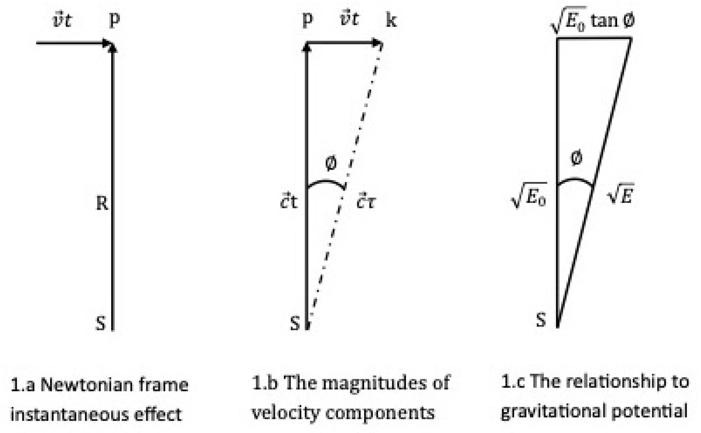
Figure 2.
The perihelion precession of Mercury.
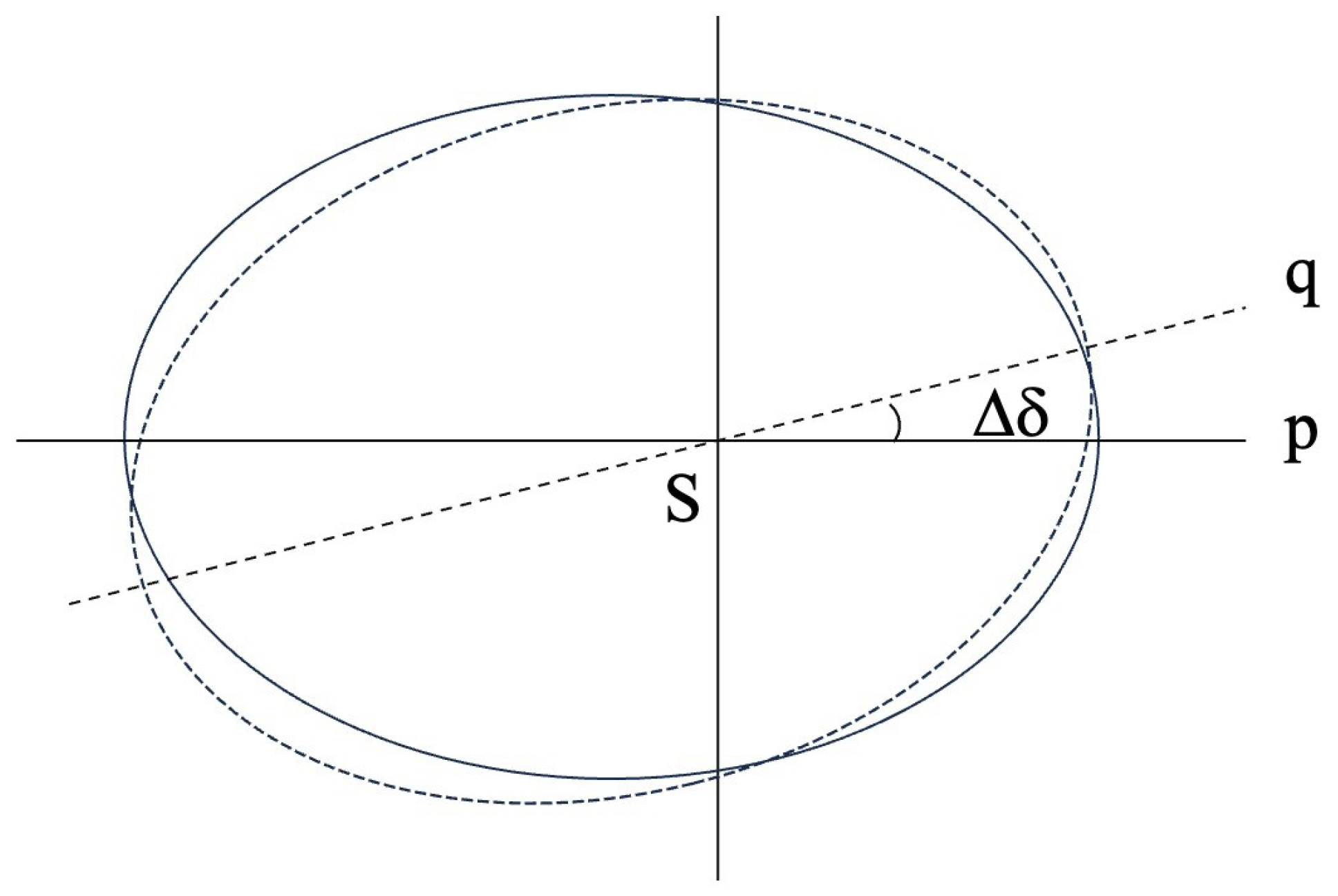
Figure 3.
Deflection of light by the Sun.
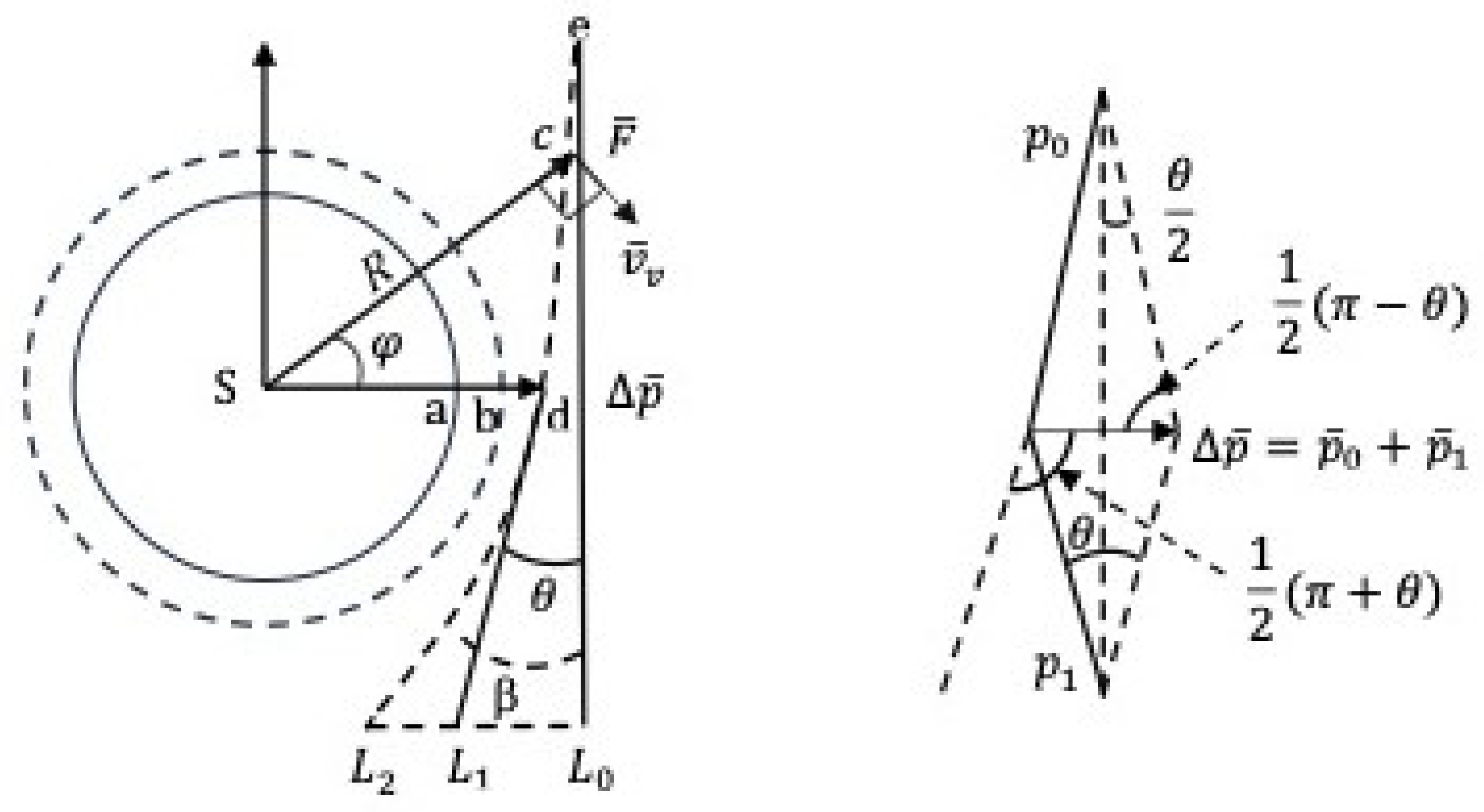
Figure 4.
Radar echo delay.
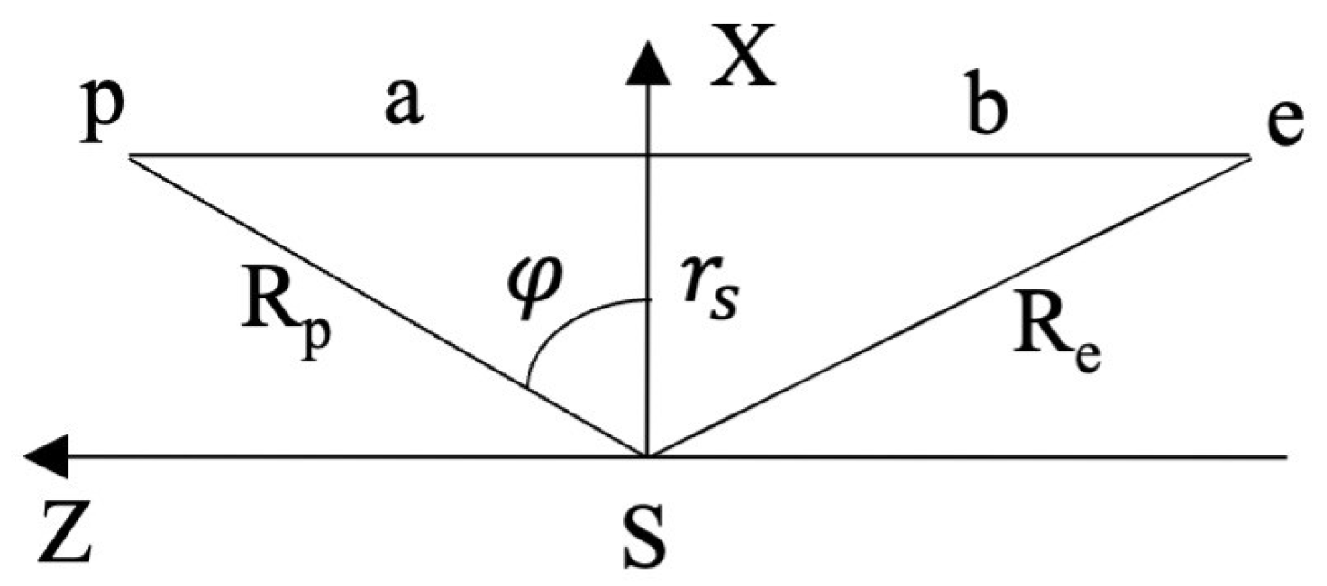
Figure 5.
The pyramid space for the velocitation effect of moving sources superposition.

Figure 6.
Milky May rotation curves.


Table 1.
Rotation velocity of Milky Way.
| kpc(to GC) | 8 | 10 | 15 | 20 | 25 |
| (km/s) | 201 | 179 | 147 | 127 | 114 |
| (km/s) | 0.271 | 0.191 | 0.106 | 0.068 | 0.049 |
| 48.58 | 84.63 | 234.57 | 480.35 | 842.16 | |
| 0.003 | 0.003 | 0.003 | 0.0025 | 0.002 | |
| 14.57 | 25.39 | 70.37 | 120.09 | 168.43 | |
| (km/s) | 240 | 228 | 222 | 209 | 197 |
| 235 | 231 | 220 | 208 | 199 | |
| 229 | 226 | 217 | 201 | 198 |
Disclaimer/Publisher’s Note: The statements, opinions and data contained in all publications are solely those of the individual author(s) and contributor(s) and not of MDPI and/or the editor(s). MDPI and/or the editor(s) disclaim responsibility for any injury to people or property resulting from any ideas, methods, instructions or products referred to in the content. |
© 2025 by the author. Licensee MDPI, Basel, Switzerland. This article is an open access article distributed under the terms and conditions of the Creative Commons Attribution (CC BY) license (http://creativecommons.org/licenses/by/4.0/).
Copyright: This open access article is published under a Creative Commons CC BY 4.0 license, which permit the free download, distribution, and reuse, provided that the author and preprint are cited in any reuse.


