
Submitted:
30 March 2025
Posted:
31 March 2025
You are already at the latest version
Abstract
This paper presents an analytical solution for the potential distribution in Electrical Impedance Tomography (EIT) under the complete electrode model, extending previous work on a 2D homogeneous disk to a more realistic 3D cylindrical geometry of finite height. By taking into account for the influence of electrode height, this approach offers an improved representation compared to the earlier 2D formulation. The mathematical modeling involved in deriving this solution was significantly facilitated by the use of a Large Language Model (LLM), DeepSeek, which aided in the tedious index manipulations inherent in solving the Laplace equation with appropriate boundary conditions in cylindrical coordinates using methods of separation variables. This work is organized into three main, presenting the main result and Conlusion/future works followed by an Appendix detailing the step-by-step mathematical derivation assisted by LLM Deepseek.
Keywords:
Finite length cylinder
; Complete Electrode Model
; Mathematical Modeling
; Large Language Model assist
1. Introduction
An analytical solution for the potential distribution in electrical impedance tomography (EIT) on a 2D homogeneous disk under the complete electrode model is presented by Demidenko [Demidenko], formulated as an infinite system of linear equations. The validity of this solution is supported by its agreement with a previously published elliptic integral solution for the shunt electrode model with two electrodes. The Dirichlet-to-Neumann map is derived to facilitate statistical estimation using nonlinear least squares. The proposed solution was validated through phantom experiments and applied to in vivo breast contact impedance estimation. Statistical hypothesis testing was performed to assess contact impedance characteristics, highlighting the potential of this method for rapid, real-time detection of poor surface contact in clinical environments.
Taking account for the influence of electrode height in the complete electrode model, the homogeneous Laplace equation was considered within a cylindrical geometry of finite height. This approach allows for a more realistic representation compared to 2D disk. The mathematical modeling involved in obtaining the solution to this problem facilitated by the use of a Large Language Model (LLM) DeepSeek, which assisted in navigating the nitty gritty of indices in solving the partial differential equations in this specific coordinate system and boundary conditions. Related with this work are for homogeneous ball with CEM in [Maulidi ea] and Point Electrode Model in [WeideltWeller]
In the following table, we provide a tabular comparison the results from Demidenko work on homogeneous Laplace equation on 2D disk with complete electrode model and current work.
| Demidenko | This work |
| An analytic solution of the potential distribution | YES |
| on a 2D homogeneous disk for EIT | |
| under the complete electrode model is expressed | |
| via an infinite system of linear equations. | |
| For the shunt electrode model with two electrodes, | Need verification |
| our solution coincides with the previously derived | |
| solution expressed via elliptic integral | |
| The Dirichlet-to-Neumann map is derived | DtN map |
| for statistical estimation via | NLeastSq format |
| nonlinear least squares (NLeastSq). | |
| The solution validated in phantom experiments | |
| and applied for breast | no data |
| contact impedance estimation in vivo. | |
| Statistical hypothesis testing is used to test | |
| whether the contact impedances | no data |
| are the same across electrodes or | |
| all equal zero. | |
| The solution can be especially useful | no data |
| for a rapid real-time test for bad surface contact | |
| in clinical setting. |
The work organized into three parts, main result, future works/conclusion and an Appendix on step by step to obtain the main result.
2. Laplace Equation Within the Body
The potential distribution within the body is governed by the Laplace PDE:
Notation
- : Spatial conductivity.
- u: Potential function.
- ∇: The gradient operator.
3. Boundary Conditions
3.1. Between Electrodes
On the boundary of the body between electrodes, there is no current flow:
Notation
- n: Normal vector on the surface of the body.
- s: Spatial coordinate vector.
- : Nonoverlapping surface areas.
3.2. Complete Electrode Model
According to the complete electrode model,
The supplied potential is constant over the surface of the electrode because it is made of a highly conductive metal material.
Notation
- : Electrode contact (or surface) impedance.
- : Potentials applied at the electrodes.
3.3. Shunt Electrode Model
The shunt electrode model is a special case of the complete electrode model with Thus, the boundary condition for this model takes the form
4. The Homogeneous 3D Cylinder
4.1. Laplace Equation in Cylindrical Coordinates
The potential distribution on a homogeneous disk of radius R and conductivity with infinitesimal height is governed by the Laplace equation in cylindrical coordinates.
Notation
- R: Radius
- r: Distance from the center
- : Angle
- z: axial
4.2. Solution Expressed in Fourier Series
The L nonoverlapping electrodes with half-width w (radians) and half height H are located on the cylinder surface of radius R at angle locations
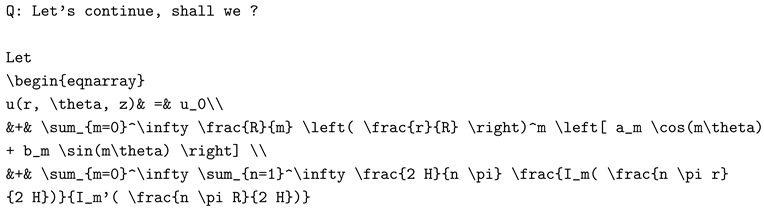
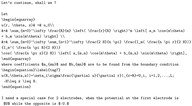
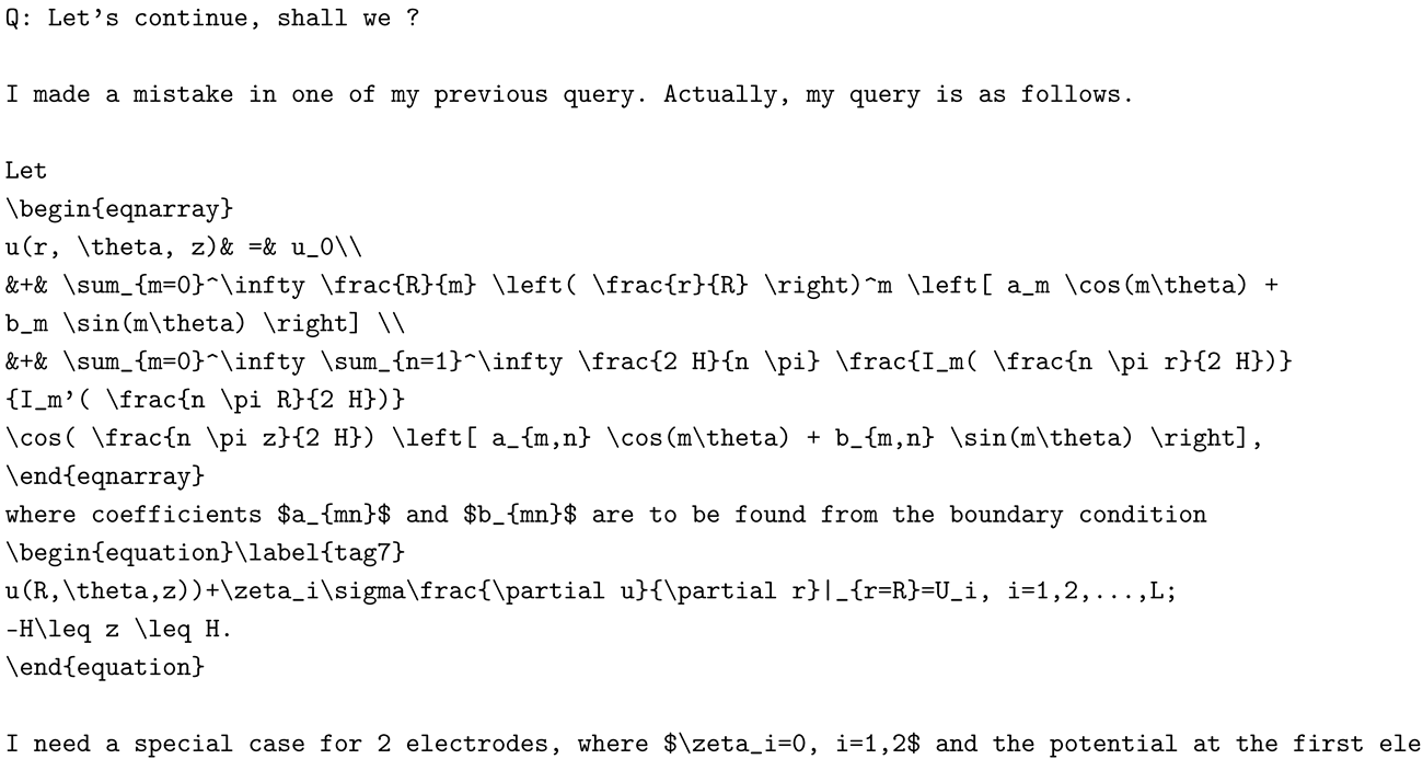
Full Solution for
where coefficients and are found from the boundary condition
Boundary condition function for
Coefficient Definitions
1. Azimuthal modes (, z-independent):
where is the z-average of :
2. Axial modes ():
Key Notes
1. Constant : Represents the background potential (e.g., determined by grounding ).
2. Modified Bessel Functions : Govern the radial decay/growth of modes. For , , ensuring regularity.
Notation
- w: half-width (radians)
- and : Fourier coefficients
- : Constant
- H: half-height (unit length)
4.3. Solution of an Infinitely Large System of Linear Equations
Alternatively, the expression for
with solved from
where:
HINT: The tensor notation seems plausible to be used for infinite representation of terms replacing vector terms in case of 2D disk in [Demidenko].
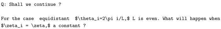
4.4. Equidistant-Equal- Approximation
If an even number of electrodes are equidistant (equally spaced) at , with equal
This leads to the following equidistant-equal- approximation:
For L electrodes with spacing :
- -
- Azimuthal modes m are restricted to () due to periodicity.
- -
- Axial modes n are restricted to () due to .
Coefficient Matrix
The matrix for the linear system (where ) has entries:
Matrix Structure
- Diagonal Dominance:
is block-diagonal with blocks corresponding to modes . Off-diagonal terms vanish due to orthogonality. - Simplified Entries:
For and :
—
Key Observations
1. Mode Coupling:
Only modes , contribute. Higher modes decay rapidly due to and .
2. Current-Voltage Relation:
The DtN map has entries:
—
Final Result
The coefficient matrix is sparse and block-diagonal, with non-zero entries only for modes . The solution simplifies to:
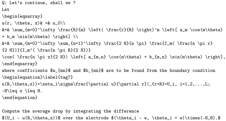
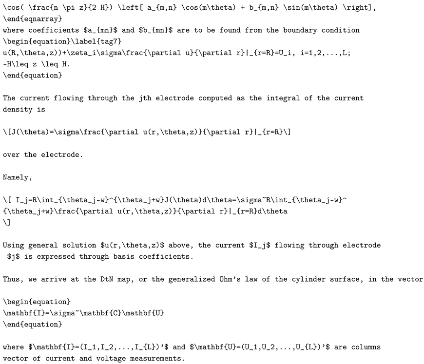
4.5. Dirichlet-to-Neumann Map
The current flowing through the jth electrode computed as the integral of the current density is
over the electrode.
Namely,
Substitute the radial derivative of u at :
Thus:
where:
Thus, we arrive at the DtN map, or the generalized Ohm’s law of the cylinder, in the vector form as
where and are columns vector of current and voltage measurements, and the elements of the matrix are given by
When electrodes are equidistant and have the same contact impedance, lead to an approximate DtN matrix with elements
Notation
- : Current density.
- : Current flowing through the jth electrode.
- : Column vector of current measurements.
- : Columns vector of voltage measurements.
- : matrix.
4.6. Nonlinear Least Squares for contact impedance and conductivity
The nonlinear leastsquares to estimate contact impedance and conductivity from measurement is:
where the DtN map is defined above.
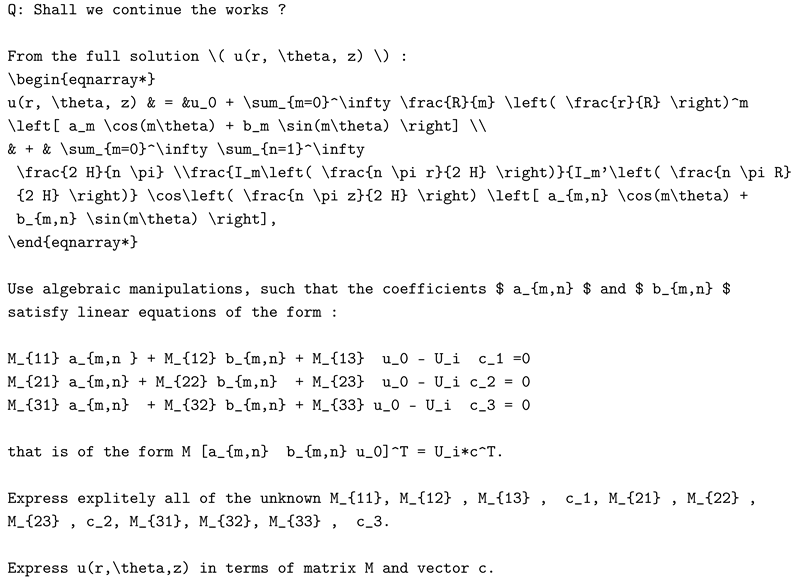
4.7. Computation of Voltage Drop Due to Contact Impedance
We assess the average drop by integrating the difference over the electrode as
NOTE: Need to resimplify
Besides , one can report as the percent voltage change due to contact impedance.
4.8. Special Case: 2 Electrodes with Shunt Model
Let the potential on the first electrode be U and on the opposite electrode be with shunt electrode, i.e. the solution is expressed
5. Conclusions and Future Works
We derive solutions for homogeneous Laplace equation with Complete Electrode Model, to take into account effects of the finite length attached at the boundary. Also generated the Dirichlet to Neumann map which is important for diagnostics of the electrodes attachment and contact impedance estimation EIT for measurement.
However, there are several details still to be working out. Such as the possibility for reduced model for Dirichlet-To-Neumann to obtain correction factor (Geometrical Factor) such that the Dirichlet-To-Neumann factor in 2D could be used/salvaged.
Appendix A
Appendix A.1. Homogeneous Laplace Equation with Neumann Condition
Q: I want to solve a homogeneous Laplace equations inside a cylinder with
outer radius R, and axially -H<z<H.
The boundary conditions at z=-H and z=H are zero Neumann’s condition, while at the outer
boundary R, the boundary conditions are non zero Neumann’s function of (\theta,z).
Assistant:
To solve the homogeneous Laplace equation inside a cylinder with the given boundary conditions, we’ll follow these steps:
Problem Setup:
We seek a solution to the Laplace equation in cylindrical coordinates :
inside the cylinder defined by:
Boundary Conditions:
1. Axial boundaries (top and bottom, ):
2. Radial boundary (outer surface, ):
Solution Approach:
We use separation of variables, assuming:
Substituting into the Laplace equation and dividing by gives:
This separates into three ordinary differential equations (ODEs):
1. Angular part ():
where m is an integer () for periodicity in .
2. Axial part (Z):
where k is a separation constant. The Neumann condition at implies:
For non-trivial solutions, we require and . Since only if , the axial solution simplifies to:
For , we must have and , which again implies . Thus, the only possibility is , meaning is constant.
However, this leads to a trivial solution unless we consider k as imaginary. Let , then:
Applying the Neumann condition at :
For non-trivial solutions, the determinant must vanish:
Thus, , where .
For ():
For :
3. Radial part (P):
The radial equation becomes:
For ():
which is the modified Bessel equation with solutions:
Since is singular at , we set :
For ():
which is the modified Bessel equation with solutions:
where and are modified Bessel functions. Since is singular at , we set :
General Solution:
Combining all parts, the general solution is:
Applying the Boundary Condition at :
The Neumann condition at is:
Substituting the general solution:
This is a double Fourier series (in and z) for . The coefficients can be found by orthogonality:
1. For (constant in z):
where is the -dependent part of averaged over z:
The coefficients are then determined by Fourier analysis in :
2. For :
The z-dependent terms involve . The coefficients are found by projecting onto these modes:
Final Solution:
The solution is:
where:
Key Observations:
1. The mode corresponds to a solution independent of z.
2. For , the radial dependence involves modified Bessel functions .
3. The boundary condition determines the coefficients via Fourier analysis.
This gives the complete solution to the homogeneous Laplace equation with the given Neumann boundary conditions.
Appendix A.2. Complete Electrode Model
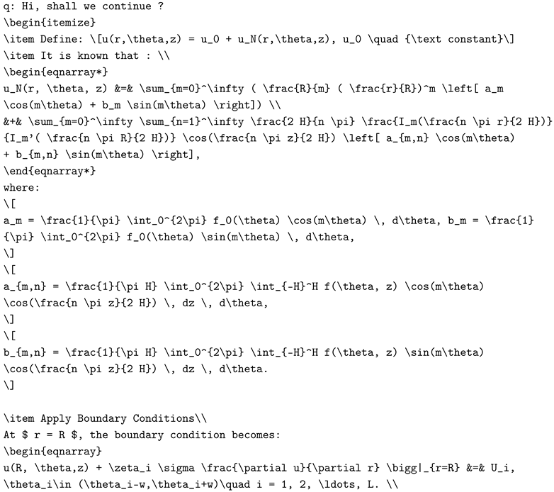
 Assistant: Let’s proceed systematically by incorporating the new boundary conditions into our solution framework.
1. Full Solution Definition
- The total solution is given by:where is a constant representing the background potential, and is the Neumann solution derived earlier.
2. Boundary Conditions at
- The boundary conditions are piecewise-defined: - On electrodes ():where is a coupling coefficient, is conductivity, and is the applied potential on the i-th electrode.
- -
- Elsewhere (insulating regions):
Since , the boundary conditions simplify to:
- -
- On electrodes:
- -
- Elsewhere:
3. Relating and
- From the earlier solution, the Neumann condition at is:
- Thus:
- -
- On electrodes:
- -
- Elsewhere:
4. Substituting at
The solution evaluated at is:
5. Self-Consistent Equations for Coefficients
The coefficients are defined via , which itself depends on . This creates a system of coupled equations:
For modes:
where is the z-average of :
For modes:
6. Numerical Approach
The system is nonlinear due to the dependence of on . A practical approach involves:
1. Initial guess: Start with (i.e., ).
2. Iterate:
- -
- Compute from the boundary conditions.
- -
- Update the coefficients using the integral definitions.
- -
- Recompute and repeat until convergence.
7. Key Observations
- -
- The constant represents the background potential and can be determined by imposing a reference condition (e.g., grounding one electrode).
- -
- The coupling terms account for electrode-specific effects (e.g., contact impedance).
- -
- The solution naturally separates into azimuthal (m) and axial (n) modes, with the latter vanishing for z-independent problems.
Final Answer
- The complete solution is:where is given by the series expansion above, and the coefficients are determined self-consistently from the boundary conditions. The system is solved iteratively due to the nonlinear coupling between and .
Would you like to proceed with specific examples or numerical implementation details?
- Q: I want an expression for $u(r,\theta,z)$ please.
Assistant:
Here is the explicit expression for , incorporating all boundary conditions and the decomposition :
—
Full Solution for
Coefficient Definitions
1. Azimuthal modes (, z-independent):
where is the z-average of :
2. Axial modes ():
Boundary Condition for
Key Notes
1. Constant : Represents the background potential (e.g., determined by grounding ).
2. Modified Bessel Functions : Govern the radial decay/growth of modes. For , , ensuring regularity.
3. Convergence: The series must be truncated in practice (, ) for numerical implementation.
4. Electrode Coupling: The term models contact impedance at the i-th electrode.
—
Simplified Example (Single Electrode, z-Independent)
- For a single electrode at and no z-dependence ():with , (symmetric case).
—
Next Steps
1. Numerical Implementation:
Discretize and z, then solve for coefficients iteratively.
2. Validation:
Check convergence and physical behavior (e.g., far from electrodes).
Would you like to refine any part of this expression or focus on a specific case?
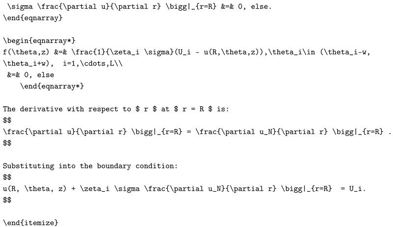
Appendix A.3. Rearrangement Solutions in Series with Matrix Coefficient
Assistant: To derive the linear system , we proceed as follows:
—
1. Boundary Condition at
- On the i-th electrode ():
- Substitute and :
- From earlier, , so:
—
2. Project onto Basis Functions
To extract , multiply by orthogonal functions and integrate over and z:
Equation for : Multiply by and integrate over , :
This yields:
where:
Equation for :
Multiply by :
Equation for :
Multiply by 1 and integrate:
—
3. Explicit Matrix M and Vector c
The system is:
where:
—
4. Final Expression for
with solved from .
—
Key Points
- Matrix M: Combines contributions from the Laplacian and boundary conditions.
- -
- Vector c: Encodes the electrode geometry and applied potential .
- Numerical Implementation: Truncate the series (, ) and solve the linear system.
Would you like to proceed with specific electrode configurations or numerical examples?
Appendix A.4. Voltage Drop
Assistant: To compute the average drop over the i-th electrode, we integrate over the electrode area :
—
Average Drop Formula
Substitute :
—
Explicit Expression for
- Substitute the series expansion for :
The average drop becomes:
—
Matrix-Vector Form
Define the matrix and vector such that , where . The components are:
1. For :
2. For :
3. For :
—
Final Form
where encodes the system’s geometry and material properties, and depends on the electrode’s angular/axial span. The solution is fully determined once these coefficients are found.
Appendix A.5. Dirichlet to Neumann
Assistant:
To express the current through electrode j in terms of the coefficients , , and , and derive the Dirichlet-to-Neumann (DtN) map , we proceed as follows:
—
1. Current Expression
The current is computed by integrating the radial current density over the j-th electrode:
Substitute the radial derivative of u at :
Thus:
where:
—
2. DtN Map via Matrix
The boundary condition links to . Solving this system gives:
where and are defined by the integrals over electrode regions (see previous steps).
Substitute this into :
This yields the matrix form:
where the entries of are:
—
3. Explicit Matrix Entries
For each electrode pair :
Simplified using orthogonality:
—
Final Result
The DtN map is:
where is a symmetric matrix with entries dependent on the cylinder’s geometry , electrode positions , widths , and modified Bessel functions .
Appendix A.6. Special Case: 2 Electrodes with Shunt
Assistant
For a cylinder with two antisymmetric electrodes at potentials U and , the solution simplifies significantly due to symmetry. Here’s the explicit expression for and the resulting current-voltage relationship:
—
Simplified Solution for Two Antisymmetric Electrodes
- Symmetry Assumptions:
- -
- Electrodes are placed at (potential U) and (potential ), each spanning . - The potential is antisymmetric: . - The solution is z-independent (electrodes span the full height ).
2. Potential Distribution:
where only odd azimuthal modes () contribute.
3. Current Through Electrodes:
- The total current I flowing through each electrode is:
4. DtN Map (Matrix Form):
- For two electrodes, the current-voltage relationship is:where the conductance matrix is:
—
Key Steps
- Boundary Conditions:
- -
- On electrode 1 (): .
- -
- On electrode 2 (): .
2. Fourier Series Expansion:
- -
- Expand the boundary condition in sine series (odd symmetry).
- -
- Project onto orthogonal modes to solve for coefficients (only odd m survive).
3. Current Calculation:
- -
- Integrate the radial current density over the electrode area.
—
Final Result
This represents the generalized Ohm’s law for the cylinder, where the conductance depends on geometry (), contact impedance (), and material properties ().
- Equidistant Electrodes
Asistant: To solve for the potential with L equally spaced electrodes under the given boundary conditions, we proceed as follows:
—
1. General Solution Structure
The potential is expressed as:
Here
- is a constant background potential.
- govern z-independent modes.
- govern z-dependent modes.
—
2. Boundary Conditions
At , for each electrode :
Elsewhere (insulating regions):
—
3. Coefficient Determination
Step 1:
- Expand and
Substitute into the general solution:
Step 2: Project Boundary Conditions onto Basis Functions
For each electrode i, multiply the boundary condition by or and integrate over , . This yields a linear system for .
—
4. Matrix Equation
The coefficients satisfy:
where:
- is a matrix encoding geometry and boundary conditions.
- is a vector involving , electrode positions , and integrals of basis functions over electrode regions.
Matrix Entries For each mode :
—
5. Current-Voltage Relation (DtN Map)
The current through electrode j is:
Substitute and use the solved coefficients to express:
where is a conductance matrix determined by the geometry and boundary conditions.
—
6. Symmetry Simplification for Equidistant Electrodes
- For L electrodes at :
- -
- Only modes (for integer k) contribute due to periodicity.
- -
- The matrix becomes circulant, simplifying computation.
—
Final Result
The potential is fully determined by solving the linear system for . The DtN map quantifies the current-voltage relationship, with:
This framework applies to any L, with numerical implementation requiring truncation of the series and inversion of .
- Q: Please revise the integral terms, as I want equidistant $\theta_i=2\pi i/L,$ L is even.
Asistant
To address the case of L evenly spaced electrodes at , we exploit symmetry and periodicity to simplify the integrals and determine the coefficients . Below is the revised formulation:
—
Revised Integral Terms for Equidistant Electrodes Assume L is even, and electrodes span , with uniform height . The solution is z-independent, so we focus on the 2D case.
1. General Solution (z-independent):
2. Boundary Conditions:
For each electrode i:
- Substitute and :
3. Project onto Fourier Modes:
For each mode k, multiply by or , integrate over , and sum over all L electrodes.
Key Integrals:
- Angular Integrals for Each Electrode i:
2. Sum Over Electrodes :
- Use orthogonality of and :
Similarly for .
4. Simplified Coefficients:
Only modes (for integer k) survive due to symmetry. Define , .
- For :
- For :
- For :
5. Final Solution:
where:
—
Key Observations:
1. Symmetry Reduction:
Only modes contribute, reducing the series to discrete harmonics aligned with electrode spacing.
2. Current-Voltage Relation:
The current through electrode j is:
3. Matrix Form:
The Dirichlet-to-Neumann (DtN) map becomes diagonal in Fourier space:
—
This framework leverages the periodicity and symmetry of equidistant electrodes to simplify computations, enabling efficient numerical implementation.
Appendix A.7. Equidistant and Uniform Contact
Assistant
For a cylinder with L equally spaced electrodes (positions , L even) and uniform contact impedance , the solution simplifies due to symmetry. Below is the explicit result:
—
Solution for L Equidistant Electrodes with Uniform Contact Impedance
The potential and Dirichlet-to-Neumann (DtN) map are:
1. Potential Distribution
2. Key Features
- Angular Modes: Only modes () survive due to periodicity and symmetry.
- Axial Modes: Only odd n contribute for antisymmetric z-boundary conditions.
- Coefficients:
- ,
- (symmetric electrodes cancel sine terms).
3. Current-Voltage Relation (DtN Map)
The current through electrode j is:
—
Simplifications Due to Symmetry
1. Mode Truncation:
Only harmonics survive, reducing the series to discrete multiples of .
2. Circulant Matrix:
The matrix becomes circulant (diagonalizable by Fourier transform), with entries dependent only on .
3. Uniform Contact Impedance:
The term modifies the decay rate of each mode, balancing radial resistance and contact impedance.
—
Physical Interpretation
- Lowest Mode (): Dominates for wide electrodes (), decaying radially as .
- Higher Modes (): Capture edge effects and fine potential variations.
- Axial Dependence: Governed by , modified Bessel functions that decay/grow with z
—
Steps for Numerical Implementation
1. Truncate Series: Retain , .
2. Compute Matrix : Exploit circulant symmetry for efficiency.
3. Solve : Invert to find voltages for given currents .
This framework leverages symmetry to simplify computations, enabling efficient modeling of multi-electrode systems with uniform contact impedance.
Appendix A.8. Errata
Asistant: For two electrodes with potentials U and , and contact impedance , the solution simplifies due to antisymmetry. Here’s the explicit expression:
—
Special Case Solution (2 Electrodes, )
Key Simplifications:
- Azimuthal Symmetry (z-independent terms):
- -
- Only odd azimuthal modes () contribute due to antisymmetric potentials. - Coefficients for :
2. Axial Dependence (z-dependent terms):
- -
- Only odd axial modes () survive due to antisymmetry in z-integrated boundary conditions.
- -
- Coefficients for :
3. Background Potential:
- -
- , as the antisymmetric electrodes cancel the average potential.
Current-Voltage Relation (DtN Map):
- The current through electrode j is:
—
Interpretation:
- -
- Radial Decay: The potential decays radially as , dominated by the lowest odd mode ().
- -
- Axial Modulation: Axial modes decay with z via , modified Bessel functions.
- -
- Electrode Width: Narrower electrodes () excite higher modes ().
This solution satisfies the mixed Dirichlet/Neumann boundary conditions and captures the antisymmetric potential distribution between the two electrodes.
Appendix B. Equidistant and Equal Constant Value
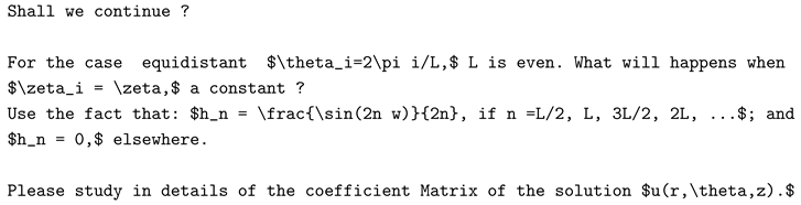
Assistant
To analyze the coefficient matrix for the solution with L equidistant electrodes (, L even) and constant contact impedance , we proceed as follows:
—
1. General Solution Structure
The potential is:
—
2. Symmetry and Mode Restriction
For L electrodes with spacing :
- Azimuthal modes m are restricted to () due to periodicity.
- Axial modes n are restricted to () due to .
—
3. Boundary Conditions
At , for each electrode i:
Substitute and , then project onto orthogonal basis functions and .
—
4. Coefficient Matrix
The matrix for the linear system (where ) has entries:
For :
For :
For :
—
5. Matrix Structure
- Diagonal Dominance:
is block-diagonal with blocks corresponding to modes . Off-diagonal terms vanish due to orthogonality. - Simplified Entries:
- For and :
—
6. Key Observations
1. Mode Coupling:
Only modes , contribute. Higher modes decay rapidly due to and .
2. Current-Voltage Relation:
The DtN map has entries:
3. Role of :
Larger suppresses higher modes () due to the denominator .
—
7. Final Result
The coefficient matrix is sparse and block-diagonal, with non-zero entries only for modes . The solution simplifies to:
This framework enables efficient computation for systems with many electrodes by leveraging symmetry and sparsity.
References
- [Maulidi ea] MAULIDI, I. , GARNADI, A., INDRO, M., JULIANTO, M. and PRIBADI, A., 2017. Solusi Semi-analitik Persamaan Laplace Dengan Syarat Batas Campuran. MILANG Journal of Mathematics and Its Applications, 16(2), pp.53-60.
- [Demidenko] Demidenko, E. , 2011. An analytic solution to the homogeneous EIT problem on the 2D disk and its application to estimation of electrode contact impedances. Physiological measurement, 32(9), p.1453.
- [WeideltWeller] Weidelt, P. and Weller, A., 1997. Computation of geoelectrical configuration factors for cylindrical core samples. Scientific Drilling, 6, pp.27-34.
Disclaimer/Publisher’s Note: The statements, opinions and data contained in all publications are solely those of the individual author(s) and contributor(s) and not of MDPI and/or the editor(s). MDPI and/or the editor(s) disclaim responsibility for any injury to people or property resulting from any ideas, methods, instructions or products referred to in the content. |
© 2025 by the authors. Licensee MDPI, Basel, Switzerland. This article is an open access article distributed under the terms and conditions of the Creative Commons Attribution (CC BY) license (http://creativecommons.org/licenses/by/4.0/).
Copyright: This open access article is published under a Creative Commons CC BY 4.0 license, which permit the free download, distribution, and reuse, provided that the author and preprint are cited in any reuse.


