An exact (O(n^2)) solution to the Travelling Salesman Problem

1. Introduction

The TSP was first formulated in 1930 and asks the following question: “Given a list of cities and the distances between each pair of cities, what is the shortest possible route that visits each city exactly once and returns to the original city?” [1].

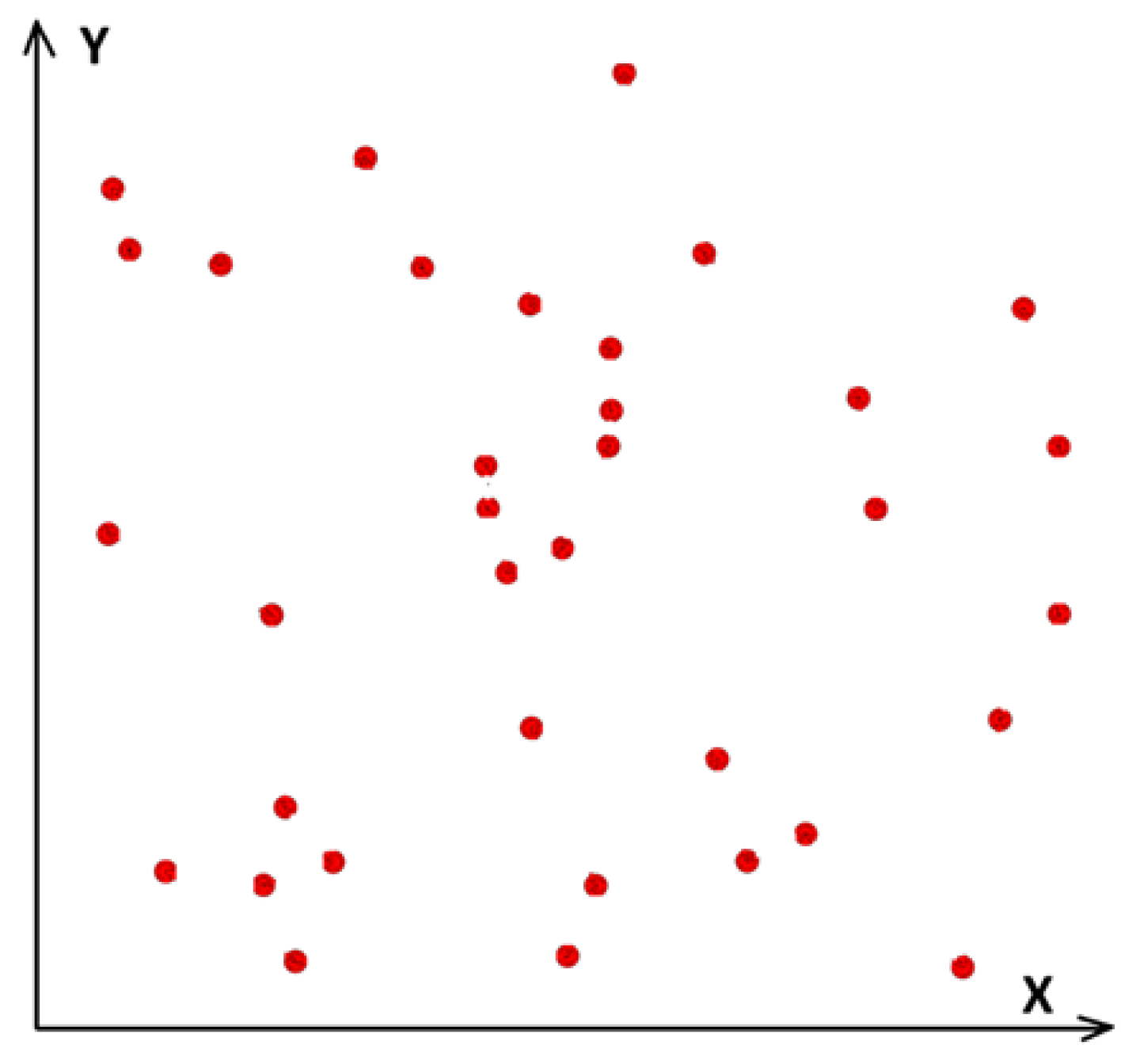
Alternatively, we can be presented with a cloud of points (cities) on a plane where each point is defined by its X and Y coordinate and our goal is to find the shortest graph connecting all the points once and returning to the original point. In this case each distance between 2 points k and j can be found by using the Pythagorean formula: ${(Xk-Xj)}^2+{(Yk-Yj)}^2={Distance}^2$, where (Xk , Yk) and (Xj, Yj) are the points k and j

Figure 1. An example of a cloud of points (cities) on a plane where each point is defined by its X and Y coordinate.

Figure 1. An example of a cloud of points (cities) on a plane where each point is defined by its X and Y coordinate.

The TSP has implications in many areas such as logistics and others [2].

Although, the TSP has been considered an NP-hard problem, and no known polynomial-time solution to solve it exactly [3] has been proposed yet, this algorithm proposes an exact (O(n^2)) polynomial-time solution.

This method will focus on iteratively solving the problem for n cities first and then for an n+1 city next. Then repeating the process for an n+2, n+3 and etc. until all our cities will be joined by the shortest possible route.

This algorithm is similar to many others Convex Hull Insertion Methods including methods like this one [4] or that one [6]. But unlike others it starts not from outside the cloud but from inside it. This approach agrees with the fact that the shortest path must not intersect itself and lie on the convex hull or within it. [5]

We will be adding our cities (points) starting from the cities closest to their “center of the cloud”. In other words, starting from the cities closest to their centroid or the point on the plane with the average X and average Y coordinates where Xcentroid = (X1 + X2 + … + Xn)/n , Ycentroid = (Y1 + Y2 + … + Yn)/n and (Xi, Yi), 1 <= i <= n are the coordinates of our points.

Figure 2. An example of a cloud of points (cities) on a plane and their centroid.

Figure 2. An example of a cloud of points (cities) on a plane and their centroid.

2. Definitions

But before we start describing the method itself let’s define a few things.

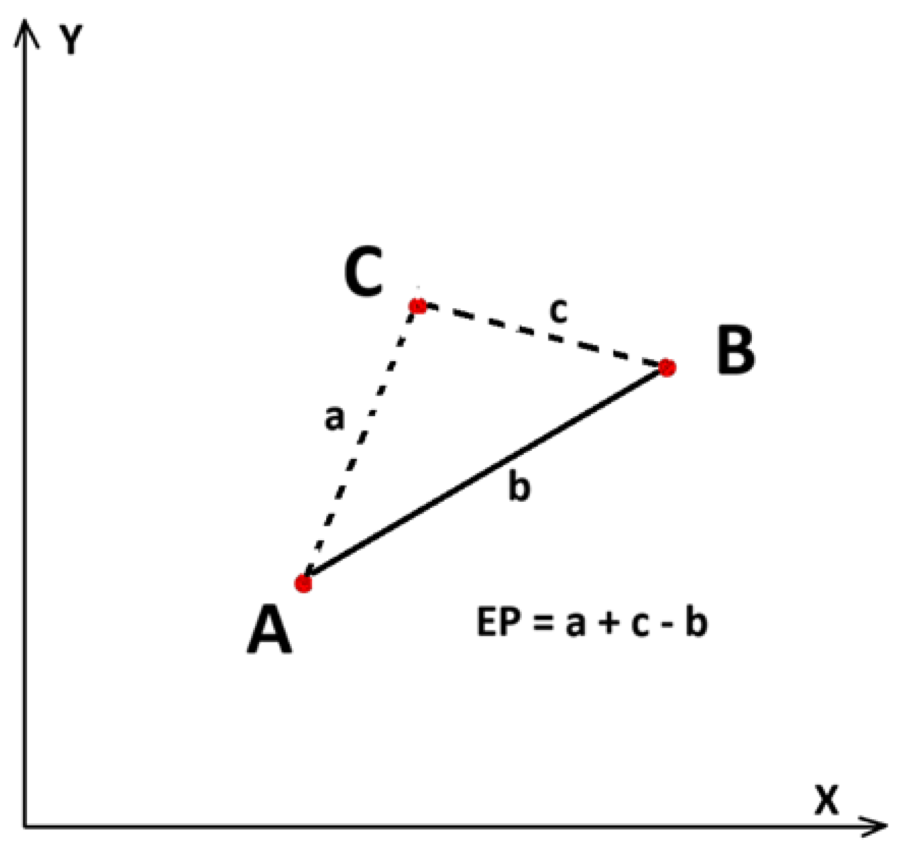
Let’s imagine 2 points A and B and connect them creating a path from point A to point B. Thus, we have got a line segment [AB]. Now, let’s add a third point C which is not on the line segment [AB]. Let’s now connect our point C to the other two points A and B. Once we joined the third point, we have got 2 possible paths we could travel from A to B. The first one is the direct path from A to B with the distance equal to amount of the line segment [AB]. The second path is through the point C and its distance is equal to [AC] + [CB]. Since the line segment [AB] is the shortest path from A to B then it is obvious that [AC] + [CB] > [AB].

Let’s now call [AC] + [CB] – [AB] an Excess Path (EP) we need to travel from A to B when we are not using the shortest and direct path. So, EP = [AC] + [CB] – [AB] or if we imagine a triangle we can then label our sides: [AB] as b, [AC] as a, and [CB] as c and thus EP = a + c – b

Figure 3. An example of calculating Excess Path.

Figure 3. An example of calculating Excess Path.

3. Lemma

Now, let’s define and prove a Lemma.

If we are given that we have already solved TSPmin for n points, and we are joining new n + 1, n + 2, etc. points and:

3.1. Each next n + 1, n + 2, etc. point we are joining will be farther and farther away from our global centroid for our full set of F points, where 1 <= n <= F

We calculate the EPi for each line segment (where 1 <= i <= n) of our TSPmin and take EPmin = MIN(EP1, EP2, …, EPn), then join our new n+1 point to the two endpoints of the newly found EPmin line segment thus creating the sides amin and cmin and also erasing the side bmin

Figure 4. An example depicting the location of the minimal Excess Path.

Figure 4. An example depicting the location of the minimal Excess Path.

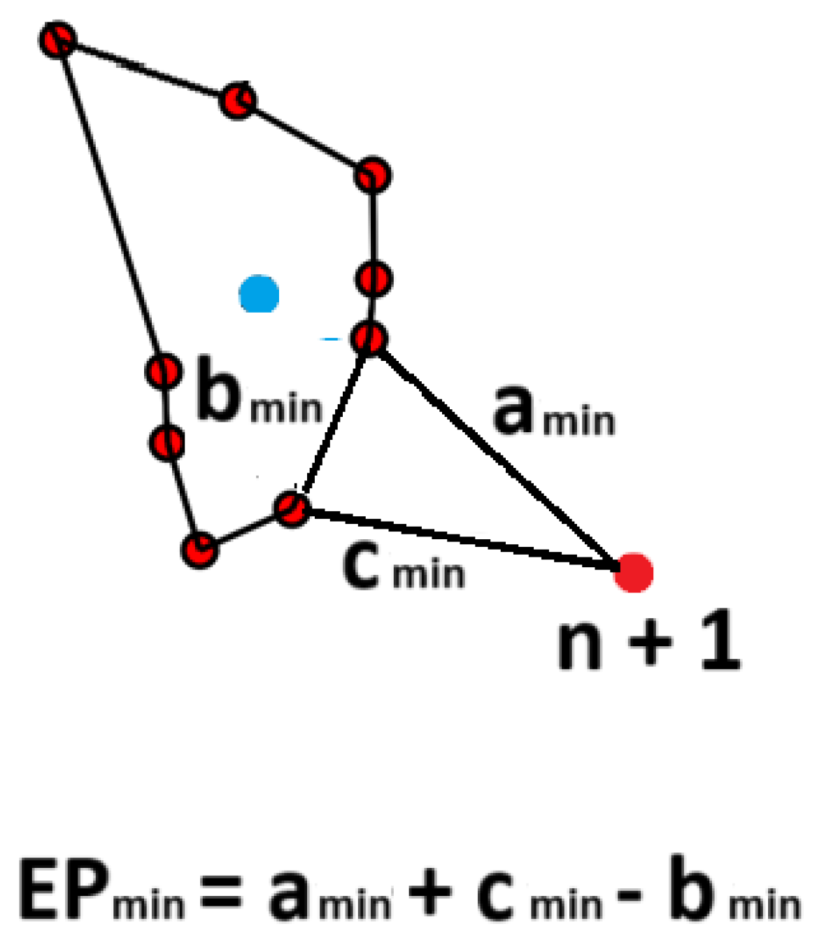
Then our newly created path TSPmin, n+1 = TSPmin + MIN(EP1, EP2, …, EPn) will also be a valid path and the shortest path for n + 1 points and joining each next point that satisfy the 3.1 criteria will also produce the shortest path for each next n + 2, n + 3, etc. point, where 1 <= n <= F

Figure 5. An example depicting a newly created shortest path for n + 1 points.

Figure 5. An example depicting a newly created shortest path for n + 1 points.

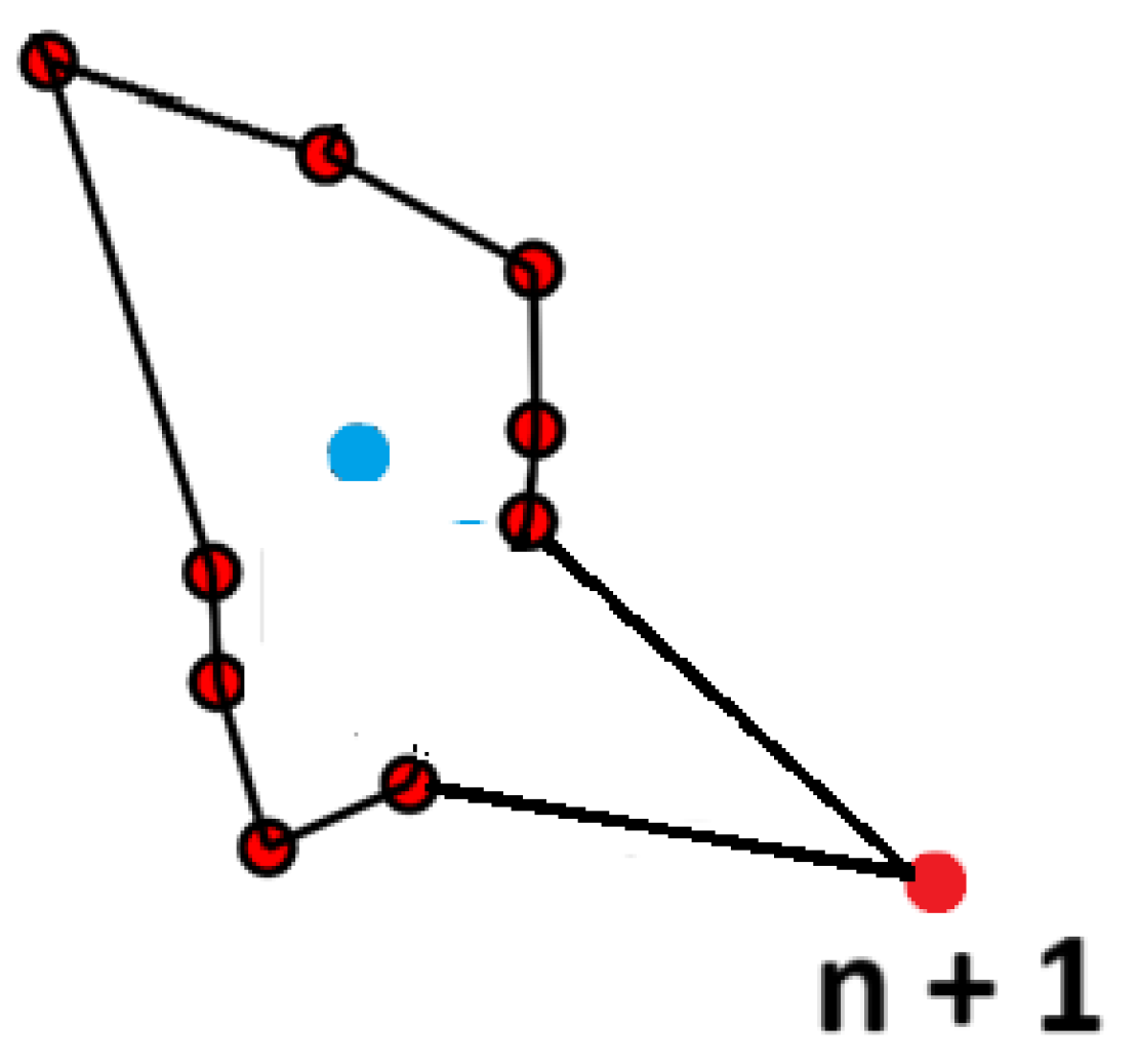
It will still be a path where you visit each point only once and return to the original point because we are not interrupting our path, we are only extending it by adding the excess route to our new point and erasing the “old direct” route.

And if we obey the 3.1 condition of our Lemma, we can guarantee that on every step of joining a new point the newly created convex hull will be “empty” inside and will not enclose any other points except those on its border. On the other hand, it was proven [5] that the shortest path will always lie on the convex hull or inside it. But in our case, there will be no points inside a border on each iteration. That leaves us with the only conclusion that the convex hull’s border on each iteration will itself be the shortest path.

Our new TSPmin, n+1 will still be the shortest path for n + 1 because TSPmin, n+1 = TSPmin + MIN(EP1, EP2, …, EPn). Again, we took the shortest route TSPmin and we added MIN(EP1, EP2, …, EPn) to it thus ensuring our new route will also be the shortest route.

Let’s assume the opposite and say that a different shortest route TSPmin, n+1, alt exists and it does not include our original route TSPmin. Then, by removing our n + 1 point, we would find out that for the same n points yet another shortest route TSPmin, alt exists and it is different from our original shortest route TSPmin. Which is a contradiction.

4. The Algorithm

Let’s now return to the method itself.

From our cloud of n points let’s take the closest to the centroid 3 points first and connect them. We have got a triangle and its perimeter is the shortest path TSPmin, 3 for the three connected points.

Now, let’s select the 4^th point closest to the centroid and then find out the line segment where EPi = MIN(EP1, EP2, EP3), 1 <= i <= 3 and connect our 4^th point to the line segment’s endpoints.

According to our Lemma the new path for the 4 points we just created is also the shortest path. Then we can repeat the same process for our 5^th, 6^th, and etc. point until all the points of our cloud are connected.

This step-by-step process is depicted below:

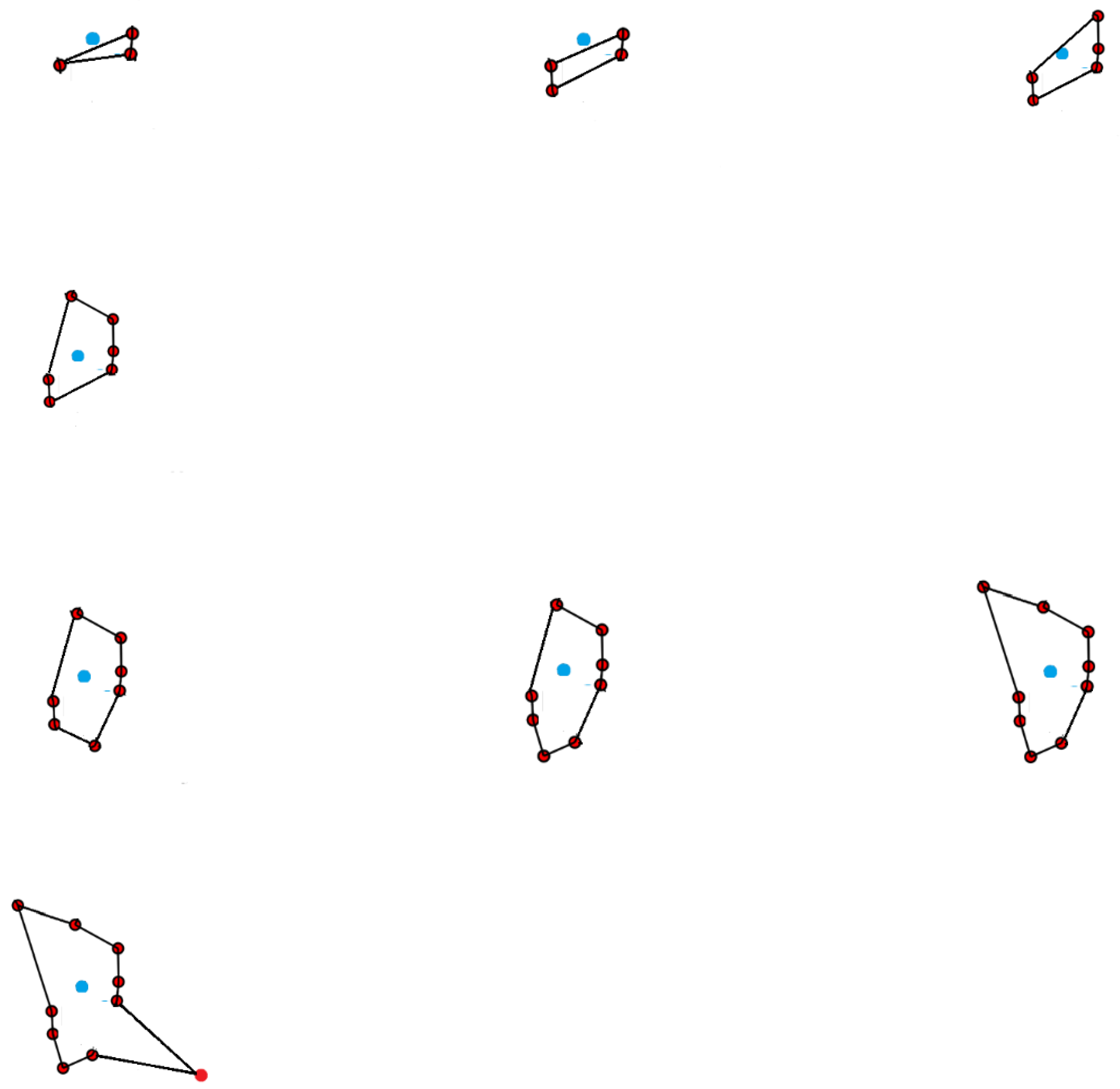
Figure 6. An example showing 8 iterations of the algorithm that expands the shortest path to the points more distanced from their centroid.

Figure 6. An example showing 8 iterations of the algorithm that expands the shortest path to the points more distanced from their centroid.

5. Special Cases

5.1. When the 3 or more points closest to the centroid lie on the same line segment, we treat these points as one line segment and build the first triangle on it and the next closest to the centroid 2 points.

5.2. When a point coincides with the centroid, we treat it as a vertex of our first triangle

5.3. When there are 2 or more points with the same distances from the centroid, we are joining them consecutively in no particular order

6. The Number of Computations Needed

The question arises how many calculations of EP in total using this method you would have to make in order to find the shortest possible route for n points? Remember that we have to find out the total number of each EPj,k = aj,k + cj,k – bj,k where 3 <= j <= n-3 and 1 <= k <= j. Each distance between the points (cities) aj,k , cj,k , bj,k has been given already in the beginning or pre-calculated using their x and y coordinates and the Pythagorean formula.

Let’s disregard the pre-calculations you will have to make to find each city’s distance from the centroid and arrange the cities accordingly. These distances from each point ($Xn,Yn$) can be easily found by using the formula:

$${(Xcentroid-Xn)}^2+{(Ycentroid-Yn)}^2={Distance}^2.$$

On the very first step, when we join our 4^th point, we calculated the EP three times.

On the next step joining the 5^th point, we calculated the EP four times and etc.

So, to estimate how many calculations of EP in total you would have to make we will have to calculate the sum of 3 + 4 + 5 + … + etc. and the sequence will follow the arithmetic progression where the number or terms will be equal to (n – 3), the common difference will be 1 and the first term will be 3.

The sum of arithmetic progression is described by the formula Sn = $n/2(2a+\left(n-1\right)d)$, where n is the number or terms, a is the first term and d is the common difference.

By substituting our numbers to the formula, we are getting Sn-3 = (n – 3) (n + 2) / 2. This formula represents a (O(n^2)) polynomial-time quadratic solution.

Let’s compare that (n – 3) (n + 2) / 2 number to the Brute-force search method that yields (n – 1)! / 2 number of calculations. If we take n = 10, then the Brute-force search would require 181,440 computations from us. With the same n = 10 this method will require only 42 computations. Moreover, the more is the number of cities n, the more efficient and quicker this method is going to be in comparison to the Brute-force search method.

7. Conclusions

In this article, a new exact (O(n^2)) quadratic-time iterative algorithm of solving TSP is proposed.

The algorithm solves the problem by building the shortest possible route to a small number of close to the centroid points first, and then iteratively expanding the route to all the points.

This article also estimates the number of computations needed to support this method and shows this method’s big advantage over the standard Brute-force search method.

References

- Eugene, L. Lawler, Jan Karel Lenstra, A. H. G. Rinnooy Kan, and David B. Shmoys. The Traveling Salesman Problem: A Guided Tour of Combinatorial Optimization. John Wiley & Sons, 1985.
- David, L. Applegate, Robert E. Bixby, Vasek Chvatal, and William J. Cook. The Traveling Salesman Problem: A Computational Study. Princeton University Press, 2007.
- Michael, R. Garey and David S. Johnson. Computers and Intractability: A Guide to the Theory of NP Completeness. W. H. Freeman, 1979.
- Zheng, M. TSP Algorithm based on Convex Hull Insertion Method. Preprints 2024, 2024061760. [Google Scholar] [CrossRef]
- Dan Kai. Solving the Traveling Salesman Problem Using Dynamic Programming Based on Optimal Insertion Subsets [D]. Nanchang University: 2020.
- Marko, D.; Milton, S. Apple Carving Algorithm to Approximate the Traveling Salesman Problem from Compact Triangulation of Planar Point Sets. Int. J. Adv. Comput. Sci. Appl. (IJACSA) 2020, 11. [Google Scholar]
Disclaimer/Publisher’s Note: The statements, opinions and data contained in all publications are solely those of the individual author(s) and contributor(s) and not of MDPI and/or the editor(s). MDPI and/or the editor(s) disclaim responsibility for any injury to people or property resulting from any ideas, methods, instructions or products referred to in the content. |
© 2025 by the authors. Licensee MDPI, Basel, Switzerland. This article is an open access article distributed under the terms and conditions of the Creative Commons Attribution (CC BY) license (http://creativecommons.org/licenses/by/4.0/).
Copyright: This open access article is published under a Creative Commons CC BY 4.0 license, which permit the free download, distribution, and reuse, provided that the author and preprint are cited in any reuse.