Submitted:
28 March 2025
Posted:
28 March 2025
You are already at the latest version
Abstract
The China–Mongolia arid region adjacent to the Altai Mountain (CMA) has a sensitive ecosystem that relies heavily on both terrestrial water (TWS) and groundwater storage (GWS). However, during the 2003–2016 period, the CMA experienced significant glacier retreat, lake shrinkage and grassland degradation. To illuminate the TWS and GWS dynamics in the CMA and the dominant driving factors, we employed high-resolution (0.1◦) GRACE (Gravity Recovery and Climate Experiment) data generated through random forest (RF) combined with residual correction. The downscaled data at a 0.1° resolution illustrate the spatial heterogeneity of TWS and GWS depletion. The highest TWS and GWS decline rates were both on the north slope of the Tianshan River Basin (NTRB) of the Junggar Basin of Northwestern China (JBNWC) (28.39 mm/yr and -32.17 mm/yr, respectively). Human impact played a primary role in TWS decreases in the JBNWC, with a relative contribution rate of 61.88% compared to the climatic contribution (38.12%). A notable shift—from climatic (2002-2010) to anthropogenic factors (2011-2020)—was observed as the primary driver of TWS decline in the Great Lakes Depression region of western Mongolia (GLDWM). To maintain ecological stability and promote sustainable regional development, effective action is urgently required to save essential TWS from further depletion.
Keywords:
terrestrial water storage
; drivers
; human interventions
; GRACE (FO) satellites
; climate change
1. Introduction
Terrestrial water storage (TWS), which includes water stored in rivers, lakes, reservoirs, soil, groundwater systems, snow, glaciers and vegetation, plays a crucial role in the global hydrological cycle and land–atmosphere interactions [1]. TWS is essential for determining hydrologic transport and water availability [2], serving as a key indicator of water resource vulnerability [3]. However, accurately monitoring the dynamic changes in TWS, particularly in data-scarce regions, remains challenging due to the limited availability of field observation gauges, the high costs associated with installing and maintaining instrument networks, lack of data digitization and sharing, and significant uncertainties in hydrological and land surface models [4,5]. The China–Mongolia arid region adjacent to Altai Mountain (CMA) is a typical Asian inland arid zone, representing a key area of the Silk Road. The Junggar Basin of Northwestern China (JBNWC) and the Great Lakes Depression region of western Mongolia (GLDWM), which are located in the southern and northern Altai Mountains, are highly sensitive to global climate change, and their ecological environment is fragile [6,7]. The JBNWC has experienced population growth and urban expansion, which have increased the need for irrigation[8], while the GLDWM is primarily used for livestock farming, with mineral extraction also expanding in the past two decades [9,10]. Therefore, TWS plays a critical role in determining water availability, ensuring water and ecological security, and maintaining ecosystem functions in the CMA. Under the combined influence of climate change and human activities, monitoring the TWS changes in the CMA is of great significance for addressing regional water resource management and sustainable development.
The Gravity Recovery and Climate Experiment (GRACE) satellites provide an effective means of detecting TWS changes over large-scale regions, particularly in areas with limited in situ data [11]. To date, GRACE has been widely used for various applications, including identifying TWS variations at regional and global scales [11,12], assessing groundwater depletion [13,14], monitoring droughts [15,16], and detecting land subsidence [17]. However, GRACE data have some limitations that hinder their application for long-term hydrological changes at local scales, such as data gaps [18] and coarse spatial resolution [19]. Notably, there is an ~1-year gap between the original GRACE mission (launched in 2002) and its follow-on (GRACE-FO) mission, launched in 2018, which affects the continuity of monitoring water storage changes [20]. Furthermore, caution is necessary when applying GRACE observations to regions with heterogeneous geomorphological features [21]. Specifically, the GRACE observation footprint is approximately 200,000 km² due to the orbit height (~450×450 km = ~200,000 km²), which is too coarse to meet the detailed needs of water resource managers [22]. As a result, improving the spatial resolution of GRACE data holds significant potential for broadening their application.
There are two commonly used methods for GRACE downscaling: model- (dynamic) and data-based (statistical) approaches [23]. Model-based downscaling methods integrate GRACE observations into land surface, hydrological, or groundwater models based on physical processes, enabling the simulation of TWS at finer spatial resolutions. However, a key drawback is the high computational cost and strong dependence on model parameters and process formulations [24]. In contrast, statistical downscaling methods offer a simpler framework that requires fewer data. The basic assumption is that the relationships between TWS and other hydrological variables remain consistent across different spatial resolutions. By using the established relationships between TWS and other hydrological variables at the original spatial resolution, high-resolution data can be used to generate the downscaled TWS data [14]. Several statistical methods are commonly employed, including multiple linear regression (MLR), artificial neural networks (ANNs), and random forest (RF) models. Compared to other methods, the latter can simultaneously handle multiple input variables and exhibits greater robustness against overfitting [25,26].
Global Hydrological Models (GHMs), which simulate regional and global water fluxes and storage, typically include global land surface models (LSMs) and hydrological and water resource models (GHWRMs). These models provide valuable insights into global terrestrial water storage [11,27]. However, their outputs are often accompanied by large uncertainties, primarily due to limitations in model structure, data uncertainty, restricted water storage capacity, and the exclusion of human interventions (e.g., groundwater withdrawals) [20]. Those limitations are likely to contribute to the discrepancy between the TWS derived from GRACE and those from global models. Alternatively, LSMs are considered reliable tools for comparing and validating the accuracy of GRACE products [28]. Since GRACE cannot directly decompose TWS into its individual components, e.g., surface water storage (SWS), soil moisture storage (SMS), groundwater storage (GWS), snow water storage (SWE), canopy water storage (CWS), and glacier water storage (GlacierWS) [29], combining LSMs with GRACE has become an effective method for partitioning GRACE-derived TWS into specific components [30]. This approach is increasingly used to capture changes in GWS by separating SMS and SWE components in TWS, using auxiliary data from LSMs or GHMs [31]. Recently, there has been growing interest in using GRACE to enhance the simulation performance of GHMs and LSMs through data assimilation.
Climate change and human activities both influence hydrological cycle processes, which, in turn, affect variations in TWS [42,43]. Therefore, along with evaluating the TWS and GWS changes from GRACE, identifying and quantifying the effects of dominant controlling factors is critical for enhancing our understanding of and predictions for hydrological processes [42]. Recent research on TWS changes has increasingly focused on understanding the relationship between TWS and its individual drivers. Climate variables, such as precipitation and evapotranspiration, directly affect the amount of water available for TWS [44]. With climate warming, glacier retreat and reduced snow cover have led to increased meltwater, exacerbating TWS loss across entire basins [45]. Moreover, climate change—characterized by more frequent and intense extreme events—has increased the variability and uncertainty in precipitation, soil moisture and surface water, further impacting TWS [46]. In addition to climate change, human activities have become an increasingly important factor influencing the water cycle. Anthropogenic interventions, such as agricultural irrigation and coal mining, have been shown to accelerate TWS depletion, leading to regional-scale water storage loss [47,48,49,50]. Despite these findings, few studies have quantified the relative contributions of climate change and human interventions to TWS variations. Identifying the key factors driving TWS changes is crucial for improving regional water resource management and promoting sustainable development.
In conclusion, water resources in eco-fragile inland arid regions are highly sensitive to both climate change and human activities. It is critical to examine TWS and GWS dynamics across distinct sub-regions and catchments of the CMA and determine the relative contributions of climatic and anthropogenic drivers. Notably, in previous studies on GWS in Xinjiang, the presence of glaciers was often overlooked when estimating groundwater reserves in glaciated areas, resulting in overlap [32,33]. At the same time, most previous studies on the Mongolian Plateau have focused on TWS changes [40,41], while little is known about GWS changes and response to climate change. Although several studies have explored TWS or GWS changes in Xinjiang and the Mongolian Plateau [41,51,52,53,54], systematic comparative analyses of TWS and GWS dynamics in the CMA are still lacking. In the JBNWC, human activities like population growth, urban expansion, and rising irrigation demand are intensifying, while the GLDWM is more gradually impacted by human interventions, such as mineral extraction and animal husbandry. At present, spatiotemporal changes in TWS and GWS, along with their driving mechanisms in the CMA, are still poorly understood. This knowledge gap limits our understanding of the underlying processes driving TWS variations and hampers effective water resource management in the region.
This paper advances a systematic comparison of TWS and GWS dynamics across distinct sub-regions and catchments of the CMA at fine spatial scales, separating the relative contributions of climate and anthropogenic activities to TWS changes. The primary contributions of the paper are four-fold: (1) we enhanced the resolution of GRACE-based TWS to a 0.1°×0.1° grid scale by combining residual correction with the RF model; (2) considered the impact of glacial meltwater on GWS variability and included GlacierWS changes in TWS decomposition; (3) utilized the downscaled GRACE data to assess spatiotemporal trends in TWS and GWS at the pixel level across various basins in the CMA; and (4) quantified anthropogenic and climate-induced water storage trends in the CMA. High-resolution maps of TWS and GWS decline hotspots can inform local decision makers and stakeholders in addressing pressing water management issues by improving irrigation practices, managing water supply and demand, and mitigating the impact of droughts and human interventions. Understanding the climatic and anthropogenic drivers of water storage changes provides valuable insights into the impacts of climate change and human activities on water resources. This knowledge can inform future research and guide policies aimed at ensuring long-term water security.
2. Materials and Methods
2.1. Study Area
The CMA (79°52′ E–99°1′E, 43°4′N–50°57′N) includes the JBNWC and GLDWM; bordering Kazakhstan to the west and Russia to the north, its total area reaches approximately 69.37×km2. This region is in the hinterland of the Eurasian continent and has complex terrain and geomorphic features including the Altai, Tianshan, Sayan and Khangai ranges [55,56]. The CMA is one of the most climate-sensitive areas in the world, and it has become warmer and drier over the past few decades [38,55]. The JBNWC has a continental arid and semi-arid climate, influenced by the westerlies of the North Atlantic, with annual mean temperatures ranging from 5.13°C to 7.80°C. Winter temperatures average around -13°C, while summer temperatures reach approximately 22.2°C [56]. The annual average precipitation is 200 to 300 mm, with precipitation mainly concentrated in the summer months (June to August). Runoff in the JBNWC is mainly influenced by rainfall and meltwater from snow cover and glaciers, with summer runoff accounting for about 70% of the annual total. The GLDWM experiences an extreme continental climate, with annual mean temperatures ranging from -8°C to 2°C. Winter temperatures typically range from -20°C to -25°C, while summer temperatures vary from 15°C to 22°C [57]. The depression receives 100-150 mm of annual precipitation, while the Altai mountains receive over 300 mm (Tsegmid, 1969). Runoff in the GLDWM is mainly replenished by rainfall (25-40%), snowmelt (35-55%), groundwater (15-25%), and glaciers (<5%)[58].
Industrial development in the southern and northern Altai Mountains differs across the study area. Between 2002 and 2023, the JBNWC saw population growth, the expansion of irrigated areas, and rapid urbanization [33]. The largest land use type is bare land, followed by grassland and cultivated land (Figure 1). Though the region is predominantly industrial, it is also a key grain-producing and agricultural base [59]. In the GLDWM, bare land also occupies the largest area, followed by grassland and forest (Figure1). The region focuses on livestock development, and mineral resource extraction has expanded rapidly in recent years [9,60]. The fragile ecosystem and increasing human activities have heightened the demand for water resources in the region. Figure 1 shows the distribution of the 8 major river basins in CMA, including the Irtysh (IRB), Ulungur (URB), Emin (ERB), the north slope of Tianshan (NTRB), Khovd (KRB), Bulgan (BRB), and Zaykhan (ZRB) River Basins, as well as the Uvs Lake Basin (ULB).
2.2. Datasets
2.2.1. GRACE RL06 Mascon Solutions
GRACE data consist of two products [61]: (1) spherical harmonic (SH) coefficient products, derived from traditional basis function processing, and (2) mascon solution products, which are calculated based on Earth's gravitational changes, which are primarily influenced by TWS [31]. Compared with the SH solutions, mascon solutions have lower leakage errors and no post-process [62]. The GRACE(-FO) mascon data used in this study are based on three RL06 mascon solutions: those from the Jet Propulsion Laboratory (JPL-M) [63], the University of Texas at Austin (CSR-M)[18], and NASA's Goddard Space Flight Center (GSFC-M) [64]. The RL06 mascon solutions reduce signal noise and errors compared to RL05, with improved parameters, algorithms, data editing, and gravity models [65]. Note that the GRACE(-FO) mascon provides TWS anomalies (TWSAs) relative to the long-term mean from 2004 to 2009 [61].
However, different gravity field solutions increase data uncertainty. Some researchers have proposed that the simple arithmetic means of the three products can effectively reduce this uncertainty [32]. Considering that the grid resolution of the mascon solutions of JPL and GSFC was 0.5° × 0.5°, and while the CSR mascon products offer a grid resolution of 0.25° × 0.25°, the solution was resampled to a consistent resolution of 0.5° × 0.5° using TWSA. Then, we directly calculated the simple arithmetic mean of the three products. Due to its efficient, universal, and widespread use in handling missing data, cubic spline interpolation was used to fill in the missing data for 31 months from 2003 to 2023. After preprocessing steps, including format conversion, resampling, cropping, interpolation, and averaging, a TWSA dataset spanning 253 months was created.
2.2.2. Water Storage Components
The Global Land Data Assimilation System (GLDAS) can take advantage of satellite-and ground-based measurements, advanced land surface modeling, and data assimilation techniques in order to generate optimal land surface state and flux estimates. The GLDAS provides four land surface models (i.e., Noah, Mosaic, Variable Infiltration Capacity (VIC), and Catchment Land Surface Model (CLSM)), and is widely used in many fields. However, the Mosaic data are not available in the latest version of GLDAS. Therefore, in this study, we employed a suite of LSMs (Table 1) that are primarily derived from GLDAS versions 2.1 (Noah-3.6, VIC-4.1.2 and CLSM-OL) and 2.2 (CLSM-DA) to capture GWS changes by separating SMS and SWE components in TWS. Considering the inconsistent resolution of the four LSMs, to facilitate GRACE-derived TWS decomposition, the spatial resolution of the gridded data was resampled to 0.1° using a bilinear interpolation method. Furthermore, we used the LSM outputs to analyze the temporal variations in components. Note that CWS makes a small contribution to TWS compared to SMS in the SWE and SWS in the Asian inland arid region (Figure S1). In addition, the GlacierWS was estimated using the complete and consistent global dataset on glacier mass change [66]. These above components were transformed into anomaly data relative to the January 2004 to December 2009 time–mean baseline, which were then utilized to disaggregate and downscale GRACE-derived TWSA estimates. Meanwhile, TWS changes simulated by GLDAS during the 2001-2016 period were used for comparison with GRACE-derived TWS. More information about GLDAS can be found at https://disc.gsfc.nasa.gov/datasets.
2.2.3. Climate Variables and Anthropogenic Factors
To more accurately reflect the climate characteristics of the study area, we compared multi-source climate datasets and selected the best-performing products (Table 1, Figure S2). The temperature (Temp) data, with a spatial resolution of 0.1◦ and monthly temporal scale, are from the Climate Research Unit (CRU TS v4.05) at the University of East Anglia (https://crudata.uea.ac.uk/cru/data/hrg/). The precipitation (Pre) data used are mainly from the Global Precipitation Climatology Centre (GPCC) with a spatial resolution of 0.25◦ and monthly temporal scale (https://opendata.dwd.de/climate_environment/GPCC/html/fulldata monthly_v2022_doi_download.html). The evapotranspiration (ET) was derived from GLEAM satellites (https://www.gleam.eu/). In addition, other auxiliary data are also used in the downscaling of TWS, including land surface temperature (LST); potential evapotranspiration (PET); vegetation indicators such as Leaf Area Index (LAI) and Normalized Difference Vegetation Index (NDVI); topographic conditions such as Digital Elevation Model (DEM) and slope; soil texture variables such as sand, silt, and clay; and hydrological variables such as soil moisture (SM), snow water equivalent (SWE), Runoff (R), surface runoff (SurR), and subsurface runoff (SubR). The NDVI was established using MOD13C2 Version 6.1 with a monthly scale and 0.05◦ resolution (https://lpdaac.usgs.gov/products/mod13c2v061/). DEM and slope were measured using Shuttle Radar Topography Mission (SRTM) 90 m (https://earthexplorer.usgs.gov/). Soil texture variables were provided by the Harmonized World Soil Database version 2.0 (HWSD v2.0) (https://gaez.fao.org/pages/hwsd). The other auxiliary data used are mainly from ERA5-land reanalysis data (https://cds.climate.copernicus.eu/datasets/reanalysis-era5-land-monthly-means).
In addition, this study analyzes the impact of human factors on TWS by using indicators such as human water intensity, population, sown area, number of livestock and GDP. The human water intensity data, with a spatial resolution of 1km and an annual temporal scale, are from https://doi.org/10.6084/m9.figshare.10012559.v1. The data on population, sown area, number of livestock and GDP were gathered from the statistical yearbook and National Statistics Office of Mongolia at an annual temporal resolution (https://www.1212.mn/en/statistic/statcate/573052/table-view/DT_NSO_0500_007V1).
2.3. Methods
2.3.1. Partial Least Squares Regression
While the quality of predictors plays a crucial role in the performance of downscaling models, there is no standardized criterion for selecting input variables. To address this, we first compiled a comprehensive list of predictors used in previous GRACE downscaling studies [69,70,71]. These input variables can be broadly categorized into several types, including climatic indices (e.g., Pre and Temp), water storage components (e.g., SM and SWE), and topographic factors (e.g., lithology and hydraulic conductivity), among others.
Partial least squares regression (PLSR) was used to assess the contribution of various predictors to GRACE-based TWSA in the CMA. PLSR is a multivariate data analysis technique based on principal component analysis (PCA). Unlike PCA, which focuses solely on explanatory variables, PLSR incorporates information from both the explanatory and response variables, allowing for the effective extraction of the most influential predictors. For instance, Yuan et al. used PLSR to identify key factors driving TWS changes in different global regions [72]. To measure the importance of each predictor, the variable importance in projection (VIP) score was calculated. A higher score indicates a greater influence on TWSA, with predictors with values greater than 0.8 typically considered highly influential in explaining the dependent variable [73]. The VIP score for the variable was calculated as follows [19]:
where h is the number of components, p is the number of predictors, is the component, R(Y,) is the explanatory power of for Y, and is the marginal contribution of the predictor.
2.3.2. Random Forest Model
Random forest (RF) is an ensemble method based on decision trees, enhancing prediction accuracy and stability [74]. In regression tasks, it creates multiple subsets via bootstrapping, trains a regression tree for each, and combines their predictions into the final model. The algorithm used in this study is summarized as follows:
Step 1: Model parameter optimization and low-resolution modeling. For each month, 80% of the low-resolution (0.5°) TWSA and auxiliary data are used for training, and 20% for validation. Two key random forest parameters are optimized: the number of trees (ntree, ranging from 50 to 1000 in steps of 50) and the number of input variables per node (mtry, ranging from 1 to 10). Other parameters were set to default values. By iterating over ntree and mtry 360 times, the parameter combination with the smallest prediction error was selected for optimization. Based on this optimal combination, a random forest regression model for the low-resolution scenario of each month was established.
Step 2: High-resolution scenario prediction. Assuming that the relationships between variables do not change with the spatial resolution, the statistical regression model established under low-resolution conditions is also applicable to high-resolution scenarios. The high-resolution (0.1°) independent variables are input into the random forest regression model to initially obtain the TWSA at 0.1° resolution.
Step 3: Residual correction. The independent variables at 0.5° are inputted into the model to obtain the predicted values of TWSA. The difference between the actual and predicted values of TWSA is the residual, representing the portion that the model cannot explain (mainly due to human activity). Using bilinear interpolation, the residual at 0.5° is resampled to obtain that at 0.1°. The 0.1° TWSA obtained in step (2) is then added to the 0.1° residual, yielding the residual-corrected 0.1° TWSA.
2.3.3. Decomposition of TWSA
We derived GWS anomalies (GWSAs) from GRACE TWSA by subtracting GLDAS land water storage and GlacierWS anomalies (GlacierWSA); the latter were calculated using glacier mass change data. The GRACE-derived GWSA was validated through comparison with groundwater well observations. Compared with in situ groundwater level measurements, the overall correlation coefficient (CC) and root mean squared error (RMSE) of 0.1° GWSA with residual correction are 0.437 and 0.087, respectively. More descriptions of GWSA are included in the supporting information (Text S2).
where SMSA, SWSA, SWEA, GWSA and GlacierWSA denote anomalies in soil moisture, surface water, snow water equivalent, groundwater and glacier water storage, respectively.
2.4.4. Quantifying the Relative Contributions of Climate and Human Activities to Changes in TWSA
To quantify climatic and anthropogenic impacts on TWS changes, this study applied the seasonal-trend decomposition procedure based on Loess (STL), one of the effective methods for refining and highlighting variations in time data series at different levels. The STL divides a time data series into (1) a trend component, (2) a seasonal component, and (3) a residual term [75]. This method has been used to clarify the properties of the TWS and examine the relative importance of the resulting features of GRACE-derived TWS [76]. Additionally, to identify the small variations in monthly TWSA, we adapted the STL as recommended [77]. Lastly, the time series are represented as a sum of a seasonal cycle (), residual term (), linear trend () and inter-annual variability (), whereas the linear trend and inter-annual items were derived from the long-term trend component, as summarized in Eq. (3). Both the trend component and linear trend were used to perceive the magnitude of change in TWSA and its components. More details can be found in references [75] and [77]. According to the authors of [78], we defined the inter-annual and seasonal components of TWSA as the natural TWSA, while defining the linear trend and sub-seasonal residuals of TWSA as the anthropogenic TWSA.
3. Results
3.1. Evaluation of Downscaled Terrestrial Water Storage Anomalies
3.1.1. Selection of Representative Predictors for Downscaling Models
Following the initial screening, variables identified in previous GRACE downscaling studies [19,79,80] were chosen as the primary drivers influencing the downscaling process, as illustrated in Figure 2. It is important to note that human activities have a significant impact on TWSA within the CMA. However, due to the lack of comprehensive, high-resolution datasets on agricultural management over extended periods, the auxiliary data utilized in this study consist solely of natural variables. The effects of human activities are indirectly accounted for through adjustments made during the residual correction in the downscaling procedure.
According to [81], this study selected 17 natural variables, including meteorological variables such as Temp, LST, Pre, ET, and PET; vegetation indicators such as LAI and NDVI; topographic conditions such as DEM and slope; soil texture variables such as sand, silt, and clay; and hydrological variables such as SM, SWE, R, SurR, and SubR. The seventeen selected variables, along with GRACE-derived TWSA, serve as the input and target variables for the PLSR model. The significance of each variable in relation to TWSA is presented in Figure 2. From this, it is evident that the VIP values for SM, SWE, Temp, LST, NDVI, DEM, Pre and SubR exceed 0.80, indicating that these eight variables are the most influential for the CMA. As a result, these eight variables are chosen as the input features for the RF-based downscaling models.
3.1.2. Comparison of Downscaled TWSA and GWSA Using Residual Correction
Figure 3 suggests the spatial variability of TWSA and GWSA trends before and after downscaling during the 2002–2023 period. The overall TWSA trend of the downscaled data and that after residual correction are consistent with the original GRACE observations, with CC metrics of 0.82 and 0.91, respectively (Figure 3a–3c). The downscaling scheme can capture downtrends in the JBNWC, which are consistent with original GRACE data. However, without residual correction, the TWSA decline rate in the JBNWC will be significantly underestimated (Figure 3b). The downscaling result after residual correction is highly consistent with the original data in both numerical size and spatial distribution pattern (Figure 3c), indicating that the downscaling model after residual correction in this paper is relatively reliable. It is worth noting that the downscaling scheme has a better ability to describe the local details of TWSA changes. The downscaling results identified a large rate of decline in the GLDWM (Figure 3b–3c), which was not evident in the original GRACE observations. There are glaciers in the GLDWM (Figure 1), so the downscaling results more finely identify glacier retreat-induced declines in TWSA.
The spatial distribution of GWSA trends in the JBNWC closely mirrors that of TWSA trends, with a CC metric of up to 0.95, although the trend amplitudes differ. This suggests that the inter-annual variations in TWSA in the JBNWC are primarily driven by GWSA, which aligns with findings from previous studies [32]. In contrast, the GWSA trends in the GLDWM exhibit less similarity to those of the TWSA, with a CC of 0.78. This indicates that human activities have less impact on TWSA and GWSA in the GLDWM.
3.2. Temporal Variations in TWSA and GWSA
3.2.1. Multiscale Characteristics in TWSA and GWSA in the CMA
Using downscaled data derived from the RF model with residual correction, the temporal variations in TWSA and GWSA from 2002 to 2023 were obtained, as shown in Figure 3. The monthly TWSA in the CMA experienced a significant decline (-3.32 mm/a, p < 0.01) over the study period, with an accelerated decrease observed after 2017 (-6.36 mm/a, p < 0.01) (Figure 4a). In terms of intra-annual variability, spring snowmelt, which peaks in April, rapidly replenishes surface water reserves, resulting in the highest TWSA during this period. In autumn, due to less precipitation, higher evapotranspiration and the continuous increase in human water withdrawal, TWSA declines to its lowest point in October. This pattern corresponds to the seasonal variations in TWSA observed in the CMA (Figure S3), which is a result of the joint consequences between natural recharge mechanisms and human-induced water consumption. Meanwhile, Figure 4b illustrates the monthly GWSA variations in the CMA. The inter-annual trend of GWSA (-2.71 mm/a, p < 0.01) is slightly lower than that of TWSA over the entire study period. However, since 2017, the rate of GWSA decline (-9.38 mm/a, p < 0.01) has exceeded that of TWSA, suggesting that natural recharge processes can no longer meet the growing demand for water, leading to an increasingly severe overexploitation of groundwater resources. In addition, due to the delayed response of groundwater to seasonal variations and the inherent stability of the system, the intra-annual variability of GWSA remains relatively steady.
3.2.2. Temporal Variations in TWSA, GWSA and Its Components in the JBNWC and GLDWM
We further analyzed the trends in TWSA, GWSA, and their components across the JBNWC and GLDWM regions, as shown in Figure 5. Between 2002 and 2023, TWSA in the GLDWM declined at a rate of -1.11 ± 0.12 mm/yr (equivalent to 6.67 Gt). The slight negative correlation between precipitation and TWSA suggests that precipitation is not the primary driver of TWSA changes. Interestingly, peak precipitation coincided with low TWSA values, likely due to high evapotranspiration during the summer months (Figure 5c). The TWSA in JBNWC decreased by 77.2 mm (15.66 Gt) from 2002 to 2023, with the highest TWSA value in April 2002. TWSA decline from April 2002 to May 2023 occurred in three phases. From April 2002 to October 2009, TWSA declined significantly at -5.78 ± 0.45 mm/year (p < 0.05), with a total decrease of 58.4 mm. Between May 2010 and September 2015, the TWSA decline continued, though at a slightly lower rate (-4.38 ± 0.70 mm/yr, p < 0.05), leading to a reduction in equivalent water height by 52 mm. Finally, from March 2017 to May 2023, TWSA showed a slight increasing trend, with an equivalent water height decrease of 53.25 mm at a rate of -9.31 ± 0.79 mm/yr (p < 0.05).
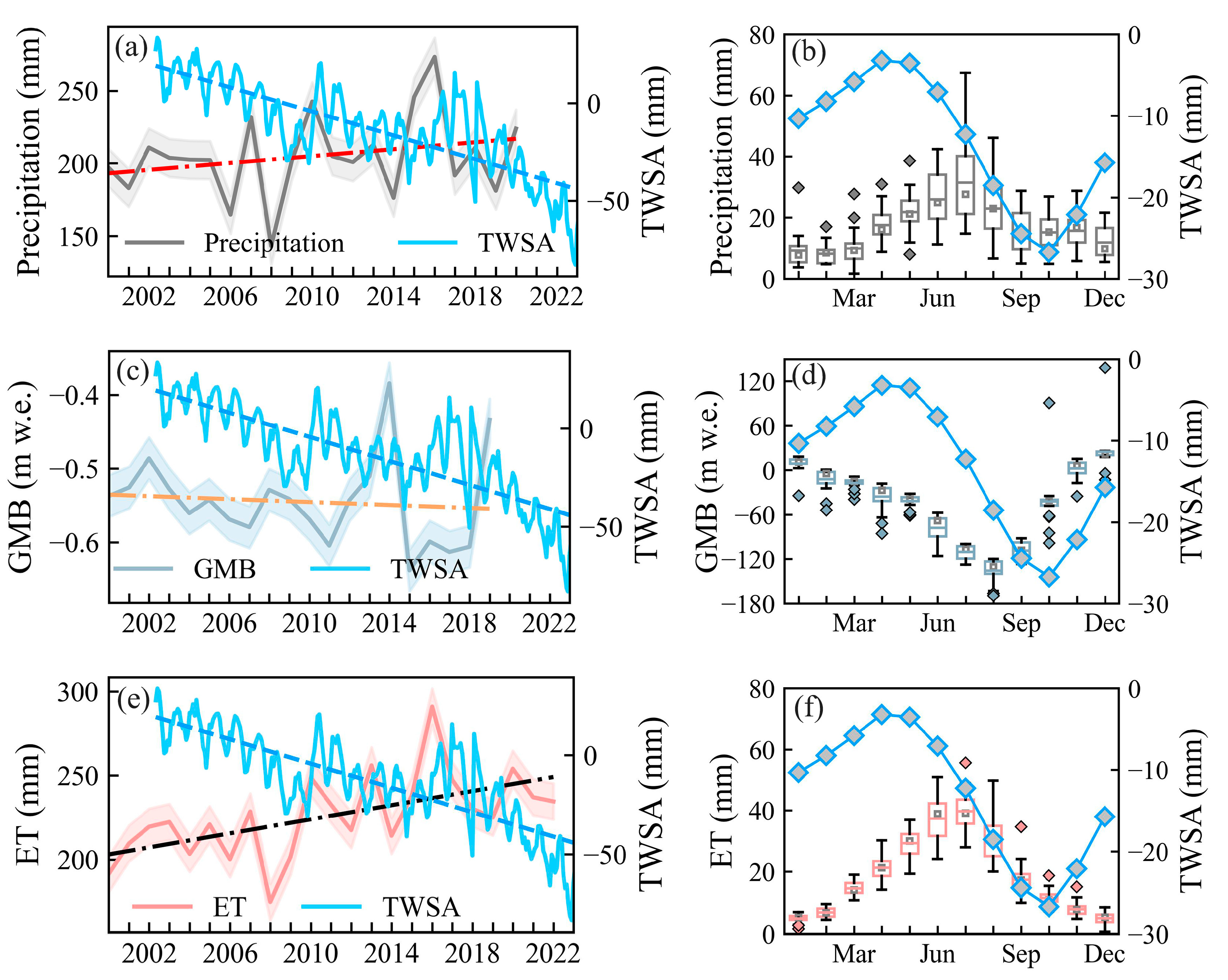
Since snow water, glacier meltwater, soil moisture, surface water and groundwater affect TWSA (with canopy water being negligible in the CMA (Figure S2)), we estimated each component's contribution to TWSA in the JBNWC and GLDWM regions separately. In both the JBNWC and GLDWM, GWSA is the primary contributor to TWSA variance, accounting for 78.16% and 90.28%, respectively, followed by SWEA at 18.61% and 6.04%. This indicates that TWSA variation is largely driven by fluctuations in groundwater reserves. A comparison of the GWSA, SWEA and TWSA time series reveals the three-month lag effect of GWSA and SWEA on TWSA in the JBNWC; this is due to delayed effects from snowmelt and groundwater recharge processes. In the GLDWM, although SWEA occasionally aligned with TWSA, a time lag of approximately 1–2 months was identified. In contrast, no lag was observed between GWSA and TWSA, as limited surface water resources in the GLDWM indicate that TWSA changes primarily reflect groundwater fluctuations. Our results showed that glaciers in the JBNWC and GLDWM experienced accelerated shrinkage during the study period, with glacier mass balance rates of -0.001 m w.e./yr and 0.01 m w.e./yr (Figure 8b-Figure 9b), respectively, which also explains the negative TWSA. These estimates were derived from a globally complete and consistent analysis of glacier mass change based on satellite observations, aligning with findings from previous research [57,82].
3.3. Spatial Dynamics of TWSA and GWSA
The spatial distribution of TWSA in the CMA, derived from three GRACE mascon solutions, reveals a consistent pattern, with the lowest values located in the southwestern region of the study area (Figure S4). As shown in Figure 6a, the spatially averaged annual mean TWSA derived from GRACE(-FO) indicates that the majority of the CMA (89.11%) experiences negative TWSA over the study period, reflecting TWSA deficits. The NTRB of the JBNWC exhibits the lowest TWSA at -147.34 mm. A significant decreasing trend in TWSA was detected across 98.61% of the CMA during this period (Figure 6b-6c, Figure S5), with the NTRB of the JBNWC showing the most substantial decline at a rate of -28.39 mm/yr. Compared to the JBNWC, the TWSA in the GLDWM exhibits a relatively uniform spatial distribution, with minimal spatial heterogeneity. Notably, the glacier-covered area in the KRB shows the most significant decreasing trend, at 13.37 mm/year. These findings suggest that glacier retreat in Mongolia's Altai Mountains has accelerated in recent years, likely driven by climate warming [83]. In addition, positive TWSA values are observed in the IRB, URB and ERB of the JBNWC, as well as in the KRB and BRB of the GLDWM, with the IRB of the JBNWC showing the highest TWSA at 30.38 mm. Notably, only the IRB and BRB exhibit significant increasing TWSA trends, at rates of 3.67 mm/yr and 2.84 mm/yr, respectively (Figure 6b-6c). Unlike TWSA, the maximum values and increasing trends of GWSA are observed in the KRB and BRB, whereas the GWSA in the IRB and URB shows negative values with a declining trend (Figure 6d–6f). This indicates that the rapid socioeconomic development in the JBNWC has led to a higher water demand, resulting in a significant reliance on groundwater resources. In contrast, in the GLDWM, glacier meltwater significantly recharges groundwater, resulting in an increase in groundwater storage.
As presented in Figure 7, the trends in TWSA and GWSA were analyzed across four seasons—spring, summer, autumn and winter. NTRB in the JBNWC experienced a significant decrease in TWSA and GWSA during spring, with the lowest values of -28.14 and -33.35 mm/yr, respectively, followed by summer and autumn, and decreased the least in winter. This highlights that agricultural irrigation in the JBNWC requires substantial water resources. However, the limited glacier-snow meltwater and precipitation are insufficient in meeting irrigation demands, making groundwater the primary source. Compared to the JBNWC, the GLDWM exhibits smaller seasonal variations in TWSA. However, the increases in GWSA within the KRB and BRB are most pronounced during winter and spring, followed by summer and autumn. This is attributed to the combined effects of glacier-snow meltwater and lower evaporation during winter and spring, which enhance groundwater recharge. In contrast, higher evaporation rates and increased human water demand during summer and autumn lead to relatively lower groundwater recharge.
3.4. Climatic and Anthropogenic Contributions to TWSA Dynamics
3.4.1. Climatic Factors
To assess the influential factors of climate-driven TWSA, multiple climate variables in the JBNWC and GLDWM have been analyzed. Figure 8 and Figure 9 depict the temporal variations in monthly TWSA, in comparison to precipitation, glacier and ET. The TWSA peak in the JBNWC occurs in April, while in the GLDWM, it remains relatively high throughout the winter and spring. In both regions, TWSA peaks occur earlier than the precipitation peak in July. Additionally, the summer evapotranspiration peak aligns with the precipitation peak, offsetting much of the water recharge from precipitation. This suggests that summer precipitation contributes only limited direct recharge to TWSA in the CMA region. In contrast, TWSA variations show a strong correlation with changes in glacier mass balance, indicating that meltwater from glaciers and snowmelt serves as the primary source of TWSA recharge in the CMA region[37,84]. Notably, the TWSA in JBNWC remains negative throughout the year, indicating a persistent water deficit in the region. This suggests that winter precipitation, glacier and snowmelt recharge are insufficient in meeting the region's water demand, thereby exacerbating groundwater depletion. Moreover, climate warming accelerates glacier retreat and increases evapotranspiration, further exacerbating the potential threats to regional water resources. Compared to the JBNWC, the TWSA in the GLDWM exceeds zero during the winter and spring, indicating that the region temporarily achieves water resource balance during these seasons. However, this balance is highly dependent on glacier meltwater recharge, and the long-term decline in glacier mass balance threatens to disrupt this seasonal equilibrium, posing significant risks and challenges to regional water resources in the future.
Figure 8.
Spatial distribution of TWSA trends (left panel) and GWSA trends (right panel) over four seasons: (a) and (e) MAM, (b) and (f) JJA, (c) and (g) SON and (d) and (h) DJF.
Figure 8.
Spatial distribution of TWSA trends (left panel) and GWSA trends (right panel) over four seasons: (a) and (e) MAM, (b) and (f) JJA, (c) and (g) SON and (d) and (h) DJF.
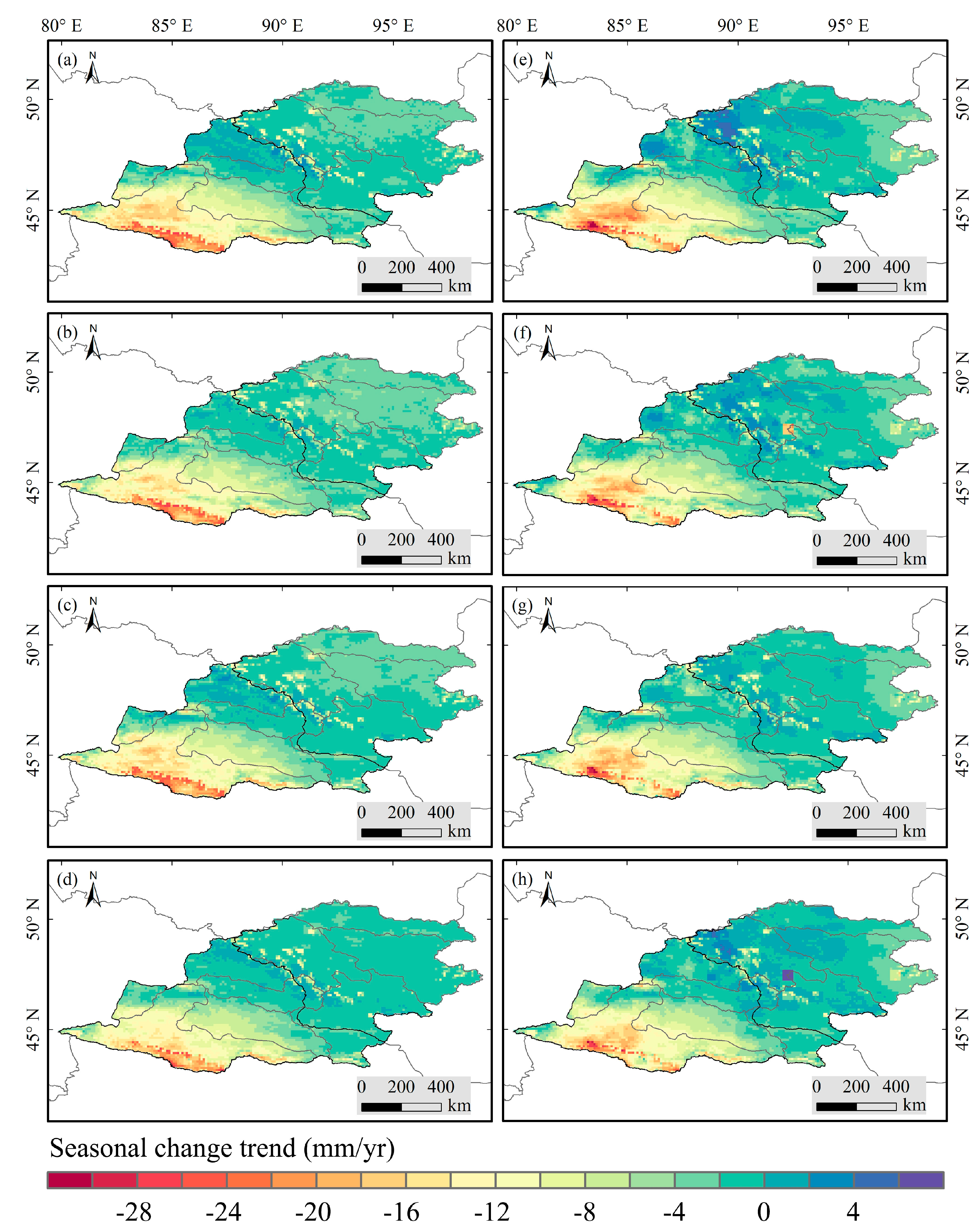
Figure 9.
Interannual and intra-annual variations of TWSA, precipitation, Glacier mass balance, and ET in JBNWC. GMB refers to glacier mass balance.
Figure 9.
Interannual and intra-annual variations of TWSA, precipitation, Glacier mass balance, and ET in JBNWC. GMB refers to glacier mass balance.
3.4.2. Anthropological Factor
To identify the anthropogenic drivers of TWSA variations, we analyzed the differences between GRACE and GLDAS data for the JBNWC and GLDWM. Figure 10a and Figure 10b illustrate these differences in the two regions, with RMSE values of 32.5 and 16.4, respectively. Notably, the TWSA trends from GRACE and GLDAS show relatively good consistency in both the JBNWC and GLDWM prior to 2010 (pre-2010), compared to the period thereafter (post-2010) (Figure 10a and Figure 10b). Since GLDAS primarily simulates TWSA variations driven by natural factors [100], this suggests that natural factors were the dominant contributors to TWSA changes before 2010. However, a significant increase in the inconsistency between GRACE and GLDAS is observed post-2010, with the RMSE increasing by 88.5% in the JBNWC and 34.5% in the GLDWM (Figure 10c). This substantial rise in discrepancy implies a shift in the dominant drivers of TWSA variations, possibly indicating the growing influence of anthropogenic factors. In the pre-2010 period, the TWSA trends derived from GRACE and GLDAS were -3.87 mm/yr and -0.25 mm/yr in the JBNWC, and -2.31 mm/yr and -1.42 mm/yr in the GLDWM, respectively (Figure 10d and Figure 10e). The underestimation of the declining TWSA trend in GLDAS is likely due to its exclusion of anthropogenic influences and its limited representation of water storage capacity [85]. This suggests that the observed TWSA decline during this period was primarily driven by climatic factors. In contrast, after 2010, the TWSA trends derived from GRACE showed a continued decrease (-3.95 mm/yr and -0.42 mm/yr) in both the JBNWC and GLDWM, while GLDAS showed an increasing trend (0.91 mm/yr and 1.1 mm/yr). Given that GLDAS primarily reflects climate-driven changes in TWSA, these results imply that the TWSA decline after 2010 was likely more influenced by anthropogenic activities than by natural factors.
Additionally, we analyzed the contributions of water withdrawals to shifts in the driving factors of TWSA changes. Figure 10f and Figure 10g show that water withdrawals increased by 10.19% in the JBNWC and 14.79% in the GLDWM from pre- to post-2010. This significant rise in water withdrawals further underscores the growing dominance of anthropogenic activities in the decline of TWSA, suggesting a shift from climate- to human-driven factors. It is important to note that, following the government’s implementation of efficient water-saving agricultural practices [86], water withdrawals in the JBNWC have been effectively controlled and gradually reduced since 2010. In contrast, although water withdrawal intensity in the GLDWM remains relatively low, the intensity of agricultural development, particularly in terms of water and land resource use, has been steadily increasing in recent years [87], leading to a continuous rise in water withdrawal intensity. Given the region's ecological vulnerability, the combined impacts of climate change and human activities are likely to exacerbate the conflict between water supply and demand in the future.
3.4.3. Relative Contributions of Drivers to the TWSA Trend
In this study, we employed STL decomposition to separate the inter-annual and seasonal components of TWSA as natural TWSA, while defining the linear trend and sub-seasonal residuals of TWSA as anthropogenic TWSA. Figure 11 illustrates the relative contributions of climate change and human activities to TWSA trends in the JBNWC and GLDWM over the 2002–2023 period. During this time, the natural TWSA variations in the JBNWC displayed fluctuating patterns, with climate change contributing 38.12% to the overall TWSA trend. In contrast, anthropogenic TWSA showed a marked declining trend (-0.26 mm/month), with human activities contributing 61.88% to the TWSA reduction. This significant decline highlights excessive groundwater depletion due to continued over-extraction, which was not adequately compensated by runoff from precipitation or glacier meltwater. In the GLDWM, natural TWSA variations were relatively smaller, with climate contributing 50.30% to the TWSA trend. The anthropogenic TWSA in this region also exhibited a downward trend (-0.09 mm/month), with human activities accounting for 49.70% of the TWSA reduction. Further analysis of the periods before and after 2010 revealed that, prior to 2010, TWSA decline in the JBNWC was driven by both climate change and human activities. However, in the GLDWM, climate change was the dominant driver (62.05%), with a lesser contribution from human activities (37.05%). Since 2010, the contribution of human activities to TWSA reduction has increased significantly, accounting for 70.36% in the JBNWC and 57.98% in the GLDWM, solidifying anthropogenic influences as the main factor driving TWSA decline (Figure 11c, f).
4. Discussion
4.1. Effect of Glacier Cover on GWSA
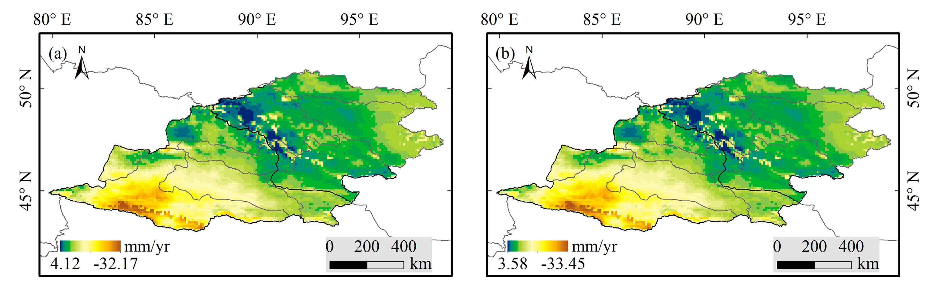
In glacier-covered regions, most previous studies estimating GWSA using the water storage components equation have directly ignored the presence of glaciers, resulting in groundwater storage change signals that are confounded with glacier change signals. To investigate the impact of glacier coverage on GWSA estimates, we examined the inter-annual trends of GWSA in different basins before and after glacier removal. There is no glacial development in the ERB, the Gurbantunggut Desert of the JBNWC, or the ULB of the GLDWM, so the trends in GWSA before and after glacier removal are identical (Table 2). For other basins, without removing glaciers, the GWSA estimates in glaciated areas actually represent the combined changes in groundwater and glaciers. For the NTRB of the JBNWC, since groundwater extraction is primarily concentrated in the plain and basin areas, the groundwater storage changes in the non-glaciated areas largely reflect those across the entire basin. In recent years, the Tianshan Mountains have experienced a significant loss in glacier mass, with melt causing a continuous decline in terrestrial water storage in the region [43,88]. As a result, the absolute rate of change in GWSA in the NTRB is slightly higher than that observed after removing glaciers, leading to an overestimation of 1.85%. In contrast, for the IRB of the JBNWC and the KRB of the GLDWM, located in the southern and northern slopes of the Altai Mountains, groundwater extraction is relatively low, and glacier recharge compensates for part of the groundwater depletion, resulting in underestimations of 24.98% and 17.78%, respectively. Additionally, although the glacier coverage in the URB of the JBNWC and the BRB and ZRB of the GLDWM are relatively small, there are still underestimations of 1.73%, 4.48%, and 4.42%, respectively. In terms of spatial variability, the spatial distributions of GWSA with and without glacier removal are nearly identical. Compared to the former, the GWSA decline rate in the glaciated areas of the NTRB is lower, while the increase rate in the KRB is higher, both highlighting the contribution of glaciers to groundwater recharge (Figure 12).
Figure 12.
The components of TWSA decomposed by STL in (a) JBNWC, (d) GLDWM; the anthropogenic activities dominated–TWS changes and climatic features dominated–TWS changes in (b) JBNWC, (e) GLDWM; Climatic and anthropogenic contributions on TWSA for the period 2002–2023 and subperiods 2002–2010 and 2011–2023 in (c) JBNWC, (f) GLDWM. EWT refers to equivalent water thickness.
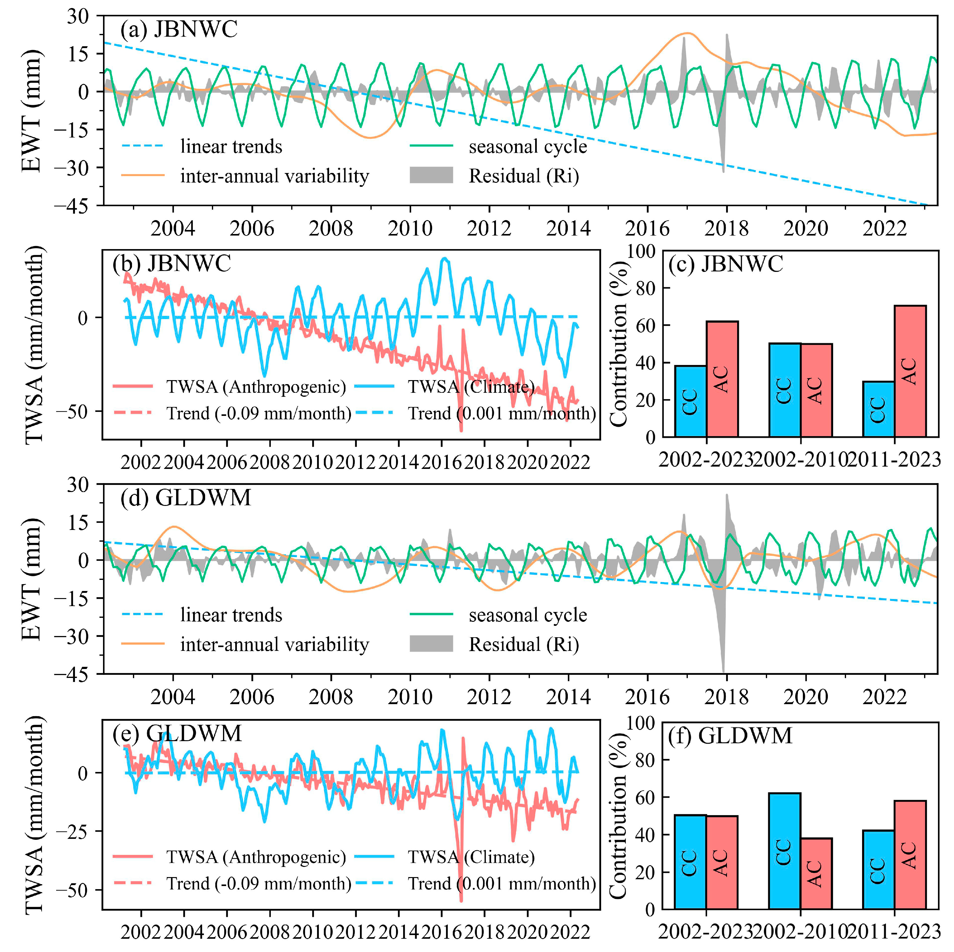
Figure 13.
Spatial distribution of interannual trends in GWSA before and after removal of glaciers.
4.2. Drivers of Water Storage Changes
Anthropogenic and climatic influences on changes in water storage are complex and non-linear, we compared the relative contributions of these two factors to TWS before and after 2010. Although annual precipitation in JBNWC is increasing (1.19 mm/yr), a larger rise (2.09 mm/yr) in evapotranspiration offsets the trend toward wetness (Figure 8a, e), leading to a warmer, drier climate [55]. With the implementation of China's Western Development Strategy, the economy of the JBNWC began to grow rapidly. From 2000 to 2010, the region's GDP was approximately CNY 1469.031 billion, and the sown area was 911,000 hectares (Figure S6). Economic expansion was largely driven by the extraction of abundant natural resources, including oil, natural gas and minerals, while agriculture and animal husbandry also played a supportive role in economic development. During this period, increased evaporation-induced drought played a dominant role in TWS decrease, with a climate-induced contribution rate of 55.71% (Table S1), relative to that of human activities (31.84%). From 2010 to 2021, the JBNWC experienced substantial economic growth, with GDP soaring by approximately 308.64% and sown area nearly doubling. Water withdrawal intensity rose by 10.19% (Table S1). To prevent the over-extraction of groundwater, the government implemented a series of policies and regulations, including shutting down illegal or non-compliant groundwater wells. Despite these efforts mitigating the decline in groundwater levels, the surging economy may continue to escalate water demand. Consequently, human activities contribute 70.36% to TWS reduction. Meanwhile, from 2010 to 2021, intensifying droughts accelerated glacier melting, replenishing regional water resources and reducing the contribution of climate change to TWS reduction to 27.54% (Table S1). The annual precipitation increase in GLDWM (1.42 mm/yr) slightly exceeds that of ET (1.34 mm/yr), but since annual ET surpasses annual precipitation (Figure 9a,e), the GLDWM is also becoming warmer and drier [89]. Compared to the JBNWC, the GLDWM's economic development remains in its early stages, relying on livestock farming and resource extraction. From 2000 to 2010, climate change drove 65.21% of TWS reduction (Table S1). To ensure food security, Mongolia has expanded arable land significantly since 2010, with sown areas and fodder crop cultivation increasing alongside rising livestock numbers to address extreme climate conditions. Industrial growth has also accelerated due to intensified mineral extraction. Since 2010, human activities have dominated TWS reduction, contributing 58.22%, which is slightly above climate change's 42.68% (Table S1).
Under the Belt and Road Initiative, the strategic importance of the CMA is growing, but water scarcity continues to be a significant constraint on the region's economic development. A thorough understanding of the water shortages in the area is crucial, as is the need to propose effective water resource management strategies. For the GLDWM, potential solutions include regulating livestock populations, promoting industrial diversification, and expanding the use of water-saving irrigation technologies. In the JBNWC, building a water-conserving society and implementing inter-basin water transfer projects offer feasible strategies to mitigate the water crisis.
4.3. Limitations and Future Work
This study does not explicitly account for the effects of mineral extraction and reservoir operations on TWS and GWS variability, which may introduce mass loss interference and lead to an overestimation of TWS changes. The lack of long-term, high-resolution datasets on mineral resource extraction limits our ability to accurately assess the spatiotemporal variation in TWS on a monthly scale. While the impact of mineral extraction on TWS trends is relatively minor, removing its influence could improve the accuracy of seasonal estimates. Future studies could explore potential vulnerabilities by projecting TWS using advanced climate models (e.g., CMIP6) to gain a deeper understanding of how water storage changes might affect food and water security in the CMA.
5. Conclusions
We examined GRACE-based water storage trends and possible drivers of variation to gain insights into how climate and human factors are linked to water storage variability. We used the RF model combined with residual correction, which exhibited superior performance compared to the RF model alone in predicting TWS and GWS anomalies. While TWS and GWS have durably decreased since 2002 over the majority of the CMA, the declining trends were more pronounced in areas with higher agricultural and human settlement impacts. We quantified the relative contributions of human activities and climate change to TWS dynamics and examined the influences of their driving factors. Although increased precipitation positively impacts TWS, the rise in evapotranspiration may accelerate its decline, partially offsetting these benefits, while glacier melting driven by climate change further accelerates TWS depletion. In the JBNWC, human activities such as increased sown area, water consumption, and settlements played dominant roles in TWS decrease. Compared with climate change (38.12%), the human-induced contribution rate was 61.88%, which increased to 70.36% after 2010. In the GLDWM, the primary driver of TWS decline shifted from climatic (2002-2010) to anthropogenic factors (2011-2020), while the contribution of human activities—such as the expansion of mineral extraction and sown area—increased from 37.95% to 57.98%. In addition, this study assessed the impact of glacial meltwater on GWS estimates, showing that neglecting it can lead to over- or underestimations across basins. Introducing advanced technology and controlling livestock in the GLDWM, while developing a water-saving society and implementing inter-basin water transfers in JBNWC, are viable strategies in addressing the water resource crisis. The presented framework is applicable to other regions for assessing local water resource vulnerabilities and developing effective management strategies.
Supplementary Materials
The following supporting information can be downloaded at the website of this paper posted on Preprints.org. Figure S1: title; Table S1: title; Video S1: title.
Author Contributions
Conceptualization, H.Z.; methodology, Y.Y.; software, Y.Y.; validation, S.W. and L.Y.; formal analysis, Y.S. and Y.Y.; investigation, D.B.; resources, D.B.; data curation, Y.S.; writing—original draft preparation, Y.Y.; writing—review and editing, Y.S., S.W and L.Y.; visualization, Y.Y and L.Y.; supervision, W.M.; project administration, H.Z.; funding acquisition, H.Z. All authors have read and agreed to the published version of the manuscript.
Funding
This research was funded by the National Key Research and Development Project of China (grant No. 2022YFE0119400) and the Science &Technology Fundamental Resources Investigation Program (Grant NO.2023FY100701).
Data Availability Statement
The original contributions presented in the study are included in the article, further inquiries can be directed to the corresponding author.
Conflicts of Interest
The authors declare no conflict of interest.
References
- Rodell, M.; Famiglietti, J.S. An Analysis of Terrestrial Water Storage Variations in Illinois with Implications for the Gravity Recovery and Climate Experiment (GRACE). Water Resour. Res. 2001, 37, 1327–1339. [Google Scholar] [CrossRef]
- Tapley, B.D.; Watkins, M.M.; Flechtner, F.; Reigber, C.; Bettadpur, S.; Rodell, M.; Sasgen, I.; Famiglietti, J.S.; Landerer, F.W.; Chambers, D.P.; et al. Contributions of GRACE to Understanding Climate Change. Nat. Clim. Change 2019, 9, 358–369. [Google Scholar] [CrossRef]
- Immerzeel, W.W.; Lutz, A.F.; Andrade, M.; Bahl, A.; Biemans, H.; Bolch, T.; Hyde, S.; Brumby, S.; Davies, B.J.; Elmore, A.C.; et al. Importance and Vulnerability of the World’s Water Towers. Nature 2020, 577, 364–369. [Google Scholar] [CrossRef] [PubMed]
- Long, D.; Longuevergne, L.; Scanlon, B.R. Uncertainty in Evapotranspiration from Land Surface Modeling, Remote Sensing, and GRACE Satellites. Water Resour. Res. 2014, 50, 1131–1151. [Google Scholar] [CrossRef]
- Scanlon, B.R.; Zhang, Z.; Save, H.; Wiese, D.N.; Landerer, F.W.; Long, D.; Longuevergne, L.; Chen, J. Global Evaluation of New GRACE Mascon Products for Hydrologic Applications. Water Resour. Res. 2016, 52, 9412–9429. [Google Scholar] [CrossRef]
- Chen, Y.; Zhang, X.; Fang, G.; Li, Z.; Wang, F.; Qin, J.; Sun, F. Potential Risks and Challenges of Climate Change in the Arid Region of Northwestern China. Reg. Sustainability 2020, 1, 20–30. [Google Scholar] [CrossRef]
- Li, H.; Hu, Y. Batunacun Responses of Vegetation Low-Growth to Extreme Climate Events on the Mongolian Plateau. Global Ecol. Conserv. 2024, 56, e03292. [Google Scholar] [CrossRef]
- Li, X.; Dong, W.; Liu, Y.; Yang, Y. Tracking the Urban Expansion and Its Driving Mechanisms behind Xinjiang Production and Construction Corps (XPCC): Evidence from Morphology and Landscapes. Habitat Int. 2022, 126, 102599. [Google Scholar] [CrossRef]
- Avirmed, D. Mineral Resources of Mongolia as a Driving Force of the Country. Mong. j. int. aff. 2021, 61–66. [Google Scholar] [CrossRef]
- Erdenechimeg, E.; Asralt, B.; Khurelbaatar, G. Distribution of Mongolian Mineral Resources, Transportation and Logistics Analysis; Asian Infrastructure Research Institute, Transportation Department, MTS of Mongolian University of Science and Technology: Ulaanbaatar, Mongolia, 2019. [Google Scholar]
- Hu, Z.; Zhang, Z.; Sang, Y.-F.; Qian, J.; Feng, W.; Chen, X.; Zhou, Q. Temporal and Spatial Variations in the Terrestrial Water Storage across Central Asia Based on Multiple Satellite Datasets and Global Hydrological Models. J. Hydrol. 2021, 596, 126013. [Google Scholar] [CrossRef]
- Pokhrel, Y.; Felfelani, F.; Satoh, Y.; Boulange, J.; Burek, P.; Gädeke, A.; Gerten, D.; Gosling, S.N.; Grillakis, M.; Gudmundsson, L.; et al. Global Terrestrial Water Storage and Drought Severity under Climate Change. Nat. Clim. Chang. 2021, 11, 226–233. [Google Scholar] [CrossRef]
- Liu, M.; Pei, H.; Shen, Y. Evaluating Dynamics of GRACE Groundwater and Its Drought Potential in Taihang Mountain Region, China. J. Hydrol. 2022, 612, 128156. [Google Scholar] [CrossRef]
- Wang, Y.; Li, C.; Cui, Y.; Cui, Y.; Xu, Y.; Hora, T.; Zaveri, E.; Rodella, A.-S.; Bai, L.; Long, D. Spatial Downscaling of GRACE-Derived Groundwater Storage Changes across Diverse Climates and Human Interventions with Random Forests. Journal of Hydrology 2024, 640, 131708. [Google Scholar] [CrossRef]
- Li, W.; Reichstein, M.; O, S.; May, C.; Destouni, G.; Migliavacca, M.; Kraft, B.; Weber, U.; Orth, R. Contrasting Drought Propagation into the Terrestrial Water Cycle between Dry and Wet Regions. Earth’s Future 2023, 11, e2022EF003441. [Google Scholar] [CrossRef]
- Yang, B.; Cui, Q.; Meng, Y.; Zhang, Z.; Hong, Z.; Hu, F.; Li, J.; Tao, C.; Wang, Z.; Zhang, W. Combined Multivariate Drought Index for Drought Assessment in China from 2003 to 2020. Agricultural Water Management 2023, 281, 108241. [Google Scholar] [CrossRef]
- Pan, Y.; Ding, H.; Li, J.; Shum, C.K.; Mallick, R.; Jiao, J.; Li, M.; Zhang, Y. Transient Hydrology-Induced Elastic Deformation and Land Subsidence in Australia Constrained by Contemporary Geodetic Measurements. Earth and Planetary Science Letters 2022, 588, 117556. [Google Scholar] [CrossRef]
- Sun, A.Y.; Scanlon, B.R.; Save, H.; Rateb, A. Reconstruction of GRACE Total Water Storage through Automated Machine Learning. Water Resources Research 2021, 57, e2020WR028666. [Google Scholar] [CrossRef]
- Yin, W.; Zhang, G.; Han, S.-C.; Yeo, I.-Y.; Zhang, M. Improving the Resolution of GRACE-Based Water Storage Estimates Based on Machine Learning Downscaling Schemes. J. Hydrol. 2022, 613, 128447. [Google Scholar] [CrossRef]
- Zhang, X.; Wu, X.; Mu, W.; Zhao, R.; Ye, B.; Bai, Z. Understanding the Shift in Drivers of Terrestrial Water Storage Decline in the Central Inner Mongolian Steppe over the Past Two Decades. J. Hydrol. 2024, 636, 131312. [Google Scholar] [CrossRef]
- Akhtar, F.; Nawaz, R.A.; Hafeez, M.; Awan, U.K.; Borgemeister, C.; Tischbein, B. Evaluation of GRACE Derived Groundwater Storage Changes in Different Agro-Ecological Zones of the Indus Basin. Journal of Hydrology 2022, 605, 127369. [Google Scholar] [CrossRef]
- Long, D.; Longuevergne, L.; Scanlon, B.R. Global Analysis of Approaches for Deriving Total Water Storage Changes from GRACE Satellites. Water Resources Research 2015, 51, 2574–2594. [Google Scholar] [CrossRef]
- Pascal, C.; Ferrant, S.; Selles, A.; Maréchal, J.-C.; Paswan, A.; Merlin, O. Evaluating Downscaling Methods of GRACE (Gravity Recovery and Climate Experiment) Data: A Case Study over a Fractured Crystalline Aquifer in Southern India. Hydrol. Earth Syst. Sci. 2022, 26, 4169–4186. [Google Scholar] [CrossRef]
- Feng, W.; Zhong, M.; Lemoine, J.; Biancale, R.; Hsu, H.; Xia, J. Evaluation of Groundwater Depletion in North China Using the Gravity Recovery and Climate Experiment (GRACE) Data and Ground-based Measurements. Water Resources Research 2013, 49, 2110–2118. [Google Scholar] [CrossRef]
- Abowarda, A.S.; Bai, L.; Zhang, C.; Long, D.; Li, X.; Huang, Q.; Sun, Z. Generating Surface Soil Moisture at 30 m Spatial Resolution Using Both Data Fusion and Machine Learning toward Better Water Resources Management at the Field Scale. Remote Sensing of Environment 2021, 255, 112301. [Google Scholar] [CrossRef]
- Hutengs, C.; Vohland, M. Downscaling Land Surface Temperatures at Regional Scales with Random Forest Regression. Remote Sensing of Environment 2016, 178, 127–141. [Google Scholar] [CrossRef]
- Scanlon, B.R.; Zhang, Z.; Rateb, A.; Sun, A.; Wiese, D.; Save, H.; Beaudoing, H.; Lo, M.H.; Müller-Schmied, H.; Döll, P.; et al. Tracking Seasonal Fluctuations in Land Water Storage Using Global Models and GRACE Satellites. Geophysical Research Letters 2019, 46, 5254–5264. [Google Scholar] [CrossRef]
- Liu, Z. Causes of Changes in Actual Evapotranspiration and Terrestrial Water Storage over the Eurasian Inland Basins. Hydrological Processes 2022, 36, e14482. [Google Scholar] [CrossRef]
- Panda, D.K.; Wahr, J. Spatiotemporal Evolution of Water Storage Changes in India from the Updated GRACE-Derived Gravity Records. Water Resources Research 2016, 52, 135–149. [Google Scholar] [CrossRef]
- Joodaki, G.; Wahr, J.; Swenson, S. Estimating the Human Contribution to Groundwater Depletion in the Middle East, from GRACE Data, Land Surface Models, and Well Observations. Water Resources Research 2014, 50, 2679–2692. [Google Scholar] [CrossRef]
- Rateb, A.; Scanlon, B.R.; Pool, D.R.; Sun, A.; Zhang, Z.; Chen, J.; Clark, B.; Faunt, C.C.; Haugh, C.J.; Hill, M.; et al. Comparison of Groundwater Storage Changes from GRACE Satellites with Monitoring and Modeling of Major U.S. Aquifers. Water Resour. Res. 2020, 56, e2020WR027556. [Google Scholar] [CrossRef]
- Cheng, W.; Feng, Q.; Xi, H.; Yin, X.; Sindikubwabo, C.; Habiyakare, T.; Chen, Y.; Zhao, X. Spatiotemporal Variability and Controlling Factors of Groundwater Depletion in Endorheic Basins of Northwest China. Journal of Environmental Management 2023, 344, 118468. [Google Scholar] [CrossRef] [PubMed]
- Duan, L.; Chen, X.; Bu, L.; Chen, C.; Song, S. Temporal and Spatial Variation Analysis of Groundwater Stocks in Xinjiang Based on GRACE Data. Remote Sensing 2024, 16, 813. [Google Scholar] [CrossRef]
- Ma, X.; Wu, T.; Adiya, S.; Avirmed, D.; Zhu, X.; Shang, C.; Yan, X.; Lou, P.; Wang, D.; Chen, J.; et al. Spatiotemporal Variations of Permafrost Extent in Mongolia during 1950–2022. Ecological Indicators 2024, 166, 112558. [Google Scholar] [CrossRef]
- Walther, M.; Kamp, U. Mountain Permafrost: A Reflection on the Periglacial Environment in Mongolia. Geosciences 2023, 13, 274. [Google Scholar] [CrossRef]
- Kamp, U.; Walther, M.; Dashtseren, A. Mongolia’s Cryosphere. Geomorphology 2022, 410, 108202. [Google Scholar] [CrossRef]
- Tsutomu, K.; Gombo, D. Recent Glacier Variations in Mongolia. Ann. Glaciol. 2007, 46, 185–188. [Google Scholar] [CrossRef]
- Tao, S.; Fang, J.; Zhao, X.; Zhao, S.; Shen, H.; Hu, H.; Tang, Z.; Wang, Z.; Guo, Q. Rapid Loss of Lakes on the Mongolian Plateau. Proc. Natl. Acad. Sci. U.S.A. 2015, 112, 2281–2286. [Google Scholar] [CrossRef] [PubMed]
- Zhao, H.; Qiao, B.; Liu, H.; Chen, X.; Xiao, Y.; Wang, G. Lake Water Storage Changes and Their Cause Analysis in Mongolia. Sci Rep 2024, 14, 23536. [Google Scholar] [CrossRef]
- Li, Q.; Liu, X.; Zhong, Y.; Wang, M.; Bai, H.; Xiao, C. Assessing the Interannual and Subseasonal Variabilities in Water Storage Using Multi-Source Soil Moisture Products and GRACE/GRACE-FO Satellites and Its Applications. Journal of Hydrology 2023, 627, 130439. [Google Scholar] [CrossRef]
- Zheng, S.; Zhang, Z.; Song, Z.; Li, Y.; Yan, H. Anthropogenic and Climate-Driven Water Storage Variations on the Mongolian Plateau. Remote Sens. 2023, 15, 4184. [Google Scholar] [CrossRef]
- Arshad, A.; Mirchi, A.; Taghvaeian, S.; AghaKouchak, A. Downscaled-GRACE Data Reveal Anthropogenic and Climate-induced Water Storage Decline across the Indus Basin. Water Resour. Res. 2024, 60, e2023WR035882. [Google Scholar] [CrossRef]
- Deng, H.; Chen, Y. Influences of Recent Climate Change and Human Activities on Water Storage Variations in Central Asia. Journal of Hydrology 2017, 544, 46–57. [Google Scholar] [CrossRef]
- Zhang, Y.; He, B.; Guo, L.; Liu, J.; Xie, X. The Relative Contributions of Precipitation, Evapotranspiration, and Runoff to Terrestrial Water Storage Changes across 168 River Basins. J. Hydrol. 2019, 579, 124194. [Google Scholar] [CrossRef]
- Li, X.; Long, D.; Scanlon, B.R.; Mann, M.E.; Li, X.; Tian, F.; Sun, Z.; Wang, G. Climate Change Threatens Terrestrial Water Storage over the Tibetan Plateau. Nat. Clim. Change 2022, 12, 801–807. [Google Scholar] [CrossRef]
- Taylor, R.G.; Scanlon, B.; Döll, P.; Rodell, M.; Van Beek, R.; Wada, Y.; Longuevergne, L.; Leblanc, M.; Famiglietti, J.S.; Edmunds, M.; et al. Ground Water and Climate Change. Nat. Clim. Change 2013, 3, 322–329. [Google Scholar] [CrossRef]
- Han, Z.; Huang, S.; Huang, Q.; Bai, Q.; Leng, G.; Wang, H.; Zhao, J.; Wei, X.; Zheng, X. Effects of Vegetation Restoration on Groundwater Drought in the Loess Plateau, China. J. Hydrol. 2020, 591, 125566. [Google Scholar] [CrossRef]
- Xie, X.; Xu, C.; Wen, Y.; Li, W. Monitoring Groundwater Storage Changes in the Loess Plateau Using GRACE Satellite Gravity Data, Hydrological Models and Coal Mining Data. Remote Sens. 2018, 10, 605. [Google Scholar] [CrossRef]
- Xie, J.; Xu, Y.-P.; Wang, Y.; Gu, H.; Wang, F.; Pan, S. Influences of Climatic Variability and Human Activities on Terrestrial Water Storage Variations across the Yellow River Basin in the Recent Decade. J. Hydrol. 2019, 579, 124218. [Google Scholar] [CrossRef]
- Pei, H.; Liu, M.; Shen, Y.; Xu, K.; Zhang, H.; Li, Y.; Luo, J. Quantifying Impacts of Climate Dynamics and Land-Use Changes on Water Yield Service in the Agro-Pastoral Ecotone of Northern China. Science of The Total Environment 2022, 809, 151153. [Google Scholar] [CrossRef]
- Cao, Y.; Nan, Z.; Cheng, G.; Zhang, L. Hydrological Variability in the Arid Region of Northwest China from 2002 to 2013. Advances in Meteorology 2018, 2018, 1–13. [Google Scholar] [CrossRef]
- Meng, F.; Luo, M.; Sa, C.; Wang, M.; Bao, Y. Quantitative Assessment of the Effects of Climate, Vegetation, Soil and Groundwater on Soil Moisture Spatiotemporal Variability in the Mongolian Plateau. Sci. Total Environ. 2022, 809, 152198. [Google Scholar] [CrossRef]
- Yin, Z.; Xu, Y.; Zhu, X.; Zhao, J.; Yang, Y.; Li, J. Variations of Groundwater Storage in Different Basins of China over Recent Decades. Journal of Hydrology 2021, 598, 126282. [Google Scholar] [CrossRef]
- Zhu, E.; Wang, Y.; Yuan, X. Changes of Terrestrial Water Storage during 1981–2020 over China Based on Dynamic-Machine Learning Model. Journal of Hydrology 2023, 621, 129576. [Google Scholar] [CrossRef]
- Deng, H.; Tang, Q.; Yun, X.; Tang, Y.; Liu, X.; Xu, X.; Sun, S.; Zhao, G.; Zhang, Y.; Zhang, Y. Wetting Trend in Northwest China Reversed by Warmer Temperature and Drier Air. J. Hydrol. 2022, 613, 128435. [Google Scholar] [CrossRef]
- Li, Q.; Chen, Y.; Shen, Y.; Li, X.; Xu, J. Spatial and Temporal Trends of Climate Change in Xinjiang, China. J. Geogr. Sci 2011, 21, 1007–1018. [Google Scholar] [CrossRef]
- The Physical Geography of Mongolia; Yembuu, B, Ed.; Geography of the Physical Environment; Springer International Publishing: Cham, 2021; ISBN 978-3-030-61433-1. [Google Scholar]
- Tsegmid, S. Physical Geography of Mongolia; Mongolian Academy of Sciences, Institute of Geography and Permafrost: Mongolia, 1969; pp. 18–21. [Google Scholar]
- Cao, X.; Wu, N.; Adamowski, J.; Wu, M. Assessing the Contribution of China’s Grain Production during 2005–2020 from the Perspective of the Crop-Water-Land Nexus. J. Hydrol. 2023, 626, 130376. [Google Scholar] [CrossRef]
- Xu, Y.; Zhang, Y.; Chen, J.; John, R. Livestock Dynamics under Changing Economy and Climate in Mongolia. Land Use Policy 2019, 88, 104120. [Google Scholar] [CrossRef]
- Pokhrel, Y.; Felfelani, F.; Satoh, Y.; Boulange, J.; Burek, P.; Gädeke, A.; Gerten, D.; Gosling, S.N.; Grillakis, M.; Gudmundsson, L.; et al. Global Terrestrial Water Storage and Drought Severity under Climate Change. Nat. Clim. Chang. 2021, 11, 226–233. [Google Scholar] [CrossRef]
- Bhanja, S.N.; Zhang, X.; Wang, J. Estimating Long-Term Groundwater Storage and Its Controlling Factors in Alberta, Canada. Hydrol. Earth Syst. Sci. 2018, 22, 6241–6255. [Google Scholar] [CrossRef]
- Watkins, M.M.; Wiese, D.N.; Yuan, D.; Boening, C.; Landerer, F.W. Improved Methods for Observing Earth’s Time Variable Mass Distribution with GRACE Using Spherical Cap Mascons. J. Geophys. Res.: Solid Earth 2015, 120, 2648–2671. [Google Scholar] [CrossRef]
- Luthcke, S.B.; Sabaka, T.J.; Loomis, B.D.; Arendt, A.A.; McCarthy, J.J.; Camp, J. Antarctica, Greenland and Gulf of Alaska Land-Ice Evolution from an Iterated GRACE Global Mascon Solution. J. Glaciol. 2013, 59, 613–631. [Google Scholar] [CrossRef]
- Save, H.; Bettadpur, S.; Tapley, B.D. High-resolution CSR GRACE RL05 Mascons. J. Geophys. Res.: Solid Earth 2016, 121, 7547–7569. [Google Scholar] [CrossRef]
- Hugonnet, R.; McNabb, R.; Berthier, E.; Menounos, B.; Nuth, C.; Girod, L.; Farinotti, D.; Huss, M.; Dussaillant, I.; Brun, F.; et al. Accelerated Global Glacier Mass Loss in the Early Twenty-First Century. Nature 2021, 592, 726–731. [Google Scholar] [CrossRef] [PubMed]
- Muñoz-Sabater, J.; Dutra, E.; Agustí-Panareda, A.; Albergel, C.; Arduini, G.; Balsamo, G.; Boussetta, S.; Choulga, M.; Harrigan, S.; Hersbach, H.; et al. ERA5-Land: A State-of-the-Art Global Reanalysis Dataset for Land Applications. Earth Syst. Sci. Data 2021, 13, 4349–4383. [Google Scholar] [CrossRef]
- Stefanidis, K.; Varlas, G.; Papaioannou, G.; Papadopoulos, A.; Dimitriou, E. Trends of Lake Temperature, Mixing Depth and Ice Cover Thickness of European Lakes during the Last Four Decades. Sci. Total Environ. 2022, 830, 154709. [Google Scholar] [CrossRef] [PubMed]
- Miro, M.; Famiglietti, J. Downscaling GRACE Remote Sensing Datasets to High-Resolution Groundwater Storage Change Maps of California’s Central Valley. Remote Sens. 2018, 10, 143. [Google Scholar] [CrossRef]
- Vishwakarma, B.D.; Zhang, J.; Sneeuw, N. Downscaling GRACE Total Water Storage Change Using Partial Least Squares Regression. Sci. Data 2021, 8, 95. [Google Scholar] [CrossRef]
- Zhong, D.; Wang, S.; Li, J. Spatiotemporal Downscaling of GRACE Total Water Storage Using Land Surface Model Outputs. Remote Sens. 2021, 13, 900. [Google Scholar] [CrossRef]
- Yuan, R.-Q.; Chang, L.-L.; Gupta, H.; Niu, G.-Y. Climatic Forcing for Recent Significant Terrestrial Drying and Wetting. Adv. Water Resour. 2019, 133, 103425. [Google Scholar] [CrossRef]
- Woldesenbet, T.A.; Elagib, N.A.; Ribbe, L.; Heinrich, J. Hydrological Responses to Land Use/Cover Changes in the Source Region of the Upper Blue Nile Basin, Ethiopia. Sci. Total Environ. 2017, 575, 724–741. [Google Scholar] [CrossRef]
- Breiman, L. Random Forests. Machine Learning 2001, 45, 5–32. [Google Scholar] [CrossRef]
- Cleveland, R.B.; Cleveland, W.S.; McRae, J.E.; Terpenning, I. STL a Seasonal-Trend Decomposition Procedure Based on Loess. Journal of Official Statistics 1990, 6, 3–73. [Google Scholar]
- Frappart, F.; Ramillien, G.; Ronchail, J. Changes in Terrestrial Water Storage versus Rainfall and Discharges in the Amazon Basin. Int. J. Climatol. 2013, 33, 3029–3046. [Google Scholar] [CrossRef]
- Humphrey, V.; Gudmundsson, L.; Seneviratne, S.I. Assessing Global Water Storage Variability from GRACE: Trends, Seasonal Cycle, Subseasonal Anomalies and Extremes. Surv. Geophys. 2016, 37, 357–395. [Google Scholar] [CrossRef]
- Zhu, Y.; Liu, S.; Yi, Y.; Xie, F.; Grünwald, R.; Miao, W.; Wu, K.; Qi, M.; Gao, Y.; Singh, D. Overview of Terrestrial Water Storage Changes over the Indus River Basin Based on GRACE/GRACE-FO Solutions. Sci. Total Environ. 2021, 799, 149366. [Google Scholar] [CrossRef]
- Miro, M.; Famiglietti, J. Downscaling GRACE Remote Sensing Datasets to High-Resolution Groundwater Storage Change Maps of California’s Central Valley. Remote Sens. 2018, 10, 143. [Google Scholar] [CrossRef]
- Zhong, Y.; Zhong, M.; Mao, Y.; Ji, B. Evaluation of Evapotranspiration for Exorheic Catchments of China during the GRACE Era: From a Water Balance Perspective. Remote Sens. 2020, 12, 511. [Google Scholar] [CrossRef]
- Wang, Z.; Liu, S. Estimation and Spatiotemporal Evolution of Groundwater Storage on the Northern Slope of the Tianshan Mountains over the Past Three Decades. Acta Geogr. Sin 2023, 78, 1744–1763. [Google Scholar]
- Su, B.; Xiao, C.; Chen, D.; Huang, Y.; Che, Y.; Zhao, H.; Zou, M.; Guo, R.; Wang, X.; Li, X.; et al. Glacier Change in China over Past Decades: Spatiotemporal Patterns and Influencing Factors. Earth-Science Reviews 2022, 226, 103926. [Google Scholar] [CrossRef]
- Kamp, U.; Walther, M.; Dashtseren, A. Mongolia’s Cryosphere. Geomorphology 2022, 410, 108202. [Google Scholar] [CrossRef]
- Shen, Y.-J.; Shen, Y.; Guo, Y.; Zhang, Y.; Pei, H.; Brenning, A. Review of Historical and Projected Future Climatic and Hydrological Changes in Mountainous Semiarid Xinjiang (Northwestern China), Central Asia. Catena 2020, 187, 104343. [Google Scholar] [CrossRef]
- Scanlon, B.R.; Zhang, Z.; Save, H.; Sun, A.Y.; Müller Schmied, H.; Van Beek, L.P.H.; Wiese, D.N.; Wada, Y.; Long, D.; Reedy, R.C.; et al. Global Models Underestimate Large Decadal Declining and Rising Water Storage Trends Relative to GRACE Satellite Data. Proc. Natl. Acad. Sci. 2018, 115. [Google Scholar] [CrossRef]
- Pei, D.; Wen, Y.; Li, W.; Ma, Z.; Guo, L.; Zhang, J.; Liu, M.; Mu, X.; Wang, Z. Agricultural Water Rebound Effect and Its Driving Factors in Xinjiang, China. Agric. Water Manage. 2024, 304, 109086. [Google Scholar] [CrossRef]
- Chan, F.K.S.; Chen, J.; Li, P.; Wang, J.; Wang, J.; Zhu, Y. The Cross-Boundary of Land Degradation in Mongolia and China and Achieving Its Neutrality - Challenges and Opportunities. Ecological Indicators 2023, 151, 110311. [Google Scholar] [CrossRef]
- Farinotti, D.; Longuevergne, L.; Moholdt, G.; Duethmann, D.; Mölg, T.; Bolch, T.; Vorogushyn, S.; Güntner, A. Substantial Glacier Mass Loss in the Tien Shan over the Past 50 Years. Nature Geosci 2015, 8, 716–722. [Google Scholar] [CrossRef]
- Zhang, P.; Jeong, J.-H.; Yoon, J.-H.; Kim, H.; Wang, S.-Y.S.; Linderholm, H.W.; Fang, K.; Wu, X.; Chen, D. Abrupt Shift to Hotter and Drier Climate over Inner East Asia beyond the Tipping Point. Science 2020, 370, 1095–1099. [Google Scholar] [CrossRef]
Figure 1.
Overview of the study area. The black line refers to the CMA. The bars represent the types of land use in 2000, 2010 and 2020.
Figure 1.
Overview of the study area. The black line refers to the CMA. The bars represent the types of land use in 2000, 2010 and 2020.
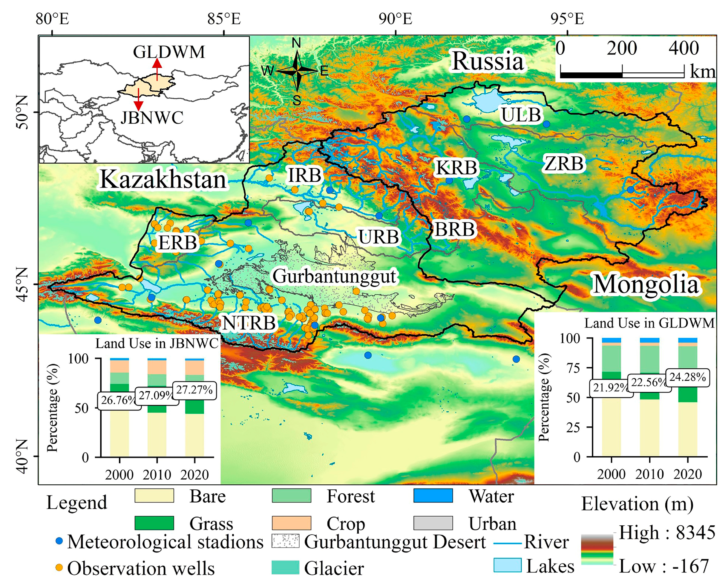
Figure 2.
Flowchart of this study.
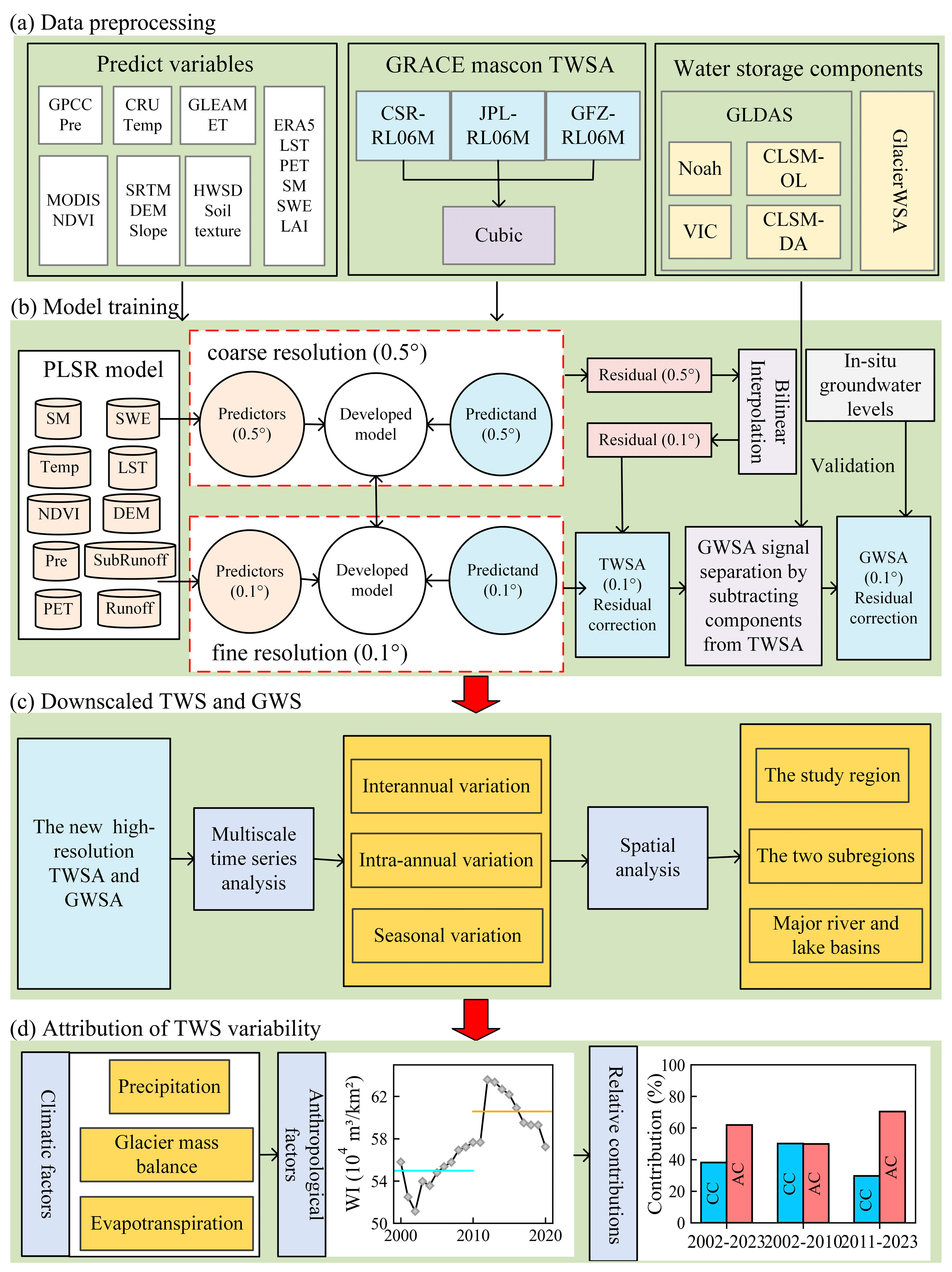
Figure 3.
VIP values of different predictors based on the PLSR model.
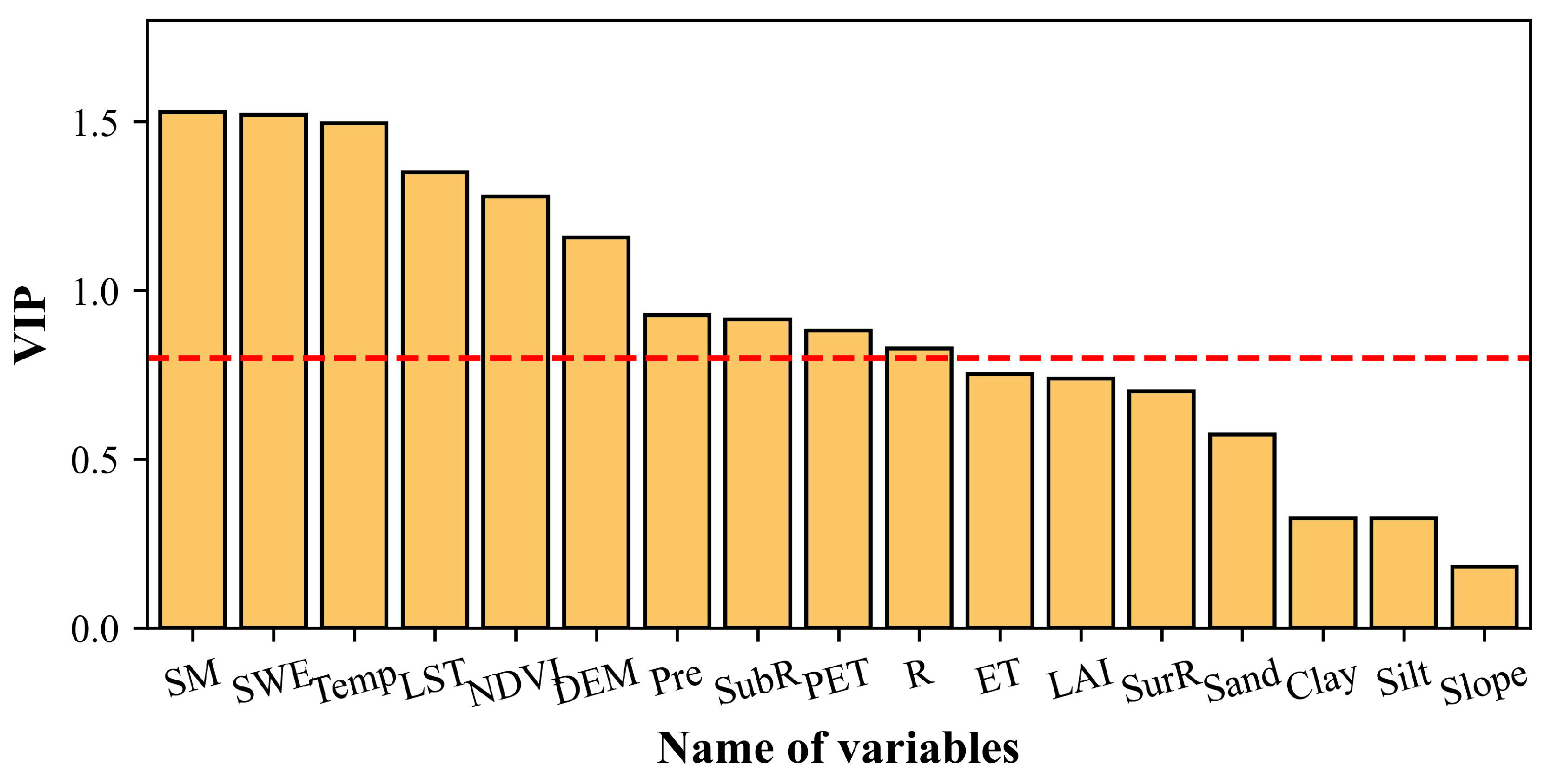
Figure 4.
Trends of TWSA and GWSA before and after downscaling during 2002–2023.
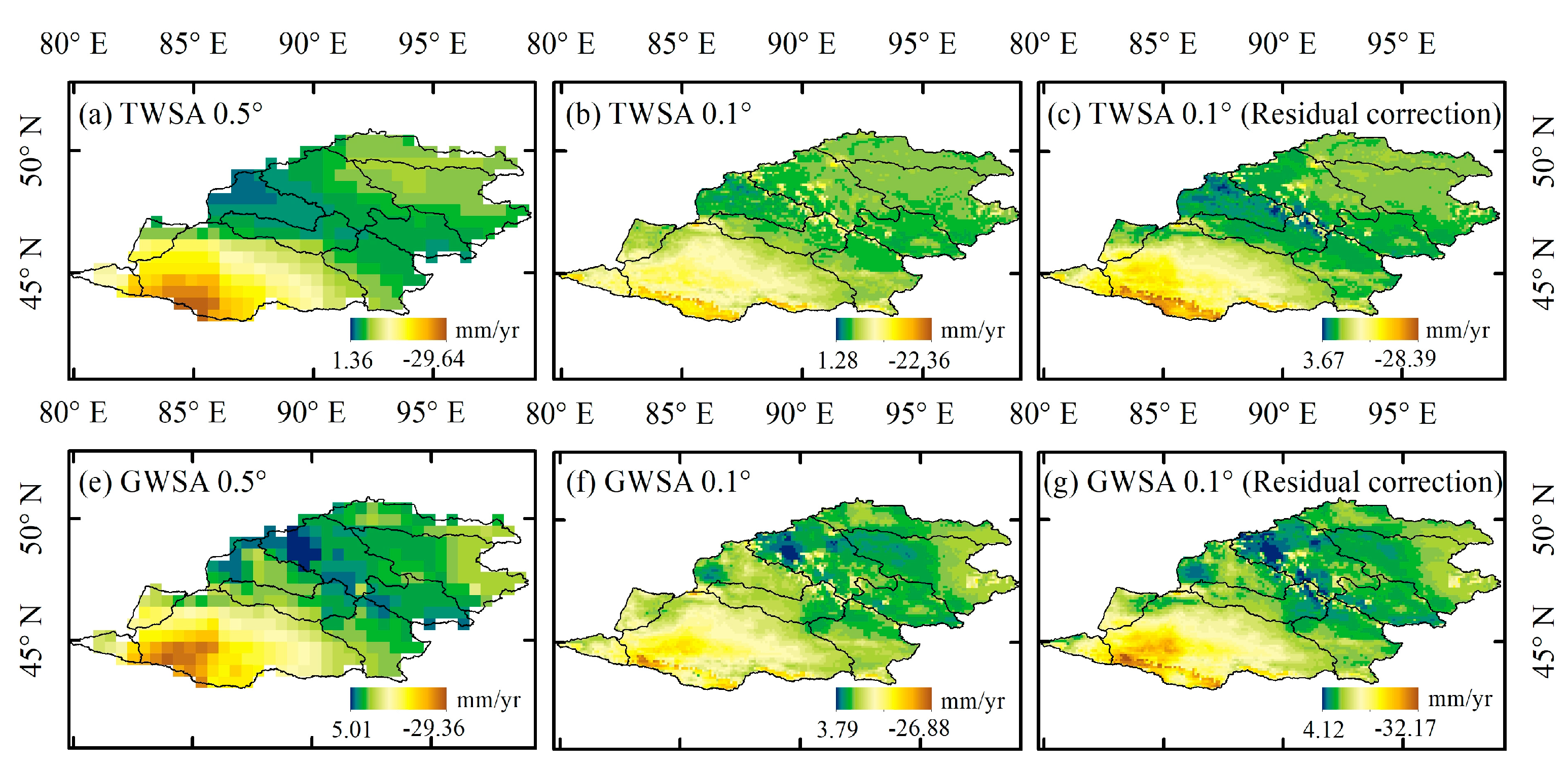
Figure 5.
(a) TWSA and (b) GWSA in the CMA during study period. Monthly mean and Yearly mean were given in the panel axes.
Figure 5.
(a) TWSA and (b) GWSA in the CMA during study period. Monthly mean and Yearly mean were given in the panel axes.
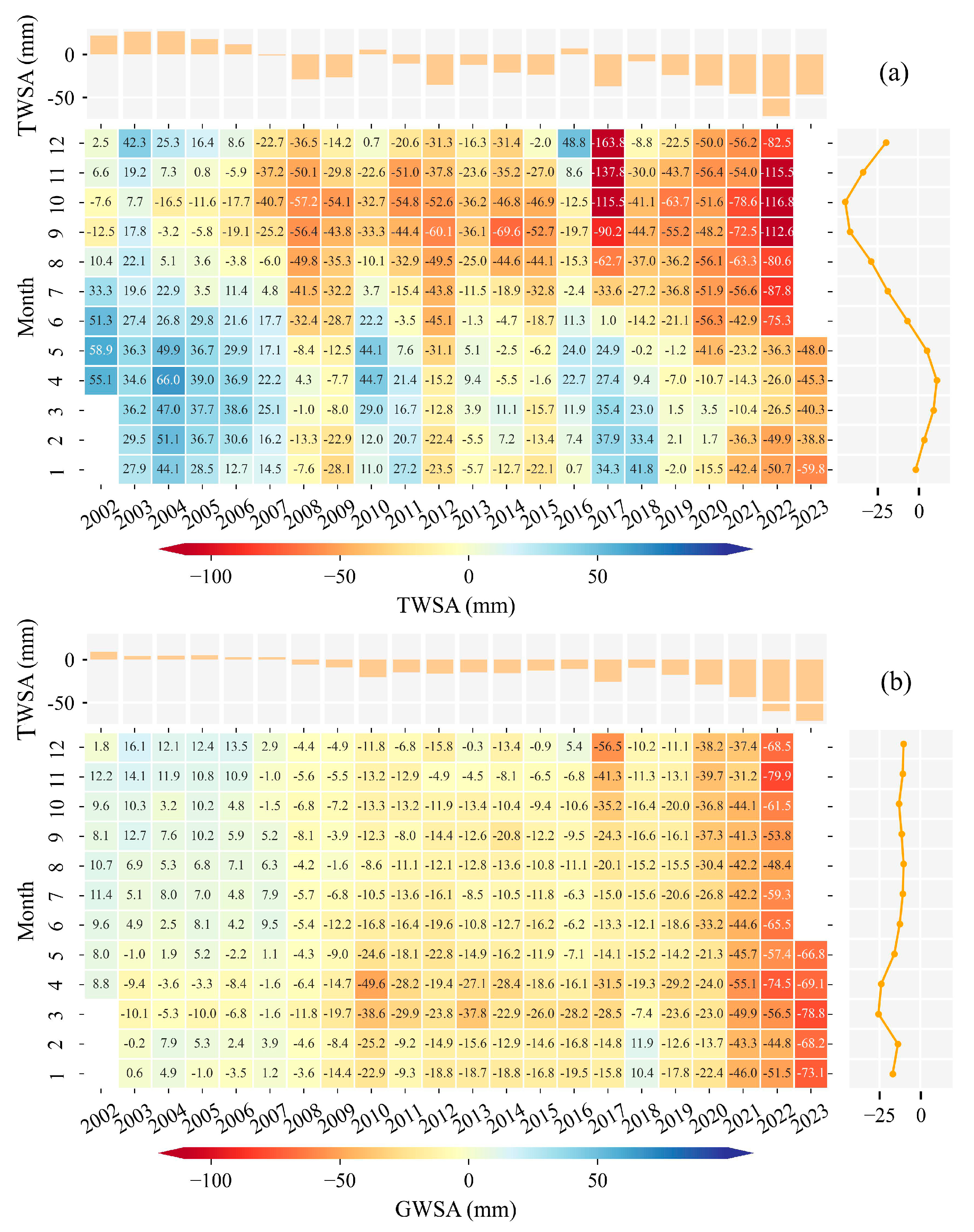
Figure 6.
Temporal variations of spatially averaged TWSA and its components over the CMA. EWT refers to equivalent water thickness.
Figure 6.
Temporal variations of spatially averaged TWSA and its components over the CMA. EWT refers to equivalent water thickness.
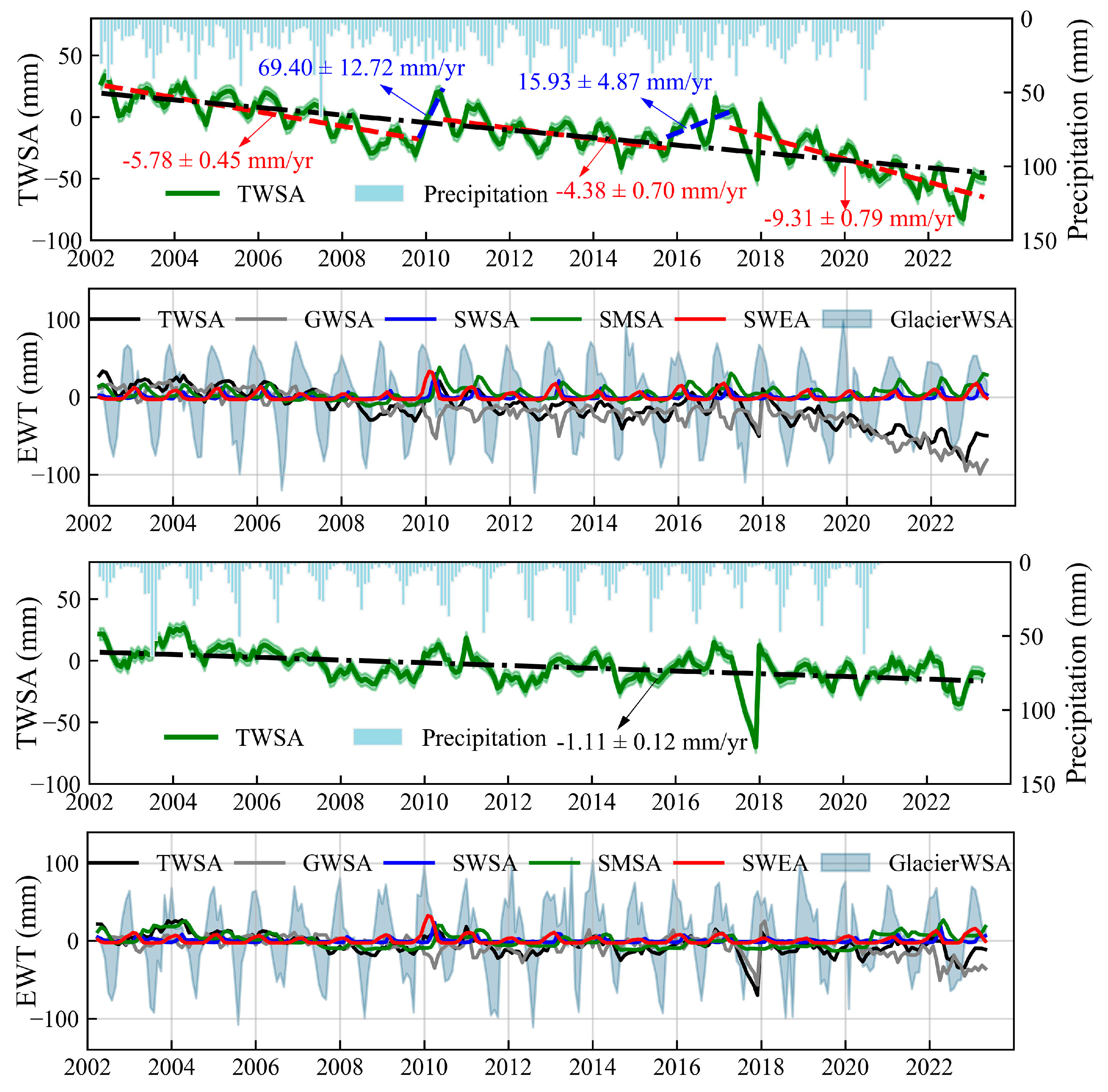
Figure 7.
Spatial characteristics of the TWSA and GWSA in the CMA. The spatial distribution of annual TWSA and GWSA was shown in (a), (d); the change rate was shown in (b), (e); the significance test results were shown in (c), (f).
Figure 7.
Spatial characteristics of the TWSA and GWSA in the CMA. The spatial distribution of annual TWSA and GWSA was shown in (a), (d); the change rate was shown in (b), (e); the significance test results were shown in (c), (f).
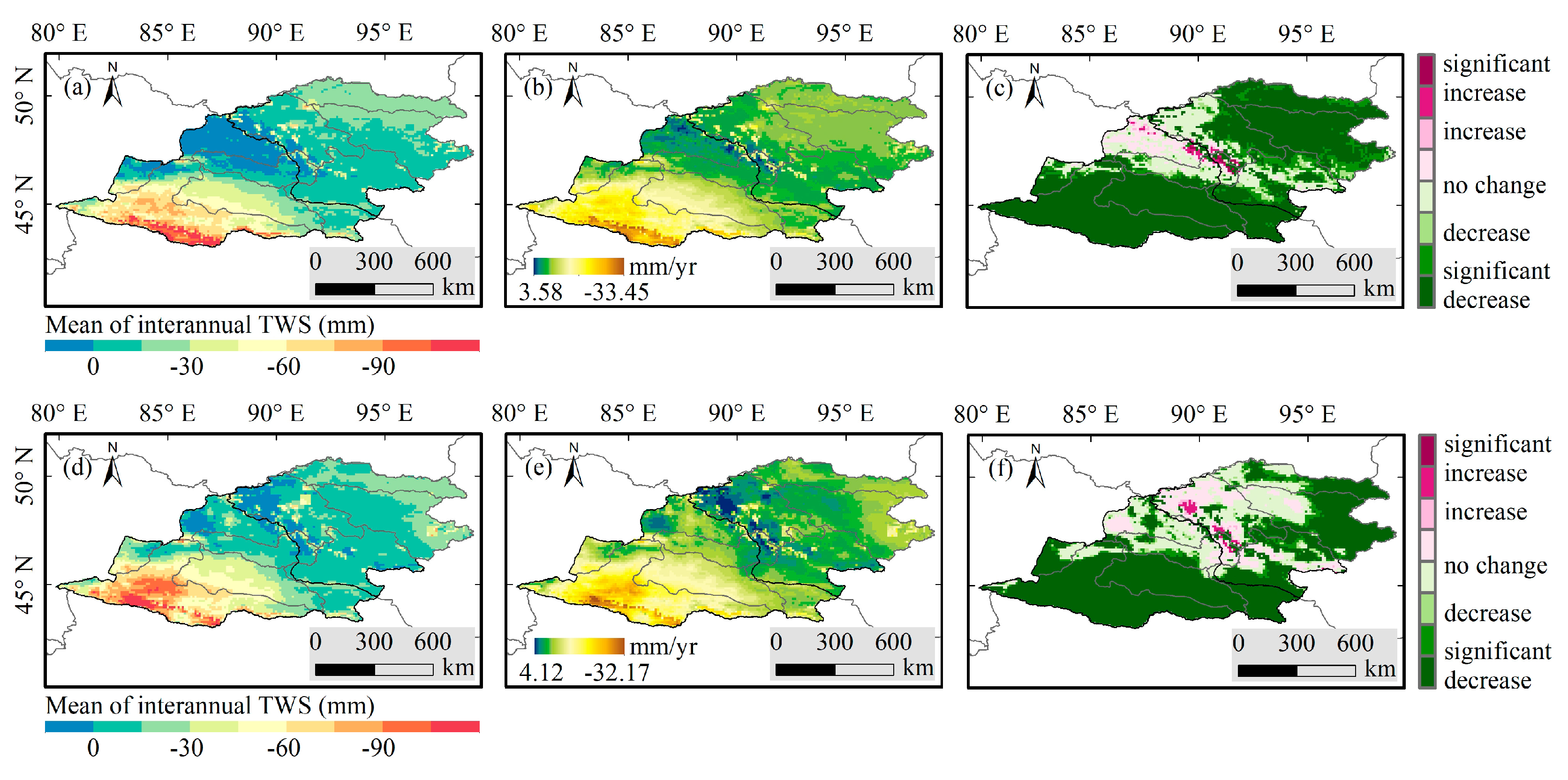
Figure 10.
Interannual and intra-annual variations of TWSA, precipitation, Glacier mass balance, and ET in GLDWM. GMB refers to glacier mass balance.
Figure 10.
Interannual and intra-annual variations of TWSA, precipitation, Glacier mass balance, and ET in GLDWM. GMB refers to glacier mass balance.
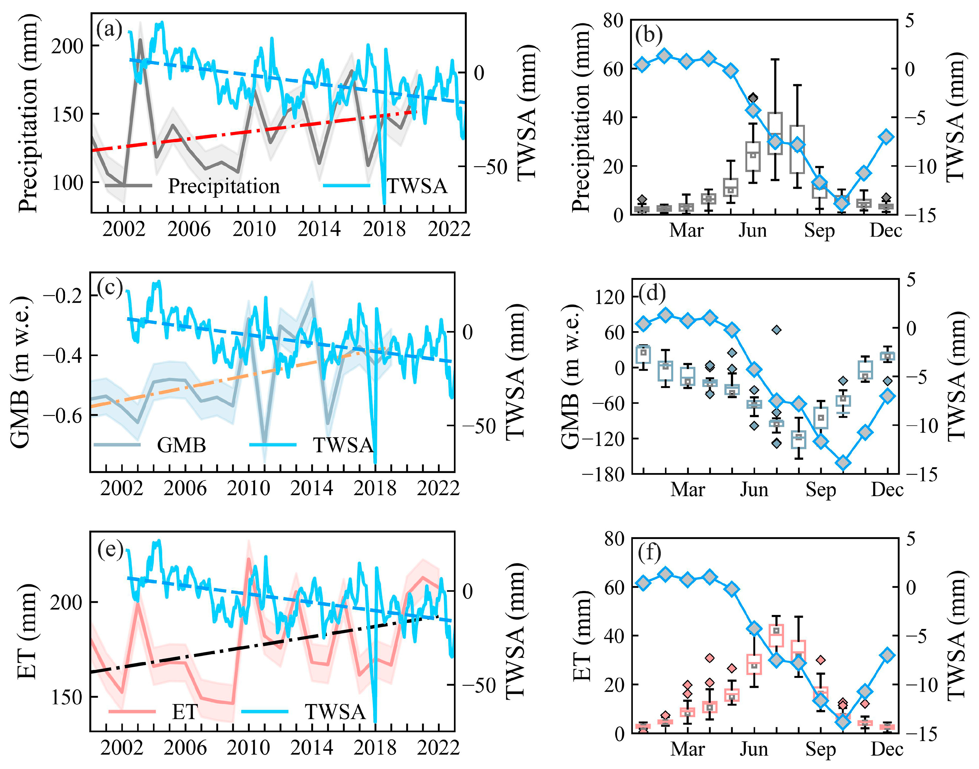
Figure 11.
Comparisons of spatially averaged monthly TWSA derived from GRACE TWS, GLDAS TWS and WGHM in (a) JBNWC and (b) GLDWM. (b) RMSE between GRACE and GLDAS for the period 2002–2023 and subperiods 2002–2010 and 2011–2023. Comparison of TWS trends derived from GRACE (FO), GLDAS, and WGHM in (d) JBNWC and (e) GLDWM. Comparison of water intensity for the period 2000–2010 and 2011–2020 in (f) JBNWC and (g) GLDWM. WI refers to water withdrawal intensity.
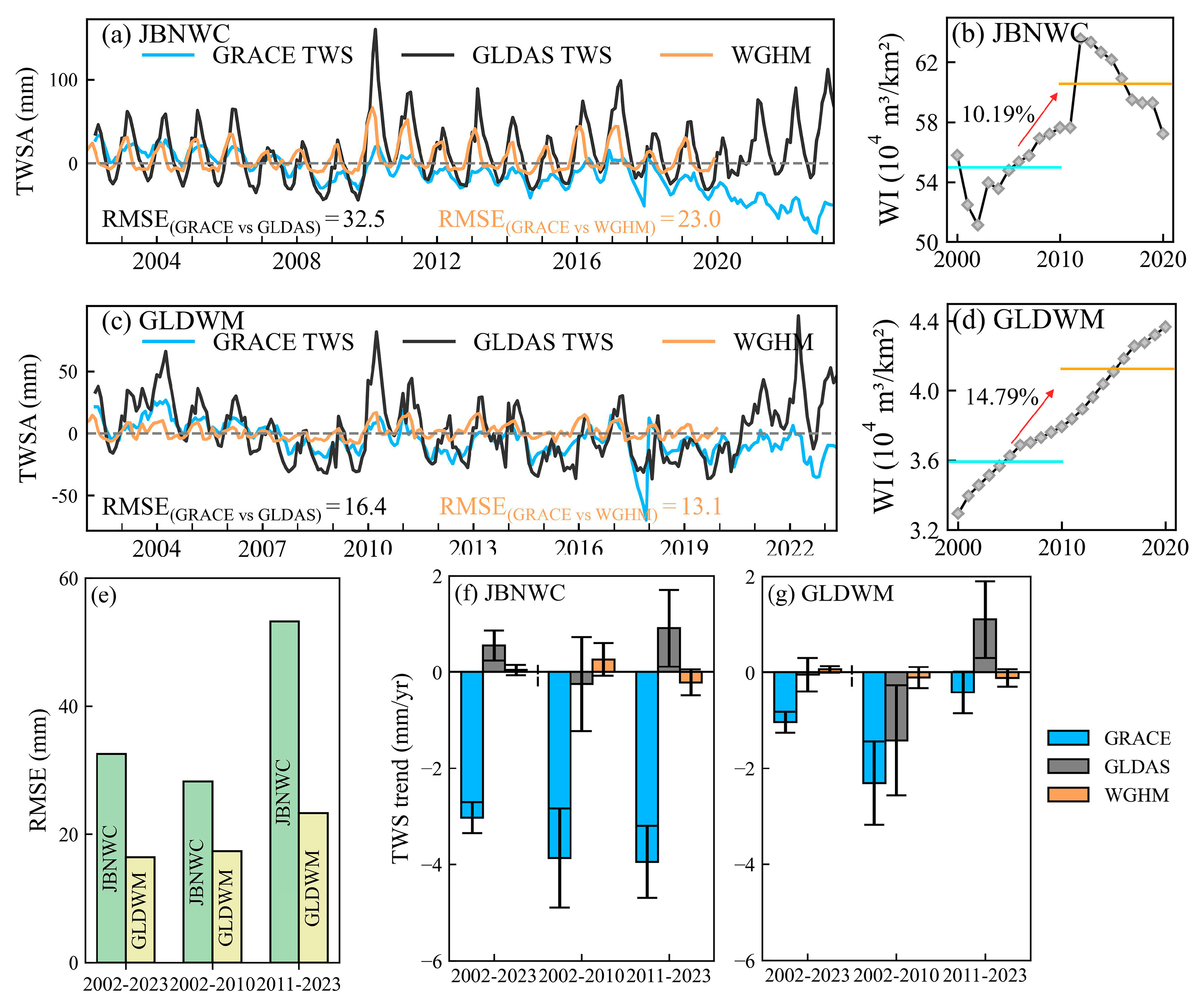

Table 1.
The basic information on the data used in this study.
| Type | Data sources | Temporal resolution |
Spatial resolution |
Date period |
| Precipitation (P) | Meteorological stations CRU v4.05 ERA5-Land GPCC |
Monthly Monthly Monthly Monthly |
Point 0.5° 0.1° 0.25° |
1962–1998 1962–1998 1962–1998 1962–2020 |
| Evapotranspiration (ET) | Noah-LSM ERA5-Land GLEAM 3.5a |
Monthly Monthly Monthly |
0.25° 0.1° 0.25° |
1998–2023 1998–2023 1998–2023 |
| Temperature (T) | Meteorological Stations CRU v4.05 ERA5-Land |
Monthly Monthly Monthly |
Point 0.5° 0.1° |
1962–1998 1962–1998 1962–2023 |
| Land surface temperature (LST) | ERA5-Land | Monthly | 0.1° | 2002–2023 |
| Potential evapotranspiration (PET) | ERA5-Land | Monthly | 0.1° | 2002–2023 |
| Leaf area index (LAI) | ERA5-Land | Monthly | 0.1° | 2002–2023 |
| Normalized difference vegetation index (NDVI) | MOD13C2v061 | Monthly | 0.05° | 2002–2023 |
| Digital elevation model (DEM) | SRTM 90m DEM V4.1 | – | 90m | – |
| Soil texture variables | HWSD2 | – | 1:1,000,000 | – |
| Runoff, Surface runoff (SurR), Subsurface runoff (SubR) | ERA5-Land | Monthly | 0.1° | 2002–2023 |
| Soil moisture (SM) | ERA5-Land | Monthly | 0.1° | 2002–2023 |
| Snow water equivalent (SWE) | ERA5-Land | Monthly | 0.1° | 2002–2023 |
| GRACE and GRACE-FO | CSR-M RL06 JPL-M RL06 GSFC-M RL06 |
Monthly Monthly Monthly |
0.25° 0.5° 0.5° |
2002–2023* 2002–2023* 2002–2023* |
| GLDAS LSMs | CLSM-F2.5 (OL) CLSM-F2.5 (DA) Noah VIC |
Monthly Daily Monthly Monthly |
1.0° 0.25° 0.25° 1° |
2002–2023 2002–2023 2002–2023 2002–2023 |
| GHMs | WaterGAP v2.2d | Monthly | 0.25° | 2001–2016 |
| Water withdrawal intensity (WI) | widyear_1km | Annual | 1km | 2002–2020 |
| Population | Statistical Yearbook | Annual | – | 2000–2023 |
| Sown area | Statistical Yearbook | Annual | – | 2000–2023 |
| livestock | Statistical Yearbook | Annual | – | 2000–2023 |
| GDP | Statistical Yearbook | Annual | – | 2000–2023 |
Note: GRACE, gravity recovery and climate experiment; GRACE-FO, GRACE follows-on; * represents the data gaps between GRACE and GRACE-FO. GLDAS, the global land data assimilation system. LSM, the land surface model. OL, open loop. DA, data assimilation. GHMs, global hydrological models.
Table 2.
Interannual trends in GWSA in different basins before and after removal of glaciers (cm/a).
Table 2.
Interannual trends in GWSA in different basins before and after removal of glaciers (cm/a).
| Basins name | Before (mm/yr) | After (mm/yr) |
|---|---|---|
| NTRB | -4.04 | -3.96 |
| IRB | -0.72 | -0.96 |
| URB | -1.12 | -1.14 |
| ERB | -2.77 | -2.77 |
| Gurbantunggut | -2.63 | -2.63 |
| KRB | -0.27 | -0.33 |
| BRB | -0.31 | -0.33 |
| ZRB | -0.80 | -0.84 |
| ULB | -0.82 | -0.82 |
Disclaimer/Publisher’s Note: The statements, opinions and data contained in all publications are solely those of the individual author(s) and contributor(s) and not of MDPI and/or the editor(s). MDPI and/or the editor(s) disclaim responsibility for any injury to people or property resulting from any ideas, methods, instructions or products referred to in the content. |
© 2025 by the authors. Licensee MDPI, Basel, Switzerland. This article is an open access article distributed under the terms and conditions of the Creative Commons Attribution (CC BY) license (http://creativecommons.org/licenses/by/4.0/).
Copyright: This open access article is published under a Creative Commons CC BY 4.0 license, which permit the free download, distribution, and reuse, provided that the author and preprint are cited in any reuse.


