
Submitted:
27 March 2025
Posted:
29 March 2025
You are already at the latest version
Abstract
The roughness of the Earth’s surface dictates the nature of air flow across it. During some parts of the year, a large portion of the Earth’s surface is snow covered, and the roughness of the snow surface varies over the snow season and over space. Detailed meteorological data that are necessary to access the aerodynamic roughness (z0) are not widely collected and as such the geometry of a surface can be used to estimate z0. Here we present a formulation and the corresponding computer code to compute z0 based on the Lettau (1969) geometric approach. We apply it to three snow surface datasets, each at different phases of the snowpack (and each at two resolutions): fresh snow accumulation (1 m2 at 1 and 10 mm), peak accumulation (1 km2 at 1 and 10 m) and ablation sun cups (25 m2 at 5 and 50 mm). The new code produces a mean z0, as well as a histogram of all z0 values for each individual roughness element (10s of thousand for the 1000 x 1000 grids), as well as directional z0 diagrams, which can be matches with the wind rose for the location. The formulation includes two parameters that may optionally be applied to smooth the surface before calculating z0. By calculating z0 as a function of these two parameters, we demonstrate the sensitivity of the z0 value to these parameter choices.
Keywords:
z0
; Lettau geometry z0
; snow roughness
1. Introduction
Shallow, seasonal snowpack is a critical reservoir for yearly water yield in the western US [1,2]. The snowpack acts as a temporary water storage system and is essential for all regional hydrology, influencing water availability for all natural ecosystems, agricultural, urban systems. Consequently, precise modeling of snowpack dynamics is crucial for accurate estimations of snowmelt [3]. Within hydrologic and cryospheric modeling, the aerodynamic roughness length, , is considered a control on the latent and sensible heat transfer processes due to its reliance on wind speed, direction, and underlying topographic features [4,5,6]. Because of this influence, has a substantial control on snowpack evolution, redistribution, melt rates, and melt water [2,6,7,8].
Additionally, snow is the most reflective naturally occurring surface type on Earth and it covers a significant portion of the globe, including as much as 50% of the land mass of the Northern Hemisphere each season. In its pure state snow reflects as much as 98% of incident solar radiation [9,10]. Rough snow absorbs more solar energy than pure snow, which affects both local melt rates as well as the global climate energy budget [11]. As the snow surface roughness increases, it absorbs more solar energy, increasing the snow melt rate and the amount of energy retained in the thermodynamic system. As such, the snowpack surface plays an important role in the Earth’s total energy budget through reflection and absorption of solar energy [2,12]. Accurately measuring snow surface roughness is essential to understanding this interaction with solar radiation and predicting its effects on snowmelt and climate.
Originally defined for studies of wind profiles, is effectively the height above a surface at which the wind velocity is zero [5,6,13]. Several wind velocities at varying heights are required to quantify using the wind profile method [5,14]. The measured wind velocities are then plotted against the natural log of the height, resulting in the natural log of as the y-intercept of the best linear fit. The magnitude of varies with surface roughness; as surface roughness increases, so does . Fresh snow on a flat, undisturbed surface can have a as low as 0.0002 meters, reflecting its highly smooth and uniform characteristics. In contrast, the surface of a debris-covered glacier presents a heterogeneous texture, leading to values that typically range between 0.005 and 0.5 meters [2,15]. These variations indicate the impact of surface properties on aerodynamic roughness, which directly influences snow processes. Given this wide variability, accurately determining for specific sites is critical to improving the precision of hydrologic and cryospheric models [16,17]. Site-specific values capture variations in land cover, topography, and environmental factors, which generic or averaged estimates cannot adequately represent [17].
Calculating a site-specific value has historically been challenging due to the reliance on a complex, multi-level wind tower to measure the wind profile [2,14]. These traditional methods, while effective, are labor-intensive, spatially limited, and provide sparse data points. However, advancements in remote sensing technologies have significantly improved the feasibility and accuracy of estimating over large surface areas [18]. Remote sensing techniques, particularly LiDAR [19] and more recently photogrammetry [20], can integrate the detailed topographic surface and the snowpack surface properties [17,18]. This geometrically based approach enables the calculation of values across extensive and complex landscapes, providing higher spatial resolution and broader coverage than previously possible. This new methodology of calculation may supplement or replace traditional techniques of determining .
Aerodynamic roughness length is a calculated parameter which characterizes the loss of wind momentum due to surface roughness [6,21]. For this study, the well-known formula developed by Lettau in 1969 [13] is utilized:
where h is the “average vertical extent," or “effective obstacle height,” measured in cm, s is the “silhouette area of the average obstacle,” measured in cm2, and S is the “specific area", or “lot area” measured in cm2 [13]. Figure 1 shows these physical parameters for an idealized case of simple pyramids.
This paper presents code to compute for a surface, provided that the data are on a regular grid. The code can be applied to any surface and at any resolution, and produces the distribution of values with directionality to consider variable wind directions. Wind direction comes into play in the formula (1) in the determination of the silhouette area s. Here, we use three different snow surfaces at different resolutions, as the snow surface, and thus its roughness, can evolve rapidly [8]. We use a fresh snow surface at 1 mm resolution, a snow surface at the time of peak accumulation at 1 m resolution, and a melting snow with sun cups at 5 mm resolution. The three surfaces are initially assessed for an area of 1000 by 1000 pixels and then the resolution is coarsened by an order of magnitude through averaging to a 100 by 100 pixel grid.
2. Methodology
In this section, we describe the method of computing on LiDAR data. This code takes as input elevation data measured on a regular grid along with a vector indicating the direction the wind is blowing. Since the surface is comprised of obstacles that are nonuniform in shape and size, we approach the computation element-wise. That is, we consider each obstacle as an individual roughness element.
To compute we first to segment the surface into roughness elements (the obstacles) , . We then find the lot area , silhouette area , and height of each obstacle. The value of for the surface as given by Equation (1) is the sum:
We detail our approach below.
2.1. Segmentation into Roughness Elements
One of the challenges when computing on real-world data is separating individual roughness elements when such elements are of non-uniform shape and size. We approach this problem using the watershed algorithm [22]. The watershed algorithm segments a topographic relief into catchment basins centered around each local minimum. As roughness elements correspond intuitively to local maxima of the surface, we first invert the surface. For a surface with points , the inverted surface consists of the set of points . Maxima (minima) of the inverted surface correspond to minima (maxima) of the original surface. Hence, the watershed algorithm applied to the inverted surface yields a segmentation into elements associated to each local maximum of the original surface. These segments are our individual roughness elements, or obstacles.
Intuitively, the watershed algorithm places a marker at each local minimum (maximum in the original data), and floods the relief. The level of the flood is the same increases with time at the same rate in all catchment basins. As the level of the flood increases, eventually the floods originating at two distinct catchment basins will meet, at which point a watershed line is added. The process is continued until the entire relief is flooded and therefore segmented. In our case, each watershed segmentation is associated with a single local maximum, and we consider it to be a single roughness element.
2.2. Computing Areas and Heights
The vertical silhouette area of an obstacle represents the area that is upwind, i.e., the silhouette of the region hit directly by the blowing wind. First, we compute the surface normal vector for every data point using a standard bicubic interpolation in all 3 directions. This takes into account not just immediate neighbors, but nearby data points as well. Projecting each normal vector onto the wind direction vector and retaining only the points that result in a nonzero negative projection indicates data points on the surface that will be hit directly by the wind.
In a single watershed element, we identify all data points which comprise the region hit by the wind and will use them to determine the vertical silhouette area of the obstacle. For each data point determined to be in the upwind region, a general unit square the extent of a pixel is transformed using Rodrigues’ formula [23], so that the normal vector of the square is aligned with the normal vector associated with the data point. The square is then projected onto the subspace perpendicular to the direction of the wind. The area of the resulting parallelogram is computed and contributes to the vertical silhouette. To compute the vertical extent, we again restrict to the data points associated to upwind regions and subtract the minimum height from the maximum height. The lot area is the area of the roughness element, which is easily scaled from the number of points segmented into each watershed.
Using the above quantities, a value for is computed for each roughness element and averaged over the entire surface. Since there are thousands to tens of thousands of roughness elements per million pixels, the output is also histogram of values. Further, while the wind direction tends to be consistent, especially over a snow surface [24], the computation can performed directionally.
2.3. Smoothing of the Surface
Two optional modifications may be applied to the data before separating individual roughness features of the surface via the watershed algorithm. An optional Gaussian filter may be applied to the surface (in our code) that smoothens the surface so that there are fewer roughness features associated with small watershed regions. This may help, for instance, in removing small roughness features coming from measurement errors of the surface. This filter smooths by taking a weighted average of neighboring points, where the weight is determined by a symmetric two-dimensional Gaussian (with standard deviation ) centered at each point. This dampens or removes high frequency features, i.e., small perturbations, and acts as a low-pass filter. This is a common filter choice for smoothing topographical data ([25,26,27,28]) and is included as an optional filter in some GIS software ([29,30]). The symmetric 2-D Gaussian smoothing kernel with standard deviation is given as
where the size of the filter is given by . Additionally, maxima less than a specified percentage higher than the surrounding area may be suppressed resulting in fewer maxima and a simplified watershed profile. This is a common technique in image analysis to reduce over-segmentation ([31]).
3. Datasets and Preparation
3.1. Snow Surface Datasets
The value was computed for three resolutions of data representing different time periods of the snowpack evolution (accumulation, peak, and ablation) (Table 1 and Figure 2). The fresh snow (FS-FC) dataset was collected during a new snowfall event with snow snowcover existing on the ground. The FS-FC raw point cloud was at a resolution finer than 1 mm. The ablation-sun cup (SC-PH) dataset were collected when substantial sun cups were present during snowmelt. The SC-PH raw point cloud was at a resolution of about 3 mm. Both datasets were collected with a Faro Focus3D X 130 model Terrestrial lidar Scanner (TLS) (https://www.faro.com/). The ablation-sun cup data were collected as three separate scans due to the nature of the surface, i.e., sun cups. The three point cloud were sewn together with Cloud Compare, an open-source software for 3D point cloud and mesh analysis ([32]; https://www.danielgm.net/cc/).
The peak accumulation (PA-NS) data were from the Niwot Saddle behind Boulder, Colorado U.S.A., that is part of the Niwot Long Term Ecological Research Program (https://nwt.lternet.edu/). The point clouds were not available publicly, and the data were already interpolated to a 1-m grid. The data were obtained as per Harpold et al. [33]. All data are available online [34].
Figure 2.
The three gridded datasets used in the computation as 1000 by 1000 pixels (a, d, g) and coarsened by a factor of 10 (b, e, h), plus the histograms of the distribution of elevation for each surface (c, f, i) for (a, b, c) fresh snow in Fort Collins (lines in 0.005 m intervals), (d, e, f) peak accumulation at Niwot Saddle (lines in 2 m intervals), and (g, h, i) ablation sun cups in the Poudre Headwaters (lines in 0.05 m intervals). The surfaces have been detrended to remove any slope-based bias [35]. As such, black lines/areas are above the datum of zero while red lines/areas are below the datum of zero.
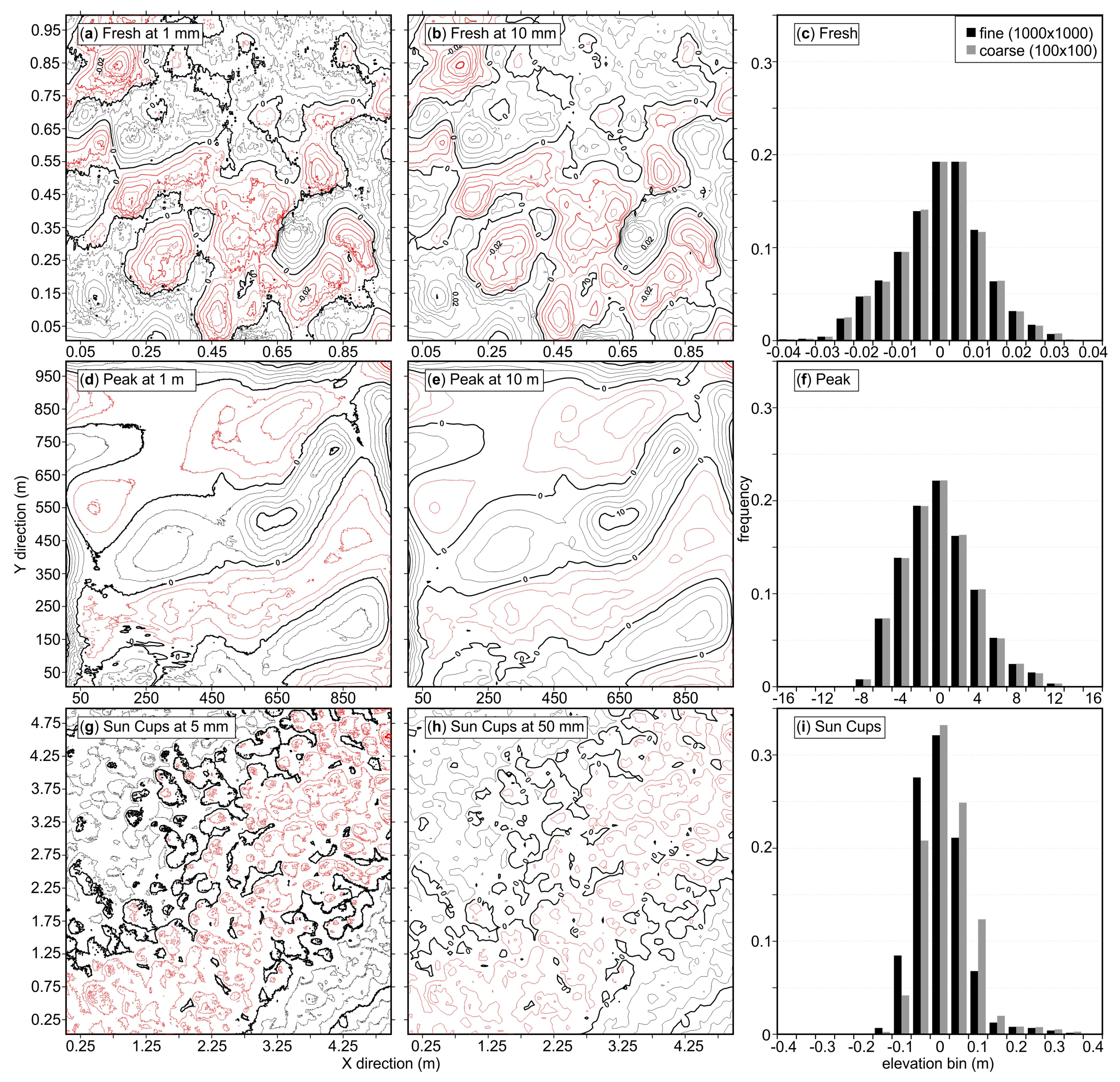
The elevation range is larger for the more coarse surfaces (Figure 2d versus Figure 2g and Figure 2a). However, comparing the elevation range (Figure 2c, f and i) to the resolution illustrates less prominence in roughness features as the resolutions becomes larger. Coarsening the resolution of the individual datasets did not alter the elevation distribution, except for the sun cup surface (Figure 2i). These surfaces present three different snowpack conditions with features highlighted by the varying resolutions.
3.2. Data Preparation
Following the collection of the lidar scans (fresh snow and ablation-sun cup datasets), each raw point cloud (three sewn together for SC-PH) was processed and evaluated using Cloud Compare. The scans were then cropped to the area of interest, ensuring that the dataset was limited to the preferred geographic region or feature under study. Additionally, any rogue points, such as noise or erroneous data points often caused by environmental elements, were identified and removed to enhance the accuracy and clarity of the dataset. The cropped point cloud was imported into Golden Software’s Surfer ([36]; https://www.goldensoftware.com/products/surfer). The software allows the user to interpolate the data using pre-defined methodology, such as kriging, used for this study, and user defined resolutions. The kriging method was chosen because of its capacity to account for the spatial arrangement of measured points, which is relevant to the surface roughness analysis. The result is a smoothed, gridded, surface, instead of the point cloud, which is required to be used within the code.
Each gridded dataset was detrended in the X and Y directions to reduce bias from sloping surfaces [35]. Since the Niwot Saddle covered a hillslope with substantial terrain variation (see [37]), the surface (PA-NS) was detrended three times. First, there was a linear detrend to removed the overall slope. Then, a 3rd-order polynomial was fitted to the surface to remove the saddle feature. Finally, a linear detrend removed the positioning bias.
4. Results
The value of varied as a function of resolution (Table 2). This is both for the resolution of the original data, i.e., fresh snow versus peak accumulation versus ablation sun cups, and coarsening of the data. There are fewer elements as we coarsen the data, and thus, fewer elements become more granular. For the finest resolution surface (fresh snow), the elements are the smallest.
Most of the roughness elements were small and thus had a low value (a left skew in Figure 3). For the finer resolution grids (Figure 3a, c, and e), more than 80% of the value were in the lowest bin. The sun cup surface had the most undulations (Figure 2) c and d), and the most elements at the original and coarsened resolution (Table 2). At smaller scales, there are many more features with a low value.
The code computes with directionality, which does vary as a function of coarsening (Figure 4). The smoothest (lowest values) are not the same direction between the original and coarsened datasets. This is relevant because, while wind tends to blow consistently from the same direction due to terrain influences [38], it does vary [39].
As discussed in Section 2.3, two optional parameters, and % of maximum height, may be chosen to smoothen the surface before calculating . For the values reported in Table 2 and Figure 3 and Figure 4, no smoothing was implemented (both smoothing parameters were set to 0). To illustrate how depends on these parameters, we calculated for ranges parameter values for the Niwot 1 m data set. Figure 5 shows the results. For small values of , is insensitive to the choice of , as seen in the left panel of Figure 5. For larger values of , the surface is smoothed to the extent that essential roughness features are lost. Figure 6 illustrates how the watersheds associated with peaks of the surface decrease as increases. However, does depend more sensitively to the % parameter for small values of , as seen in the right panel of Figure 5.
5. Discussion
Lettau’s formulation [13] of the aerodynamic roughness length , implemented in this paper, is a geometric representation of the surface. There are other formulations [40,41], but they do not appear to be as useful for snow [18]. Lettau’s formulation [13] is widely used for snow and glacier surfaces [2,14,42]. With the propensity of spatial surface measurement approaches and data, especially for the snowpack [20,33,43,44,45], the geometric estimation of is a useful approach. As such, this paper provides the computer code to estimate Lettau’s [13] formulation.
Andreas [46] derived an empirical formulation of for sea ice based on the physical roughness of the surface. It used transect data, based on the dominant wind direction, to compute the roughness. The Andreas [46] approach could be applied to spatial datasets to consider changes in wind direction( Figure 4). Wind directions can vary seasonally and even daily based on weather [39].
Following common approaches in image analysis to reduce effects of measurement noise or oversegmentation, the code includes two optional parameters that smoothen the surface before calculating . The first parameter is the standard deviation of the smoothing filter. The second parameter is the % of the maximum height of the surface; peaks with height lower than this percentage height are not included as obstacles contributing to the calculation. We showed the choice of these parameter values does significantly affect the calculated value of . However, in the case of the Niwot 1 m data set, is insensitive to the choice for small values of . The values of these smoothing parameters should be reported in any calculation of using the Lettau method as implemented in this paper. Further work should elucidate how to choose these parameter values to best match an application, such as using the aerodynamic roughness in a simulation of fluid flow across a surface.
Author Contributions
Conceptualization, R.P., S.R.F., I.O., R.A.N., P.D.S. and J.E.S.; methodology, R.P., R.A.N., P.D.S., S.R.F., and J.E.S.; software, R.P., R.A.N., P.D.S., and J.E.S.; validation, R.A.N., P.D.S., J.E.S. and S.R.F.; formal analysis, R.A.N., P.D.S., J.E.S. and S.R.F.; data curation, S.R.F. and J.E.S.; writing—original draft preparation, R.P., S.R.F., J.E.S., R.A.N., and P.D.S.; writing—review and editing, S.R.F., R.A.N., P.D.S. and J.E.S.; visualization, R.A.N., P.D.S., S.R.F. and R.P.; supervision, S.R.F., P.D.S. and I.O.; project administration, S.R.F., I.O., and P.D.S.; funding acquisition, I.O., S.R.F., and P.D.S. All authors have read and agreed to the published version of the manuscript.
Funding
This research was indirectly funded by the U.S. Geological Survey National Institutes for Water Resources (U.S. Department of the Interior), grant number 2019COSANOW, project “The Dynamic Nature of Snow Surface Roughness”, through the Colorado Water Center and at Colorado State University by the National Science Foundation grant number DMS-1615909. The Sun Cup dataset was collected as part of the National Park Service Water Resources Division (NPS-WRD) Task agreement number P16AC00826.
Data Availability Statement
The Peak Accumulation snow surface from Niwot Saddle is available from the Niwot Long Term Ecological Research Program (https://nwt.lternet.edu/), and were identified in Harpold et al. [33]. The Fresh Snow, Peak Accumulation, and Sun Cups snow surfaces are available through Dyrad [34] (https://doi.org/10.5061/dryad.qv9s4mwr2). The code presented in this paper is available at [47].
Acknowledgments
Graham Sexstone of the U.S. Geological Survey acquired the Niwot Sadddle dataset for this work.
Conflicts of Interest
The authors declare no conflicts of interest.
Abbreviations
The following abbreviations are used in this manuscript:
| AOI is the area of interest |
| h is the average vertical extent or effective obstacle height, measured in cm |
| s is the silhouette area of the average obstacle, measured in cm2 |
| S is the specific area or lot area, measured in cm2 |
| is the (geometric) aerodynamic roughness length, measured in m |
References
- Mialon, A.; Fily, M.; Royer, A. Seasonal snow cover extent from microwave remote sensing data: Comparison with existing ground and satellite based measurements. EARSeL eProceedings 1994, 4, 215–225. [Google Scholar]
- Musselman, K.N. , Clark, M.P., Liu, C., Ikeda, C., Rasmussen, R. Slower snowmelt in a warmer world. Nature Climate Change 2017, 7, 214–220. [Google Scholar] [CrossRef]
- Miles, E.S. , Steiner, J.F., Brun, F. Highly variable aerodynamic roughness length for a hummocky debris-covered glacier. Journal of Geophysical Research: Atmospheres 2017, 122, 8447–8466. [Google Scholar] [CrossRef]
- Andreas, E. Parameterizing scalar transfer over snow and ice: a review. Journal of Hydrometeorology 2002, 3(4), 417–432. [Google Scholar] [CrossRef]
- Gromke, C.; Manes, C.; Walter, B.; Lehning, M.; Guala, M. Aerodynamic roughness length of fresh snow. Boundary-Layer Meteorology 2011, 141 (1), 21–34. [CrossRef]
- Smith, M.W. Roughness in the earth sciences. Earth Science Reviews 2014, 136, 202–225. [Google Scholar] [CrossRef]
- Andreas, E. L. A theory for the scalar roughness and the scalar transfer coefficients over snow and sea ice. Boundary-Layer Meteorology 1987, 38 (1–2), 159–184. [CrossRef]
- Fassnacht, S. R.; Williams, M. W.; Corrao, M. V. Changes in the surface roughness of snow from millimetre to metre scales. Ecological Complexity 2009, 6(3), 221–229. [Google Scholar] [CrossRef]
- Kukko, A.; Anttila, K.; Manninen, T.; Kaasalainen, S.; Kaartinen, H. Snow surface roughness from mobile laser scanning data. Cold Regions Science and Technology 2013, 96, 23–35. [Google Scholar] [CrossRef]
- Zhuravleva, T.B. , Kokhanovsky, A. Influence of surface roughness on the reflective properties of snow. Journal of Quantitative Spectroscopy and Radiative Transfer 2011, 112(8), 1352–1368. [Google Scholar] [CrossRef]
- Amory, C.; Naaim-Bouvet, F.; Gallee, H.; Vignon, E. Brief communication: Two well-marked cases of aerodynamic adjustment of sastrugi. The Cryosphere 2016, 10. [Google Scholar] [CrossRef]
- Thackeray, C.W., Fletcher, C.G. Snow albedo feedback: Current knowledge, importance, outstanding issues and future directions. Progress in Physical Geography: Earth and Environment 2016, 40 (3). [CrossRef]
- Lettau, H. Note on aerodynamic roughness-parameter estimation on the basis of roughness-element description. Journal of Applied Meteorology 1969, 8, 828–832. [Google Scholar] [CrossRef]
- Munro, D. S. Surface roughness and bulk heat transfer on a glacier: comparison with eddy correlation. Journal of Glaciology 1989, 35(121), 343–348. [Google Scholar] [CrossRef]
- Brock, B.; Willis, I.; Sharp, M. Measurement and parameterization of aerodynamic roughness length variations at Haut Glacier d’Arolla, Switzerland. Journal of Glaciology 2006, 52(177), 281–297. [Google Scholar] [CrossRef]
- Fassnacht, S. R. Temporal changes in small scale snowpack surface roughness length for sublimation estimates in hydrological modelling. Cuadernos De Investigación Geográfica 2010, 36 (1), 43. [CrossRef]
- Sanow, J.E.; Fassnacht, S.R.; Suzuki, K. How does a dynamic surface roughness affect snowpack modelling? Polar Science 2024, 41(1-2). [CrossRef]
- Sanow, J.E. , Fassnacht, S.R., Kamin, D.J., Sexstone, G.A., Bauerle, W.L., Oprea, I. Geometric versus anemometric surface roughness for a shallow accumulating snowpack. Geosciences 2018, 8(12), 463. [Google Scholar] [CrossRef]
- Hood, J.L.; Hayashi, M. Assessing the application of a laser rangefinder for determining snow depth in inaccessible alpine terrain. Hydrology and Earth System Sciences 2010, 14(6), pp.901-910.
- Nolan, M.; Larsen, C.; Sturm, M. Mapping snow depth from manned aircraft on landscape scales at centimeter resolution using structure-from-motion photogrammetry. The Cryosphere 2015, 9(4), pp.1445-1463.
- Jacobson, M.Z. Fundamentals of atmospheric modeling., 2nd ed.; Cambridge University Press: Cambridge, Great Britain, 2005. [Google Scholar]
- Meyer, F. Topographic distance and watershed lines. Signal processing 1994, 38(1), 113–125. [Google Scholar] [CrossRef]
- Encyclopedia of Mathematics: Rodrigues formula. Available online: https://encyclopediaofmath.org/wiki/Rodrigues formula (accessed on 30 December, 2024).
- Winstral, A.; Elder, K.; Davis, R. E. Spatial snow modeling of wind-redistributed snow using terrain-based parameters. Journal of Hydrometeorology 2002, 3(5), 524–538. [Google Scholar] [CrossRef]
- Lindsay, J.B. Whitebox GAT: A case study in geomorphometric analysis. Computers & Geosciences, 2016 95, 75-84. [CrossRef]
- Lindsay, J. B.; Francioni, A.; Cockburn, J. M. H. LiDAR DEM Smoothing and the Preservation of Drainage Features. Remote Sensing 2016, 11(16), 1926. [Google Scholar] [CrossRef]
- O’Neil, G. L., Saby, L., Band, L. E., & Goodall, J. L. Effects of LiDAR DEM smoothing and conditioning techniques on a topography-based wetland identification model. Water Resources Research,2019, 55(5), 4343-4363.
- Erdbrügger, J., van Meerveld, I., Bishop, K.,Seibert, J. Effect of DEM-smoothing and-aggregation on topographically-based flow directions and catchment boundaries. Journal of Hydrology, 2021, 602, 126717.
- Whitebox Tools. Available online: https://www.whiteboxgeo.com/.
- Conrad, O., Bechtel, B., Bock, M., Dietrich, H., Fischer, E., Gerlitz, L., Wehberg, J., Wichmann, V., and Böhner, J.: System for Automated Geoscientific Analyses (SAGA) v. 2.1.4, Geosci. Model Dev., 2015 8, 1991-2007. [CrossRef]
- The MathWorks, Inc. Imhin Documentation. mathworks.com. Accessed: October 5, 2024. Available online: https://www.mathworks.com/help/images/ref/imhmin.html.
- CloudCompare. Available online: https://www.danielgm.net/cc/ (accessed on 30 December, 2024).
- Harpold, A. A.; et al. LiDAR-derived snowpack data sets from mixed conifer forests across the Western United States. Water Resour. Res. 2024, 50, 2749–2755. [Google Scholar] [CrossRef]
- Fassnacht, S.R.; Sanow, J.E. Fresh Snow and Ablation-Sun Cup Snow Surface Datasets for Evaluation of Geometry Aerodynamic Roughness Code [Dataset]. Dryad 2025. [CrossRef]
- Fassnacht, S. R.; Stednick, J. D.; Deems, J. S.; Corrao, M. V. Metrics for assessing snow surface roughness from digital imagery. Water Resources Research 2009, 45, W00D31. [Google Scholar] [CrossRef]
- Golden Software – Surfer. Available online: https://www.goldensoftware.com/products/surfer/ (accessed on 30 December, 2024).
- Sexstone, G. A.; Fassnacht, S. R.; López-Moreno, J. I.; Hiemstra, C. A. Subgrid snow depth coefficient of variation spanning alpine to sub-alpine mountainous terrain. Cuadernos de Investigación Geográfica/Geographical Research Letters 2022, 48(1), 79-96. [CrossRef]
- Winstral, A; Marks D. Simulating wind fields and snow redistribution using terrain-based parameters to model snow accumulation and melt over a semi-arid mountain catchment. Hydrological Processes 2002, 16(18), 3585-603. [CrossRef]
- Moron, V.; Robertson, A.W.; Qian, J.-H.; Ghil, M. (2015). Weather types across the Maritime Continent: from the diurnal cycle to interannual variations. Front. Environ. Sci. 2015, 2, 65 [. [Google Scholar] [CrossRef]
- Counihan, J. Wind tunnel determination of the roughness length as a function of the fetch and the roughness density of three-dimensional roughness elements. Atmos. Environ. 1971, 5, 637–642. [Google Scholar] [CrossRef]
- Macdonald, R.W.; Griffiths, R.F.; Hall, D.J. An improved method for the estimation of surface roughness of obstacle arrays. Atmos. Environ. 1998, 32, 1857–1864. [Google Scholar] [CrossRef]
- Nield, J.M.; King, J.; Wiggs, G.F.; Leyland, J.; Bryant, R.G.; Chiverrell, R.C.; Darby, S.E.; Eckardt, F.D.; Thomas, D.S.; Vircavs, L.H.; Washington, R. Estimating aerodynamic roughness over complex surface terrain. Journal of Geophysical Research: Atmospheres 2013, 118(23), pp.12-948. [CrossRef]
- Revuelto, J.; López-Moreno, J.I.; Azorín-Molina, C.; Zabalza, J.; Arguedas, G.; Vicente-Serrano, S.M. Mapping the annual evolution of snow depth in a small catchment in the Pyrenees using the long-range terrestrial laser scanning. Journal of Maps 2014, 10(3), pp.379-393. [CrossRef]
- Nolan, M.; Larsen, C.; Sturm, M. Mapping snow depth from manned aircraft on landscape scales at centimeter resolution using structure-from-motion photogrammetry. The Cryosphere 2015, 9, 1445–1463. [Google Scholar] [CrossRef]
- Revuelto, J.; Alonso-Gonzalez, E.; Vidaller-Gayan, I.; Lacroix, E.; Izagirre, E.; Rodríguez-López, G.; López-Moreno, J.I. Intercomparison of UAV platforms for mapping snow depth distribution in complex alpine terrain. Cold Regions Science and Technology 2021, 190, p103344. [Google Scholar] [CrossRef]
- Andreas, E.L. A relationship between the aerodynamic and physical roughness of winter sea ice. Q. J. R. Meteorol. Soc. 2011, 137, 1581–1588. [Google Scholar] [CrossRef]
- z0 Lettau LiDAR Watershed Code. [GitHub Repository] Available online: https://github.com/rneville/Z0-Lettau-LiDAR-Watershed 2025.
Figure 1.
Physical parameters used in Lettau’s formula given by Equation (1). AOI is the Area Of Interest.
Figure 1.
Physical parameters used in Lettau’s formula given by Equation (1). AOI is the Area Of Interest.
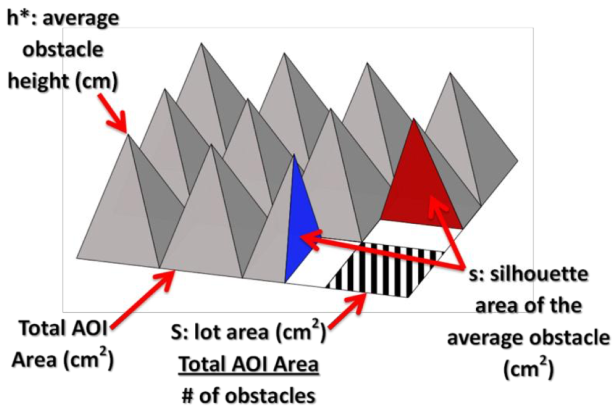
Figure 3.
Histogram of values for the peak accumulation on fresh snow in Fort collins at (a) 0.001 m and (b) 0.01 m resolutions, the Niwot Saddle (c) at 1 m and (d) 10 m resolutions, and the ablation sun cups at the Poudre Headwaters at (e) 0.005 m and (f) 0.05 m resolutions for an eastward wind.
Figure 3.
Histogram of values for the peak accumulation on fresh snow in Fort collins at (a) 0.001 m and (b) 0.01 m resolutions, the Niwot Saddle (c) at 1 m and (d) 10 m resolutions, and the ablation sun cups at the Poudre Headwaters at (e) 0.005 m and (f) 0.05 m resolutions for an eastward wind.
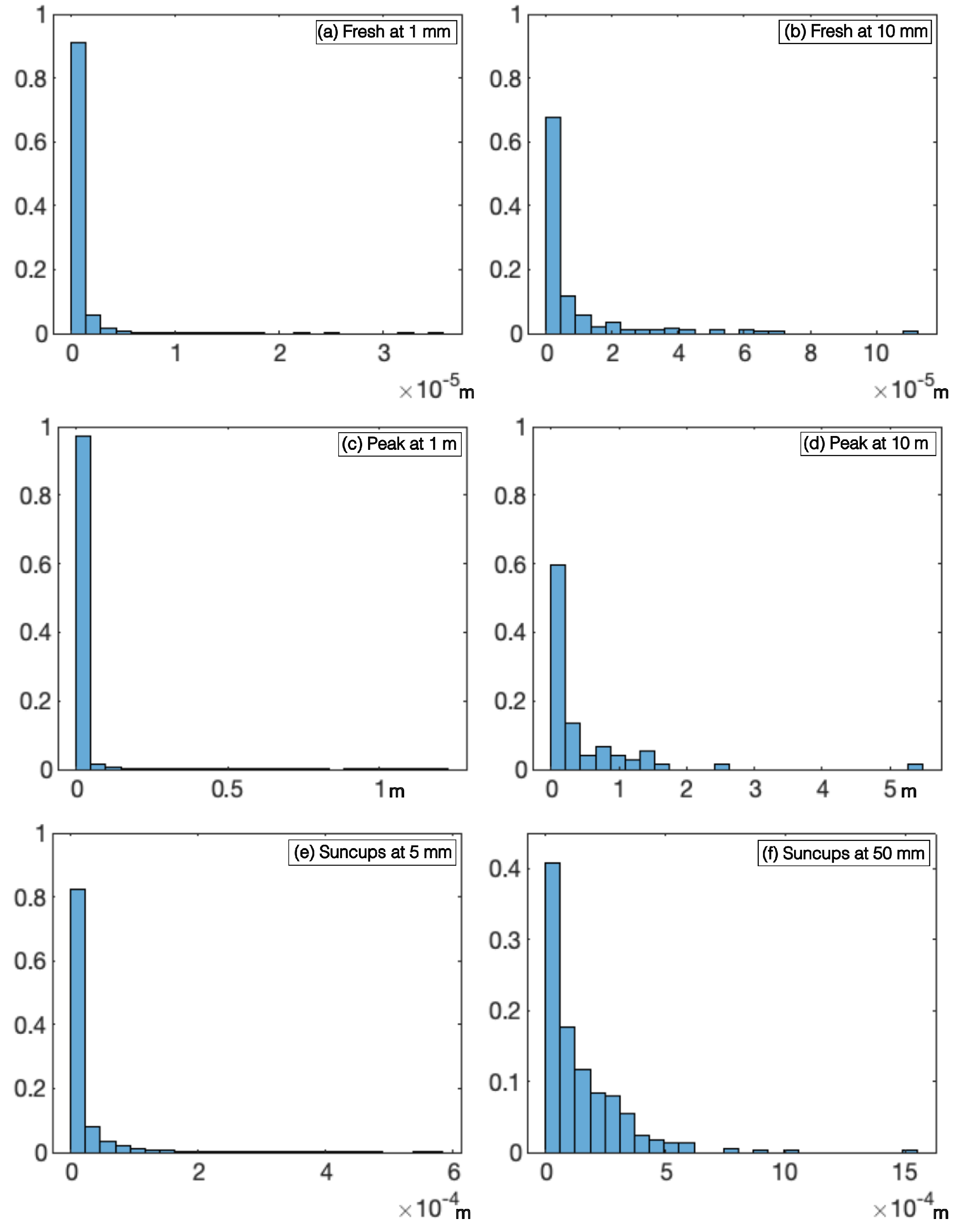
Figure 4.
The mean value varies with the direction from which the wind hits the surface. Shown above is the mean as it varies with wind direction from 24 different directions for the peak accumulation on fresh snow in Fort Collins at (a) 0.001 m and (b) 0.01 m resolutions, the Niwot Saddle (c) at 1m and (d) 10 m resolutions, the ablation sun cups at the Poudre Headwaters at (e) 0.005 m and (f) 0.05 m resolutions.
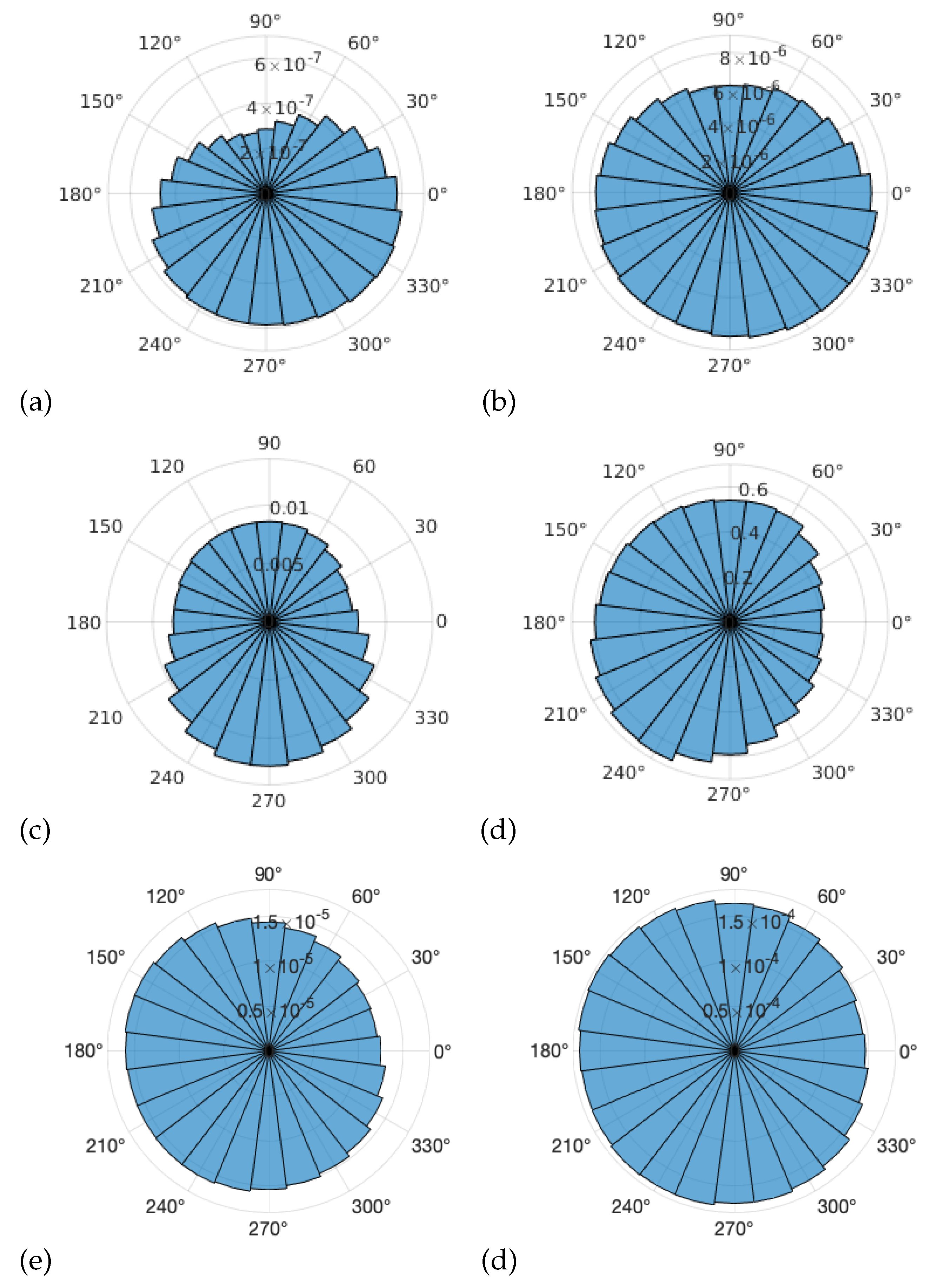
Figure 5.
Shown is the sensitivity of the mean of the Niwot Saddle at 1m resolutions for an eastward wind to changes in the parameter (left) in the Gaussian smoothing and to changes in both the % peak suppression parameter and to (right) in the preliminary filtering step.
Figure 5.
Shown is the sensitivity of the mean of the Niwot Saddle at 1m resolutions for an eastward wind to changes in the parameter (left) in the Gaussian smoothing and to changes in both the % peak suppression parameter and to (right) in the preliminary filtering step.
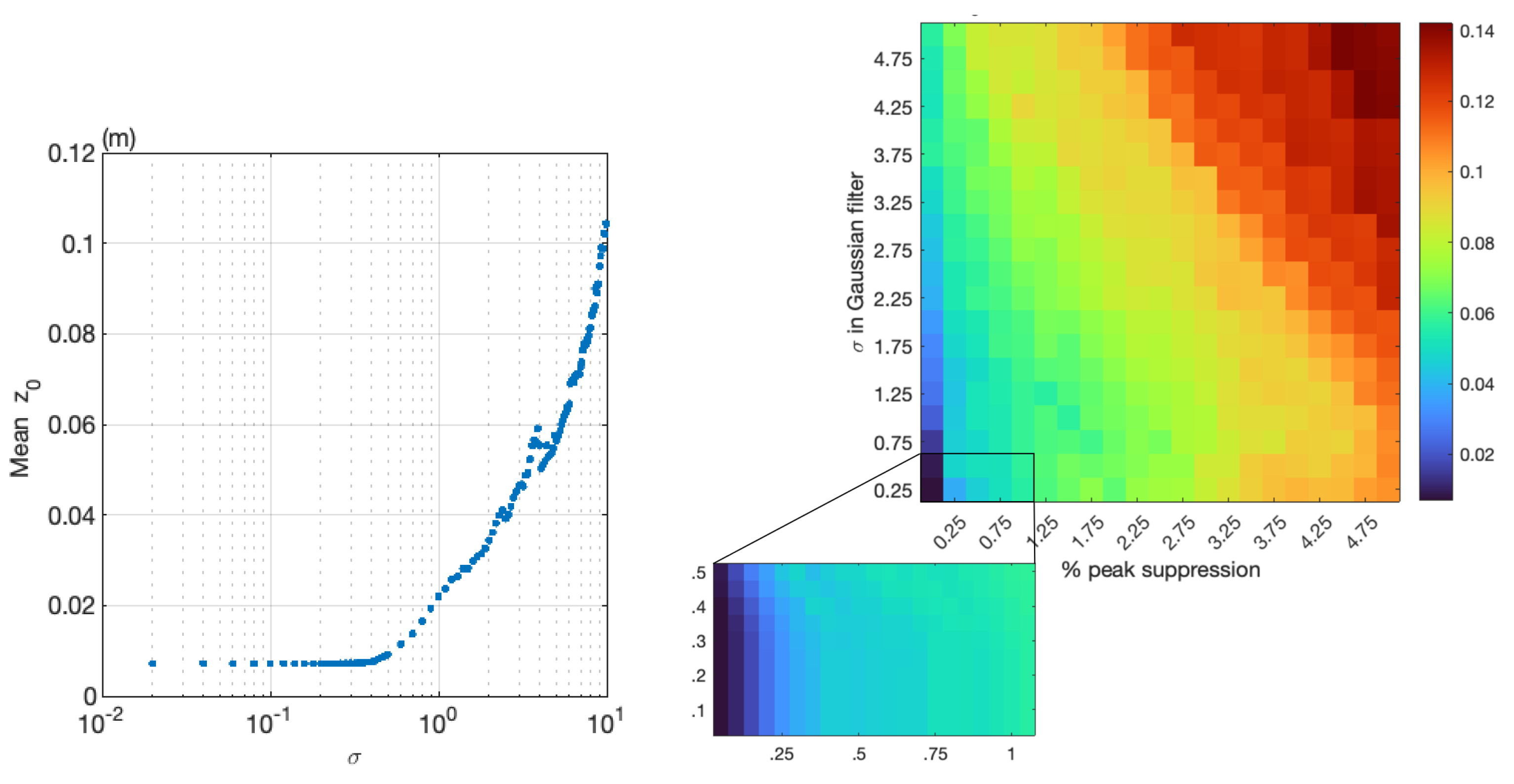
Figure 6.
The watershed of a small subset of the Niwot Saddle at 1m resolution for the (a) raw data and data filtered via Gaussian smoothing with (b) , (c), and (d).
Figure 6.
The watershed of a small subset of the Niwot Saddle at 1m resolution for the (a) raw data and data filtered via Gaussian smoothing with (b) , (c), and (d).
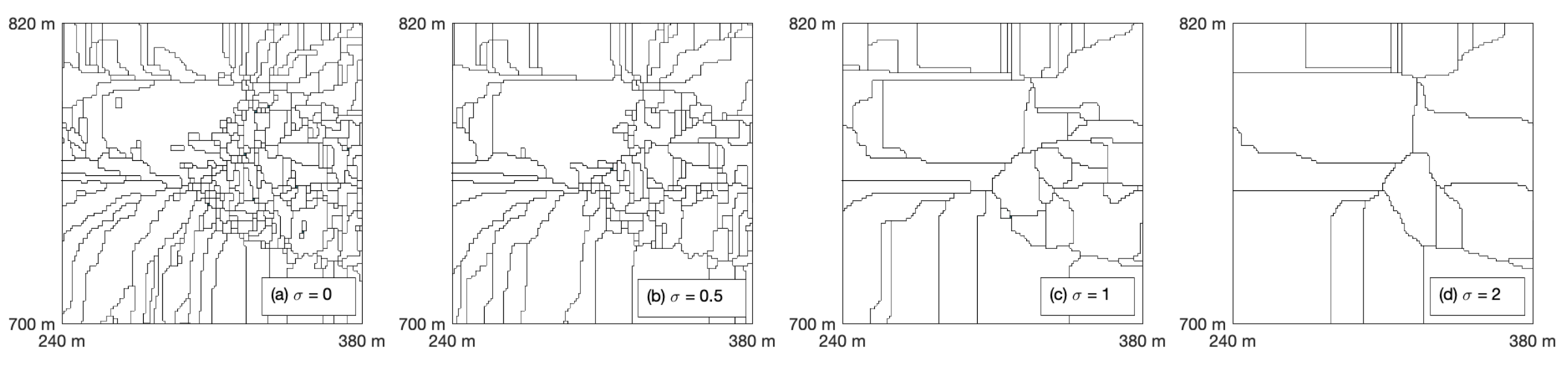

Table 1.
Summary of the three datasets used in the computation. All are for a 1000 by 1000 pixel area at the stated resolution. Data were obtained in the state of Colorado, U.S.A.
Table 1.
Summary of the three datasets used in the computation. All are for a 1000 by 1000 pixel area at the stated resolution. Data were obtained in the state of Colorado, U.S.A.
| dataset | fresh snow | peak accumulation | ablation - sun cups |
|---|---|---|---|
| short name/code | FS-FC | PA-NS | SC-PH |
| location | Fort Collins | Niwot Saddle | Poudre headwaters |
| latitude, longitude | 40.6, -105.1 | 40.0547, -105.5890 | 40.4396, -105.7739 |
| date acquired | 19 April 2021 | 20 May 2010 | 13 June 2017 |
| resolution (m) | 0.001 | 1 | 0.05 |
Table 2.
Number of elements identified for each datasets and resolution with the mean value (in cm) for wind blowing from west to east.
Table 2.
Number of elements identified for each datasets and resolution with the mean value (in cm) for wind blowing from west to east.
| surface | fresh snow | - | peak accumulation | - | ablation - sun cups | - |
|---|---|---|---|---|---|---|
| resolution (m) | 0.001 | 0.010 | 1 | 10 | 0.005 | 0.050 |
| elements | 7366 | 195 | 21090 | 74 | 36259 | 380 |
| mean (x) | 0.00054 | 0.0075 | 9.4 | 421 | 0.012 | 0.14 |
Disclaimer/Publisher’s Note: The statements, opinions and data contained in all publications are solely those of the individual author(s) and contributor(s) and not of MDPI and/or the editor(s). MDPI and/or the editor(s) disclaim responsibility for any injury to people or property resulting from any ideas, methods, instructions or products referred to in the content. |
© 2025 by the authors. Licensee MDPI, Basel, Switzerland. This article is an open access article distributed under the terms and conditions of the Creative Commons Attribution (CC BY) license (http://creativecommons.org/licenses/by/4.0/).
Copyright: This open access article is published under a Creative Commons CC BY 4.0 license, which permit the free download, distribution, and reuse, provided that the author and preprint are cited in any reuse.


