
Submitted:
20 March 2025
Posted:
27 March 2025
You are already at the latest version
Abstract
The increase in malicious cyber activities has generated the need to produce effective tools for the field of digital forensics and incident response. Artificial intelligence (AI) and its fields, specifi- cally machine learning (ML) and deep learning (DL), have shown great potential to aid the task of processing and analyzing large amounts of information. However, models generated by DL are often considered “black boxes”, a name derived due to the difficulties faced by users when trying to understand the decision-making process for obtaining results. This research seeks to address the challenges of transparency, explainability and reliability posed by black box models in digital forensics. To do this, explainable artificial intelligence (XAI) is explored as a solution. This approach seeks to make DL models more interpretable and understandable by humans. The SHAP (SHapley Additive eXplanations) and LIME (Local Interpretable Model-agnostic Explanations) methods will be implemented and evaluated as a model-agnostic technique to explain predictions of the generated models for forensic analysis. In order to make transparent the decision-making process in the models, and to evaluate the confidence of the generated results
Keywords:
Forensic Analysis
; XAI
; UNSW-NB15
; SHAP
; LIME
; XGBoost
; TabNet
1. Introduction
The rapid digitalization of society has led to an unprecedented surge in cybercriminal activities, with an increasing number of connected devices and users becoming potential targets [1,2]. These cyber threats encompass various malicious objectives, including unauthorized data collection from individuals and organizations, ransomware attacks on devices containing confidential information, and illicit content trading in dark markets [3].
Digital forensics, a branch of forensic science, focuses on the recovery, preservation, and analysis of electronic data crucial for criminal investigations. This field encompasses the examination of computers, hard drives, mobile devices, and other data storage media [4,5]. The convergence of escalating cyber attacks and the growing diversity of vulnerable devices has necessitated the adaptation of forensic analysis and incident response methodologies, particularly through the integration of artificial intelligence (AI) technologies [6].
AI, specifically machine learning (ML) algorithms, has demonstrated significant potential in forensic triage by enabling analysts to classify and categorize vast amounts of data while automating repetitive tasks [7]. However, this technological advancement presents unique challenges in the context of digital forensics, where practitioners are bound by strict ethical codes and legal requirements. These protocols ensure that forensic analysis is conducted fairly, objectively, and transparently while adhering to established legislation [8,9].
A critical challenge emerges from the opacity of AI systems, particularly those based on deep neural networks (DNNs). This opacity, known as the "black box problem" [10,11], creates difficulties in interpreting and explaining the logic behind AI-generated conclusions. This limitation has significant implications for the legal admissibility of evidence and the overall integrity of forensic investigations [12].
Explainable Artificial Intelligence (XAI) has emerged as a promising approach to address these challenges. XAI is a subfield of artificial intelligence focused on making ML models more interpretable and explainable to humans. It encompasses processes and methods that enable human users to understand and trust the outputs generated by ML algorithms [13,14,15]. XAI techniques achieve this by unveiling the decision-making process, identifying potential biases, debugging and improving models, and enhancing trust and transparency [16]. Interpretability, a closely related concept, is described as the degree to which a human can understand the cause of a decision [17,18]. It has also been defined as the ability to explain or present results in understandable terms for a human [19] or as methods and models that make the behavior and predictions of ML systems comprehensible to humans [20].
XAI techniques can be categorized into local and global explainers. Local explainers focus on elucidating the reasoning behind the model’s predictions for individual data points, analyzing how the model arrives at specific predictions based on its decision history. In contrast, global explainers aim to understand the overall behavior of the model across the entire dataset, identifying patterns in the model’s outputs and determining which input variables have the most significant influence on predictions [21].
This research aims to evaluate XAI approaches and techniques within the digital forensics context, addressing challenges related to transparency, explicability, and reliability of deep learning models. We focus on examining implementation and design methods to ensure compliance with ethical and legal requirements in forensic computing [22].
1.1. Research Contribution
This study contributes to the field by:
- Conducting a critical review of XAI techniques in digital forensic applications.
- Examining theoretical principles underlying XAI methods.
- Analyzing current challenges and limitations in digital forensics regarding AI model transparency.
- Implementing and evaluating multiple XAI methods in practical forensic case studies.
- Proposing future research directions for XAI applications in digital forensic.
2. Explainability and Interpretability Methods and Datasets
This section presents LIME (Local Interpretable Model-Agnostic Explanations) and SHAP (SHapley Additive Explanations), two widely used methods for interpreting the behavior of complex models, enabling the understanding of each variable’s contribution to the model’s decisions. Additionally, the UNSW-NB15 dataset is described, a database commonly used for evaluating intrusion detection systems, providing a suitable environment for validating the analyzed models.
2.1. LIME: Local Interpretable Model-Agnostic Explanations
LIME is a widely used technique for interpreting the results of black-box models. Its approach is based on generating a new dataset composed of permuted samples and their corresponding predictions from the original model [22]. From this dataset, LIME trains an interpretable model, weighting each instance based on its proximity to the instance of interest being explained. Recent studies highlight its effectiveness in providing meaningful explanations for complex machine learning models, particularly in domains such as healthcare and cybersecurity [23,24]. The primary goal of LIME is to construct an interpretable model that is locally faithful to the classifier’s behavior around the instance of interest [22]. This enables the analysis of feature contributions to the final prediction. LIME perturbs the original input and evaluates changes in the output to identify the most relevant features. Recent advancements have improved the scalability of LIME for large datasets and increased its adoption in real-world applications [25,26]. Its flexibility lies in the ability to employ different interpretable models, such as Lasso or decision trees, further broadening its usability [21].
Figure 1 illustrates the flowchart of the LIME (Local Interpretable Model-Agnostic Explanations) process, which is used to generate local explanations for complex machine learning models. The diagram outlines the key steps involved, including sampling perturbed instances, training an interpretable surrogate model, and generating feature importance scores to explain the model’s predictions in a localized manner.
The formal definition of LIME can be expressed as follows:
Here:
- g represents the interpretable model.
- L measures the closeness between g and the original model’s prediction f.
- defines the proximity between the generated samples and the instance x.
- controls the complexity of g.
The objective is to minimize L while ensuring the simplicity of g. The set G represents the family of all possible explanations.
One of LIME’s key advantages is its model-agnostic nature, allowing for independent interpretation of outputs regardless of the original model. Additionally, the complexity of the interpretable model g can be adjusted by the user to meet specific analytical requirements [20]. This adaptability makes LIME a powerful tool for explaining individual predictions in artificial intelligence models.
2.2. SHAP: SHapley Additive exPlanations
SHAP is a model-agnostic technique designed to explain the prediction of a specific instance x by calculating the contribution of each individual feature to the final prediction. This approach is grounded in Shapley values, derived from game theory [27]. Within this framework, data features are considered "players" in a coalition, while Shapley values equitably distribute the prediction, treated as the "payout," among the relevant features [20]. Notably, a single player may represent a group of related features. A conceptual diagram of SHAP is presented in Figure 2, a technique based on Shapley value theory to explain predictions in black-box machine learning models. It is divided into three sections: definition, highlighting its capability for both local and global explainability; objectives, which include interpretability, equitable feature contribution, and transparency in identifying influential variables; and process, which encompasses instance selection, baseline prediction, feature coalition formation, marginal contribution calculation, and the generation of local and global explanations. This approach enhances the interpretability and transparency of complex machine learning models.
From a mathematical perspective, SHAP employs an additive feature attribution model, directly linking Shapley values to methods such as LIME. According to Lundberg and Lee [28], the explanation of a prediction is formulated as:
Where g is the explanatory model, represents the coalition vector, M denotes the maximum coalition size, and corresponds to the Shapley value assigned to feature j. For example, when processing an image, SHAP visualizes the contributions of each feature, highlighting relevant features in red and irrelevant ones in blue, thereby providing a clear, interpretable explanation of the AI’s decision-making process.
SHAP stands out due to its adherence to three key properties, which align with Shapley values and ensure fair and consistent feature attribution[20]:
- Local Accuracy: The contributions of all features must sum to the difference between the prediction for x and the average prediction:where is the base value representing the average prediction. If all are set to 1, this corresponds to the efficiency property of Shapley values, distributing the difference fairly across all features:
-
Missingness: Features not present in the coalition () receive an attribution value of zero:Conversely, features included in the explanation () are assigned their respective Shapley values.
- Consistency: If a model changes such that the marginal contribution of a feature increases or remains the same (regardless of other features), the Shapley value for that feature must also increase or remain unchanged. Formally, for any models f and , and :
These properties, along with efficiency, ensure that SHAP provides the most theoretically grounded method for feature attribution [28]. Unlike alternative techniques such as LIME, which assumes local linearity of the machine learning model, SHAP is built upon solid theoretical foundations that guarantee completeness and consistency [29,30]. Recent advancements have further validated SHAP’s effectiveness in high-stakes applications like finance and healthcare, where trust in AI systems is paramount [31,32].
The efficiency property, unique to Shapley values and SHAP, ensures the fair distribution of the prediction among the features of the instance. This makes SHAP the only method capable of providing a complete explanation, which is particularly crucial in scenarios where legal requirements mandate explainability [28]. By satisfying these conditions, SHAP can meet stringent regulatory standards for transparency in AI models. This advantage positions SHAP as an essential tool in the development of ethical AI systems [33,34].
LIME and SHAP are techniques aimed at interpreting complex machine learning models. LIME provides quick local explanations using linear approximations, whereas SHAP delivers global and comprehensive interpretations based on Shapley values, albeit with higher computational cost. Both methods significantly enhance model transparency and understanding; a detailed comparison is presented in Figure 3. The SHAP/LIME analysis phase provides interpretability by calculating feature contributions and visualizing both local and global explanations. Finally, the insights phase identifies key features, optimizes performance, and justifies model decisions for end users. This structured workflow highlights the importance of explainability techniques in understanding machine learning model behavior.
2.3. Dataset: UNSW-NB15
For model training, the UNSW-NB15 dataset will be used. Generated in 2015 [35,36], it aims to train updated Intrusion Detection Systems (NIDS), considering modern attacks with low and slow activity. The dataset contains 100 GB of network traffic, with each pcap file split into 1000 MB using the tcpdump tool. The data is provided in CSV files UNSW_NB15_1, UNSW_NB15_2, UNSW_NB15_3, and UNSW_NB15_4, in addition to two CSV files, UNSW_NB15_training-set for model training and UNSW_NB15_testing-set for model testing [37,38]. In Figure 4 the Diagram of the architecture from UNSW-NB15 dataset is presented.
Figure 5 illustrates the workflow for model training using the UNSW-NB15 dataset in relation to the SHAP model, outlining key stages in the development of a machine learning model. The process begins with data preparation, including data cleaning and feature selection, followed by feature engineering, which involves creating relevant variables, encoding categorical features, and normalization. The dataset is then split into training and testing sets before proceeding to model training, where the appropriate algorithm is selected, and hyperparameters are optimized. Model evaluation is conducted using performance metrics such as accuracy, recall, and F1-score.
2.4. Model Training
The model training was conducted using the UNSW_NB15_training-set file, which consists of 175,341 distinct traffic entries. Each of these rows is categorized based on the type of traffic (Fuzzers, Analysis, Backdoors, DoS, Exploits, Generic, Reconnaissance, Shellcode, and Worms) as shown in Table 6. The UNSW-NB15 dataset is widely recognized for its capability to simulate modern network traffic and attacks, making it a critical resource for evaluating intrusion detection systems [41]. Recent studies emphasize its use for benchmarking machine learning models in cybersecurity [42].
Since a dedicated dataset for model validation is not available, the UNSW_NB15 dataset is split into training and validation subsets in a 70:30 ratio, respectively. This splitting approach aligns with standard practices in the field, ensuring adequate model generalization and performance evaluation [43]. Ensuring a balanced split between training and validation subsets is particularly important to maintain the statistical relevance of the dataset [44].
Two models were trained: the first using XGBoost, based on decision trees, and the second employing TabNet, a deep learning approach. The purpose of training these models was to compare the machine reasoning explanations generated by SHAP and LIME, leveraging models with varying levels of interpretability. XGBoost has demonstrated robust performance in cybersecurity applications, particularly for anomaly detection tasks [45]. Meanwhile, TabNet represents a novel architecture that combines feature selection with interpretability in tabular data modeling [46].
To ensure a focused analysis, 39 features out of the original 49 from the UNSW-NB15 dataset were selected [47]. Nominal features were excluded, including srcip and dstip (source and destination IP addresses), proto (protocol type, such as TCP or UDP), state (state and protocol indicator, such as ACC or CLON), service (e.g., HTTP, FTP, SSH, DNS), and attack_cat (attack category). Additionally, temporal features such as stime and ltime, which represent start and end timestamps, were omitted, along with sport and dsport, which indicate source and destination port numbers. The exclusion of these features is consistent with best practices for preventing model overfitting and enhancing interpretability [48]. Recent advancements in feature selection techniques further validate this approach for improving the robustness of machine learning models [49].
2.4.1. XGBoost
In the first model training, the XGBoost library was implemented, optimized for distributed gradient boosting [47]. The parameters used for training the classifier are as follows:
| Algorithm 1 XGBoost Classifier Configuration |
|
xgb_model = xgb.XGBClassifier(
n_estimators=100,
learning_rate=0.1,
early_stopping_rounds=10,
max_depth=6,
min_child_weight=1,
subsample=0.8,
colsample_bytree=0.8,
objective=’binary:logistic’,
random_state=42,
use_label_encoder=False,
eval_metric=’logloss’
)
|
2.4.2. TabNet
The second model was generated using the TabNet library, a canonical, interpretable, and high-performance deep learning architecture for tabular data [50]. The parameters used for training are as follows:
| Algorithm 2 TabNet Classifier Configuration |
|
tabnet_model = TabNetClassifier(
n_d=8,
n_a=8,
n_steps=3,
gamma=1.3,
lambda_sparse=1e-4,
cat_emb_dim=1,
cat_idxs=[],
optimizer_fn=torch.optim.Adam,
optimizer_params=dict(lr=2e-2),
scheduler_fn=torch.optim.lr_scheduler.StepLR,
scheduler_params=dict(
step_size=10,
gamma=0.1
),
device_name=str(device)
)
|
3. Results
The results obtained from applying LIME and SHAP explainers to the XGBoost and TabNet models provide valuable insights into the interpretability and reasoning of these machine learning algorithms. By analyzing feature contributions at both local and global levels, these explainers reveal the decision-making processes of each model, highlighting critical variables that influence predictions. This analysis facilitates a comparative understanding of how different model architectures, with varying levels of complexity, handle the same dataset, offering a robust evaluation of their transparency and explicability.
3.1. XGBoost
The model validation achieved an accuracy of 97.29%. For testing, the
UNSW_NB15_testing-set dataset was used, consisting of 82,332 uncategorized rows. The testing results showed an accuracy of 89.78%, differing from the 97.29% obtained during validation.
Confusion matrices for the XGBoost model, presented as percentages, are shown in Figure 6. The left matrix represents the validation results, while the right matrix corresponds to the testing results. The Spanish labels in the matrices are clarified as follows: Normal refers to normal traffic, Ataque indicates attack traffic, Etiqueta Real translates to actual label, and Etiqueta Predicha means predicted label.
The model is globally explained using the KernelSHAP method, a generic algorithm for calculating SHAP values applicable to any type of predictive model, including neural networks and non-tree-based models. KernelSHAP estimates SHAP values through a weighted sampling approach, making it versatile but computationally more intensive than TreeSHAP [51]. Figure 7 presents a summary of the impact of each feature on the model. Each point on the graph represents a SHAP value calculated for an instance in the dataset. The horizontal dispersion of the points for each feature reflects the variation in importance between different instances. The data are ordered along the Y-axis by decreasing feature importance, while the X-axis represents each feature’s contribution to the model’s prediction.
The mean the average SHAP values, represent the impact of each feature on the model’s output magnitude. Features are ordered by their importance (mean absolute SHAP value). The most significant feature, sttl, has the highest average impact, followed by ct_dst_sport_ltm and dbytes. The X-axis quantifies the mean magnitude of feature contributions, illustrating their relevance to the predictions.Samples of specific prediction instances generated by the models were also explained using both LIME and KernelSHAP explainers. This approach aimed to compare the classifications provided for the given instance, as well as to identify the most influential features in the decision-making process according to each explainer. Figure 8 presents the explanation of a randomly selected instance (15482) using KernelSHAP. The visualization highlights the contribution of each feature to the model’s prediction, allowing for an analysis of the underlying decision-making process.
Similarly, Figure 9 shows the explanation for the same instance (15482) obtained through LIME. This figure provides a complementary perspective on the most impactful features as determined by LIME for the given prediction. The graph illustrates the contribution of each feature to the prediction, where the X-axis represents the cumulative SHAP values influencing the output probability. Features pushing the prediction higher are shown in red, while those pushing it lower are shown in blue. The predicted probability of class Attack for the given instance is 0.00. The graph shows the impact of each feature on the prediction, with the Y-axis displaying the feature names and the X-axis representing the impact on the prediction. The predicted class is Normal with a probability of 1.00.
3.2. TabNet
Using TabNet, the model achieved a validation accuracy of 99%. During the testing phase, conducted with the UNSW_NB15 testing set, the model attained an accuracy of 89.26%, demonstrating its effectiveness in classification tasks.
The left matrix in Figure 10 shows the validation results, while the right matrix presents the testing results.The labels are as follows: Normal for normal traffic, Ataque for attack traffic, Etiqueta Real for actual label, and Etiqueta Predicha for predicted label.
For the TabNet model, KernelSHAP was also used to provide a global explanation of its decision-making process. Figure 11 displays the average importance of each feature, ranked by mean absolute SHAP values, while the horizontal dispersion reflects variability in feature contributions across instances.
The graphic presents the mean the average SHAP values for each feature, ordered by their importance. The most influential feature is ct_state_ttl, followed by dttl and dwin. The X-axis represents the mean magnitude of each feature’s contribution.
Similarly to XGBoost, the TabNet model was analyzed using both KernelSHAP and LIME explainers to understand the contributions of individual features to specific predictions. This allows for a comparative analysis of the most influential features and the classifications provided for the given instance.
Figure 12 displays the explanation of instance 15482 generated by KernelSHAP for TabNet. The visualization highlights the contributions of the features to the model’s decision, showcasing their impact on the predicted probability.
The graph shows the contribution of each feature to the prediction, with red features increasing and blue features decreasing the predicted probability. The predicted class is Attack with a probability of 0.00. Additionally, Figure 13 provides the explanation for the same instance using LIME, offering a complementary perspective on the most relevant features as identified by this explainer.
The graph displays the feature impacts on the prediction, with the Y-axis showing the feature names and the X-axis indicating the impact on the prediction. The predicted class is Normal with a probability of 1.00.
4. Discussion
The results from the tests revealed a lower accuracy compared to the high values observed during the validation phase in Figure 6 and Figure 10. This discrepancy can likely be attributed to overfitting that occurred during the model’s training process, where the model may have become overly specialized to the training data, reducing its generalization ability on unseen data.
In the general summary generated by KernelSHAP for the XGBoost model, we observe that the feature sttl has the most significant impact on the model’s decision-making process. Other features such as ct_state_ttl, ct_dst_sport_ltm, dbytes, and ct_dst_src_ltm also play important roles in the model’s predictions, but their influence is notably smaller when compared to sttl. Figure 7 illustrates the SHAP summary for the XGBoost model, showing the relative importance of these features.
In contrast, when analyzing the summary produced by the TabNet model, we observe that the feature ct_state_ttl has a greater influence on the prediction than sttl, which was the most influential feature in the XGBoost model. Other features exhibit similar behavior as seen in the XGBoost model, with the exception of dmean, which gains greater importance in the TabNet model, while dbytes seems to lose its significance altogether. This change in feature importance could reflect the different architectures and learning mechanisms of TabNet, which is based on deep learning, as opposed to XGBoost’s tree-based approach.
When looking at the specific instances explained by LIME and KernelSHAP in Figure 9 and Figure 8, both explainers classify the traffic as normal with a very high probability, around 99%. The key feature driving this decision in both explanations is sttl. However, minor discrepancies arise in the less impactful features, particularly in the ranking of ct_state_ttl and dttl, though these differences are relatively small and within acceptable similarity ranges. This indicates that, despite the small variations in ranking, both explainers are in agreement on the most influential factors in the decision-making process.
In comparison, for the TabNet model, the discrepancies between the LIME and KernelSHAP explanations are more pronounced. Figure 13 and Figure 12 highlight these differences, which are larger than those observed in the XGBoost model. This suggests that the greater complexity of the TabNet model, which utilizes deep learning techniques, might lead to more intricate decision boundaries and feature interactions, making it harder for both explainers to reach similar conclusions. In contrast, XGBoost, as a decision tree-based model, may produce more consistent explanations due to its more interpretable structure.
Finally, despite the small differences in feature importance between the explainers, both LIME and KernelSHAP agree that the traffic in this instance is classified as normal with 100% confidence by the TabNet model. However, for KernelSHAP, the feature ct_state_ttl is identified as the most significant factor influencing this decision, whereas LIME identifies sttl as the most important feature. This discrepancy underscores the sensitivity of the explanation methods to different modeling techniques and the inherent complexities involved in interpreting deep learning models like TabNet.
Abbreviations
The following abbreviations are used in this manuscript:
| NIDS | Network Intrusion Detection System |
| AI | Artificial Intelligence |
| ML | Machine Learning |
| DL | Deep Learning |
| XAI | EXplainable Artificial Intelligence |
| LIME | Local Interpretable Model-Agnostic Explanations |
| SHAP | SHapley Additive exPlanations |
References
- Fleck, A. Infographic: Cybercrime Expected To Skyrocket in Coming Years, 2024.
- Sharma, R. Emerging trends in cybercrime and their impact on digital security. Cybersecurity Review 2022, 15, 78–90.
- Stallings, W. Cyber Attacks and Countermeasures; Pearson, 2023.
- of Standards, N.I.; Technology. Digital evidence, 2016.
- Casey, E. Digital forensics: Science and technology of the 21st century. Journal of Digital Investigation 2018, 15, 1–10.
- Lin, J. Artificial Intelligence in digital forensics: Opportunities and challenges. Forensic Science International 2020, 310, 110235.
- Taylor, M. Machine learning for digital forensics: A systematic review. Digital Investigation 2021, 38, 201–215.
- Maratsi, M.I.; Popov, O.; Alexopoulos, C.; Charalabidis, Y. Ethical and Legal Aspects of Digital Forensics Algorithms: The Case of Digital Evidence Acquisition. 15th International Conference on Theory and Practice of Electronic Governance 2022. [CrossRef]
- of Chief Police Officers (ACPO), A. Principles for digital evidence in criminal investigations. Digital Crime Journal 2021, 12, 45–50.
- Bathaee, Y. The Artificial Intelligence Black Box and the Failure of Intent and Causation. Harvard journal of law & technology 2018, 31, 889.
- (DARPA), D.A.R.P.A. Addressing the black-box problem in AI systems. AI Review 2023, 34, 12–20.
- Calderon, M. Legal challenges in using AI-generated evidence in courts. Legal Studies Journal 2022, 29, 112–129.
- IBM. What is explainable AI? | IBM, 2024.
- Carvalho, D.V.; Pereira, E.M.; Cardoso, J.S. Machine Learning Interpretability: A Survey on Methods and Metrics. Electronics 2019, 8, 832. [CrossRef]
- Adadi, A.; Berrada, M. Peeking inside the black-box: A survey on Explainable Artificial Intelligence (XAI). IEEE Access 2018, 6, 52138–52160. [CrossRef]
- Guidotti, R. The role of explainability in artificial intelligence research. AI and Ethics 2019, 8, 1–15.
- Miller, T. Explanation in artificial intelligence: Insights from the social sciences. Artificial Intelligence 2019, 267, 1–38. [CrossRef]
- Arrieta, A.; et al. Explainable Artificial Intelligence (XAI): Concepts, taxonomies, opportunities and challenges toward responsible AI. Information Fusion 2020, 58, 82–115. [CrossRef]
- Doshi-Velez, F.; Kim, B. Towards A Rigorous Science of Interpretable Machine Learning. arXiv (Cornell University) 2017. [CrossRef]
- Molnar, C. Interpretable Machine Learning, 2019.
- Mishra, R.; Singh, K. Scalable LIME: Enhancing interpretability for massive datasets. Big Data and Cognitive Computing 2023, 7, 99–120.
- Ribeiro, M.T.; Singh, S.; Guestrin, C. "Why Should I Trust You?": Explaining the Predictions of Any Classifier 2016. [CrossRef]
- Lundberg, S.M.; Lee, S.I. Explainable AI for tree-based models with SHAP and LIME: A comprehensive review. Journal of Machine Learning Research 2020, 21, 210–245.
- Zhou, C.; Wang, L. Model-agnostic interpretability techniques: A survey on LIME and SHAP applications. Artificial Intelligence Review 2022, 55, 2151–2180.
- Guidotti, R.; Monreale, A. Explainable AI: Interpretable models and beyond. Information Fusion 2021, 77, 4–19.
- Yang, H.; Patel, N. Interpretable machine learning: Advances in LIME for high-dimensional data. Journal of Computational Intelligence 2023, 39, 356–371.
- Kalai, E.; Samet, D. Monotonic Solutions to General Cooperative Games. Econometrica 1985, 53, 307. [CrossRef]
- Lundberg, S.; Lee, S.I. A Unified Approach to Interpreting Model Predictions, 2017. [CrossRef]
- Sundararajan, M.; Najmi, A. Many Shapley value methods: A unified perspective and comparison. Advances in Neural Information Processing Systems 2020, 33, 18702–18714.
- Molnar, C. Interpretable Machine Learning: A Guide for Making Black Box Models Explainable; Leanpub, 2022.
- Zhang, W.; Li, R. SHAP explanations in financial AI: A review of applications and challenges. Journal of Financial Data Science 2021, 3, 65–78.
- Chen, Y.; Zhao, L. AI explainability in healthcare: Integrating SHAP for enhanced trust and usability. Healthcare Analytics 2023, 5, 22–35.
- Adadi, A.; Berrada, M. AI explainability: Legal requirements and SHAP’s role in meeting them. AI and Ethics 2021, 2, 215–231.
- Yang, H.; Liu, M. SHAP compliance in regulatory AI systems: A case study. Journal of Artificial Intelligence Regulation 2023, 12, 112–134.
- Moustafa, N.; Slay, J. The evaluation of Network Anomaly Detection Systems: Statistical analysis of the UNSW-NB15 data set and the comparison with the KDD99 data set. Information Security Journal: A Global Perspective 2016, 25, 18–31. [CrossRef]
- Moustafa, N.; Slay, J. UNSW-NB15: a comprehensive data set for network intrusion detection systems (UNSW-NB15 network data set), 2015. [CrossRef]
- Moustafa, N.; Creech, G.; Sitnikova, E. A new framework for evaluating cybersecurity solutions in smart cities. Future Generation Computer Systems 2021, 123, 148–162.
- for Biotechnology Information, N.C. Optimizing IoT Intrusion Detection Using Balanced Class Distribution 2025.
- Sharma, N.; Yadav, N.S.; Sharma, S. Classification of UNSW-NB15 dataset using Exploratory Data Analysis and Ensemble Learning. EAI Endorsed Transactions on Industrial Networks and Intelligent Systems 2021, 8, e3. [CrossRef]
- Zoghi, Z.; Serpen, G. UNSW-NB15 Computer Security Dataset: Analysis through Visualization. arXiv preprint arXiv:2101.05067 2021. [CrossRef]
- Moustafa, N. UNSW-NB15 dataset: Modernized network traffic benchmark for intrusion detection systems. Computers & Security 2021, 104, 102195.
- Zaman, T.; Ahmed, S. Analyzing UNSW-NB15 for Intrusion Detection in Modern Networks. Cybersecurity and Networks 2023, 5, 210–225.
- Wang, F.; Zhao, M. Evaluation of machine learning models using data splits: A practical approach. Journal of Information Security and Applications 2022, 67, 103123.
- Elrawy, M. Benchmarking datasets and methods for cybersecurity applications: An overview. Cyber Threat Intelligence Review 2021, 3, 58–72.
- Gupta, R.; Kumar, A. Machine learning approaches for anomaly detection in network security. Cybersecurity Advances 2023, 4, 199–213.
- Arik, S.O.; Pfister, T. TabNet: Attentive interpretable tabular learning. Artificial Intelligence 2021, 104, 103242. [CrossRef]
- Husain, A.; Salem, A.; Jim, C.; Dimitoglou, G. Development of an Efficient Network Intrusion Detection Model Using Extreme Gradient Boosting (XGBoost) on the UNSW-NB15 Dataset, 2019. [CrossRef]
- Mohamed, A. Feature selection techniques for improving machine learning models in cybersecurity. Cybersecurity Strategies 2022, 8, 88–101.
- Singh, R. Robust feature selection methods for modern ML systems: A comparative study. Advances in Computing Research 2023, 12, 44–63.
- Arik, S.O.; Pfister, T. TabNet: Attentive Interpretable Tabular Learning. arXiv (Cornell University) 2019. [CrossRef]
- Lundberg, S.M.; Erion, G.; Chen, H.; DeGrave, A.; Prutkin, J.M.; Nair, B.; Katz, R.; Himmelfarb, J.; Bansal, N.; Lee, S.I. From local explanations to global understanding with explainable AI for trees. Nature Machine Intelligence 2020, 2, 56–67. [CrossRef]
Figure 1.
Flowchart of the LIME process for generating local explanations.
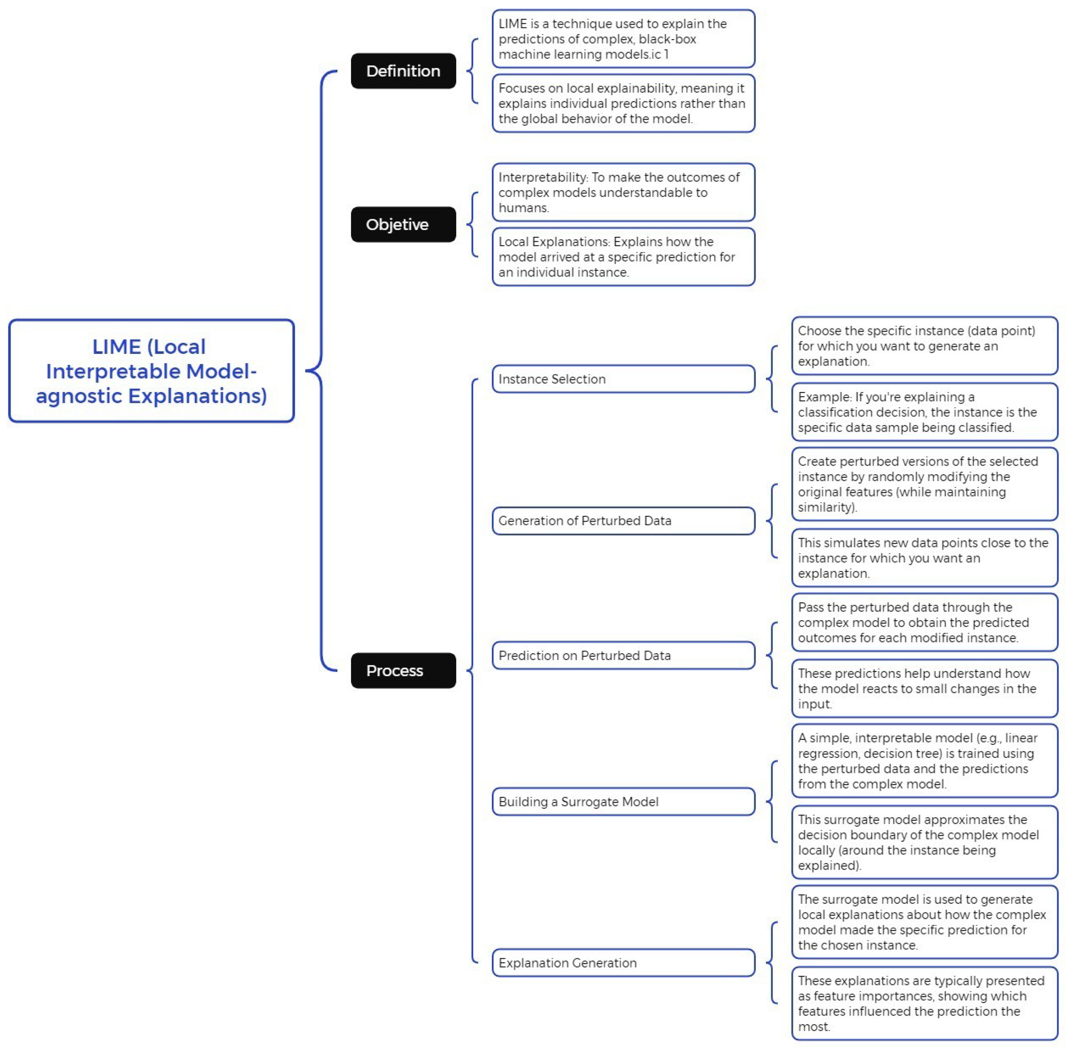
Figure 2.
SHAP: A Model-Agnostic Approach for Machine Learning Explainability
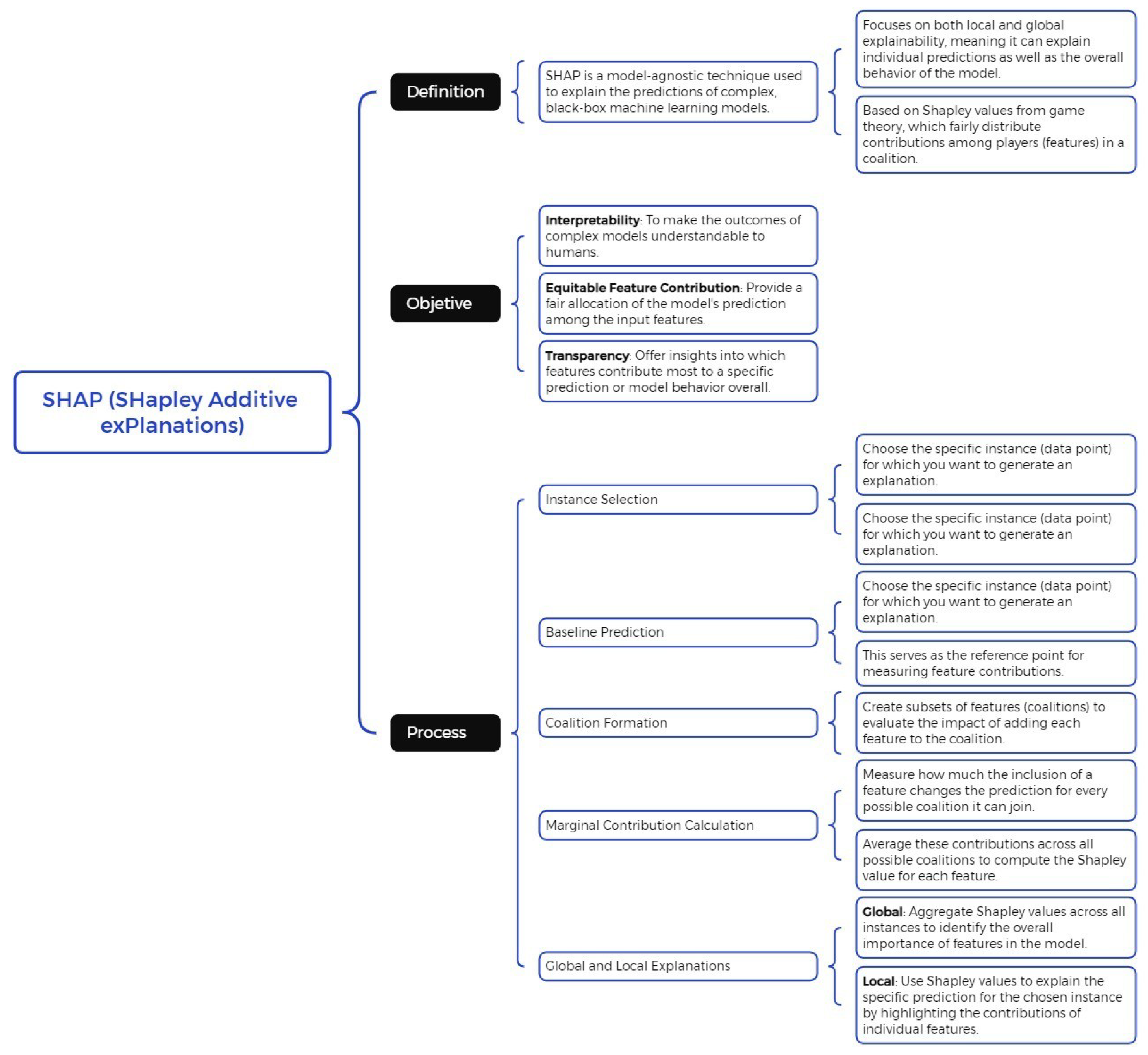
Figure 3.
Comparison of key features between LIME and SHAP.
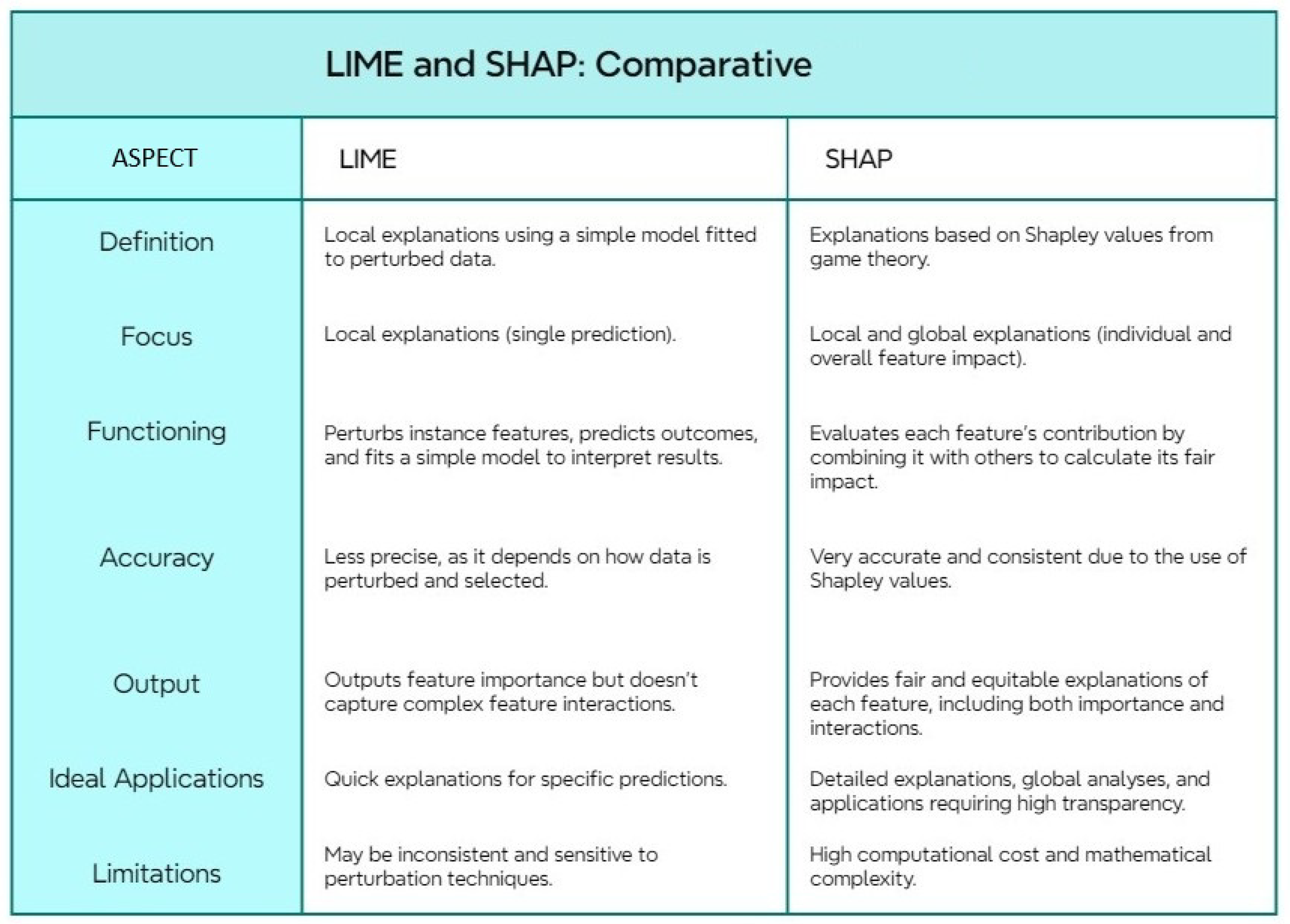
Figure 4.
Diagram of the architecture from UNSW-NB15 dataset.
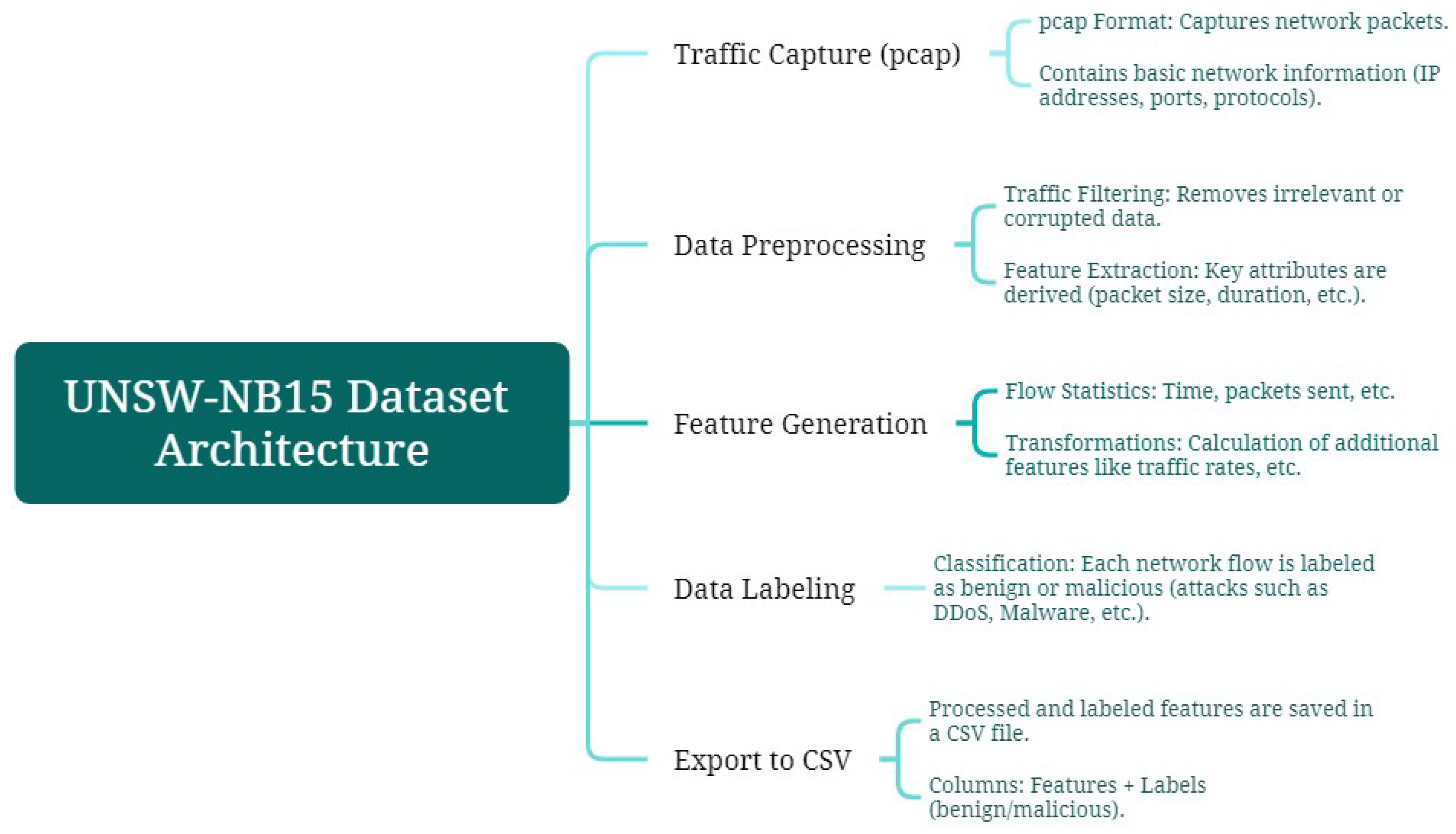
Figure 5.
Diagram of the process order in model training through the UNSW-NB15 dataset and its relation to the SHAP model for explaining decision-making.
Figure 5.
Diagram of the process order in model training through the UNSW-NB15 dataset and its relation to the SHAP model for explaining decision-making.
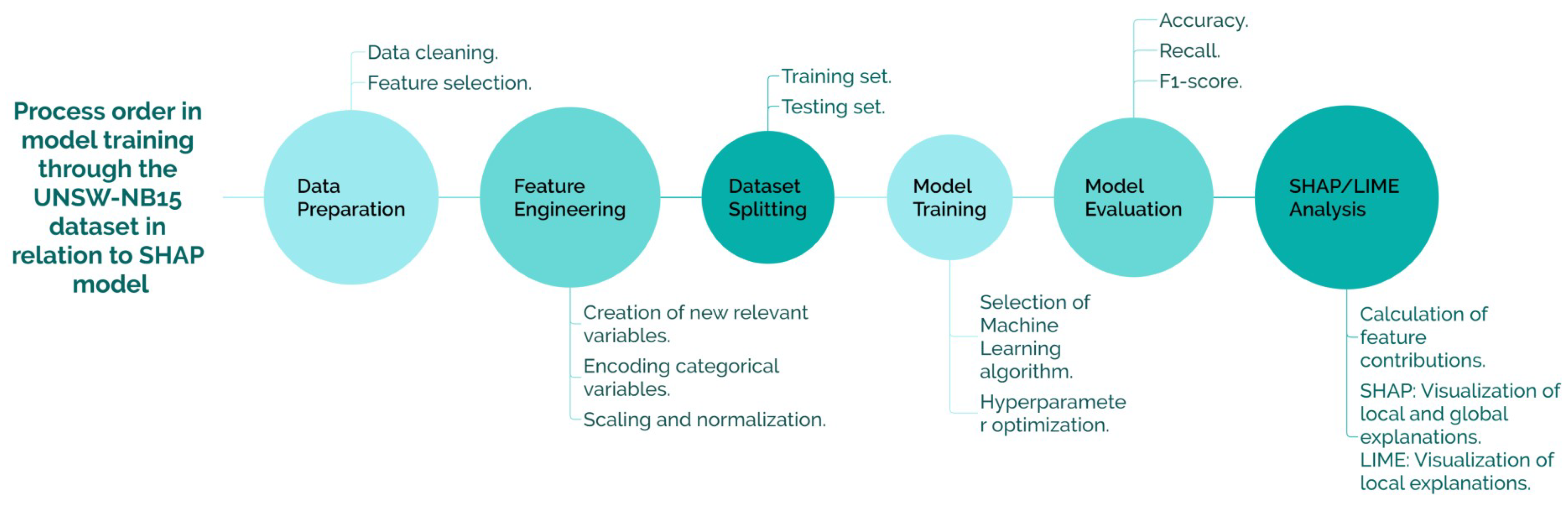
Figure 6.
Confusion matrices for the XGBoost model, presented as percentages.

Figure 7.
SHAP Summary Plot for the XGBoost Model.
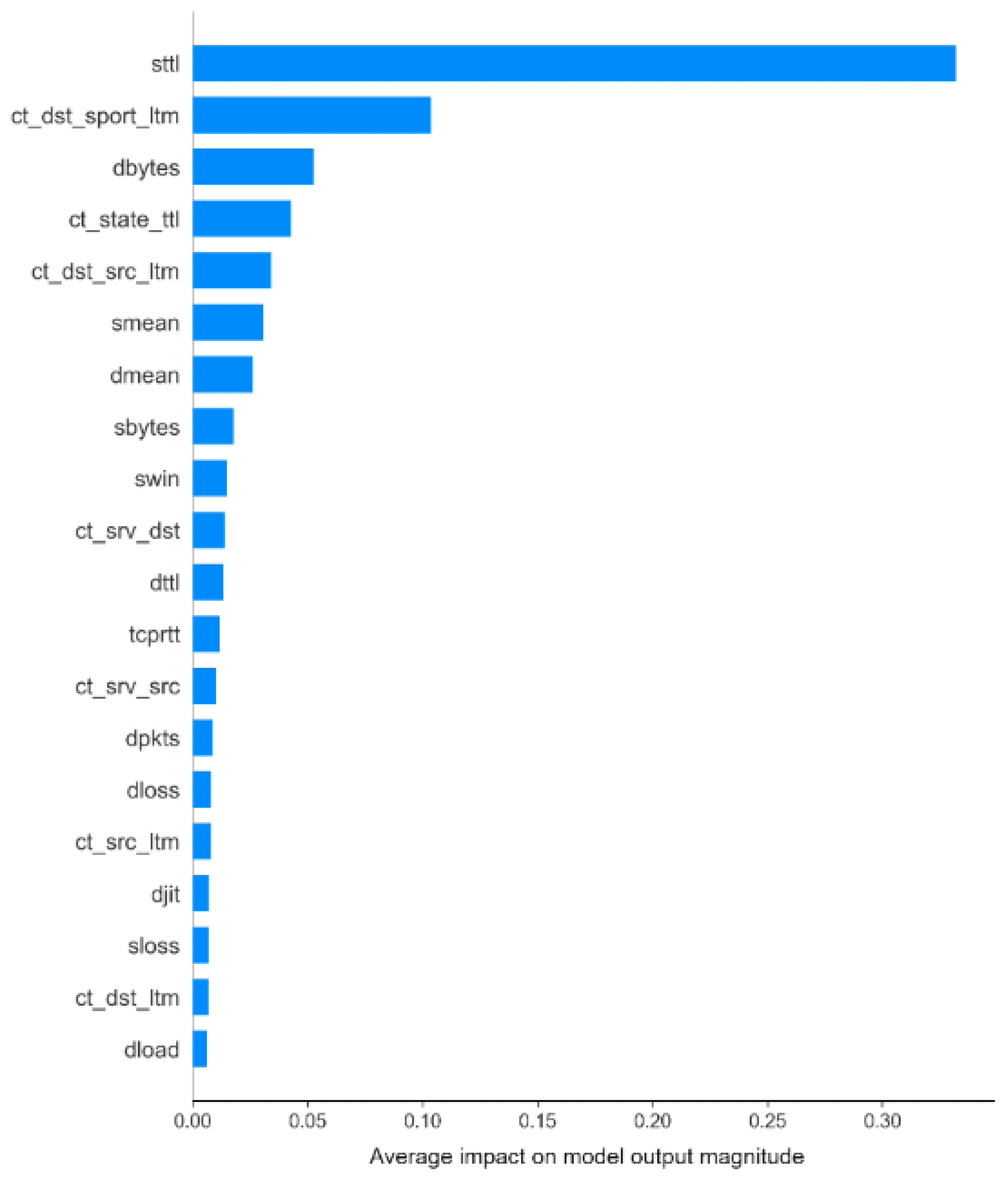
Figure 8.
SHAP Force Plot for instance 15482.
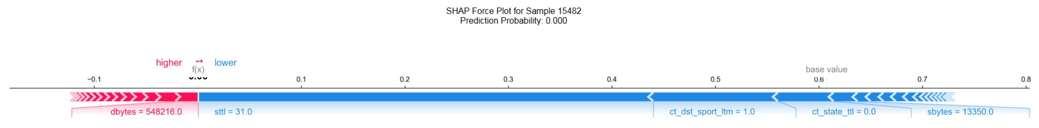
Figure 9.
Explanation of instance 15482 using LIME.
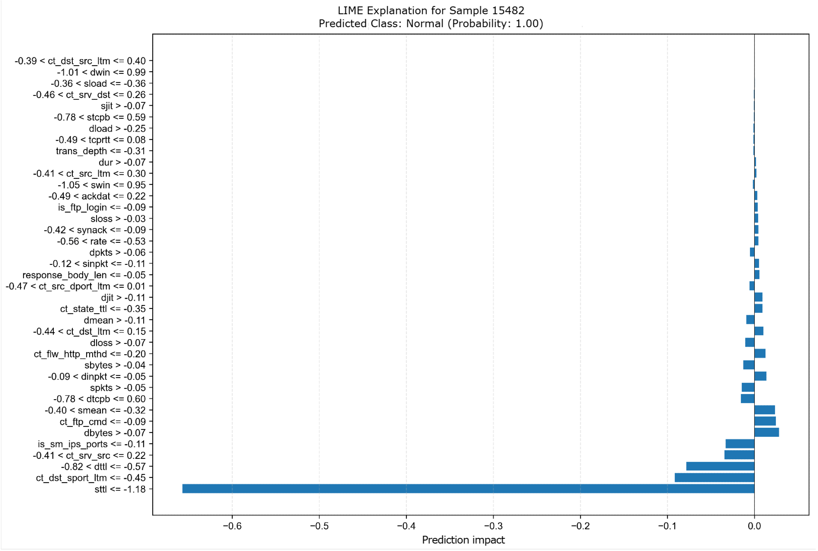
Figure 10.
Confusion matrices for the TabNet model, shown as percentages.
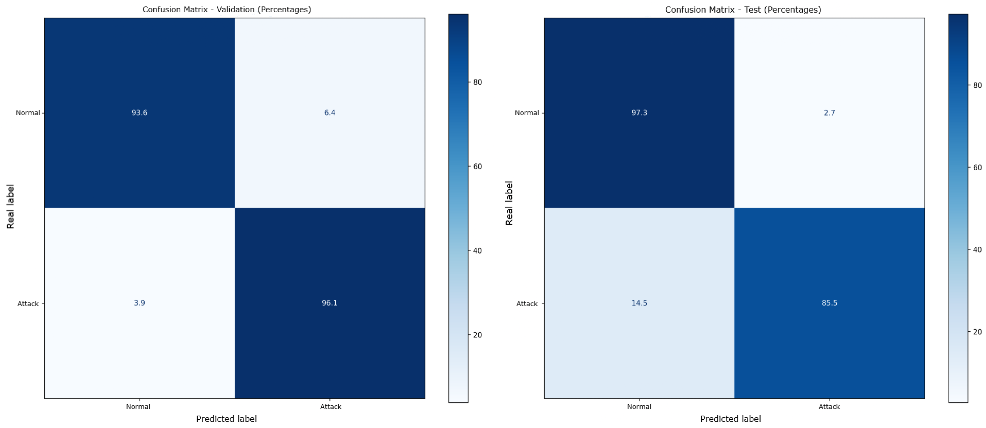
Figure 11.
SHAP Summary Plot for the TabNet model
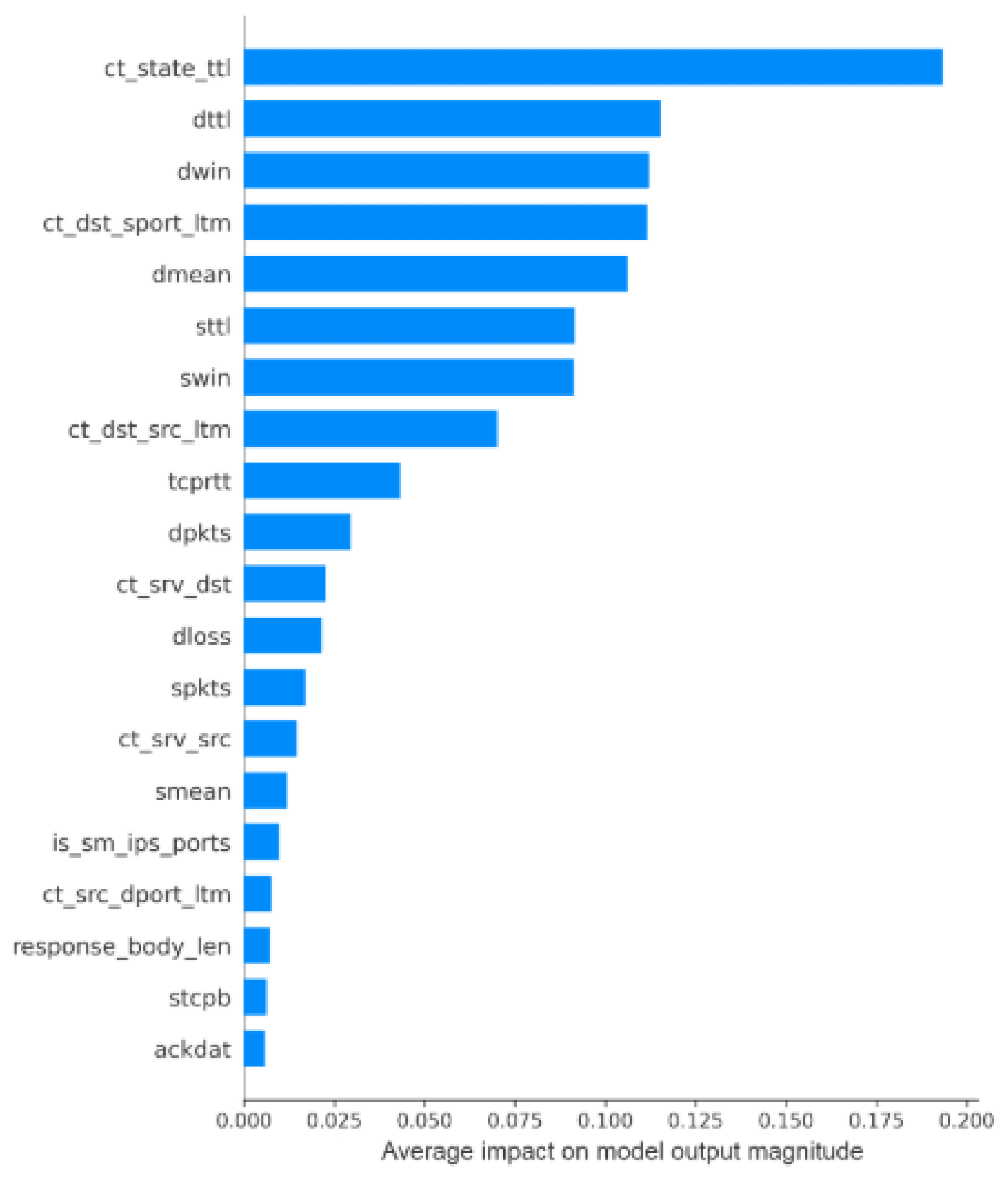
Figure 12.
SHAP Force Plot for instance 29972 using TabNet.
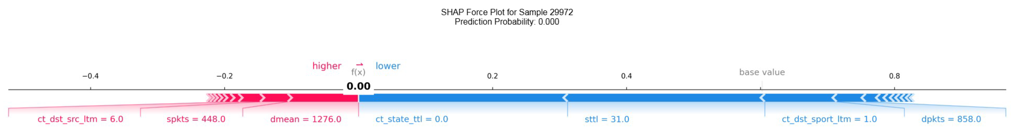
Figure 13.
Explanation of instance 29972 using LIME for TabNet.
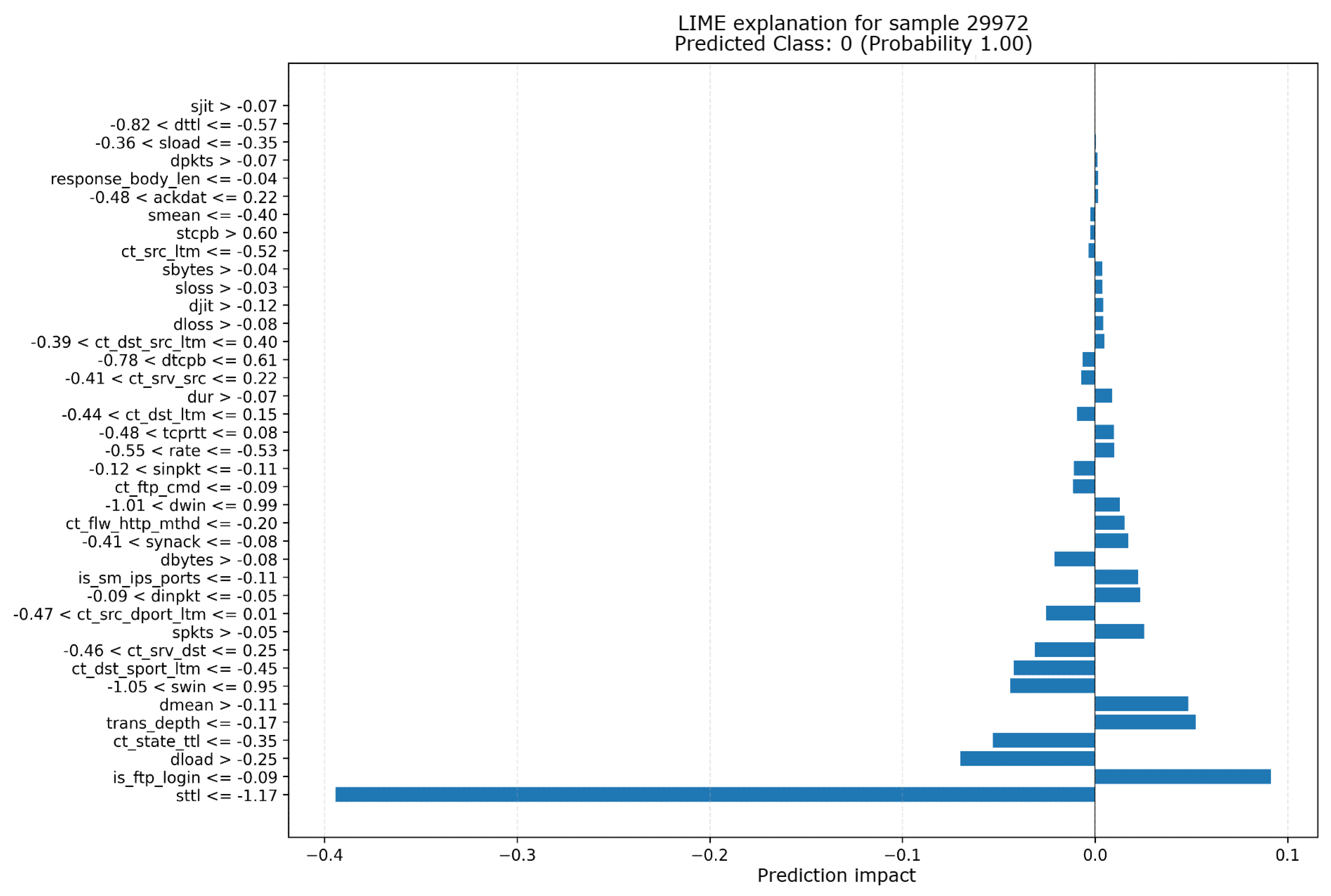

Table 1.
Flow Features
| No. | Name | Description |
|---|---|---|
| 1 | srcip | Source IP address |
| 2 | sport | Source port number |
| 3 | dstip | Destination IP address |
| 4 | dsport | Destination port number |
| 5 | proto | Transaction protocol |
Table 2.
Basic Features
| No. | Name | Description |
|---|---|---|
| 6 | state | Indicates the state and its protocol dependency (e.g., ACC, CLO, and CON) |
| 7 | dur | Total duration of the record |
| 8 | sbytes | Bytes from source to destination |
| 9 | dbytes | Bytes from destination to source |
| 10 | sttl | Source-to-destination time-to-live |
| 11 | dttl | Destination-to-source time-to-live |
| 12 | sloss | Retransmitted or discarded packets from the source |
| 13 | dloss | Retransmitted or discarded packets from the destination |
| 14 | service | Services such as HTTP, FTP, SMTP, SSH, DNS, and FTP-data |
| 15 | sload | Bits per second from the source |
| 16 | dload | Bits per second from the destination |
| 17 | spkts | Number of packets from source to destination |
| 18 | dpkts | Number of packets from destination to source |
Table 3.
Content Features
| No. | Name | Description |
|---|---|---|
| 19 | swin | Source TCP window advertisement |
| 20 | dwin | Destination TCP window advertisement |
| 21 | stcpb | Source TCP sequence number |
| 22 | dtcpb | Destination TCP sequence number |
| 23 | smeansz | Average packet size transmitted by the source |
| 24 | dmeansz | Average packet size transmitted by the destination |
| 25 | trans_depth | Depth in the HTTP request/response transaction connection |
| 26 | red_bdy_len | Size of the content data transferred from the HTTP service server |
Table 4.
Time Features
| No. | Name | Description |
|---|---|---|
| 27 | sjit | Source jitter (ms) |
| 28 | djit | Destination jitter (ms) |
| 29 | stime | Start time record |
| 30 | ltime | End time record |
| 31 | sintpkt | Source inter-packet arrival time (ms) |
| 32 | dintpkt | Destination inter-packet arrival time (ms) |
| 33 | tcprtt | TCP connection setup round-trip time (sum of SYN-ACK and ACK-DAT) |
| 34 | synack | TCP connection setup time between SYN and SYN_ACK packets |
| 35 | ackdat | TCP connection setup time between SYN_ACK and ACK packets |
Table 5.
Additional Generated Features
| No. | Name | Description |
|---|---|---|
| 36 | is_sm_ips_ports | Assigned 1 if srcip equals dstip and sport equals dsport, otherwise 0 |
| 37 | ct_state_ttl | Number of each state based on specific sttl and dttl ranges |
| 38 | ct_flw_http_mthd | Number of flows with methods like GET and POST in HTTP service |
| 39 | is_ftp_login | Assigned 1 if FTP session accessed with user credentials, otherwise 0 |
| 40 | ct_ftp_cmd | Number of flows with an FTP session command |
| 41 | ct_srv_src | Records with the same service and srcip in 100 records based on ltime |
| 42 | ct_srv_dst | Records with the same service and dstip in 100 records based on ltime |
| 43 | ct_dst_ltm | Records with the same dstip in 100 records based on ltime |
| 44 | ct_src_ltm | Records with the same srcip in 100 records based on ltime |
| 45 | ct_src_dport_ltm | Records with the same srcip and dsport in 100 records based on ltime |
| 46 | ct_dst_sport_ltm | Records with the same dstip and sport in 100 records based on ltime |
| 47 | ct_dst_src_ltm | Records with the same srcip and dstip in 100 records based on ltime |
Table 6.
Traffic Type Features
| No. | Name | Description |
|---|---|---|
| 48 | attack_cat | Attack category names (e.g., Fuzzers, Analysis, Backdoors, DoS, Exploits, Generic, Reconnaissance, Shellcode, Worms) |
| 49 | Label | 0 for normal traffic, 1 for attack records |
Disclaimer/Publisher’s Note: The statements, opinions and data contained in all publications are solely those of the individual author(s) and contributor(s) and not of MDPI and/or the editor(s). MDPI and/or the editor(s) disclaim responsibility for any injury to people or property resulting from any ideas, methods, instructions or products referred to in the content. |
© 2025 by the authors. Licensee MDPI, Basel, Switzerland. This article is an open access article distributed under the terms and conditions of the Creative Commons Attribution (CC BY) license (http://creativecommons.org/licenses/by/4.0/).
Copyright: This open access article is published under a Creative Commons CC BY 4.0 license, which permit the free download, distribution, and reuse, provided that the author and preprint are cited in any reuse.


