

Submitted:
06 November 2026
Posted:
09 November 2026
You are already at the latest version
Abstract
Global preservation does not determine what a finite observer can recover. Observer-Dependent En-tropy Retrieval (ODER) makes the passage from preserved encoding to retained possession calculable through causal collection, joint access, and receiving dynamics. For finite Hayden–Preskill sources cou-pled to Schwarzschild propagation and a causal detector, we hold the source, late-radiation apparatus, and collection lifetime fixed. Across all 32 source states, optimal deterministic entanglement-recovery fidelity is at most 0.3308 without early radiation and at least 0.8476 with it. The upper bound applies to every decoder on the available registers, even when decoding computation is unrestricted. A controlled catcher carries this separation into memory; a separate two-site receiver retains a certified separation with finite switching and lossy storage. Independent identical zero-mean Gaussian rail noise admits an exact Pauli–erasure reduction at a specified coherent one-photon interface, yielding deterministic recovery certificates. A separate effective outgoing-field model shows how observer ordering depends on the matched time, incident stream, and receiver controls. Matched spectral trans-mission and mean delay leave finite-window access undetermined. A finite tensor-network (MERA) comparison likewise finds different reference information at identical collection size and individual inclusion probabilities. Removing disentanglers increases mean acquisition under both protocols while reducing their mean difference. Sharp access envelopes and an exact calibration-sufficiency criterion identify the missing information; an additional joint-collection statistic supplies a uniform recovery guarantee. In a five-carrier code, independently erasing collected shares reverses the ranking of two access protocols whose individual efficiencies remain matched. A reference-assisted verification construction shows that preserved encoding and reference erasure induce identical channels below its joint-access threshold and become distinguishable with sufficient access. Once collected, the diary correlations must enter memory and remain there. Uniform capture of an arbitrary collected register gives an exact conditional-mutual-information transfer law in the presence of early side information. Recorded progressive collection extends that channel to randomly admitted registers, with exact infor-mation dynamics and a finite-memory deadline certificate. A centered modular preparation attains the sharp strip-holomorphic activation envelope, and a finite receiver approximates its trajectory with explicit resource requirements. Programmable receiver tests and a staged BEC program connect these constructions to controlled measurements. The resulting standard is physical: the stated data must suffice to establish the claimed recovery or verification performance. The channel constructions determine when that standard is met and which additional measurement can settle an otherwise undetermined claim.
Keywords:
black hole information paradox
; observer-dependent entropy retrieval
; quantum information recovery
; Hayden–Preskill protocol
; operational access
; joint-access calibration
; quantum channels
; quantum memory
; quantum verification
; modular flow
; tensor networks
; analog gravity
1. Principal Findings
Information can survive in black-hole radiation while remaining beyond the reach of an observer who seeks to recover it. Between preservation and possession lies a physical process: correlations must reach the apparatus, arrive in useful combinations, enter memory, and survive until readout. This paper follows that process through explicit quantum channels and determines what the stated physical conditions establish about recovery.
1. Access can limit every decoder, even with unrestricted computation.
Starting from a finite Hayden–Preskill source, the calculation follows the diary through Schwarzschild propagation and an effective causal receiving instrument. The source, late-radiation apparatus, and collection lifetime remain fixed. Changing only possession of early radiation produces nonoverlapping bounds across all 32 source states: optimal deterministic recovery fidelity is at most 0.3308 without early radiation and at least 0.8476 with it. The ceiling applies to every decoder on the available registers. More computation cannot supply the correlations excluded by the observer’s access. (Section 5.2)
2. The retained-information deficit separates exactly into encoding, collection, and transfer terms.
An exact nonnegative decomposition follows the diary through three possible shortfalls: reference information absent from the specified radiation, information excluded by collection, and information available to the receiving system but absent from retained memory. This accounting locates the limitation within the physical chain. Improving a later stage cannot supply correlations excluded earlier. The same ordering separates encoding, supply, and retained-recovery threshold times. (Equation (13); Proposition 19)
3. Familiar apparatus benchmarks can leave recovery undetermined—and additional measurements can repair the guarantee.
Knowing how often each carrier arrives leaves open which carriers arrive together. With individual efficiencies fixed, one admissible collection law caps recovery fidelity at 0.4470 for every frozen source. An additional joint-count constraint instead guarantees at least 0.5190 throughout the resulting law class. The added measurement changes what the calibration can establish. An exact sufficiency criterion identifies when stated statistics determine reference information. The consequences also reach protocol choice: independent share loss reverses which collection protocol performs better at , despite matched terminal carrier efficiencies. (Section 5.9, Section 5.10, Section 5.11 and Section 5.12)
4. Receiving dynamics determine whether collected correlations become durable memory.
The receiving constructions carry imperfect correlations into memory while making acquisition time, routing, switching, and storage part of the recovery guarantee. A controlled catcher preserves the early-access separation after capture. Exact register-transfer identities and recorded progressive collection establish when a scalar transfer law closes and when admission history must remain explicit. The modular construction supplies an exact benchmark attaining the stated activation envelope for a specified preparation; finite receivers approximate that benchmark with controlled error and explicit resources. (Section 4.6Section 4.7, Section 5.5, Section 5.6, Section 5.7 and Section 5.8)
5. Failed recovery cannot distinguish preservation from destruction through an interface that makes them identical.
In the five-carrier construction, preserved encoding and reference erasure induce identical restricted channels below a joint-access threshold. Repetition through that interface cannot distinguish them; sufficient joint access and the declared reference-assisted readout permit discrimination. The retained Hayden–Preskill comparison supplies a quantitative counterpart: equal-prior reference-assisted verification succeeds with probability at least 0.7986 with early radiation, while its optimum is at most 0.559474 without it. The apparatus determines what a recovery failure can establish about the underlying information. (Section 5.13)
Black-hole recovery makes the distinction between preservation and possession unavoidable. The channel, calibration, and verification results apply more generally wherever their assumptions hold. Together, they establish a physical standard: the specified source, apparatus data, and receiving process must establish the performance attributed to the observer.
Readers interested in calibration can begin with joint recovery (Section 5.10); those interested in the evidence for preservation can begin with verification (Section 5.13).
2. Reader’s Guide (How to Read This Paper)
This paper introduces a new way to think about information: not simply as something stored or globally conserved, but as something accessed by an observer in time.
It began with a simple question: What if entropy is not about what exists, but about what becomes accessible to an observer?
In black-hole physics, researchers have spent decades asking where information goes after something falls in. This paper follows the recovery question to the observer: which correlations reach a detector, how they enter memory, and what remains after collection ends. Information can survive in the radiation while a particular observer remains unable to recover it. Following those physical steps makes the distinction between preservation and possession calculable.
The work develops a retrieval account through explicit quantum channels. A finite black-hole diary model shows how propagation and collection determine the information available to an observer. A transfer law describes how admitted information enters retained memory over time. An exact modular construction realizes the law’s extremal activation for a specified preparation, and a finite receiver approximates that dynamics with controlled error and explicit resource requirements.
These calculations lead to measurable questions. How does the same radiation serve observers with different access? What changes when equally efficient detectors collect different combinations of carriers? How much receiving time remains after the information arrives? The experimental program connects these questions to programmable receivers and staged tests in Bose–Einstein condensate analogues.
If you are not a physicist, that is fine. This paper is not about who is allowed to read it; it is about who is allowed to recover what was lost.
The paper is organized as follows:
- Section 4 defines reference-information retrieval and derives the transfer law. Section 4.5, Section 4.6 and Section 4.7 develop the activation bound, exact modular realization, and finite receiver.
- Section 5 follows the black-hole diary through propagation and collection, calculates recovery bounds, and determines what individual collection efficiencies leave unspecified.
- Appendix G provides an interpretive aid. Appendices Appendix H, Appendix I, and Appendix J give the access, modular, and receiver proofs. The computational companion reproduces the numerical calculations.
3. Introduction
A quantum diary falls into a black hole. If its information survives in the outgoing radiation, what has been established for an observer who seeks to recover it? Preservation concerns the global evolution. Recovery requires access to the correlations carrying the diary, and retained possession requires those correlations to enter a physical memory. The distinction matters whenever failure to recover information is taken as evidence that the information has been destroyed.
Hawking’s derivation of particle creation and his subsequent argument for a breakdown of predictability concern the global evolution of a black hole and its radiation [1,2]. Observer-Dependent Entropy Retrieval (ODER) follows the recovery claim through the physical observer. A finite unitary encoding supplies a controlled starting point: a guarantee for a radiation subsystem must be evaluated after collection has restricted that subsystem to the available registers and receiving dynamics have transferred it into memory. We call the apparent contradiction produced by identifying global preservation with observer possession the operational-access form of the information paradox. ODER dissolves that contradiction by calculating how the same preserved encoding supports different recovery outcomes. Access and acquisition determine those outcomes, so they belong within the physical statement of recovery.
The physical comparison holds the source state, late-radiation detector, and collection lifetime fixed. Only the observer’s possession of existing early radiation changes. Across the 32 tested source states, branch-resolved bounds place optimal deterministic entanglement-recovery fidelity at most without that early radiation, while access to it permits fidelity of at least . The restricted observer’s ceiling applies to every deterministic decoder acting on the available registers, with unrestricted decoding computation. The earlier radiation provides the correlations that make the arriving radiation useful for diary recovery. Fixed-preparation transmission controls further isolate the Schwarzschild channel: attenuation and scattering phase change the finite-window recovery bounds, while the early-radiation separation persists in each tested condition.
Even after the Schwarzschild propagation is fixed, the path to the detector can change what the observer receives. We follow that propagation with either a lossless dispersive element or a matched pure delay. The resulting causal channels have identical spectral transmission and the same spectrum-weighted mean group delay. They nevertheless deliver different reference information to the fixed observer before the deadline. In the dispersive arm, mean full-early reference information is lower by than in the matched-delay arm. Frequency-dependent phase reshapes the arriving packets, changing which existing diary correlations reach the receiving apparatus in time. Spectral attenuation and one delay number therefore leave this recovery task undetermined, even after the Schwarzschild propagation has been fixed. Section 5.4 constructs the causal comparison and retains the magnitude-only phase diagnostic as a separate control.
Knowing how often each carrier arrives still leaves a question: which carriers arrive together? Two collection protocols can match every individual efficiency while making different diary correlations available. Proposition 15 gives an exact row-space criterion for when the calibration statistics suffice to determine reference information. The recovery certificates show what this omission can cost. Fix all ten early and late collection probabilities, with early marginals . One common source-independent collection law then caps optimal fidelity at for every tested source. Adding the measured condition that at least two late and four early carriers are jointly collected with probability at least instead guarantees fidelity at least throughout the resulting law class (Section 5.10). The added statistic repairs a guarantee that individual efficiencies cannot supply. The five-carrier code makes the role of storage especially direct: independent share loss reverses which of two collection protocols performs better, although every carrier has the same terminal inclusion probability under both protocols. Joint access therefore determines which collection strategy survives a specified storage process.
A finite-MERA comparison fixes collection size as well: both protocols acquire exactly three sites and include every site equally often, yet contiguous access yields more reference information in all 64 sampled encodings. In the ensemble comparison, paired removal of the disentanglers reduces the contiguous-access advantage while raising acquisition under both protocols. The access pattern therefore probes the encoding’s correlation structure. Reference-assisted verification gives the distinction a further operational consequence: in the five-carrier construction, preserved encoding and reference erasure induce identical channels for unauthorized access, while sufficient joint access permits their discrimination (Section 5.13). A failed recovery attempt alone cannot decide between these physically different global processes.
The next physical requirement is acquisition before the receiving interaction ends. A controlled catcher converts the detector output into retained memory and preserves the fixed-source separation, with bounds and (Section 5.5). Uniform transfer of an arbitrary collected register then gives an exact law for the additional reference information acquired alongside an already held early register (Section 5.6). A recorded progressive receiver further freezes a selected arriving subset, transports it without first decoding the diary, and gives an exact cohort formula and a five-level-per-site receiving example (Section 5.7). The diary correlations now have a physical route from the source into retained memory. How quickly can that acquisition occur? Within the strip-holomorphic activation class, Proposition 10 gives a sharp earliest acquisition time at fixed supply and kinetic rate, and Proposition 20 determines whether the remaining interaction can reach a chosen target. A vacuum modular boost realizes the extremal tanh activation for a centered wavepacket and a fixed source–memory partition. Its hyperbolic disk coordinate connects the modular orbit to the exact transfer channel; preparation and receiver changes provide explicit tests of class membership.
The modular construction also admits a finite receiving model. Constant nearest-neighbor couplings transfer a coherent diary into a finite memory, with uniform bounds on the departure from the exact modular trajectory and its activation. Disconnecting the source at the acquisition deadline preserves the captured information in the lossless model. At fixed generator variance, the centered member of the translated preparation family acquires at least as much reference information at every time (Appendix I.6). This comparison identifies the resource dependence of the preparation advantage.
A separate two-site receiver makes finite switching and storage loss explicit (Section 5.8). Applied to the 32 Hayden–Preskill sources, it permits retained recovery fidelity at least with early radiation, while every decoder without it remains bounded above by . The corresponding reference-assisted verification scores are at least and at most . With the encoding and collection channel fixed, changing storage loss can also determine whether a chosen retained-fidelity target can be reached. These are physical differences in the state available at readout. Section 8.5 further examines how a serial receiver divides its available duration between collection and capture. Together, the constructions put the challenge directly: the physical data offered for a recovery claim must establish the performance attributed to the observer.
From Radiation Entropy to Observer Recovery
Island and replica-wormhole calculations have been presented as resolutions of the information paradox within specified gravitational models [5,66]. Their results determine radiation entropy and support reconstruction statements for selected radiation regions [3,4]. The region and operations in each result determine the information available for reconstruction. Physical recovery then requires a collection channel and a receiving system. Section 5 evaluates the collection step for a controlled unitary source, with recovery bounds optimized over every deterministic decoder on the collected registers.
The channel theory in Section 4 makes acquisition a dynamical question. A recorded instrument with specified branch fidelity and decoupling gives the remaining-gap law. Its solution weights incoming supply by the acquisition opportunity available after arrival. The resulting deadline criterion connects a recovery target to the duration and strength of the receiving interaction. Section 7 develops direct receiver tests and BEC measurements of the associated access relations.
The operational chain is
The first relation records global encoding in the radiation algebra. The first arrow restricts that encoding to what can causally reach observer i. The second requires a receiving interaction that transfers reference information into retained memory.
The reference Q identifies the diary information throughout the comparison. We write for its encoding in the specified radiation, for the supply available to observer i, and for the fraction retained in memory. A late increase in supply cannot replace acquisition time that has already elapsed. This timing constraint becomes quantitative through the remaining transfer dose in Section 8.4.
For the recorded transfer family, describes activation at detector setting b, and is the resulting transfer rate. The activation bound determines the earliest crossing of the positive-coherent-information boundary within this family.
Local quantum-field algebras remain Type III in the continuum [20,30]. A split inclusion provides a regulated Type-I factor on which density-operator expressions may be used, while Araki relative entropy remains the primary definition. The split distance regulates the algebraic representation. Finite switching, spectral response, and detector resolution define the observer protocol.
Physical setting. The black-hole calculation combines a unitary finite Hayden–Preskill source with asymptotic Schwarzschild scalar transmission and a causal passive detector. The transfer theorem applies to the stated recorded instrument. The modular benchmark specifies a vacuum wedge group, finite-energy packet and fixed modal memory; its finite-chain realization uses a laboratory clock calibrated by the couplings. The controlled catcher composes the source and collection channel with retained storage; the uniform-register receiver supplies a further acquisition channel for imperfect collected input and early side information. Each construction states its apparatus and time budget. Split regularization supplies Type-I representatives for restricted field algebras. Detector bandwidth and acquisition duration remain physical protocol inputs.
The table below maps the paper’s results to their mathematical basis and operational measurement or test. It distinguishes derived conclusions from the assumptions, calibrations, and observation models used to obtain or test them. The Ground column links directly to the relevant definitions and derivations; the final column identifies measurement routes and proposed tests. Appendix G provides the accompanying physical interpretations.

Table 1.
Results, derivations, and measurement routes.
| Object | Status | Ground | Operational measurement or test |
| Table 1: Results, derivations, and measurement routes (continued) | |||
| Object | Status | Ground | Operational measurement or test |
| Continued on the next page | |||
| Observer access and recovery | |||
| Defined | Reference mutual information, Eq. (6) | Reference-tagged memory | |
| Derived | Data processing, Eqs. (11) and (15) | Cross-protocol ceiling | |
| Calculated for finite sources; supplied in general theorems | Causal observer construction, Section 5 | Reference-tagged source and accessible-state estimate | |
| Deterministic recovery fidelity | Branchwise bounds for every frozen HP source | Corollary 9, Section 5.2 | Available mask flags and deterministic Bell overlap |
| Gaussian noise and logical recovery | Exact reduction for the specified rail class and readout; propagated recovery bounds | Section 5.3 | Identical independent zero-mean rail channels, coherent total-one-photon readout, and all-trial Bell overlap |
| Recovery under uncertain joint collection | Computed certificate bounds and a joint-count repair | Section 5.10; Appendix H.6 | Component marginals, simultaneous collection records and calibrated flag readout |
| Calibration sufficiency | Derived exact row-space criterion | Proposition 15 | Declared calibration statistics and additional joint measurements |
| Reference-assisted verification | Exact restricted-channel equality and access-dependent discrimination | Proposition 17; Section 5.13 | Retained reference, joint carrier access, and deterministic verification score |
| Causal propagation at matched transmission and mean delay | Analytically specified causal channels; numerical information separation at one resonator setting | Eqs. (117)–(118); Table 5. Independent causal integration agrees within in waveform amplitude | Collected probability and reference information for dispersive and matched-delay arms; fixed preparation, detector, and deadline; 32 source states |
| Finite-MERA fixed-cardinality access comparison | Constructed encodings; numerically resolved ensemble and paired ablation | Section 5.11; 64 MERA/tree pairs and 64 independent Haar encodings; architecture and exact-null checks in Appendix C.1 | Reference-tagged three-site collection with equal inclusion probabilities and a recorded subset flag; eight sites, bond dimension two, random unoptimized tensors |
| HP access-correlation envelope | Numerically sharp in declared family | Fixed-marginal optimization, Section 5.9 | Component marginals and joint access records |
| Exact QEC access and recovery envelope | Derived; sharp endpoints attained at fixed carrier efficiencies | Five-carrier erasure code, Section 5.12; Eq. (150) | Joint collection records and deterministic entanglement-recovery fidelity |
| Encoding-dependent access ordering | Exact QEC comparison; reversal calculated for all 32 HP sources | Same mask laws and common marginal , Section 5.12; fixed late detector for HP | Compare exactly-three and all-or-none access while matching each carrier’s efficiency |
| Noise-dependent access ordering | Exact crossover at active-share survival | Proposition 16; Appendix H.9 | Fixed encoding and installed receivers; matched terminal marginals; vary independent share loss |
| Static and infalling observer comparison | Conditional recovery separation and channel ordering in a specified effective model | Section 5.15 | Compare equal proper duration, equal incident stream, and additional resonance and coupling controls |
| Transfer dynamics and analytic limits | |||
| Controlled catcher | Explicit retained channel and certified HP recovery separation | Section 5.5; Eqs. (120) and (123) | Controlled coupling, retained reference information, and deterministic recovery fidelity |
| Imperfect-register transfer | Exact conditional-information law | Section 5.6; Eqs. (126) and (127) | Uniform capture of the collected register with early side information |
| Progressive register capture | Exact recorded-cohort channel; common-clock scalar law; finite-chain deadline certificates | Proposition 14; Table 6 | Accepted-time records, fixed-size routing, early side information, and designated receiving memory |
| Finite switching and noisy storage | Exact receiving channel and propagated HP recovery and verification bounds | Section 5.8; Appendix J.4 | Smooth source isolation, calibrated loss, holding duration, and all-trial reference readout |
| Operational output sectors / flagged approximation | Orthogonality derived; branch conditions supplied or verified | Proposition 4 | Readout-outcome fidelity and decoupling audit |
| Finite/Lindblad gap law; unitary balance | Exact | Flagged CPTP/GKSL laws and Proposition 6 | Retrieval trajectory and R–M– reference audit |
| Coherent-information boundary | Exact for flagged family | Corollary 2 | Reference-tagged threshold at |
| , real monotone trace | Supplied or verified in general | Analytic hypothesis, Section 4.5; realization in Section 4.6 | Independent activation construction or protocol-level verification |
| bound and tanh | Derived; exact extremizer | Strip Schwarz–Pick result, Eqs. (57) and (59) | Independent activation trace |
| Proper-time tanh | Derived with affine clock | Clock calibration, Eq. (62) | Onset timing |
| Clock-dose invariance | Derived; exact | Proposition 8 | Cross-clock dose consistency |
| Checkpoint envelope, contact rigidity, activation delay | Derived; sharp | Proposition 9 | Pairwise activation trace |
| Cosh-power trajectory / sharp envelope | Exact equality branch / derived sharp envelope | Eqs. (67) and (69) | Threshold timing and onset/tail tests |
| Clock ordering, supply overlap, terminal dose | Derived corollaries | Eqs. (179), (52), and (185) | Schedule swap and finite-lifetime test |
| Exact modular realization and finite receivers | |||
| Specified modular transfer channel | Derived; exact | Fixed modal partition and erasure channel, Eqs. (A146)–(A152) | Coherent diary preparation and access to the stated memory modes |
| Modular activation and disk extremality | Derived for centered preparation | , ; Eqs. (A158)–(A160) | Normalized transfer hazard with specified modular clock |
| Preparation-dependent departures | Derived; exact within translated family | Monotonicity, overshoot, and strip-class violation, Appendix I.5 | Controlled source displacement and activation trace |
| Modular rate and proper-time scale | Derived with specified clock | , , Eq. (A161) | Packet shape and physical clock or coupling scale |
| Finite-receiver accuracy | Derived; uniform on | Proposition A9; resource bound (A187) | Finite-chain transfer and activation traces over the certified interval |
| Deadline retention | Exact under disconnected, lossless dynamics | Source-link disconnection, Appendix J.3; error budget (A188) | Retained reference information and storage-loss characterization |
| Geometric response, calibration, and observation | |||
| Retrieval–curvature response | Derived conditional on supplied source | Appendix D.1 and Eqs. (275)–(A85) | Focusing and threshold-shift response after coupling calibration |
| Calibrated or inverse-inferred | Transfer protocol and Eq. (56) | Retrieval trace plus | |
| Specified or calibrated in general | Eq. (53); modular value in Eq. (A161) | Independent kinetic or activation benchmark | |
| External calibration or nuisance | Tagged sensitivity in Eq. (170) | Observation model | |
| map | Projected | Observation hypothesis, Eq. (170) | Density correlations |
| Tier 0 archive and processing operators | Supplied and registered | Data provenance and paired analysis paths, Section 7 | Minimally aggregated and conventional correlation surfaces |
The exact modal realization and the finite-chain certificates have distinct domains. The latter control real-time trajectories on the stated interval; they do not establish global strip-to-disk membership for finite activation.
3.1. Relation to Algebraic Entropy and Crossed-Product Constructions
Recent work in algebraic quantum field theory has clarified a foundational issue underlying gravitational entropy: how entropy may be meaningfully defined for systems whose local algebras are Type III and therefore admit no trace. In particular, crossed-product constructions developed by Chandrasekaran, Penington, and Witten, building on earlier modular and algebraic work by Longo and Takesaki, give rigorous constructions in which entropy is finite and well posed for quantum field theories with gravitational relevance [21,30,32,33].
These results resolve definability: what it means for entropy to exist as a mathematical quantity in relativistic quantum systems where density-matrix notions fail.
Crossed-product and related algebraic constructions establish the algebraic status of entropy and modular structure. This paper asks how diary-reference correlations enter a finite observer’s retained memory through a specified physical channel. Relative-entropy mutual information follows those correlations across collection and acquisition. The transfer dynamics supply rate and proper-time conditions for that task.
3.2. Operational–Access Criterion and Relation to Recovery Literature
The operational-access criterion asks whether the stated physical data establish the asserted recovery conclusion. An exact score must be fixed by those data; a guaranteed bound must hold across the realizations they permit. An existence claim instead requires an admissible construction. This criterion locates the substantive step in moving from information encoded in radiation to recovery by an observer: the accessible state and receiving process must support the conclusion being drawn. A change in joint access can reverse that conclusion with the source, late-radiation apparatus, and collection lifetime held fixed.
The required specification follows the task. Deterministic decoding concerns the state delivered to the decoder. Retained retrieval also concerns transfer, storage, and the available proper-time interval. Verification concerns the distinguishability of specified hypotheses through the permitted measurements. The exact calibration-sufficiency criterion and sharp access envelopes below determine when partial observer data already establish a result and when an omitted correlation changes the answer. They turn the distinction between global preservation and physical possession into a test of the recovery claim itself.
Black-hole information recovery is the forcing case for this question: preservation, causal collection, retained memory, and verification must be specified separately. The access and receiving-channel results apply wherever their stated assumptions hold, including outside a gravitational setting. The black-hole calculation gives those general relations a physical instantiation with specified propagation, apparatus, and deadlines.
Hayden and Preskill formulate diary recovery using early and late radiation, with extensive control of the emitted radiation as an explicit assumption [7]. Bao and Kikuchi directly study how erasure and decoherence of stored early radiation affect decoding [38]. These results make side information and its degradation part of the operational problem. The present calculation connects a finite source from this lineage to complex Schwarzschild propagation and a passive, causal observer instrument. It evaluates the resulting diary-reference information, certifies a separation in optimal deterministic recovery quality, and determines which conclusions survive incomplete knowledge of access correlations.
Operational questions also arise explicitly within island research. Modular-flow extraction provides a procedure for accessing island information under specified control of the radiation modular Hamiltonian [67]. Observer-defined entropy calculations model absorption into a fiducial detector and relate the entropy prescription to the observer’s worldline [68]. Geometric analyses of decoding complexity examine the computational cost of extracting encoded information [69]. These results distinguish several operations that the word “recovery” can denote.
The recent exchange between An apologia for islands and Seeing Page Curves and Islands with Blinders On places the choice of accessible observables at the center of this issue [8,9]. Antonini et al. propose coherent collection into waveguides, fault-tolerant storage, and repeated tomography or permutation measurements. Their robustness argument specifies a noisy collection channel, approximate factorization over temporal bins, and a small environment-entropy condition. Geng et al. argue that omitting the Hamiltonian from the exterior algebra changes the information question and challenge the physical realization of that restriction at finite radius.
ODER applies the operational-access criterion to the asserted measurement: which output channel realizes the chosen observables, which correlations survive collection and storage, and which hypotheses can its measurements distinguish? Copy number, cross-copy control, and storage duration belong to that specification. Collection and subsequent measurement have separate deadlines; retained radiation can be measured after evaporation. For the exact restricted-channel equality in Proposition 17, repeated uses of the same interface preserve equality, including joint measurements across copies. Repetition cannot distinguish identical channels. This is a precise access obstruction to verification, while nonzero distinguishability can accumulate across copies. An entropy curve, a recovery certificate, and a test of reference preservation therefore require their respective operational conclusions to be established on the channel actually available to the observer.
Harlow and Hayden connect the feasibility of an AMPS thought experiment to the computation needed to decode early radiation, arguing that this computation can exceed the black hole’s lifetime [10]. The shared operational question is whether an observer can complete the required task in time. Here the access bounds allow unrestricted decoding computation and constrain the state delivered to every decoder. Collection, joint access, and retained acquisition therefore supply distinct restrictions, while the finite receiving construction makes their time and coupling costs explicit.
The present access bounds concern the input to every decoder. They quantify the correlations delivered by the collection channel, including the dependence on which carriers arrive together. Complementary receiving constructions follow reference information into finite memory, with quantitative acquisition bounds and a disconnection operation that retains the captured information under lossless storage.
Recent experiments and local-recovery benchmarks make the comparison more specific. Bang et al. implement finite-temperature Hayden–Preskill recovery on an IBM processor and measure both postselection probability and conditional fidelity [43]. Our deterministic Bell-overlap score includes every outcome. For a common output task, a probabilistic protocol contributes
so conditional fidelity alone does not determine the corresponding deterministic performance. Their implemented decoder and our bounds on all decoders supply complementary information about recovery.
An, Cao, and Cui distinguish target-only recovery, bounded-depth recovery on a finite window, and optimal recovery from that same window [44]. Their comparison separates access to a larger subsystem from the control needed to use it. In the present HP calculation, the collection deadline fixes the accessible registers, while the recovery bounds allow unrestricted computation on them. The lower bound certifies the existence of a decoder on those registers. Its implementation has an additional control and execution-time budget, while Section 4.3 specifies the receiving instrument.
Can and Wilde give one-shot entanglement-generation and distillation bounds using Petz recovery and binary hypothesis testing [49]. Their state-dependent decoding channel also acts on an arbitrary received joint state, providing an explicit candidate for the fixed-state task considered here. The present comparison holds the diary encoding fixed and changes its physical collection: the resulting state sets both the ceiling on every decoder and the achievable lower certificate. The branch-resolved bounds below retain the collection record when forming that certificate. Coding achievability and physical collection thus meet at the received state; the transfer construction follows its reference information into memory over a specified receiving interval.
Zhang and Chen characterize a different operational requirement [50]. A channel preserves every finite incompatible measurement family under its adjoint exactly when an isometry W satisfies for every d-dimensional state. The channel itself then outputs the encoded state without a further recovery map. Our observer comparison fixes the source and evaluates a particular diary reference after collection, including cases with partial recovery. This distinguishes universal preservation of measurement incompatibility from the reference-specific access and finite-time acquisition calculated here. The finite-MERA comparison tests the latter at fixed collection size and component inclusion probabilities.
The mathematical ingredients also have established operational meanings. Conditional min-entropy characterizes optimal entanglement recovery by local decoding [40]; we apply that identity and relative- entropy data processing to the calculated observer states. Quantum secret sharing and erasure correction identify authorized collections of carriers [11,41]. The five-carrier construction uses that structure to derive exact bounds at fixed component reliability. The physical composition exposes freedoms that global encoding and component efficiencies leave unresolved. The resulting bounds identify when those freedoms alter recovery, which additional measurements determine it, and how the accessible correlations enter retained memory.
Table 2.
Applying the operational-access criterion to selected results. The final column identifies the physical specification needed to carry each result into an observer recovery or verification claim.
Table 2.
Applying the operational-access criterion to selected results. The final column identifies the physical specification needed to carry each result into an observer recovery or verification claim.
| Result or construction | Established conclusion | Access dependence of the physical claim |
|---|---|---|
| Page, island, and replica calculations [3,4,6] | Entropy and, where established, reconstruction for specified subsystems | The available channel must connect those subsystems to the observer’s recovery task |
| Hayden–Preskill [7] | Diary recovery with joint control of early and late radiation | Physical collection determines whether the required joint state reaches the decoder |
| Noisy early radiation [38] | Decoding with degraded early side information | The joint early–late access law determines the received correlations |
| Harlow–Hayden [10] | A computational obstruction to the decoding step in the AMPS protocol | The state offered to that computation already depends on collection and retention |
| Page-curve observation [8,9] | Proposed collection and entropy measurements; competing accounts of the accessible algebra | The realized restriction, storage errors, copy resources, and measurement specify the observable evidence |
| Conditional min-entropy and Petz recovery [40,49] | Optimal recovery characterization and explicit state-dependent decoding bounds | Applying either result requires the joint state produced by the collection channel |
| Quantum secret sharing [41] | Exact recovery from authorized subsets | Individual efficiencies leave the probability of joint authorization undetermined |
| Incompatibility preservation [50] | A universal channel criterion equivalent to a noiseless encoding | Reference-specific partial recovery requires the chosen source and actual access channel |
The access envelope decides when the observer description is sufficient for the claimed conclusion. An interval entirely on one side of the coherent-information boundary certifies that regime even when the exact score remains undetermined. An interval that straddles the boundary leaves the regime unresolved by the stated measurements. The missing joint-access information then changes the physical answer. The criterion thus tests the inference from a supplied description to a recovery claim, rather than requiring a complete reconstruction of every receiver detail.
The retained-transfer theorem addresses the passage from accessible correlation to possession. The modular construction makes that passage explicit in a coherent erasure channel, using a known modular return amplitude and its Krylov representation [63]. The finite receiver converts the representation into constant nearest-neighbor acquisition dynamics. Its certificate quantifies how finite hardware approaches the exact trajectory. These constructions connect the access problem to a specified memory process.
3.3. Retrieval, Reconstruction, and Comprehension
[nobreak=true] Throughout this work we distinguish five questions about information:
- Preservation: persistence of the diary information under the global evolution.
- Encoding: correlation of that information with radiation or another exterior carrier.
- Retrieval: transfer of causally available reference information into retained observer memory.
- Reconstruction: the existence of a formal decoding map or entanglement-based reconstruction channel.
- Comprehension: the observer’s ability to interpret or act on retrieved information.
Each question has its own criterion. ODER derives the retained-retrieval dynamics: the transfer of causally available reference information into observer memory. The physical chronology of encoding, causal admission, and retained acquisition is established in Proposition 19.
The corresponding distinctions are
The constructions meet at a common physical question: what happens to the diary’s correlation with its reference as radiation is collected, transferred, and retained? Following that same correlation across the interfaces makes it possible to locate a recovery obstruction and ask what change would remove it. A failed recovery can then be traced to the encoding, the available carriers, or the receiving process, while a verification experiment asks whether the observer has enough evidence to distinguish preservation from erasure. This is the passage from preservation to possession that ODER makes calculable.
4. Observer-Dependent Entropy Retrieval
To follow the diary from radiation into memory, we need a measure that keeps track of the same information throughout. Correlation with an untouched reference provides that continuity. We first measure how much reference information the observer can collect, then follow its transfer into retained memory.
4.1. Reference-Defined Retrieved Entropy
Throughout, logarithms are natural and we use units unless stated otherwise.
The reference fixes the information being followed. It remains outside the transfer process and records whether the diary correlation has reached the observer’s memory.
Let be a diary initially purified by a reference . For the exact channel construction below the initial state is maximally entangled,
For any identified d-dimensional data register X, write . The linear formulas in Section 4.3 use this maximally entangled input and the orthogonally flagged channel defined there.
In algebraic quantum field theory, a local observable algebra need not admit a density matrix. For normal states and on the relevant von Neumann algebra, define
where is Araki relative entropy [31]. This is the primary modular-algebraic information quantity.
For split-regularized localization we assume a split inclusion
where is a Type-I factor and is a spatial split distance [29]. On that regulated factor, Eq. (3) has the density-operator representation
When the individual von Neumann entropies are finite, this reduces to . The relative-entropy definition remains primary when those separate entropies are infinite. The split property provides the regulated factorization. The observer protocol fixes the detector cutoff. These are independent controls: regulates localization, while the detector passband fixes the operational spectral window.
Definition 1
(Reference-retrieved entropy). For observer protocol i, let be the retained quantum memory through proper time τ. Define
For a perfect purification transferred to memory, and . Equation (6) measures diary correlation, with the controlled diary entropy as its ceiling. Memory entropy and black-hole entropy measure different objects.
Reference information tells us how strongly the memory remains correlated with the diary’s reference. Recovery fidelity asks how well a decoder can reconstruct the diary from that memory. Verification asks a further question: can the available measurements distinguish preserved reference correlations from erasure? The calculations below connect these tasks through explicit channels. In the flagged erasure family, the success branch carries a perfect purification of Q and the orthogonal flag identifies the transfer outcome exactly; Corollary 2 derives its coherent information and the intrinsic boundary.
4.2. Global Encoding, Causal Supply, and the Access Ceiling
The radiation state sets the information available globally. A worldline and detector protocol determine which part reaches the observer. We now assign a reference-information quantity to each of these physical systems.
Let denote cumulative outgoing radiation through retarded time u. Define the global diary-encoding curve
The curve follows the diary’s correlation with the outgoing radiation. A Page curve tracks a global entropy partition, whereas follows this particular diary; after injection into an old black hole, the two transitions occur on different clocks. This is the diary-recovery question of Hayden–Preskill protocols [7], followed here from radiation encoding to the observer’s retained possession.
An observer protocol is the tuple
containing its worldline, coupling, switching, detector setting (including aperture and passband), retained memory, operational lifetime, and readout operations. Let be the radiation modes inside that protocol’s causal support and collection band. A restriction channel and a memory channel define
where is the latest retarded emission time able to influence the observer by .
To retain the residual collectable radiation as well as the memory, define a joint causal output channel
whose memory marginal satisfies . The register contains modes admitted by the same causal support, aperture, and passband but not yet transferred to retained memory.
Proposition 1
(Causal data-processing ceiling). If the memory begins uncorrelated with Q and is generated by the channels in Eq. (9), then
Proof.
Apply monotonicity of relative entropy to and then to . □
Proposition 2
(No observer-independent positive lower bound). Fix the global state of at a given retarded time. Over the unrestricted channel envelope, global radiation data impose no positive lower bound on .
Proof.
An identity channel attains . A replacement channel , independent of , gives . □
The same global radiation state can therefore support complete access or no access, depending on the collection channel. A physical recovery guarantee must restrict that choice. Causal support and detector response then set an achievable ceiling that can be strictly smaller than the global radiation bound.
Proposition 3
(Retrieval-deficit decomposition). Suppose the diary is initially purified by the full system and let be generated from the cumulative radiation by the observer’s causal channel. Then
Every bracket is nonnegative. They are, respectively, the global encoding deficit, the causal-collection deficit, and the retained-transfer deficit.
Proof.
The identity telescopes. The first term is nonnegative because . The second follows from the observer-channel data-processing inequality, and the third follows by tracing out . □
When all quantities are normalized by , Eq. (12) becomes
The identity follows the diary through three possible losses: information absent from the outgoing radiation, information excluded by collection, and information still awaiting transfer into memory. The joint channel fixes this accounting, so each term refers to a different physical step.
The coherent-information criterion adds a threshold structure to this additive accounting. If the causal-collection ceiling never exceeds , then prevents positive coherent information no matter how completely the transfer deficit is closed. The collection deficit can therefore remove the positive-coherent-information horizon rather than merely delay it. When , the transfer dynamics determine whether and when the observer crosses that boundary.
Corollary 1
(Three-stage complete-recovery criterion). At a fixed observer time, complete retained recovery occurs if and only if all three deficits in Eq. (13) vanish:
Thus complete global diary encoding is necessary but does not by itself establish causal collection or retained possession.
For the exact model below, the relevant supply is
where is causally accessible residual radiation and is retained memory. This total accessible budget obeys . Its radiation component is the remainder
4.3. Operationally Flagged Transfer and the Supply-Limited Law
Once diary information is available to an observer, how does it cross from radiation into retained memory? The following channel answers that question for a transfer process whose recorded outcomes distinguish capture, continued availability, and loss.
The observer’s admission and readout instrument produces the orthogonal outcome flags. The next proposition derives that output structure and states the branch conditions for exact diary transfer.
Let both R and M have a d-dimensional data sector and an orthogonal erasure flag . For , define
The three operational retrieval sectors are orthogonal: the diary is retained in memory with weight r, remains in accessible radiation with weight , or is unavailable with weight .
Proposition 4
(Operational emergence of the flagged family). Let S denote arbitrary microscopic radiation degrees of freedom and let be any joint state with , including a coherent or scrambled radiation state. Let be a three-outcome quantum instrument from S to , with its outcomes recorded in mutually orthogonal output sectors corresponding to retained, admitted-but-unretained, and unavailable diary information. Write
If, for some , the subnormalized branch states are the three corresponding summands in Eq. (17), then . No block-diagonality assumption on is required.
Proof.
Recording the instrument outcome in orthogonal sectors removes cross terms between the three readout outcomes. Under the exact branch conditions, their sum is Eq. (17). The approximate statement follows from linearity and the triangle inequality for the trace norm. □
Recording the outcome creates the orthogonal sectors. Branch fidelity and diary decoupling tell us how accurately a receiving instrument realizes the ideal family. The exact model below uses the zero-error output; the proposition’s branch estimates connect it to an imperfect instrument.
Theorem 1
(Exact reference information). For the state in Eq. (17),
Consequently, and is the normalized reference information remaining in accessible radiation.
Proof.
Orthogonality makes each entropy the Shannon entropy of the branch weights plus the average entropy within each branch. For a binary flagged erasure state on with transmission probability ,
Since , the flag entropy cancels and . Taking for and for gives the first and third identities.
For the joint register , retain all three location sectors and write for their Shannon entropy. Directly from Eq. (17),
Thus . The classical uncertainty about whether the diary lies in radiation, memory, or neither contributes the same to both entropies and cancels from the reference information. □
The memory marginal contains a second operational statement that is not visible from its mutual information alone. Define the d-dimensional erasure channel with transmission probability r by
Corollary 2
Its coherent information [14] is
Thus positive coherent information begins at the intrinsic boundary . Under independent memoryless uses of the erasure channel, its quantum capacity is [11]
The capacity is understood in the standard asymptotic channel sense [12]. Since , an observer for whom cannot cross the positive-coherent-information boundary, irrespective of transfer rate or lifetime.
Proof.
Tracing R in Eq. (17) combines the residual-radiation and unavailable branches into the erasure branch of Eq. (22). The flagged-state entropy calculation gives and , proving Eq. (23). Equation (24) is the memoryless quantum-capacity formula for the erasure channel. The supply-floor statement follows from . □
The observer’s retrieval dynamics determines . The erasure boundary therefore becomes a threshold on the observer’s proper-time trajectory.
Let P project onto the sector in which R contains diary data and M contains the erasure flag. Let V be the partial isometry
For , define
Because , is completely positive and trace preserving.
Proposition 5
(Canonical exact bounded readout). Let be a two-outcome exact readout instrument on the admitted radiation–memory system. Suppose successful capture acts with a common probability on a readable subspace P, so that , and suppose the no-capture operator is the positive nondisturbing branch. Trace preservation then forces
for a partial isometry V with . If the captured output is stored entirely in a d-dimensional memory data sector while the residual radiation is reset to one erasure state, then . Thus an exact memory smaller than the admitted field can read a code subspace, not uniformly and faithfully transfer the entire field.
Proof.
Completeness gives . Positivity of the no-capture branch selects its positive square root, . The polar decomposition of gives . The rank bound follows because a partial isometry preserves the dimension of its initial space and its captured range lies in the memory data sector. □
Equation (26) is therefore the canonical positive nondisturbing realization of exact, uniformly heralded capture on the readable sector.
Theorem 2
(Exact retained-memory transfer). The channel in Eq. (26) preserves already retained diary information and satisfies
Thus the exact finite-step update is
Proof.
transfers only the residual-radiation branch to the orthogonal memory-data branch. leaves the memory and unavailable branches invariant and retains weight in the residual-radiation branch. Collecting the three orthogonal blocks gives Eq. (28). □
Equation (28) is the reduced description of a unitary capture event. The enlarged dynamics identify where the admitted reference information remains and exactly what the capture record knows.
Proposition 6
(Unitary realization, diary-blind record, and reference balance). Let the capture-record register have basis and define
Then , so is the restriction of a unitary on to the initialized subspace , and
For ,
and the capture record is diary-blind:
Thus the environment records whether capture occurred while the admitted diary-reference information remains entirely in the radiation–memory sector.
Proof.
Orthogonality of the record states and Kraus completeness give . The finite-dimensional isometry extends to a unitary, and tracing its record gives Eq. (31). The marginal is , so Eq. (20) gives Eq. (32). Directly tracing gives
which proves . Local isometry preserves , while the marginal has the same mutual information. The chain rule then proves the conditional identity. □
The unitary can be chosen constructively. With , set
On the residual branch,
while the initialized retained and unavailable sectors are fixed. Tracing gives with . For fresh record qubits and , the repeated-interaction limit [17] gives
so the finite channel and its GKSL evolution are the same unitary capture process at discrete and continuous resolution.
For a constant supply e and a sequence of independent transfer attempts , repeated application gives the exact discrete survival law
Thus the additive discrete dose is . The continuous dose is its weak-step limit. Exponential survival is therefore a consequence of channel composition.
The finite channel also has an exact continuous quantum-dynamical lift. With the same , so that , let
Proposition 7
(Continuous retained-memory channel). For fixed accessible supply e, the flagged family is invariant under Eq. (39), and its retained fraction satisfies
The exact propagator from to is the finite transfer channel with
Proof.
On the residual-radiation block, the anticommutator removes weight at rate and the jump term deposits the same weight in the retained-memory block. Hence , which proves Eq. (40). The generators at different times are scalar multiples of the same superoperator, so their propagator depends only on the cumulative dose. Equation (41) then follows from the survival factor . □
A capture opportunity gives the finite update, while a continuous sequence of weak opportunities gives the proper-time flow. Both descriptions follow the same transfer process. Supply growth enters separately through the admission of new diary correlations.
If , the continuous-time limit is
Equivalently,
For unit step supply, Eq. (43) reduces to a saturation law with ceiling .
The remaining-gap form is the transport equation of the flagged reference sector. The partial-isometry capture moves the diary purification from accessible radiation into retained memory; repeated capture opportunities compose multiplicatively, and their GKSL limit gives Eq. (42). At detector level, Section 5.16 realizes the same hazard as , separating the rate of admissible capture opportunities from their reference-sensitive retention probability. The black-hole state sets the causal information budget, while the gap dependence follows from the transfer channel itself.
The theorem governs a maximally entangled diary with orthogonal operational outcome flags, a recorded readout state block diagonal in those sectors, Markovian transfer from residual radiation, lossless retained memory, and externally supplied nonnegative . Proposition 4 shows that this block structure is an output of the declared instrument and does not require the incoming Hawking radiation itself to be block diagonal. At every transfer step the diary correlation occupies R or M; the channel transfers it without cloning it.
For time-dependent , the larger source evolution is additionally assumed to induce compatible reduced updates
between transfer steps. This source update moves newly admitted diary correlation into the accessible outcome sector while preserving both the recorded readout structure and the retained memory. It is the black-hole supply input, acting on the larger source system between local transfer steps.
Entanglement survival and the coherent-information boundary.
The boundary at has a specific meaning. In the ideal flagged transfer family, the retained state contains an entangled success block of weight r, orthogonal to the erasure block. It remains entangled for every , while becomes positive only above one half. The partial transpose of the success block has a negative eigenvalue for every positive weight, so erasure cannot remove this distinction by mixing across orthogonal flags. The entanglement-breaking index studied by Kopel instead asks when repeated application of a channel destroys entanglement with every reference [45]. Surviving entanglement, positive coherent information, and deterministic recovery fidelity consequently answer different operational questions.
When a scalar transfer law is sufficient.
The remaining-gap law is exact because the declared transfer instrument closes on the retained fraction. A larger system may evolve by a Lindblad equation without giving a closed Markovian equation for that fraction alone. Pinske and Scheel give a concrete input-output construction in which coupling to a pseudomode produces reduced coherence revival and a multimode output while preserving an enlarged cascaded Lindblad description [46]. Internal mode occupation or memory must be retained as a dynamical variable whenever eliminating it changes subsequent transfer. This is a physical alternative to test when observed traces depart from the scalar law.
4.4. Time-Dependent Supply
Radiation arriving late leaves less time for acquisition. To quantify that dependence, we let the supply vary and follow each increment through the transfer opportunities that remain after its arrival.
Let , , and let be measurable with , so that . Define
Theorem 3
(Integral solution and ceiling preservation). The unique absolutely continuous solution of Eq. (42) with is
If , , , and , then
Proof.
Equation (46) follows from the integrating factor. For ,
Nonnegativity of follows directly from Eq. (46). □
Corollary 3
(Reference-information continuity). Along a supplied differentiable flagged path, define the normalized memory, residual-radiation, and total admitted inventories by
With transfer current and incoming supply current , they obey
At fixed supply,
The source changes the admitted reference budget; the observer channel moves that budget from residual radiation into retained memory.
Proof.
This is the conservation law behind the retrieval dynamics: causal collection changes the admitted budget, while observer-local transfer changes its allocation between radiation and memory.
Corollary 4
(Supply–access overlap). Under the hypotheses of the preceding theorem, for any terminal time T,
Proof.
In Eq. (46), set , so that , and integrate the source term by parts. □
Equation (52) weights each increment of admitted diary information at time s by the transfer dose remaining after its arrival. Earlier increments receive at least as much future transfer as later increments, and information admitted at T has no time to enter memory. Access opportunities do not act retroactively: final supply and total dose alone do not determine retrieval unless their ordering along the observer’s proper-time channel is also specified.
Decreasing supply belongs to a larger channel family: an explicit joint residual-loss/source channel must preserve . Memory loss is represented by a lossy-memory term or a non-Markovian channel. The present theorem governs monotone supply and lossless retained memory.
4.5. Strip-Holomorphic Activation and Retrieval Speed Limits
The transfer law follows information into memory once capture is available. We now ask how quickly the receiving interaction can turn on. A strip-to-disk analytic bound limits its activation within the class defined below, and Section 4.6 constructs a modular reference-transfer channel that attains the extremal profile.
The strip-to-disk speed limit and its equality and rigidity consequences are developed independently in Ref. [37]; the present section states the interface required by the black-hole instantiation.
Factor the composite hazard as
where is the calibrated activation and the kinetic traversal rate. Before imposing an activation profile, the rate-density character of the composite hazard gives a general clock result.
Proposition 8
(Clock-reparameterization invariance of retrieval dose). Let be an increasing absolutely continuous change of clock with almost everywhere. If satisfy the retrieval law on the τ clock, define
Then the same remaining-gap law holds on the λ clock and
If activation is treated as a scalar trace under the change of clock, the same statement holds with : the kinetic factor transforms as a rate density and the integrated composite dose is invariant.
Proof.
The chain rule gives . Equation (55) is the corresponding change of variables in the dose integral. □
Clock conversion therefore cannot create retrieval dose by itself. Any physical enhancement must change the state, admitted supply, activation, base transition process, or duration of the admissible protocol. The Kerr lapse cancellation in Section 8.2 and Appendix F is a geometric instance of this general result.
The retrieval trajectory determines the composite hazard,
where the denominator is positive. Independent supply estimates turn Eq. (56) into an inverse diagnostic. Held-out traces then test the recovered hazard.
The bound applies when the activation map is holomorphic and uniformly disk-bounded on the strip. Section 4.6 verifies those properties for a modularly generated channel and shows how changing its preparation can break them. Geometric realizations also require compatible field and region choices, including the constraints identified by Satishchandran and Sorce [42].
Introduce a dimensionless analytic coordinate s and a centered profile . Assume that its real trace is real-valued and nondecreasing and that . Schwarz–Pick contraction for the strip gives
For the stated strip normalization, . Integration gives the sharp post-onset envelope
If a nonconstant map saturates the infinitesimal Schwarz–Pick metric at an interior point, rigidity makes it a conformal isometry. Centering, reality, and orientation then select the unique extremizer
The physical post-onset activation is
with onset alignment and orientation
so that the post-onset branch satisfies . The independently calibrated map converts the analytic coordinate into observer proper time. Equations (57)–(60) govern activation; the exact transfer channel governs and . The split property supplies the regulated algebraic representation. The strip-to-disk hypothesis supplies the activation bound. Section 4.6 establishes the modular origin of a saturating reference-transfer channel, with the source and clock specified independently.
When the calibrated clock is affine, with , the extremal activation takes the proper-time form
Proposition 9
(Checkpoint envelope, contact rigidity, and activation delay). Let lie in the calibrated post-onset interval, and write and . Every activation in the declared analytic class obeys
Equivalently,
Define the accumulated activation delay
It is additive across consecutive proper-time intervals. Equality in Eq. (63) for one distinct pair forces the complete activation onto the extremal tanh branch. Under the affine calibration in Eq. (62), the proper-time separation between two activation levels satisfies
with equality only on the extremal branch.
Proof.
Divide Eq. (57) by and integrate from to . Applying the addition formula for tanh gives Eq. (64). Equation (65) is the nonnegative integrated speed deficit, so additivity follows from additivity of the integral. Equality for one distinct pair makes the continuous pointwise deficit vanish on the intervening interval. Equality at any interior point invokes Schwarz–Pick rigidity and fixes the full tanh profile. The affine threshold bound follows from . □
Corollary 5
(Extremal proper-time retrieval). Let the supply and kinetic rate be constant after , and let the activation saturate Eq. (57) under the affine calibration in Eq. (62). If , then
Equivalently, the cumulative retrieval dose obeys
Proof.
Insert Eq. (62) into and integrate from to . □
Proposition 10
(Sharp retrieval envelope and earliest horizon). Assume the constant supply e, constant kinetic rate , and affine clock used in the preceding corollary, but allow any activation in the declared analytic class. Then, for ,
Equality holds on the extremal tanh branch. For , the operational retrieval horizon therefore obeys
The bound is sharp and is attained by the extremal branch. If and , no finite retrieval horizon exists within the continuous finite-rate model.
Proof.
The activation envelope gives
Corollary 6
(Positive-coherent-information horizon). Under the hypotheses of Proposition 10, assume and define
Then
The bound is attained by the extremal branch. If , no positive-coherent-information horizon exists. For unit supply and , the crossing requires the exact dose
and on the extremal branch, with ,
Proof.
The two appearances of encode different operations that meet on the extremal branch. Equation (73) is the dose required to halve the unit-supply retrieval gap. The modular latency is the total activation deficit relative to a channel fully open at onset:
When , capacity is crossed in the kinetic tail and
The first term is the half-gap time of a channel fully open at onset and the second is its modular latency. When , the crossing lies in the activation-limited quadratic regime:
Thus the intrinsic quantum threshold resolves the same activation-to-kinetic crossover already visible in the onset and tail of the retrieval trajectory.
Corollary 7
(Activation-limited onset and kinetic tail). Let . On the extremal branch, as ,
so and . At late time,
Relative to a channel fully activated at , the fastest analytic onset therefore has the late-time equivalent delay
The hyperbolic tangent is therefore the extremal activation profile, while the cosh-power curve is the fastest retrieved-information trajectory admitted by the analytic class at fixed supply and kinetic rate. The onset is activation-limited and quadratic; the late tail is kinetic and exponential. The onset curvature and late log-gap slope separately determine and instead of fitting only their product; the closed formulas are given in Eq. (A62). The bound connects activation, accumulated dose and the earliest retrieval horizon. The next construction identifies the dynamical origin of its equality branch.
4.6. An Exact Modular Realization of Reference-Information Transfer
A vacuum modular evolution provides the receiving mechanism: it moves an unknown diary label from a source mode into a fixed memory. We choose the packet and the source–memory partition before evolving the state, then calculate the reference correlation that enters memory. For the centered preparation below, the resulting channel attains the analytic envelope.
Consider the vacuum algebra of a Rindler wedge. The Bisognano–Wichmann identification makes its modular unitaries Lorentz boosts, with rapidity in the chosen orientation of modular time [20]. In a free massless chiral-current sector, their one-particle action is
Prepare the normalized packet
Its mean momentum is . Several identical species carry a coherent diary label ; the shape is the same for every label. Here h specifies the preparation. The source is the initial packet mode, and the memory comprises its fixed orthogonal complement. The corresponding Fock-space factorization supplies distinct source and memory subsystems.
The boost changes the packet’s shape. Its component along the initial mode remains in the source, while its orthogonal component enters the memory. A gamma integral gives the source return amplitude
The same return profile and its modular Krylov structure have antecedents in conformal modular evolution [63]. The source–memory partition makes their information-transfer content explicit.
Proposition 11
(Exact modular reference transfer). Let the diary be maximally entangled with an untouched reference Q, and let the memory preserve coherent access to the species labels in . For the preparation and modular group above, tracing the residual source gives a flagged erasure channel with erasure probability . Its retained reference fraction is
To see the channel directly, write , where is normalized. Every label undergoes the same isometry,
The vacuum flag and occupied memory sector are orthogonal. In the occupied sector the diary retains its reference entanglement; the common packet shape carries no distinguishing record of j. The resulting entropy calculation yields . Thus the transfer fraction in Eq. (84) measures possession of reference information throughout one evolution on a fixed memory partition.
Corollary 8
(Extremal activation). On the acquisition branch , the channel obeys
Its activation extends holomorphically from the real axis to a conformal map of onto the unit disk and attains the corresponding Schwarz–Pick derivative bound.
The correspondence has a shared geometric origin. The cyclic representation of the packet’s modular generator has raising and lowering operators. Its coherent-state orbit has disk coordinate and source weight
After a fixed phase rotation, the disk coordinate is precisely the normalized reference-transfer hazard. The hyperbolic geometry of the orbit therefore realizes the extremality selected by the analytic theorem. Appendix I gives the representation, channel calculation, and direct strip-to-disk verification.
An affine physical clock , with onset at , gives
The relation constrains the kinetic and activation scales for this preparation. A boost orbit parametrized by proper acceleration has ; the receiver implementation must realize the associated evolution and access. In the active-boost field description, the mean momentum is , which supplies a separate energy budget. The benchmark has unit supply: the complete diary is initially present in the joint modal system. The black-hole application supplies its own admitted radiation channel and its coupling to memory. A thermal Killing clock would give a width in Schwarzschild time, but does not by itself specify this receiving interaction. Appendix I.4 distinguishes thermal, acceleration, and laboratory clocks and gives the supply-margin condition for a bounded delay to a recovery target.
Preparation determines which activation is realized. Translating the source by multiplying Eq. (82) by , and defining the residual source as that translated mode, leaves the modular group fixed but changes the normalized hazard to
For , this activation increases toward one, yet : it lies outside the original strip class. For , it overshoots one. The centered preparation realizes the extremizer. These departures identify a physical restriction on the source preparation that can be tested while retaining the same modular dynamics. At fixed generator variance, the centered preparation acquires at least as much reference information at every time within this translated family (Appendix I.6).
4.7. Finite Receivers and Controlled Approximation
The modal construction also determines a finite acquisition device. Expressing its generator in the cyclic Krylov basis produces a chain with nearest-neighbor couplings
Site 0 holds the source. Sites form one finite memory. Each site has vacuum and d coherent label states, and the local exchange acts identically on every label. The couplings remain constant throughout acquisition. Related photonic-lattice constructions provide analytic lattice realizations of this algebraic structure [64].
If , the same source trace as in Proposition 11 gives
The laboratory clock is fixed by . At a chosen deadline T, disconnecting the source link leaves separate source and memory unitaries, preserving the captured reference information in the lossless model. The diary can remain coherently distributed across the receiver sites during storage.
Theorem 4
(Uniform finite-receiver guarantees). Let , , , and define
where is the rising factorial. Throughout ,
If , the normalized hazard satisfies
The proof bounds the forcing at the omitted chain boundary and then controls both the residual amplitude and its derivative. At fixed h and finite X, the error tends to zero exponentially in N, up to polynomial factors. Appendix J supplies the proof, explicit incomplete-beta expression, and channel error for an arbitrary entangled diary. Controlling the derivative is essential because a small transfer error alone can coexist with a large hazard error near complete capture.
For , . Two sufficient designs give the following uniform certificates:
| Total sites | Bound on | Bound on | ||
| 1 | 63 | 62.498 | ||
| 2 | 550 | 549.500 |
The endpoint retained fractions are approximately and , respectively. These designs also satisfy sufficient conditions for monotone acquisition over their stated intervals. With available coupling , their duration obeys . Accuracy therefore has explicit costs in sites, coupling strength, and operating time.
Figure 1 shows the preparation dependence and the finite-receiver certificate.
A complementary traveling-pulse receiver uses a mode-selective cavity and a coherent buffer [65]. Within Markov input-output theory, a fixed finite collection window with discarded source mass gives a retained-information error at most across the prepared boost family. Appendix J specifies the coupling and the associated channel. This endpoint protocol complements the chain’s continuous acquisition dynamics. Chain-site locality and temporal-mode locality have their stated implementation meanings; a spacetime-local field receiver additionally requires its microscopic coupling and vacuum response.
An analytic limit with a receiving mechanism.
The activation bound has an exact receiving construction and a controlled finite approximation. Proposition 11 turns a specified vacuum modular evolution into a channel transferring an unknown diary and its reference entanglement into a fixed modal memory. Corollary 8 identifies its normalized transfer hazard with the extremal disk coordinate. Theorem 4 supplies finite resources for approximating the transfer and activation to prescribed accuracy; source disconnection gives a retained endpoint under lossless storage.
Preparation is an experimental control within this construction. Changing the prepared packet while keeping the modular group fixed changes the activation and, in the translated family, can produce overshoot. The exact extremizer therefore comes with explicit neighboring preparations against which to test it.
For black-hole recovery, the source and collection calculation specify the state offered to a receiver. The branch conditions of Proposition 4 specify its transfer interface. The construction makes the receiving requirement concrete: it has dynamics, a calibrated clock, a resource budget, and a storage operation.
4.8. Laboratory precedent for a measurable access clock
Ultracold-atom experiments on Bose–Einstein condensate formation provide an independent physical precedent for access-limited quantum dynamics [36]. Once the scaling regime is reached, the measured coherence length satisfies
with a universal late-time coarsening rate despite interaction-dependent early-time transients and offsets. The result constrains the rate at which long-range coherence becomes accessible; it is distinct from a transport or signaling velocity.
The measured coherence length provides a laboratory example of an access clock: organized quantum structure becomes available over progressively larger scales at a measurable rate. This motivates an experimental question for the receiving constructions developed here: which preparation and observation protocols realize the predicted relation between activation and retained transfer? Section 7 specifies the reference-sensitive measurements needed to answer it.
5. Causal Observer Access and Black-Hole Recovery
We now follow the diary through Schwarzschild propagation into a passive causal detector. The accessible state lets us ask both how much reference information arrives and how well the diary can be recovered. We first change possession of early radiation while keeping the source and late detector fixed, then examine the receiving path and the combinations of carriers collected together. These comparisons expose different ways in which globally preserved information can remain unavailable to an observer.
5.1. A fixed radiation state and a causal observer
Access to early radiation changes the recovery performance available to a finite observer even when the source state and the late-radiation apparatus remain fixed. We demonstrate this with a finite Hayden–Preskill source, Schwarzschild propagation, and a passive detector whose output and internal memory define the accessible state. The construction supplies from a physical channel. Its terminal states also support quantitative bounds on a deterministic diary-decoding task.
Let A be a diary qubit maximally entangled with an inaccessible reference Q. Five black-hole qubits B are initially maximally entangled with five early-radiation qubits E. A Haar-distributed unitary acts on , with its output partitioned into five emitted qubits D and one remaining black-hole qubit C:
The seed s specifies a known source state, and bit. This is the finite scrambling construction of Hayden–Preskill [7]; the role of stored early radiation also connects directly to noisy-radiation decoding [38]. Neither the observer nor its decoder controls Q or C. Early radiation is an existing resource whose ownership is varied explicitly.
Each is encoded as one excitation in two distinguishable rails, and . Both rails undergo the same linear propagation and collection. Loss of the excitation therefore produces an orthogonal vacuum flag independently of its logical value. The finite construction treats the ten rails as independent, noninteracting massless scalar channels with identical transmission. This explicit multi-channel realization supplies the tensor factors required by the source; the shifted Gaussian envelopes are not assumed to form an orthogonal set in one scalar field. The radiation energy per carrier is independent of the diary’s logical value.
In units , write for the static observer’s lapse. With , the complex transmitted envelope in dimensionless proper time is
Here is the normalized input spectral density and is the complex Schwarzschild transmission amplitude. Its phase determines the packet delay as well as its modulus determining transmission. The radial scattering problem uses the massless scalar potential in the tortoise coordinate. The implementation combines its asymptotic transmission amplitude with the static observer’s lapse to define the propagation channel.
The frozen protocol sets , spectral center , fractional Gaussian width , aperture fraction , efficiency , and proper lifetime . The five detector-input peaks occur at . Source phases are calibrated using only the transmitted envelopes to place these input peaks. The subsequent detector delay is physical and remains in the calculation.
This is a prepared diary-bearing pulse schedule. It is not inferred from a native Hawking emission process: radiation entropy, emitted quanta, and recoverable diary correlations are different quantities. At the proper spacing is in Schwarzschild time. For comparison, one massless scalar field has a stationary mean Hawking-quantum interval of approximately in Schwarzschild time when are included. Field multiplicity and the selected mode determine the relevant flux and background noise. Appendix H.14 gives the benchmarks without identifying them with this source’s emission law.
The detector is a two-port passive cavity described by an effective Markov input–output instrument driven by the propagated envelopes [39]. Appendix J.7 distinguishes its temporal-mode assumption from bounded-region local field readout. Writing its equations in proper time, with initially empty cavity amplitude , gives
The symmetric ports have , , and . The linewidth is inherited from the original passband width and is fixed before evaluating information thresholds. Envelopes in Eq. (98) carry the corresponding proper-time normalization.
At time , the accessible late algebra contains all detector output up to and the current cavity memory. Its single-carrier survival probability and the unfiltered transmitted reference probability are
The reflected port is inaccessible. Passivity gives the exact balance
Thus the observer channel is a degradation of the unfiltered transmitted radiation at every time. This fixed-time ordering does not assume lossless retention of cavity occupation: an occupied cavity can subsequently emit through the reflected port. The accumulated detector output and the current cavity memory must therefore remain distinct in any later transfer model.
5.2. Calculated Information and Deterministic Recovery
The first task is to compare observers of the same radiation state. Early radiation is retained side information: in this source it has no diary-reference correlation by itself, but it can make correlations in the later radiation recoverable when the two are jointly available. We calculate the information in each accessible subset before averaging over the detector’s recorded collection outcomes.
For late and early subsets , define the exact source table
The survival flags belong to the observer. Since the mask choices are independent of the diary, their classical entropies cancel from the mutual information. Independent flagged early access with probability therefore gives the exact contraction
Here the global reference includes all early radiation and the unfiltered transmitted late radiation admitted by the time cut. It excludes the remaining black-hole register and the inaccessible propagation outputs. It stays fixed throughout the early-access comparison. Subset monotonicity together with Eq. (100) proves ; the proof and a perturbation bound appear in Appendix H.
Table 3 gives a literal fixed-state comparison for seed 2026082100. Its source, outgoing carriers, propagation, late detector, and lifetime are unchanged between observer rows. Only possession of existing early radiation changes. Coherent information is evaluated directly as bits.
The same sign reversal occurs separately for every one of the 32 consecutive seeds beginning at 2026082100. The largest no-early value is , while the smallest full-early value is . The corresponding means are , , and . Bars throughout this section denote means of statewise information, not information evaluated on an unlabelled mixture of source states.
How well can the observer reconstruct the diary from this information? We score a decoder by its Bell overlap with the original diary reference, including every collection outcome. Let X contain all the available registers and flags, and define
The decoder is deterministic and completely positive and trace preserving, with one output qubit. It may depend on the known source specification and use independent local ancillas. The score is Bell overlap, equivalently squared fidelity with the pure target, averaged over all flagged branches. The optimization permits unrestricted computation on X and supplies no additional resource correlated with Q.
Proposition 12
(Information bounds for a deterministic recovery task). For a maximally mixed qubit reference and in bits,
where the binary-divergence inverse is taken on .
Corollary 9
(Recovery bounds from resolved collection outcomes). Let Z be the accessible orthogonal record of a source-independent collection mask, with probabilities , and let denote the corresponding available quantum registers. For a maximally mixed qubit reference put . Under the deterministic, unrestricted decoding task of Eq. (104),
With , the lower certificate is at least and the upper certificate is at most .
The resolved outcomes retain information relevant to certification even when an aggregate score is already known. For the fixed HP source table, and in Eq. (101). The branchwise lower certificate requires access to the record and admissible conditioned decoders; a restricted control family must supply those operations, as specified in Appendix H.4.
Appendix H.5 proves the refinement. Keeping the outcomes resolved gives the stronger uniform numerical certificates
for every one of the same 32 sources. The computed branchwise values are approximately and .
The proposition applies the operational conditional-min-entropy identity of König, Renner, and Schaffner [40] and relative entropy data processing. Appendix H gives the proof. Applying the proposition to the aggregate scores gives the valid coarser bounds and . The propagation-control tables retain that aggregate certificate for a common comparison across arms; Eq. (107) instead uses the resolved collection outcomes of the original detector. Unrestricted decoding cannot replace unavailable correlations. The optimization already permits every deterministic decoder on the available registers: improved processing of the no-early state cannot attain the fidelity certified for the full-early state. These certificates bound optimal deterministic performance, with every flagged outcome included in the score.
Figure 2.
Early-radiation access for the fixed source at . The global transmitted reference, late detector, and source are unchanged. Independent and collective early-access laws cross the coherent-information zero at different marginal access levels. The endpoints also obey the deterministic recovery-fidelity separation in Eq. (107).
Figure 2.
Early-radiation access for the fixed source at . The global transmitted reference, late detector, and source are unchanged. Independent and collective early-access laws cross the coherent-information zero at different marginal access levels. The endpoints also obey the deterministic recovery-fidelity separation in Eq. (107).
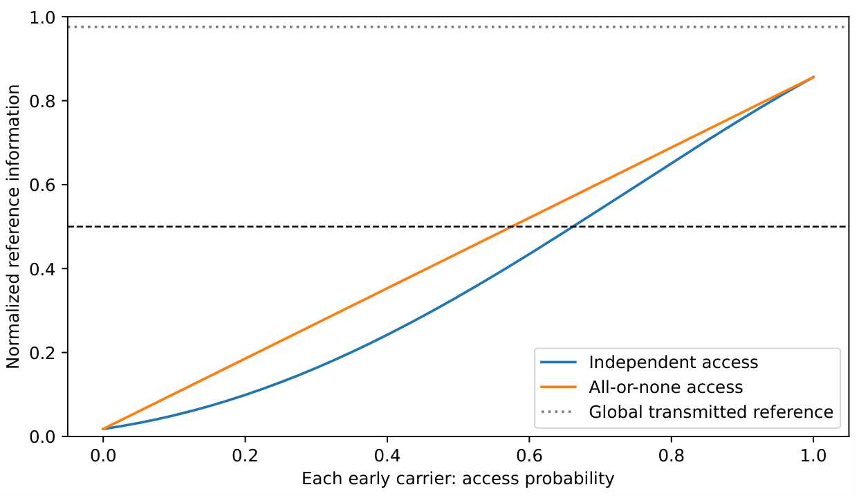
The source tables contain all subset combinations for each seed. The random-number, QR-phase, and register-ordering conventions were selected using four first-seed entropy pairs. The remaining 31 seeds and additional subset values provide further checks. No continuous scale was fitted to a target result. The registered causal calculation gives maximum passive-balance residual and no carrier or source data-processing violation. The mean response delay is . A separately coded exponential cavity recurrence and explicit subset contraction reproduce terminal carrier probabilities within and the decisive QEC supply within , using the stored propagated waveforms and source tables. This recurrence checks detector integration and information contraction. The upstream notebook additionally generates the source states, solves radial scattering, and propagates the packets. Its source-information values agree with the comparison tables within ; the maximum observer-probability difference across three propagation runs is . The controlled propagation comparison below uses this source-to-detector calculation. The block-entropy identity underlying Eq. (102) agrees with the subset sum to . Removing terminal cavity memory preserves the endpoint signs. Reference decorrelation gives zero mutual information without changing carrier energy.
5.3. From Gaussian Receiver Noise to a Recovery Certificate
Loss is not the only way a receiver can damage a carrier. A noisy rail can replace a lost excitation, or preserve its population while changing its coherence. To carry such effects into the diary task, we need the logical channel induced by a specified receiving instrument. The following reduction provides that connection for independent, identical Gaussian rails, including phase-sensitive dynamics. It uses the Gaussian channel on the actual non-Gaussian dual-rail input; it does not replace that input by a Gaussian state with the same covariance.
Let be the single-rail channel. After applying , the receiver coherently checks whether the total output photon number is one. It retains that two-dimensional sector without learning which rail is occupied, and replaces every other outcome by one orthogonal flag . The environment is initially independent of the full encoded source, including the early register and reference. This instrument defines the accessible output under discussion. A joint-parity check alone is insufficient when higher odd photon numbers occur.
Equal thermal-loss rails already give a depolarizing one-photon sector [77]; loss detection and residual logical errors are central to dual-rail cavity encodings [78]. The channel family combining flagged erasure with Pauli noise is also established [74,79]. Here we derive its weights for the wider phase-sensitive Gaussian class and connect them to the finite source tables.
Proposition 13
(Exact logical channel of a symmetric rail receiver). For independent identical parity-covariant CPTP rail channels, define
The specified one-photon instrument induces the exact channel
where , the other are the logical Pauli matrices, and
All weights are nonnegative, and acceptance p is independent of the logical input. For a zero-mean Gaussian rail channel, the additional identity
holds. In the Gaussian case, keeping accepted qubits and replacing erasures by gives deterministic Bell fidelity
The channel identity also holds on inputs entangled with an arbitrary reference.
Appendix H.12 proves the proposition and evaluates the six matrix elements directly from the Gaussian channel matrices. These are exact low-Fock matrix elements, with no truncation of the output state. The characteristic-function and Fock-representation methods are standard [80,81]. Equal rails and independent environments are essential: unequal rail losses can make the acceptance probability depend on the logical state.
For carrier j, use the weights of its physical channel and put . If the carrier environments are independent, the existing HP tables give the following all-trial bounds for a fixed early subset T:
The lower bound uses an admissible ideal-source decoder for each observed mask. Histories containing an undetected Pauli error still contribute to the deterministic score; dropping their nonnegative Bell overlap gives the bound. The upper bound follows because the noisy channel is a postprocessing of ideal erasure at the same . Independent flagged early access can be averaged as in Eq. (102). Noisy mutual information itself is generally not the old exact subset contraction, and the earlier numerical certificates cannot be reused at unchanged probabilities without evaluating the new channel.
A worked noisy-source certificate.
For independent identical thermal-loss rails with transmissivity and environment occupation , the exact reduction gives , , and . Applying Eqs. (113)–() to all 32 frozen source tables gives the uniform, outward-rounded certificates
These deterministic scores include every erasure and undetected-error outcome. The channel parameters specify an illustrative thermal-loss receiver; they are not inferred from the Schwarzschild temperature. The companion evaluates this example directly from the source tables.
What survival and fidelity leave undetermined.
Even within this Gaussian class, matching p and does not match every operational task. Two physically admissible rail channels in Appendix H.12 give the logical weights
with the same and . For an equally likely pair of opposite known-basis input states, the optimal binary discrimination probability, including erasures, is in every Pauli basis for . For it is in the X and Z bases and in the Y basis. Thus the apparent equivalence depends on which task is asked. The additional signed correlations , together with p, reconstruct the entire logical channel in this symmetric Gaussian class. This is an explicit calibration witness, not an additional numerical claim about the five-carrier source.
What a complete interface calibration leaves undetermined.
An erasure flag describes what this instrument discards. It does not prove that the discarded physical state has lost all reference information. Consider independent identical quantum-limited amplifier rails of gain , and compare them with pure-loss rails of transmissivity . Their complete one-photon-plus-erasure channels are identical. The amplifier, however, has a two-photon sector of probability . Its established cloning-sector structure [83,84] permits a trace-preserving extraction of one qubit with conditional Bell fidelity . Retaining that sector therefore increases an achievable all-trial score by . At , the original interface has optimal fidelity , while this enlarged interface attains ; pure loss has no two-photon sector to exploit. The refined receiver keeps the sector record, so it can also reproduce the original interface by discarding that sector.
The two examples separate insufficient calibration within a fixed interface from insufficient access despite complete calibration of that interface. The enlarged receiver requires additional coherent sector handling and a decoder; the amplifier also requires its pump resource. Its improvement is not an equal-resource comparison of amplifiers and attenuators, nor a claim of optimal recovery from every bosonic output. For a field-detector calculation, the same discipline applies: the prepared signal, bath state, accessible output mode and number check must be specified before the resulting Gaussian map supplies a diary-recovery certificate.
5.4. Fixed-Source Controls for Schwarzschild Propagation
Returning to the pure-loss collection model, the early-radiation comparison changes the observer’s available correlations while holding the late channel fixed. A complementary calculation holds the source and observer fixed and changes the propagation transfer function. This separates the quantitative contribution of the Schwarzschild radial potential from the dependence on early-radiation possession.
We compare the full complex transmission with a unit-transmission reference and with the magnitude-only diagnostic . The unit-transmission reference removes the radial potential’s transfer function while retaining the specified observer lapse and frequency convention. The magnitude-only diagnostic removes the transmission phase at fixed spectral attenuation; it is not assumed to represent a causal scattering problem. Each condition uses the same 32 source states, positive-frequency spectral normalization, source emission phases, aperture, efficiency, cavity parameters, and proper-time interval . The source phases are calibrated once using the baseline Schwarzschild calculation and are then frozen, including under numerical refinement. The emission schedule and incident normalization are identical across conditions.
Table 4.
Fixed-source propagation controls at the common deadline. is the mean terminal collection probability over the five late carriers; the two normalized reference-information columns are means over the 32 source states with no early radiation and with all early radiation, respectively. The fidelity ceiling is the largest no-early ceiling over those states, and the floor is the smallest full-early floor. Bounds are evaluated for each source state before taking these extrema, independently of the adjacent information means. The table uses the baseline settings. Fidelity ceilings are rounded upward and floors downward; the other columns use nearest rounding. The magnitude-only row is a phase diagnostic.
Table 4.
Fixed-source propagation controls at the common deadline. is the mean terminal collection probability over the five late carriers; the two normalized reference-information columns are means over the 32 source states with no early radiation and with all early radiation, respectively. The fidelity ceiling is the largest no-early ceiling over those states, and the floor is the smallest full-early floor. Bounds are evaluated for each source state before taking these extrema, independently of the adjacent information means. The table uses the baseline settings. Fidelity ceilings are rounded upward and floors downward; the other columns use nearest rounding. The magnitude-only row is a phase diagnostic.
| Transfer function | |||||
|---|---|---|---|---|---|
| Full Schwarzschild | 0.445132 | 0.018876 | 0.856854 | 0.357163 | 0.815597 |
| Unit transmission | 0.611494 | 0.050967 | 0.948735 | 0.427893 | 0.927764 |
| Magnitude only | 0.440029 | 0.018230 | 0.852872 | 0.355357 | 0.811059 |
The curvature potential changes the available information substantially in this specified task. Replacing its transfer function by unity increases the mean late-carrier collection probability from to and the uniform full-early fidelity floor from to . The no-early ceiling nevertheless remains below in the reference arm. Thus the early-access separation persists when the potential is removed, while its quantitative recovery bounds depend materially on Schwarzschild propagation.
Magnitude-only phase diagnostic.
The full and magnitude-only transfer functions have identical spectral transmission probabilities pointwise, and therefore the same integrated spectral transmission, . Nevertheless, retaining the complex phase increases the mean collection probability by and the mean full-early reference information by in the common window. The phase reshapes the arriving packets relative to the fixed receiving interval, changing access to their existing diary correlations. Thus the greybody transmission probability alone does not specify the collected reference information for this coherent preparation and finite receiver. The direction of the change is set by the emission schedule and observation interval.
Positive-frequency packets have nonzero pre-window tails. The receiver starts empty at zero under each condition. For the first packet, integration over gives incident energies , , and for the full, unit, and magnitude-only arms, respectively. These tails are not collected. The common finite spectral support retains of the normalized source packet’s energy. The information calculation uses the incident probabilities within the receiver’s operating window.
A joint refinement from 321 to 641 transmission nodes, from to time steps, and from 2401 to 4801 packet-quadrature points, together with tighter radial tolerances and extended radial boundaries, changes the terminal collection probabilities by at most , the statewise reference information by at most , and either fidelity bound by at most . The source phases remain frozen during this refinement. Every arm satisfies the passive energy balance and the statewise bound by the corresponding time-cut incident information. The notebook Schwarzschild_Propagation_Controls.ipynb generates these controls and displays the packetwise and statewise comparisons.
A causal comparison at matched spectral transmission and mean delay.
To isolate temporal reshaping within a causal propagation family, we cascade the original Schwarzschild transmission with either a lossless dispersive element or a matched pure delay. With dimensionless frequency , write the two transfer functions as
where and are fixed by the source packet’s center and spectral standard deviation before recovery is evaluated. For real x, exactly. Its pole lies in the lower half-plane under the inverse convention. A number-preserving, lossless resonator with routed output realizes this response in the quantum-envelope model. The cascade excludes back-propagation into the original scatterer; the added element changes the receiving path after Schwarzschild propagation.
The resonator’s dimensionless group-delay kernel is
where is the fixed incident packet’s spectral probability density on the numerical frequency interval. The baseline value corresponds to coordinate delay and observer proper-time delay . It is frozen during refinement; recomputing the weighted mean on the refined grid changes by . Matching this mean leaves the arrival distribution and detector-filtered peak free to differ.
The source tables, emission phases, observer lapse, collection efficiency, detector parameters, and proper-time window remain fixed. The downstream detector starts empty. The upstream resonator is initialized from the packet’s prehistory and can already be populated at window opening. Its stored energy remains inaccessible to the observer. The detector’s own cavity retains its original accessible status in Eq. (99). No peaks are realigned and no waveforms are renormalized within the window.
Table 5.
Causal propagation comparison at the common deadline, using the refined grid. The controlled matched-delay comparison is between the last two rows; the first gives the original Schwarzschild baseline. Spectral transmission is identical in all arms, with integrated value . Collection is averaged over five carriers and reference information over 32 fixed source states. The ceiling and floor are statewise extrema, evaluated before aggregation; they are not obtained by applying the bound formulas to the adjacent means. Fidelity ceilings are rounded upward and floors downward; the other columns use nearest rounding. These are numerical certificates, rather than calculations of exact optimal fidelity.
Table 5.
Causal propagation comparison at the common deadline, using the refined grid. The controlled matched-delay comparison is between the last two rows; the first gives the original Schwarzschild baseline. Spectral transmission is identical in all arms, with integrated value . Collection is averaged over five carriers and reference information over 32 fixed source states. The ceiling and floor are statewise extrema, evaluated before aggregation; they are not obtained by applying the bound formulas to the adjacent means. Fidelity ceilings are rounded upward and floors downward; the other columns use nearest rounding. These are numerical certificates, rather than calculations of exact optimal fidelity.
| Propagation arm | ||||
|---|---|---|---|---|
| Schwarzschild | 0.445132 | 0.856854 | 0.357163 | 0.815597 |
| Matched pure delay | 0.396946 | 0.816954 | 0.339101 | 0.771425 |
| Causal dispersive element | 0.381318 | 0.801127 | 0.334390 | 0.754658 |
Relative to matched delay, the dispersive arm lowers mean collection by and mean full-early reference information by . The information difference is negative for all 32 tested states, ranging from to . The full-early fidelity floor decreases by and the no-early ceiling by . Four carrier collection probabilities fall and the fifth rises, so the aggregate change includes a redistribution among carriers.
What spectral transmission leaves undetermined.
The causal dispersive and matched-delay arms preserve the same at every frequency and match the prescribed spectrum-weighted mean group delay. They nevertheless deliver different reference information to the same finite observer. In the tested preparation, the dispersive arm supplies less normalized full-early reference information before the deadline.
The reason is physical. Frequency-dependent phase reshapes a coherent packet relative to the detector’s response and operating interval. The finite-window measurement retains cross-frequency interference terms whose phase is absent from the transmission probability; one mean delay does not determine those terms. A lossless upstream element can therefore change which existing diary correlations become accessible in time.
This causal numerical comparison establishes a requirement for describing the specified recovery task: spectral attenuation and mean delay must be supplemented by the temporal response seen by the observer. The result concerns collected reference information ; retained transfer into memory additionally requires a receiving instrument satisfying the stated channel conditions.
Pointwise transmission probabilities agree within in floating-point arithmetic, with equality exact in the analytic model. Doubling the transmission and packet-quadrature grids and halving the time step changes collection by at most , reference information by , and fidelity bounds by across the three arms. Independent causal evolution of the upstream resonator agrees with the refined spectral output within in waveform amplitude. Energy accounting includes initial and terminal resonator storage and closes within . The computational supplement specifies the resonator parameters and delay rule. This comparison uses one declared resonator setting and the prepared coherent diary packets.
Scattering phase already has an established role in black-hole spectral physics; for example, it determines a renormalized density of states in Ref. [70]. Here the causal comparison connects temporal propagation to finite-window reference information and recovery certificates. The access-envelope calculation next addresses a complementary loss of descriptive information: even after individual collection probabilities are fixed, the joint pattern of available carriers can still change recovery. The envelopes give the full attainable range within their specified instrument family.
5.5. Controlled Collection into Finite Retained Memory
Information at the detector is useful only while it remains available. We now add a finite controlled catcher that stores the outgoing carriers and preserves their diary correlations after collection ends. For carrier j, write , , and . The original access probability in Eq. (99) is . To store the outgoing field, place a directed absorbing memory downstream of the detector port. In the phase-matched rotating frame, choose the predetermined coupling
It gives the exact stored amplitude and probability
The control follows the known temporal envelope, while the unknown logical rail remains coherent. Identical controls on the two rails implement a logical erasure channel of survival probability , including for an input entangled with the reference and the other carriers. Each carrier requires a qutrit memory: vacuum and the two one-excitation rail states. Directed coupling leaves the upstream cavity response unchanged. At the deadline, disconnecting the memory from the field gives lossless storage in this model.
Controlled absorption of prescribed single-photon temporal modes and the startup singularity of perfect absorption are established results [72]. The positive in Eq. (119) supplies a bounded approximation with an explicit error and resource budget. For the frozen cavity parameters,
The apparatus requires phase and timing calibration, predetermined complex coupling, a directed cascade, and storage isolation. These controls specify the receiving channel whose retained output is evaluated below.
Let denote the source-table contraction in Eq. (102), with late survival probabilities . The normalized retained information is exactly
Every survival mask selects the corresponding HP source marginal, so the branchwise recovery bounds apply directly to the stored state. With and , the 32 sources and all three propagation grids give the conservative certificates
The baseline computed extrema are approximately and . These evaluate the retained-memory task; the certificates above evaluate the original cavity-inclusive access task. Mean full-early retained information is , compared with for cavity-inclusive access. The ideal coherent output buffer differs from the finite memory by at most in normalized information, uniformly in source, time and early-access setting. Appendix L derives the channel and error bounds. The fidelity certificates optimize over deterministic decoders on the terminal registers; decoder execution has its own time budget.
The joint accessible inventory after rejected output is discarded is . Define . Exact differentiation gives
This bound remains valid when decreases. For the full-early source 2026082108, the computed effective rate decreases from approximately at to at ; the respective positive gaps are and . Every source in both early-access conditions has a decreasing pair on each of the three grids. Thus this specified catcher fails the nondecreasing-activation requirement of the fixed-clock, constant-kinetic-normalization strip benchmark. Retained information still increases. The numerical test addresses that benchmark; a time-dependent kinetic factor requires its own independent calibration.
5.6. A Receiving Channel for an Imperfect Collected Register
The catcher stores individual carriers. A second receiving architecture transfers the whole collected register, including whatever imperfect diary correlations it carries. The finite Jacobi receiver performs that transfer without first decoding the diary. Let be its arbitrary input state. Here E denotes the early radiation already available to the receiving observer and retained throughout the transfer; it is a trivial register when no early radiation is available. Encode each basis label of X at source site 0 and use the same links for every label. Sites are the designated durable memory. For capture probability p, tracing the residual source gives, up to a label-preserving memory isometry,
The transport flag is independent of . Consequently,
The second identity uses unrestricted deterministic decoding with an accessible transport flag. It gives an exact bridge from the collected state’s recovery task to the terminal memory’s task.
Write and . The infinite receiving benchmark has , so its retained information obeys
Its strip-compatible activation follows from the declared Hamiltonian, source initialization and target memory. Perfect logical decoding on a successful branch is unnecessary. For finite N, the probability and hazard certificates of Theorem 4 apply to the same label-independent channel on the prescribed interval.
The source boundary fixes the supply interpretation. If X is an admitted residual register in the observer’s accessible system, total accessible information stays at during transfer into designated storage. If X is outside that system, is an upstream input budget. It then describes source-to-receiver capture and is distinct from the instantaneous observer availability . In either case the terminal task is recovery from after the source is disconnected. For the HP construction , while the conditional quantity records the usefulness of late radiation together with early side information.
Five retained qutrits give . Each transport site requires 244 levels: 243 data labels and a separate transport-absence state. The all-erased five-carrier word is one of the data labels. Early radiation stays in its existing register. A front-end whose complete output code is the declared site-0 code avoids an instantaneous loading step; realizing the uniform exchange on this composite code requires collective, label-independent interactions and source isolation. The declared initialization and couplings select strip-compatible infinite dynamics; the finite receiver supplies certified operation over the chosen time interval. The positive-Hamiltonian implementation is specified alongside Eq. (A174).
5.7. Progressive Collection Followed by Recorded Register Capture
Quantum-buffer and repeater studies distinguish stored quality from availability and waiting time [75,76]; age-pattern distributions can also determine the performance of a later quantum task [91]. Here we compose those distinctions with the frozen HP source and propagated detector output to determine what a progressively collected, undecoded register can deliver before its acquisition deadline. A recorded collection front end makes admission time part of that receiving channel. For the detector output in Eq. (119), let and . Consider a rail-blind instrument that retains the logical qubit and records its accepted time, with Kraus density on the known temporal code
This is a specified temporal-to-buffer isometry with a readable time record, rather than separate rail-resolving photodetection. The accepted-time probability density is ; its integral is at most one, and an orthogonal failure outcome completes the instrument. The control is predetermined and identical on both rails. This recorded instrument and the coherent catcher have the same fixed-time survival probabilities; the temporal-to-buffer transfer and time record are additional apparatus operations, with their own resolution and error budget. Independent instruments give independent defective arrival times. The recorded instrument is a separate apparatus: increasing one-time survival probabilities alone do not identify a multi-time collection process. The finite numerical model uses piecewise-linear arrival CDFs through the saved time grid; a finite-bin implementation must specify its tie handling.
Stop collection on each run when the mth accepted late carrier arrives. Let H be this gate time and S the accepted subset, . For continuous arrival distributions, their joint density is
Thus . Freeze the collected register , keep early radiation E unchanged, and admit to the receiving source after routing duration . No diary decoder is applied during collection or admission. A recorded uniform transport channel subsequently delivers to durable memory with probability , where for . The gate, subset, and transport records remain available at readout.
Proposition 14
(Progressive register capture). For a fixed HP source s, write , with . Assume lossless buffering, routing, early storage, and terminal holding, and the label-independent recorded instruments specified above. Let be the available classical gate, subset, and transport record. The designated retained register is , and its normalized information is exactly
An attainable deterministic entanglement-recovery fidelity satisfies
If the receiving channel uses one common absolute-time Markov hazard , so that
then, almost everywhere,
Here is the supply in the designated post-gate receiving system; information still in the upstream buffer is accounted for separately.
Proof.
For each recorded , successful transport produces the unchanged state on , while failure leaves and an orthogonal memory-vacuum flag. The record probabilities are independent of . Orthogonality and therefore give a conditional information contribution , proving Eq. (130). On success apply a branch recovery decoder attaining Bell overlap at least ; on failure output a fixed qubit, whose Bell overlap is . Averaging includes every outcome and proves Eq. (131). For Eq. (132), differentiation gives and the admission boundary contributes zero, which proves Eq. (133). □
Each transport site requires levels: the collected logical labels and one transport-vacuum state. The subset record is classical; upstream carrier buffers and early radiation remain separate resources. Uniform collective exchange, routing, and source isolation are physical requirements. A recovery decoder acts after capture and has its own execution and readout budget. Imperfect front-end or storage channels must be included in their corresponding error budget.
A receiver initialized anew at instead has an age-dependent kernel . Equations (130) and (131) still hold, but a common-clock scalar law requires Eq. (132). For a finite receiver isolated at a preselected duration , replace its active age by and hold the resulting memory. The terminal certificate then uses the certified finite-receiver capture floor at that duration; it makes no global strip-membership claim.
The records and common clock are substantive conditions. For example, write and for Bell-state projectors. Equal recorded branches and each have normalized information ; forgetting their branch record reduces the mixture’s information by . Likewise, two equally weighted unit-information cohorts admitted at 0 and 1, each with reset hazard , have . Using the absolute-time rate in a scalar law would instead give . Thus resetting a receiver’s age cannot silently replace the common-clock hypothesis.
Frozen sources and the finite receiving chain.
We evaluate Eq. (131) using every source’s and all three supplied propagation refinements, with , , and the same , , chain used in Section 8.5. The largest link remains . The gate initializes the chain at , so this example uses the age-dependent cohort formula, not the common-clock scalar specialization.
Source isolation and lossless holding permit acquisition to end before readout. We preselect on the duration grid, independently of the source and gate outcome. Define
with for negative available duration and from Eq. (188). After that active duration the source link is disconnected and captured information is held until T. This prevents a long available interval from forcing continued interaction past the finite chain’s useful certified interval. The probability floor at the selected stopping duration is approximately . The table uses ideal source isolation; a finite switch contributes to the control-error budget in Eq. (A188).
Table 6.
Recorded progressive collection at fixed receiving-chain scale. Entries round downward after taking the minimum over all 32 sources and all three propagation refinements. Routing time ℓ is supplied; buffering, routing, early storage, and terminal holding are lossless.
Table 6.
Recorded progressive collection at fixed receiving-chain scale. Entries round downward after taking the minimum over all 32 sources and all three propagation refinements. Routing time ℓ is supplied; buffering, routing, early storage, and terminal holding are lossless.
| Gate m | Levels per site | |||
|---|---|---|---|---|
| 1 | 3 | |||
| 2 | 5 | |||
| 3 | 9 | |||
| 4 | 17 | |||
| 5 | 33 |
The two-carrier gate gives the largest lower certificate among the five count gates tested at each displayed routing time. It reaches a floor above with a loading interval and five local levels, using partial HP correlations directly. Waiting for a third carrier increases the correlations available on successful admission, but reduces the probability of reaching the gate before the deadline and leaves less time for capture. On the baseline grid at , gate probability falls from approximately for to for , while the certified captured-register probability falls from to . Under this schedule those costs outweigh the additional information. The column is an ideal routing benchmark. The nonzero columns budget routing duration without specifying a routing circuit or its error; the stated lossless channel remains an assumption. The recovery decoder acts after acquisition and its execution time is separate from T.
This is a receiving-register tradeoff, not a resource-equivalent improvement over the larger-code serial receiver. That receiver guarantees with 244 levels per site on its selected schedule, while the recorded gate introduces arrival records, conditional packing, and a smaller retained register. Moreover, unrestricted recovery from a continuing catcher at T cannot be worse than the gated terminal task. Its readable terminal mask can be supplemented with diary-independent virtual arrival times drawn from the accepted-time distributions conditional on arrival by T. Selecting the first m, discarding later carriers, and applying the receiving channel reproduces the gated output by CPTP post-processing. The gate therefore addresses delivery under a specified receiving-register constraint. Partial information in the frozen HP branches requires no binary-authorization approximation.
The companion evaluates the first-gate density within each saved time interval, splits intervals at routing and source-isolation boundaries, and compares quadrature orders. Sourcewise bounds are formed before their extrema are taken; averaging the source table first would answer a different question. The same recorded channel and branch coefficients determine the common-clock and age-dependent receiving comparisons.
5.8. A Finite Receiver with Switching and Storage Loss
The receiving task can also be completed by a controlled exchange that targets terminal recovery directly. Consider two sites, with X initialized in the source code and the memory empty. Every data label undergoes the same exchange,
The envelope is one until , then decreases smoothly as , with , and is zero from onward. Its pulse area is exactly , so the noiseless exchange transfers every label completely. This uses the exchange mechanism of Eq. (35); the control selects a terminal transfer rather than the modular trajectory. Appendix J.4 derives the resulting channel.
Let uniform excitation loss act at rate throughout the acquisition and switching interval , followed by storage for at rate . The memory’s transport-absence state records failure. The retained register therefore has the exact flagged channel in Eq. (125), with
Loss can remove the excitation during capture or storage; all such outcomes remain in the deterministic score. The early register E, when available, is protected during this additional receiving interval.
For the HP catcher inputs, gives . Equation (126) transports the existing certificates into the stored output:
These inequalities hold for every one of the 32 source states. The same channel preserves a verification separation:
The final decoder and reference comparison have their own execution times.
Storage loss supplies a contrasting outcome on the same receiver. Raising only its rate to gives and, for these HP inputs, the decoder-independent ceiling
Thus finite acquisition, a smooth switch, and nonzero loss can retain the access separation, while sufficiently severe storage loss prevents fidelity above one half. The appendix gives the corresponding storage-time bounds.
The full five-qutrit input has 243 data labels, requiring 244 levels per site. Initialization in that code, label-independent exchange, protected early memory, and the stated loss rates define this receiving experiment. A separate loading operation requires its own time and error budget. The total receiving and storage duration is after collection; it does not replace the collection window . The maximum link magnitude is below the allowed for the three-site comparison in the appendix. This comparison matches an available link bound; its source variance and physical separation are separate specifications.
Figure 3.
Recovery guarantees during storage in the two-site example. Acquisition lasts with loss rate ; storage loss is and the early register remains protected. The retained probability is . For full early access, the lower certificate guarantees before ; the upper certificate excludes from onward. The intervening interval is unresolved by these bounds. Every loss outcome enters the score; decoder and final readout durations are separate protocol resources.
Figure 3.
Recovery guarantees during storage in the two-site example. Acquisition lasts with loss rate ; storage loss is and the early register remains protected. The retained probability is . For full early access, the lower certificate guarantees before ; the upper certificate excludes from onward. The intervening interval is unresolved by these bounds. Every loss outcome enters the score; decoder and final readout durations are separate protocol resources.
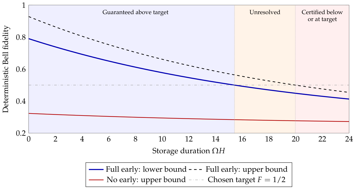
5.9. Access Correlations and What Marginal Collection Certifies
Knowing each carrier’s collection probability does not specify which carriers arrive together. The following comparison changes that joint structure while preserving every early carrier’s individual access probability. It asks whether two equally efficient collections, judged one carrier at a time, give the observer the same information.
For the designated state, independent early access crosses at . The root of the mean information curve is ; the 32 individual roots span –. Collective all-or-none access instead gives , whose mean-curve crossing is . Each early qubit has marginal access in both protocols. Their different boundaries expose information discarded by the marginal description.
We can determine the entire range permitted by those marginals. Keep the source and causal late detector fixed, and set
Here T denotes an early subset; distinguishes the observation deadline. An allowed access channel draws that subset with probabilities independently of the diary and late erasure events, keeps , and records the subset flag. Define
These finite linear programs optimize over all 32 early-erasure masks subject to the fixed marginals. The quantum source, flagged-erasure instrument family, and late detector are held fixed.
Proposition 15
(Sufficiency of a collection description). Let specify normalization and measured linear statistics of an accessible flagged collection law, and let h contain its subset-information values. If the feasible set contains a strictly positive distribution, these statistics determine the information value for every compatible law exactly when . With only individual collection probabilities specified, this requires to be affine in the membership indicators.
Equation (A97) proves the criterion. It gives a constructive meaning to a sufficient observer description: additional joint statistics supply rows of A, and determine the score once their span contains h. Until then, the access envelope measures the remaining ambiguity. The question is therefore which collection measurements determine recovery for the chosen encoding.
The lower bound is the least information compatible with the measured marginals; the upper bound is the greatest. If , every allowed access law has positive coherent information. If , none has positive coherent information. If , both signs are attainable. Certifying a sign therefore requires less information than determining the exact value: the interval can have nonzero width while lying entirely on one side of the boundary. These statements concern coherent information; deterministic recovery quality is separately bounded by Eq. (105).
For the mean table , the upper envelope first reaches one half at and the lower envelope reaches it at . Below the first value every allowed law has negative mean coherent information; above the second every law has positive mean coherent information. Between them the joint access law can determine the sign. These are optima of the mean table, not averages of individual optima. For individual states the first crossing spans –, and the last nonpositive boundary spans –.
Figure 4.
Sharp information envelope for the mean source-information table at fixed component early-access probability. The shaded set contains all values produced by the declared joint flagged early-erasure laws with the late detector fixed. The curves are extrema of the mean table, not means of sourcewise extrema. The lower panel resolves the region in which access correlations can determine the sign.
Figure 4.
Sharp information envelope for the mean source-information table at fixed component early-access probability. The shaded set contains all values produced by the declared joint flagged early-erasure laws with the late detector fixed. The curves are extrema of the mean table, not means of sourcewise extrema. The lower panel resolves the region in which access correlations can determine the sign.
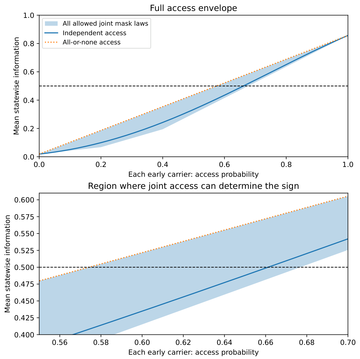
At common marginal , the mean-table interval is . A simple source-independent comparison makes the effect explicit. Keeping a uniformly chosen three-qubit subset gives across all seeds. Keeping all five with probability and none otherwise gives . Both protocols give every qubit the same access probability, yet their coherent-information signs are opposite for every fixed state. The envelope establishes when marginal measurements already certify a sign and when joint access measurements can change the conclusion. Early radiation alone has in the source construction; its value here resides in the additional correlations accessible jointly with late radiation.
The same calibration question for classical records.
The distinction also applies to records that can be copied. Work on quantum Darwinism already distinguishes redundant encoding from the consensus available under a specified distribution of environmental fragments [92]. The following example isolates the additional joint measurement needed to certify simultaneous correct readout.
Let a uniformly random classical bit X be copied into carriers , while contain blanks, following the informative/irrelevant-record construction of Ref. [93]. A source-independent assignment gives observers distinct carriers and their labels, with each observer receiving each carrier with probability . Their complete individual access channels are therefore fixed: each obtains bit of information about X and has optimal readout accuracy . They commit their answers before X is disclosed; every trial is scored.
Write q for the probability that both observers receive informative carriers. Without communication carrying information about X, their optimal probability of both answering correctly is
Uniform assignment over gives ; uniform assignment over gives . The resulting joint accuracies are and , despite identical individual channels and the same source’s uniform-fragment information curve. Measuring the joint validity flag—whether both collected carriers are informative—determines q and hence the score. It does not require reading X.
Allowing sufficient communication before commitment instead gives : the two protocols then score and 1, reversing their ranking. The actual pooled information, bits, also differs; it was never held fixed. Appendix H.13 proves these statements and the calibration repair. The example concerns access to existing classical records, rather than a new criterion of objectivity. Agreement alone is not correctness: two observers can always agree by outputting a fixed bit. Nor does redundant classical readout certify the stronger quantum-reference correlations constrained in Section 8.3.
5.10. Recovery Guarantees Under Uncertain Joint Collection
The branchwise certificate lets us ask whether the recovery separation survives uncertainty about losses themselves. Enlarge the collection family to all source-independent flagged late-erasure laws with the five registered late marginals, while keeping the source and deadline fixed. This family includes the original independent detector and also correlated collection instruments. Linear optimization of the branch certificates gives, for every frozen source,
The separation therefore survives arbitrary dependence among these late losses. When both observers use the same late law, a paired certificate guarantees an advantage of at least for full early access.
Partial early access exposes what the marginal description omits. Fix all ten early and late collection probabilities, with early marginals , and permit dependence among all ten flags. One common source-independent law then has for every frozen source. Its seven nonzero mask weights are explicit, and its worst-source upper certificate attains the numerically sharp value of the common-law certificate optimization. Adding the joint condition
instead gives uniformly over the resulting law class, where and count collected late and early carriers. Measuring this joint collection frequency excludes adverse access laws that the component probabilities alone permit, and supplies a uniform recovery guarantee. Appendix H.6 gives the optimization, attaining obstruction and a simpler total-count certificate with an explicit flag-readout model.
5.11. Access Patterns at Fixed Collection Size
The preceding comparisons match individual collection probabilities while allowing different distributions of the number collected. Fixing that number provides a further test of what the observer’s access description must contain. We compare two protocols that each collect exactly three of eight sites: uniform selection among the eight contiguous windows on a periodic boundary, and uniform selection among all three-site subsets. Every site is included with probability in both protocols. Their difference is which sites are available together.
The source is a logical qubit maximally entangled with reference Q and encoded into eight boundary qubits by a finite binary multiscale entanglement renormalization ansatz (MERA) [71]. Seven isometries and six disentanglers define the bond-dimension-two encoding. We evaluate 64 independent random, unoptimized encodings. Each is paired with a tree that keeps the same isometries and replaces all disentanglers with identities; 64 independent Haar isometries provide a comparison at the same input and output dimensions. The construction and sampling rules are specified in Appendix C.1.
For a collected subset S, define its available reference information by
where contains the eight cyclic triples and bit. The subset is chosen independently of the input and recorded in an accessible flag. The averages therefore equal the normalized reference information of the respective flagged collection channels. They measure the supply available to a receiving instrument.
Equal collection size and efficiency do not determine acquired information.
Both protocols collect three sites, and each site is collected equally often. Contiguous access nevertheless acquires more reference information in all 64 sampled MERA encodings.
| Encoding ensemble | Contiguous | Uniform subsets | Gap |
| MERA | |||
| Paired tree | |||
| Independent Haar |
Entries are means over 64 encodings in each ensemble. The mean MERA gap is , with approximate bootstrap interval .
The disentanglers increase the gap by on average, with interval . Amplification occurs in 59 pairs and attenuation in five. At the same time, the disentanglers lower acquisition under both protocols: the mean changes relative to the paired trees are for contiguous access and for uniform access. Greater separation between access patterns can therefore accompany less information acquired by both observers.
The paired intervention identifies a change in how the encoding distributes information across accessible subsets. With , its positive mean records a larger contiguous-access preference. In three of the 64 pairs, removing the disentanglers reverses the preferred collection protocol from contiguous to uniform access. The independent Haar ensemble has mean gap , with interval ; its permutation symmetry gives zero expected gap. The intervals quantify Monte Carlo uncertainty over the specified encoding distributions, with each encoding as the sampling unit.
These results supply fixed-size witnesses of the marginal-sufficiency criterion in Eq. (A97). On the domain of three-site subsets, the two access laws have the same normalization and membership constraints, yet different information values. Even the full distribution of the number collected, together with every individual collection probability, leaves this observer information undetermined. The joint collection pattern must be evaluated against the encoding.
The access budget can also reverse the preference without changing the encoding. Purity of the joint reference–boundary state gives
because the complementary ensembles are precisely the cyclic five-site windows and all five-site subsets. The same disentanglers that lower both three-site acquisition means raise both complementary five-site means. This reversal follows exactly from the same states. The following code construction gives an exact recovery-fidelity counterpart to the dependence on joint access.
5.12. An Exact Erasure-Code Comparison and the Transfer Interface
An independent source comparison uses the code with a maximally entangled diary reference. Every three-carrier subset reconstructs the diary and every subset of at most two carriers is reference-decorrelated. This threshold structure is the quantum-secret-sharing relation developed in Ref. [41]. Consequently , where K is the number of surviving carriers. Homogeneous independent survival gives
The actual heterogeneous terminal probabilities are
The same propagation and cavity then give and . Thus a second source architecture separates transmitted reference information from observer supply.
Keeping these five marginals fixed while allowing arbitrary joint flagged erasures yields the sharp interval
Writing , the elementary survivor-count bounds are . Explicit access distributions attain both endpoints for the present marginals; Appendix H records the witnesses. They are alternative correlated erasure instruments sharing the five individual efficiencies of the cavity calculation. The sharp interval shows how much the joint collection structure can matter even for an exact code.
For this code, the information interval also gives an exact recovery-fidelity interval. The mask flag tells the decoder which shares remain. Three or more shares permit perfect recovery; at most two carry no reference information and give optimal Bell overlap . Thus, with ,
Both endpoints are attained at the same five individual efficiencies. Appendix H proves the branchwise optimization and records its control assumptions. The interval measures a physical uncertainty left by component calibration: it spans markedly different deterministic recovery quality even though every carrier has the same stated probability of collection.
The access pattern must fit the encoding.
The exact code envelope in Eq. (150) quantifies the recovery variation left open by individual collection efficiencies. Comparing encodings reveals a further consequence: the preferred joint collection pattern can reverse.
At common marginal access , uniformly retaining exactly three QEC shares gives , whereas all-or-none retention gives . For the HP early-access comparison, with the late detector fixed, exactly-three access gives and all-or-none access gives for every tested source state. The QEC values are exact code consequences; the HP inequalities hold across the 32 source calculations.
The same mask laws favor different encodings. A useful collection pattern preserves the combinations of carriers that carry the particular source’s diary correlations. Individual detector efficiency cannot identify that pattern.
The collected state is also the input to a physical receiving process. For an HP output, the carrier flags identify subsets with generally partial diary information. Section 5.5 follows those carriers into retained memory; Section 5.6 derives an exact acquisition law for uniform transport of the complete collected register. Joint access therefore determines both the state offered to a receiver and the evidence an observer can obtain about preservation.
Receiving noise can reverse the preferred access pattern.
The encoding can also remain fixed while the preferred protocol changes. Use the same five installed receivers, each with a source site and a memory site supporting vacuum and two coherent qubit labels. An activated receiver implements a flagged erasure channel with survival probability s; survival events are independent conditional on the activation mask. The mask is chosen independently of the diary and is available to the observer. Unactivated shares remain outside the terminal observer system. The finite pulse and uniform loss channel of Section 5.8 provide one realization, with for the active receiver’s total loss exposure D.
Proposition 16
(Noise-dependent ordering of receiver controls). For the five-share code, protocol A activates all five receivers with probability and none otherwise. Protocol B activates a uniformly chosen triple. Both activate three receivers on average and give every share terminal survival probability . Their authorized-set probabilities and optimal deterministic recovery fidelities are
The difference factors as
Thus B is better for , whereas A is better for ; they agree at and .
Exactly-three activation guarantees the required shares when transfer is ideal, but any subsequent share loss defeats that branch. All-five activation supplies redundancy whenever it occurs. Increasing receiver loss can therefore reverse the ordering without changing the encoding, installed hardware, or equality of individual terminal efficiencies. For example,
| Per-active-receiver survival | ||
Both controls use the same duration, per-active-receiver loss, coupling cap, and expected integrated squared coupling. The installed apparatus permits five simultaneous active links; A uses that peak, while B uses three. Their selector entropies also differ. Appendix H.9 gives the derivation and resource accounting. Every activation and loss outcome contributes to the reported fidelity. The construction applies the established code threshold to finite noisy receiving controls.
5.13. Access and Verification of Preserved Reference Correlations
What can an observer conclude when recovery fails? In the five-carrier construction, collecting at most two carriers gives identical evidence under diary preservation and reference erasure, even with access to the reference. The observer’s failure therefore does not reveal which global process occurred. To make the comparison precise, let V be the five-qubit encoding isometry and compare
Here preserves the diary in the encoded radiation, whereas replaces its input and erases its reference correlations from that radiation. A reference-assisted verification experiment compares the hypotheses using a Bell input . The diary decoder acts only on the collected registers; the verifier subsequently measures the retained output jointly with Q.
Proposition 17
(Access-dependent verification). For every subset S of at most two code shares, the reduced channels and coincide, including all ancillary extensions. Suppose a source-independent collection law supplies an accessible mask flag and has authorized probability . Transfer the complete collected register through a label-independent flagged capture channel with probability p, the same for every mask and both hypotheses. Then the optimal equal-prior success probability for joint reference–memory verification and the preserving channel’s optimal deterministic Bell recovery fidelity are
The recovery decoder has no access to Q.
The proof in Appendix H.10 uses exact erasure correction and the orthogonality of the collection and capture records. On an authorized captured branch, recovery gives a Bell pair under and the maximally mixed two-qubit state under . Their trace distance is . Every other branch has identical reference–memory states under the two hypotheses.
At common marginal collection probability , the sharp authorization range is . Uniform three-share collection attains the upper endpoint; mixing uniform two-share collection with full collection in proportions and attains the lower endpoint. Thus the same five individual efficiencies and the same receiver permit the exact interval
The joint collection pattern changes the evidence that reaches the verifier. Under an unauthorized access rule, preservation and reference erasure are the same experimental object. With sufficient carriers, their distinction becomes measurable through comparison with the reference. That reference access is essential: for the Bell input, the radiation marginal alone is under both hypotheses, even at full collection.
The HP calculation asks the same verification question for the propagated diary and its retained output. Here an attainable verification score with early radiation exceeds a universal upper bound without it. The unauthorized-code comparison above instead gives exact channel equality.
Corollary 10
(Verification separation for the retained HP output). For each of the 32 HP sources, compare the declared source with the same source preceded by replacement of the diary by . Prepare a Bell input and use the controlled catcher at the receiving deadline specified in Section 5.5. Let X include the retained registers and their accessible collection records. The two reference–output states are
Their X marginals coincide. With equal prior probabilities, optimal joint reference–output discrimination satisfies
The reference is available only to the final verifier; the recovery decoder acts on X alone.
The lower bound follows by applying a certified recovery decoder and testing its output jointly with Q against the Bell state. The upper bound applies to every joint reference–memory measurement and follows from the no-early information ceiling. Appendix H.11 gives both derivations. Thus the same HP source and late receiving device produce a certified separation in the evidence available about preserved reference correlations. These are terminal-state discrimination bounds; the final reference comparison has its own readout time.
5.14. Observer-Channel Ordering
The comparisons so far change access to a fixed source. When one observer’s channel can be obtained by degrading another’s, we can order their reference information directly by data processing.
Proposition 18
(Ordering under observer-channel degradation). Suppose that, at proper time τ, observer j’s memory channel is a CPTP post-processing of observer i’s channel,
Then
Proof.
Apply data processing to and normalize by . □
Equation (159) supports controlled comparisons of nested apertures, passbands, or post-processing chains when the degradation map is established.
5.15. Trajectory, Receiving Time, and Control Resources
The ordering of two receivers also depends on what is held fixed along their trajectories. Communication between freely falling and hovering observers, including dual-rail reference correlations, has an established literature [85]. Wavepacket compression and finite-bandwidth matching are likewise established effects [86]. Here we ask a more specific question: how does a finite receiving interval change recovery of the same encoded diary?
For this comparison we stipulate an outgoing chiral Markov channel carrying the transmitted envelopes of Section 5.1. Its vacuum input, temporal normalization, and passive cavity define an effective receiving model. This is a conditional channel construction; a time warp of the asymptotic envelopes does not derive the coupling of a localized detector to the full Schwarzschild field.
Both receivers start at at the same event, with empty cavities and the full early register E. One remains static; the other follows an ingoing radial geodesic of conserved energy per unit rest mass equal to one. The latter is already moving inward at , rather than being released from rest there. They use the same 32 frozen source states, the same independent dual rails, , , and . Retained systems comprise the detector output accumulated by the endpoint and the current cavity mode. The reflected port remains inaccessible. Early storage and subsequent decoding are ideal; the receiving deadline does not include final-decoder execution time.
Let be the static receiver’s proper-time label for the outgoing wavefront met by the infaller at proper time , with . Writing , the stipulated moving envelope is
The square-root factor preserves pulse norm over matching wavefront intervals and the Markov field commutator. Identical action on the two rails therefore gives an input-independent erasure probability for each carrier. Appendix H.15 derives the trajectory, cavity evolution, and recovery certificates.
Stopping at gives
During this proper lifetime the infaller encounters a larger portion of the outgoing stream than the static receiver. Applying the resolved-mask bounds of Eq. (106) gives, for every frozen source,
These are numerically evaluated bounds on optimal deterministic Bell fidelity, with every collection outcome included. They are not measured fidelities or statistical confidence intervals.
Table 7.
Three comparisons within the same effective receiving model, at the infaller’s endpoint. The first row matches proper duration; the second matches the encountered stream; the third adds a specified control.
Table 7.
Three comparisons within the same effective receiving model, at the infaller’s endpoint. The first row matches proper duration; the second matches the encountered stream; the third adds a specified control.
| Comparison | Consequence |
|---|---|
| Same proper duration and fixed cavity parameters | The infalling lower bound exceeds the static upper bound by more than across all 32 sources. |
| Same outgoing wavefront interval and fixed cavity parameters | Static collection probabilities dominate componentwise. Static optimal recovery is therefore no worse; the bounds do not establish a strict fidelity separation. |
| Same outgoing wavefront interval with adapted cavity parameters | Scaling both port rates and resonance by reproduces the static erasure channel exactly, at increased peak rates and frequency. |
The adaptive identity is a time-reparametrized input-output control, consistent with established tunable-capture methods [72]. Along the tested trajectory, increases from to ; the final required linewidth is . Frequency tracking alone does not supply this control. The integrated coupling dose agrees over matched wavefront intervals, while the peak coupling requirement changes.
Stopping earlier at gives the same qualitative comparison and a strict equal-proper-time separation . Both endpoints remain outside the horizon. The matched resources are the stated cavity parameters and duration or stream interval. They do not include equal hovering energy, trajectory preparation, aperture geometry, or the cost of additional controls. Consequently, Eq. (162) is a concrete recovery comparison for a declared channel, rather than a universal ranking of static and infalling observers.
5.16. Detector Response and Reference-Information Transfer
The following wavepacket construction realizes the receiving step on a diary-bearing branch. It specifies the capture operation, its event record, and the resulting information-transfer hazard.
For an Unruh–DeWitt coupling with switching , the finite-time response along the detector worldline is [22]
where W is the field two-point function in the specified state and is the detector gap. The coupling strength and detector matrix element convert this response into the leading-order excitation probability. The worldline, switching, and field state determine the response; correlation with Q identifies its diary-bearing component.
As a one-wavepacket benchmark, let be a selected outgoing packet inside the protocol support and let be a retained memory mode. On the branch in which carries the diary data, a number-preserving capture interaction implements
with orthogonal records for capture and noncapture. Tracing the record reproduces the transfer channel in Eq. (26). On the captured branch the purification is moved into memory; it is not copied. Equations (35)–(37) give the corresponding repeated-interaction unitary, while Eq. (33) shows that the capture record learns the event without learning the diary.
Suppose independently resolved capture opportunities form a Poisson process of intensity and a reference-correlated opportunity is retained with conditional probability . Over an interval with approximately constant parameters, the probability of no successful capture is
Combining this survival factor with Eq. (38) gives the continuous hazard
Here is calibrated from detector response, while contains mode overlap, transfer efficiency, and reference sensitivity. Their product gives the information-transfer hazard when successful events implement the flagged reference-transfer step. Detector calibration and branch-fidelity measurement therefore fix complementary parts of the acquisition model.
5.17. Observer-Dependent Entropy
Observer-dependent retrieved entropy is the reference-correlation quantity defined in Eq. (6). Its instantaneous ceiling is , the diary information within the observer’s causal collection and memory channel. The remaining transfer gap is therefore .
5.18. Retrieval Law (Instantiation)
For the flagged-transfer family derived in Section 4, the observer instantiation is
5.19. Inherited Speed-Limit Constraint
Observer retrieval trajectories inherit the activation constraint in Section 4.5. Within its strip-holomorphic class, the hyperbolic tangent is the equality activation profile; integrating the transfer law gives the retained trajectory . Observer protocols change the causal supply , the kinetic factor , the calibrated activation clock, and therefore the composite hazard . Distinct proper-time signatures follow when those calibrated inputs differ.
6. Quantum Information Correlations and Testable Predictions
How would the diary information retained in memory appear in a correlation measurement? Correlation imaging tests a proposed map between these quantities. After independent calibration, the map must predict held-out correlation surfaces from the proper-time retrieval trajectory and distinguish those predictions from matched alternatives.
Controlled changes to the observer protocol act on the measurement through the following dependency chain:
Activation enters the primary observation model through the transfer law and the resulting retrieval trajectory.
The retrieval law in Eq. (167) constrains the latent reference-information trajectory. A measurement model is still required to relate that trajectory to radiation observables. We consider two diagnostics: the order- Rényi entropy of the selected subsystem and the second-order correlation function . Neither observable equals without an explicit state and detector map.
The prospective protocol first calibrates the baseline correlation parameters and estimates supply independently. The retrieval fit then determines the composite hazard from the latent trajectory. The test is whether these calibrated dynamics predict new correlation surfaces under held-out conditions.
6.1. Rényi Entropy and Second-Order Correlation Functions
In analog systems, controlled changes in flow configuration and detection geometry provide distinct protocols for comparing observer access.
For any subsystem A, the Rényi entropy is
with . Equation (169) arises by analytically continuing the integer-order moments (the replica trick); for a field-theoretic derivation see Casini, Huerta, and Myers [24]. Larger gives greater weight to the largest eigenvalues of . Relating changes in to the observer-dependent delay requires a specified state evolution and observation protocol. Here functions as a theoretical purity diagnostic, while the directly modeled analog observable below is , accessible through density–density correlation measurements in BEC analog systems [23].
To project the retrieval dynamics into a measurable correlation surface, let
Times are measured relative to the onset-aligned analysis window, with after baseline alignment. Let be the decorrelation time measured in the no-retrieval baseline. Define the connected excess correlation . A modeled suppressive envelope is
where and are fixed by baseline data. An independent reference-tagged calibration determines the sensitivity and tests whether the factors describe the selected platform’s response. For an observation-level fit, may instead be profiled as a common nuisance parameter. Equation (170) defines a candidate observation map: its separable structure can be tested from the correlation surface, while its interpretation in terms of retained reference information requires the tagged calibration. For positive baseline amplitude, the map is monotone in each and carries certified degraded-channel ordering into the projected suppression envelope.
On the constant-supply, constant- extremal benchmark, Eq. (67) gives
The tanh activation reaches the correlation surface through the derived retrieval trajectory.
The non-retrieval null sets and leaves the symmetric exponential baseline. Matched thermal, diffusive, and generic-saturation alternatives are then compared against the full protocol-conditioned surface.
The prospective correlation analysis uses nonlinear least squares on ensemble realizations consistent with the declared observer constraints.
Within this forward model, captures decay-modulated suppression associated with observer-indexed access, while tracks the spectrum of the independently measured subsystem state.
Controlled comparisons among observer protocols test the projected final link in Eq. (168). Independent activation measurements and reference-tagged memory close the preceding links.
6.2. Activation, Dose, and Held-Out Prediction
The prospective Tier 1 experiment separates calibration from prediction. Baseline data fix and , while the selected state and collection protocol supply . A separate detector calibration fixes or the activation observable. Retrieval data are then divided into calibration and held-out conditions to test the relations among these independently identified quantities.
For a baseline-normalized, delay-window-reduced envelope, the extremal constant-supply benchmark is
where is Eq. (67). With and calibrated, and with fixed by an external tagged condition, the onset scale is the remaining trajectory parameter. When is not fixed in advance, it is profiled as a nuisance parameter and the held-out surface remains untouched until prediction.
A nonlinear least-squares estimator minimizes
When is fixed by external tagged calibration, this is a one-parameter minimization over .
The modular speed limit is tested on an independently calibrated activation trace through
For an affine clock on the equality branch, . Because differentiation becomes ill-conditioned near saturation, the registered test window is restricted to , with smoothing, derivative estimation, and uncertainty propagation fixed before evaluation.
The checkpoint form in Eq. (64) gives a derivative-free activation test. Every registered pair must satisfy that envelope using the independently calibrated clock difference . Exact contact for one distinct pair forces the complete tanh equality branch within the analytic class. The accumulated quantity in Eq. (65) measures subextremal activation delay and must compose additively across adjacent acquisition windows. Under affine calibration, measured activation thresholds additionally test Eq. (66). These pairwise diagnostics remain available when the nominal onset time is uncertain.
The transfer law yields a second diagnostic. Define
Under the extremal constant-, constant- benchmark, Eq. (68) predicts that is linear in . Sequential capture windows must also compose additively in .
The non-retrieval null sets . Thermal, diffusive, generic-saturation, and non-gap alternatives are matched in parameter count. Calibration data determine the model parameters; a separate protocol or bandwidth condition tests the predicted , dose, and full surface.
The registered analysis requires (i) on the evaluation window, (ii) nonnegative and sufficiently smooth , (iii) independent estimates of the quantities placed in the denominator of Eqs. (56), (173), and (174), (iv) and , and (v) .
Calibration, uncertainty propagation, and held-out correlation prediction are specified by this prospective Tier 1 protocol. Varying detector bandwidth tests the onset scaling while keeping the analog background and analysis protocol fixed.
7. Experimental Signatures and Measurement Conditions
The experimental program follows the diary from collection into memory. Programmable receivers test whether matched component efficiency determines recovery, whether the collected information survives storage, and how to divide a fixed deadline between collection and transfer. BEC analogues test propagation, field correlations and receiving interventions through an observation map. Each comparison identifies the resource held fixed and the resource changed, so the measured contrast can be traced to a physical intervention.
A measurement of the probes must be sensitive to the diary correlation if it is to test retrieval. Two probe outputs can have the same complete state while carrying either two bits or zero bits of mutual information with the chosen diary reference Q (Appendix H.7). This provides a decisive control: preserve the probe marginal while changing its reference correlation, then test whether the proposed readout detects the change. Joint reference–memory measurements resolve that contrast and quantify retained acquisition. Direct tests of the activation envelope and terminal-dose criterion additionally specify supply and receiving dynamics independently. The BEC correlation program tests its observation map through controlled interventions and connects that map to diary retrieval through the reference-sensitive calibration.
7.1. Joint access, capture and verification at matched efficiency
The exact code of Section 5.12 also supplies a compact prospective quantum-processor test. Prepare the reference-entangled five-carrier source and independently choose either a uniformly random three-carrier mask or an all-five/none mask with probabilities . Realize discarded shares by tracing them out, resetting them without keeping an accessible record, or routing them to inaccessible registers. Deliver the mask flag to the decoder. Each carrier has survival probability under both laws, while ideal deterministic Bell fidelities are respectively one and .
An implementation must register its recovery circuits and resource budget before evaluation. One explicit library contains a recovery circuit for each three-share subset, the inverse encoder for all-five access, and a fixed output for no access. Both protocols use the same allowed library and a budget sufficient for its largest circuit. Predicted measured fidelity is then the weighted sum of calibrated branch scores. All shots enter the score; postselecting successful branches would conceal the deterministic difference. Source preparation, empirical marginals, flag reliability, and circuit errors must be checked before attributing the contrast to access architecture. Quantum-processor HP recovery and horizon-scrambling experiments provide relevant platform precedents [43,47]. This prospective test complements the BEC routes with a directly reference-scored recovery task.
Uniform capture of the collected register adds an independently calibrated probability p. For the preserving code, let q be the frequency of authorized masks with at least three surviving shares. The retained state then supports
where the second score is the equal-prior discrimination task of Section 5.13. The verifier compares the preserving encoder with encoded maximally mixed replacement, using joint reference–memory readout after storage. The reference remains unavailable to the recovery decoder. The uniformly random three-share protocol has ; all-five/none access has . Their fidelity difference is , and their verification-success difference is , despite identical component efficiencies. Restricted outputs containing at most two shares are identical under the two source channels. Additional joint access therefore changes both the attainable recovery and the evidence available about preservation.
The capture flag and collection mask must both be retained, and their calibration must establish input-independent capture. Varying p at fixed mask law tests the predicted affine dependence; varying the mask law at fixed p tests the joint-access contribution. Measured branch errors enter the same all-trial score as the ideal predictions. A verification completed by a deadline must additionally budget the final joint measurement.
Independent share erasure supplies a further intervention. After applying either collection law, let each collected share survive with the same independently calibrated probability s, retaining its erasure flag. The authorized-mask probabilities become and . Both protocols have terminal carrier inclusion probability and mean surviving count , yet their ordering reverses at : all-five/none access is better below this value, and uniform three-share access is better above it. Substitution into Eq. (175) predicts both measured scores at fixed capture probability. Recording joint survival tests the mechanism that individual survival calibration leaves unresolved.
7.2. A Programmable Test of Modular Acquisition
The finite receiver provides a direct test of reference-information transfer. Prepare a diary label maximally entangled with an untouched reference at the source site, initialize the receiver sites in vacuum, and independently calibrate the constant couplings in Section 4.7. The source state and Hamiltonian then fix the full predicted acquisition curve. Receiver size, acquisition deadline and loss tolerance are set before collecting the test traces.
At each deadline, disconnect the source and read the receiver. Joint reference–memory tomography estimates the retained mutual information; a coherent label decoder and vacuum flag give an independent erasure-channel score. Agreement between the two checks the assumed transfer sectors. The measured logarithmic gap derivative supplies the normalized activation only where the residual gap is resolved. A small retrieval error by itself leaves the derivative undetermined, so activation is compared with its own bound and measurement uncertainty.
Changing chain length tests the truncation certificate. Preparation dependence requires a three-way comparison: the centered source with its original partition, a translated preparation with that partition held fixed, and the translated preparation with its matched residual-source projector and complementary memory readout. The translated formula in Appendix I uses the last of these. Preparing translated coefficients in the original chain alone changes the initial occupation of its memory sites and does not implement that formula. A matched-projector implementation must specify the readout and isolation controls; an alternative chain built from the translated cyclic state requires its own couplings and truncation certificate. Initialization, coupling, switching and readout errors enter the respective resource budgets.
After disconnection at the deadline, the remaining question is whether the receiver keeps the diary correlation it acquired. Comparing reference correlation immediately after acquisition and after a specified storage interval separates transfer accuracy from retention.
Together, these measurements test the simulator’s stated Hamiltonian and channel. The controlled catcher of Section 5.5 extends the test to a traveling pulse, while the imperfect-input construction of Section 5.6 examines the interface between collection and subsequent acquisition.
7.3. Temporary Access, Retained Correlation and Imperfect Inputs
For a traveling pulse, the experiment must distinguish information temporarily present in the cavity from information retained in memory. Prepare a reference-tagged pulse and calibrate the cavity response and predetermined capture control independently of the unknown logical label. Measure cavity occupation , detector-port dose and stored probability on matched ensembles. The controlled catcher predicts and . Disconnect its memory at the chosen deadline and measure both stored population and reference correlation over a storage interval. A population-preserving dephasing control provides the decisive contrast: unchanged occupation can coexist with degraded diary coherence. Joint reference–memory tomography distinguishes coherent retention from energy storage, while the cavity trace tests temporary availability and leakage.
A single-qubit control gives the coherence test a quantitative target. The two-site pulse of Section 5.8 then requires only three levels at each site: transport absence and two logical labels. Prepare a Bell pair between the transported qubit and its retained reference, capture with input-independent probability p, and apply population-preserving dephasing whose independently measured coherence factor is . On a failed capture, output a fixed qubit state. Including every trial in the readout, the Bell overlap is . Changing v leaves the stored population unchanged while changing its reference correlation. This control tests the difference between storing an excitation and retaining a quantum diary before the full propagated-source experiment is attempted. The combined dephasing-and-erasure channel has established antecedents [74]. At the worked survival probability , coherent retention () gives , while complete dephasing () gives at unchanged capture probability. These are predictions for the reference-entangled qubit control.
A small three-register experiment can test the imperfect-input identity without implementing the full Hawking source. Prepare a calibrated correlated state , retain E at the receiver, and uniformly capture X with independently measured probability p. Joint tomography at several values of p tests
Varying the preparation changes the conditional information independently of the capture law. For example, a three-qubit GHZ preparation gives and in bits, hence the prediction . Dephasing that preparation in the computational basis preserves its marginal but removes the conditional contribution, giving a constant value of one. A Bell pair on with independent E instead gives . These controls distinguish side information, transported correlations and capture probability within the same apparatus. Every transport failure remains in the output state as a distinguishable flag.
7.4. Allocating a Fixed Acquisition Deadline
For delivery to a separate final register through the specified serial receiver, the collection cutoff is a controllable design variable. Keep the source family, catcher, receiving couplings, and total duration fixed; vary only the time assigned to collection and subsequent capture. If the catcher itself is the final memory, the continued-collection comparison in Section 8.5 supplies the appropriate control. Section 8.5 supplies a concrete target: at total duration , the tested split raises the worst-source certified Bell-fidelity lower bound from for to . The cutoff is selected using calibration data and evaluated on held-out runs. The measured acquisition probability and branch recovery scores determine the experimental comparison; the calculated lower-bound improvement supplies a certificate target rather than an assumed value of measured optimal fidelity. Storage begins at the common deadline, with the final readout budget declared separately.
A source-limited outcome improves when extra collection time contributes more than the capture time it removes. A transfer-limited outcome favors earlier isolation. The marginal-gain condition in Section 8.5 predicts the transition between these regimes and makes the allocation test more informative than comparing longer and shorter total runs.
7.5. BEC Correlation Surfaces and Controlled Interventions
For the BEC program, the central observable is the two-point function reconstructed from density correlations or equivalent detector outputs. The candidate map in Eq. (170) assigns a separable suppression factor to each time argument. Flow and horizon configuration, detector switching and sampling, spectral response, and normalization across repeated condensate realizations are independently controlled. Their variation tests how a changed source or receiving protocol changes the measured surface.
A BEC test begins with the observation map and the controls that can change the measured surface. Tier 0A identifies archives with sufficient timing, calibration and joint availability records; Tier 0B compares physical and analysis operators on those records. These comparisons guide the choice of a prospective Tier 1 intervention and a held-out prediction condition. Appendix K gives the archive requirements and supporting diagnostics.
Equation (170) supplies a direct structural test before fitting an activation trajectory. For , define the baseline-normalized latent surface
The observation map predicts , where . Thus every minor vanishes and . Estimate the factors from a training subset and predict withheld off-diagonal entries. Fix and from baseline measurements. Shot-level resampling or a calibrated covariance model propagates uncertainty into the held-out residuals.
Apply the measured instrument response to the predicted latent surface before comparing with data. Temporal averaging and spatial blur can increase the apparent rank of the recorded surface, so the tested prediction is the forward-filtered one. A systematic residual incompatible with the calibrated noise and response rejects the multiplicative map. Agreement establishes the adequacy of its separable structure on the tested conditions.
A separable readout gain can produce the same rank-one structure. To identify the factors with retained reference information, independently calibrate the gain and , prepare reference-tagged inputs with measured , and test the predicted factors across changed receiving protocols. The acquisition and dose comparisons below use that calibrated relation or direct reference–memory readout. This sequence gives the surface test and the reference-information test distinct, measurable outcomes.
7.6. Constrained Saturation and Suppression Envelope
Under Eq. (170), the connected correlation envelope inherits the bounded activation, remaining-gap transfer, and asymptotic saturation of the latent trajectory. The current-platform projected test is the complete held-out correlation surface. An independently measured activation trace tests Eq. (173); reference-tagged and test the dose relation in Eq. (174).
Onset is smooth and monotone. The extremal branch has constant under affine calibration. The retrieved fraction follows Eq. (67), and sequential windows add in cumulative dose. It is the sharp fastest trajectory in the analytic class, with quadratic onset and a late exponential tail. The onset curvature and late log-gap slope separate the activation width from the kinetic rate through Eq. (A62). The lossless Markovian benchmark approaches its supply without overshoot or revival. Against a calibrated fully open control, the equality branch also predicts the asymptotic tail shift .
Measurement Condition.
Resolving this structure requires sufficient bandwidth to distinguish onset curvature from detector smoothing. The registered interior window keeps the derivative diagnostic away from saturation, where finite differences become unstable.
Discriminant.
Thermal, diffusive, and generic-saturation models are held-out alternatives. The test asks whether they reproduce the same activation bound, dose composition, earliest-threshold bound, onset/tail scale separation, bandwidth response, and out-of-sample correlation surface under matched parameter counts.
7.7. Protocol-Dependent Separation
The calibrated forward model assigns distinct envelopes to protocols with different supplies, clocks, and transfer hazards. A stronger ordering result is available when one protocol is a certified degradation of another.
Protocol classes vary flow and detection configuration under matched initial conditions, normalized amplitude, and fixed bandwidth. Certified nested apertures, passbands, or post-processing chains additionally test Eq. (159). Because Eq. (170) is monotone in , greater retained retrieval produces greater projected suppression for positive baseline amplitude.
Measurement Condition.
The test requires matched condensate states, explicit normalization, a fixed observation map, and a demonstrated CPTP or classical post-processing relation for any pair advertised as degraded. Two nominally different bandwidths do not establish degradation by themselves.
Discriminant.
The held-out discriminant is the ordered full surface under a certified degradation chain, not amplitude separation alone.
7.8. Observer-Resolution Dependence of Onset Time
When the activation clock is passband limited, the characteristic onset time scales inversely with effective detector bandwidth.
Increasing effective bandwidth by a factor b then shifts by approximately . The comparison tracks onset position, the registered window, and the held-out envelope after the measured instrument response is applied.
The gravitational and laboratory clocks require separate calibrations. With and , the geometric timescale bridge is
An analogue experiment must independently establish the map between its horizon scale and laboratory time; the geometric conversion does not provide that calibration.
Measurement Condition.
Bandwidth is varied across multiple regimes while condensate preparation, flow configuration, protocol definition, and analysis window remain fixed.
Discriminant.
The measured detector response enters every null and alternative. The finite-band prediction is the joint recovery of inverse onset scaling, activation structure, and held-out protocol separation after that response is included.
7.9. Protocol Asymmetry and Reference-Information Allocation
Controlled mismatch between normalized detector channels or access windows changes the projected suppression relative to the matched baseline. This is a current-platform projected comparison. A prospective Tier 1 reference-tagged two-memory experiment tests the stronger quantum allocation result.
For disjoint retained memories and in the same joint state with one reference Q, weak monotonicity implies
The inequality governs allocation of a common reference correlation. It is distinct from acceleration-dependent interference and from comparisons across separately prepared runs. Within the flagged erasure family, Corollary 2 gives exactly when . Consequently two disjoint memories in one joint state cannot both cross the positive-coherent-information boundary for the same diary reference. The high-threshold exclusion is thus the dynamical channel-level expression of the no-cloning allocation constraint [18], rather than a consequence of the chosen reporting threshold.
Measurement Condition.
The registered current-platform comparison uses matched baselines, controlled asymmetric configurations, and repeated runs. The next-generation test prepares a common reference-tagged excitation and records two disjoint memory outputs on the same run.
Discriminant.
Protocol asymmetry must predict the held-out correlation geometry after drift, decoherence, and detector response are fitted on baseline data. The prospective reference-tagged experiment separately tests Eq. (178). At a common threshold , it also tests the sharper implication that one memory at forces the other to satisfy in the same joint state. At the intrinsic boundary, that experiment asks whether either memory acquires positive coherent information while the joint allocation law prevents both from doing so.
To distinguish the predictions, the detector must resolve the relevant onset and the signal must support stable surface estimation. Bandwidth and configuration are then varied independently and evaluated through a fixed observation map. A held-out protocol condition tests whether the calibrated model predicts the changed surface, including the measured response and uncertainty. The supplementary diagnostics in Table A4 identify the quantity tested by each intervention.
Joint access at matched component efficiency.
The access envelope in Section 5.9 identifies a specific experimental information requirement. When an outcome depends on jointly available correlations, component detection efficiencies alone may not determine its information-theoretic regime. Tier 0A should therefore record whether shot-level data retain simultaneous channel availability, exclusion masks, and the timing of retained records. Tier 0B can compare correlation-preserving and independently applied selection operators at matched component inclusion rates, with the operators fixed before outcome evaluation. Such reanalysis establishes what the measurement record preserves; a physical loss channel and post-acquisition data selection remain distinct operations.
A prospective Tier 1 extension would prepare a reference-tagged analogue source, implement two controlled joint-access protocols with matched component efficiencies, and compare a predeclared reference-sensitive observable. The source preparation and observation map specify the joint correlations that the measurement resolves. The purpose of the matched comparison is to test whether joint access structure changes the measured outcome under fixed marginal efficiency. Independent activation and retained-memory measurements continue to test the dynamical relations specified above.
Two prospective BEC routes.
The horizon-correlation route varies a declared observer protocol and tests its predicted density-correlation surface. A complementary detector-access route couples a localized probe to a fixed condensate and varies its sampling or switching. Brunner et al. propose a cavity-mediated detector with tunable spatial extent and momentum selectivity [48]. Perche, Gozzini, and Oberthaler derive a trapped-impurity detector with independently controlled finite-time coupling and a protocol for reconstructing entanglement harvested by two probes [51]. Gooding, Cey, and Mann split a modulated optical probe between two condensate locations and recombine its branches for heterodyne detection [52]. The interference contribution resolves the cross-location field response, making coherent spatial sampling a physical control.
These designs offer three concrete interventions: vary probe size at a fixed condensate, switch the impurity coupling over distinct time windows, or compare coherent spatial recombination with an incoherent branch mixture. Each holds the source preparation fixed while changing a receiving resource. To follow the diary through these interactions, the experiment must also resolve its reference correlation. The impurity protocol reconstructs entanglement between probes; the optical protocol measures a field-response function. A diary-retrieval extension prepares an untouched reference Q, calibrates the diary-to-probe channel, and measures the reference correlation retained after disconnection. The identical-probe-state control introduced above tests whether that extension resolves the specified diary information. Together, tagged preparation, receiving calibration, and joint reference–memory readout provide a concrete route from these detector platforms to an acquisition and storage experiment.
Gooding et al. provide a two-tone heterodyne scheme for nondestructive unequal-time density-correlation readout, with explicit imprecision and backaction noise and a squeezed-probe sensitivity control [53]. Its stationary preparation and interaction path yield a lag-dependent spectrum. A retrieval-surface implementation would retain finite-window time covariances to resolve changes with the center time as well as the lag. Comparing probe powers and input squeezing at fixed condensate preparation would calibrate measurement-induced changes before testing Eq. (177).
Recent imaging of vacuum fluctuations in a two-component condensate reinforces the value of retaining spatially resolved field records [56]. Tier 0A should preserve available snapshots, mode definitions, detector calibration, access masks, and the transformations used to construct correlation surfaces. Quadrature information, where measured, supplies additional constraints on the field state.
Physical alternatives that can change the observed surface.
Kuroki derives a backreaction-induced reduction of low-energy Hawking-entanglement growth in a step-configured condensate [54]. That result concerns evolution of source correlations, while the receiving constructions here concern the access to and retention of a specified input. A paired intervention can separate them: vary the condensate background at fixed detector settings, then vary the receiving protocol at matched background. Rana’s ring-condensate study relates the Hawking-temperature parameter to depletion and the range of a Bogoliubov description [55]. Measuring condensate fraction and background evolution alongside the correlation surface provides corresponding operating-regime covariates. These measurements allow a changed source and a changed receiver to be distinguished in the same experimental program.
Extended sonic-region models explicitly change particle production and density-density correlations, providing a concrete anchor for the horizon-thickness alternative already included in Tier 0B [57]. The geometry and propagation model must account for that structure before a change is attributed to retrieval dynamics. Prethermal ripplon measurements further show why a thermal-looking restricted observable is insufficient to characterize an entire mode ensemble [58]. Where the data permit, the audit should compare mode-resolved behavior rather than infer full equilibration from individual distributions.
The superfluid-helium black-hole-bomb experiment exhibits nonlinear frequency shifts and wave mixing after instability growth [59]. This motivates checking cross-frequency structure when a selected low-order signal saturates. Likewise, the multimode output mechanism of Ref. [46] supplies a channel-memory alternative to a scalar suppression interpretation. Coarse-grained entanglement negativity offers a complementary theoretical observable [60]; its extraction requires sufficient covariance information and the appropriate state assumptions. It characterizes entanglement alongside the reference-information and recovery measures used here.
Collection records as recovery certificates.
The branchwise bounds also specify what a collection record can certify. For the frozen source family, Appendix H.6 gives a worked example in which component collection probabilities alone permit a fidelity ceiling below one half, while one joint survivor-count frequency certifies fidelity above one half. A declared flag-readout channel can be included in the same calculation. This supplies a measurement target for joint collection: retain simultaneous availability records, calibrate their readout, and compare a confidence bound on the event frequency with the computed certificate threshold. The current example uses population probabilities; an experimental protocol must supply its finite-shot confidence bound and trial-dependence model.
7.10. Operational Falsifiability
The rejection criteria follow the relation tested at each stage. Tier 0A assesses whether the data are adequate; Tier 0B evaluates the nominated structure under registered operator comparisons. Tier 1 independently fixes the supply, activation, kinetic rate, and observation map needed to distinguish the dynamical claims. A failed test then identifies which relation must be reconsidered:
- Violation of Eq. (173) rejects the stated analytic activation class on the calibrated interior window.
- Satisfaction of the bound without equality supports bounded activation while rejecting the extremal tanh branch for that protocol.
- Failure of the log-cosh or sequential-dose relations rejects the constant-supply, lossless Markovian transfer benchmark.
- Failure of the quadratic onset or late kinetic-tail relations rejects the extremal constant-supply branch even when a generic saturation fit passes.
- A reference-tagged schedule swap tests Eq. (52): moving the same admitted supply pulse earlier or later relative to a fixed transfer window must change terminal retrieval according to the remaining future dose.
- At fixed admitted supply, a reference-tagged audit must satisfy while the capture record satisfies . Failure rejects the lossless flagged transfer family even when the retained-memory trace is well fit by a sigmoid.
- Failure of a preregistered held-out surface rejects the calibrated observation-level instantiation.
- Violation of certified degradation ordering rejects the stated post-processing relation. Violation of the same-state two-memory bound rejects the common-reference, disjoint-memory implementation or its estimator.
7.11. Numerical Verification
The computational companion follows the finite source through propagation, collection, receiving dynamics, and storage. It evaluates the recovery certificates and attaining collection laws, reproduces the finite-receiver controls, and checks the numerical refinements against the stated tolerances. The finite-MERA study in Section 5.11 evaluates reference information by contracting the encoding tensors and calculating the collected subsystem states. Appendix C.1 specifies the paired tree intervention, independent Haar ensemble, exact nulls, and causal-cone contraction checks.
8. Operational Consequences and Falsifiable Predictions
We can now follow the black-hole diary through the observer’s available time. Collection establishes which state reaches the receiver. The receiving interaction then governs how much of its reference information enters memory before readout. These quantities place encoding, causal admission, and retained acquisition on a common chronology, under the channel conditions established above.
This section develops recovery chronology and the terminal-dose criterion, then identifies the observations that can distinguish failures at different stages. A change of clock alone cannot supply additional acquisition: Proposition 8 leaves the accumulated dose invariant. Genuine changes in the available state, detector interaction, or duration must enter through the corresponding physical quantity.
[linewidth=0.6pt,nobreak=true] Physical routes to retrieval failure.
| Physical complication | Declared entry point | Retrieval consequence or diagnostic |
| Incomplete diary encoding | Global ceiling | The encoded reference fraction never reaches the target |
| Greybody scattering, causal geometry, or missed radiation | Admitted supply | Observer supply remains below the globally encoded amount |
| Horizon motion, worldline geometry, or protocol timing | Clock map and activation | Onset is delayed, broadened, or shifted relative to the observer’s channel |
| Variable detector or transfer coupling | Composite hazard | Transfer slows, accelerates, or becomes intermittent |
| Decoherence, coherent return, or imperfect retained memory | Transfer-channel dynamics | Loss, overshoot, or revival rejects the corresponding lossless Markovian benchmark |
| Background evolution or back-reaction | State, metric, supply, and clock | The supplied instantiation changes and may leave the fixed-background domain |
| Finite observer lifetime or channel closure | Remaining terminal dose | The retrieval threshold remains unreachable even when information is globally preserved |
| Filtering, pooling, or detector response | Observation map | Retrieval structure is weakened, displaced, or made empirically inaccessible |
Each assignment is registered rather than inferred after a failed fit. The relevant state, geometry, protocol, or instrument quantity must be supplied, independently calibrated, or tested through a matched alternative. Violations such as unmodeled revival, overshoot, branch failure, or a trajectory above the sharp envelope reject the corresponding physical instantiation.
8.1. Operational Advance on the Information Paradox and Empirical Constraints
The ordering turns the recovery task into a sequence of physical requirements. Sufficient global encoding is the first requirement. The observer must then acquire the relevant combination of carriers and transfer their reference information into memory before its receiving channel closes. Equation (12) identifies where a terminal deficit enters this sequence.
The same-state calculation makes observer access decisive for a conventional recovery task. The fidelity bounds in Section 5.2 allow every deterministic decoder on the declared accessible registers. Their separation persists even with unrestricted computation, so an improvement in decoding algorithm cannot compensate for the excluded early-radiation resource in this comparison. The access envelope makes a further distinction: marginal access probabilities sometimes certify the coherent-information sign and sometimes leave it dependent on the joint access law. The physical question and the sufficiency of its description can therefore be evaluated separately.
These results extend the operational lineage of early-radiation-assisted recovery [7,38]. The proper-time transfer law then determines retained possession for the instrument family derived in Section 4.3.
For the exact channel family, Eq. (167) drives retained reference information toward the causally available supply. The selected black-hole state and radiation model supply the diary-specific curve ; the Page curve tracks a separate global entropy partition. Tanh rigidity fixes the extremal channel onset, and Eq. (69) makes the resulting cosh-power curve the fastest admissible proper-time retrieval trajectory at fixed supply and kinetic rate.
For a common threshold , define the diary-encoding and admitted-supply times on observer i’s clock by
with the infimum of the empty set understood as .
Proposition 19
(Encoding–supply–retrieval chronology). For the declared observer channel,
Proof.
Equation (11) gives . The corresponding threshold sets are nested, so their first-hitting times have the stated order. □
The ordered clocks mark three events for the same diary information: encoding in the radiation, admission to the observer’s available registers, and acquisition in retained memory. The intervals between those threshold crossings are calculable properties of the source, collection channel, and receiving interaction.
Island and replica constructions can determine generalized-entropy and reconstruction transitions [3,4,26]. A state-and-radiation model may use that structure to determine ; the explicit causal collection channel still determines . The present law then determines how the admitted reference information enters retained memory. These levels compose while preserving their distinct transition times and entropy variables [19].
8.2. Retrieval Horizon ≠ Entanglement Wedge ≠ Event Horizon
The retrieval architecture distinguishes three operational boundaries:
- Retrieval horizon. for a threshold .
- Entanglement wedge: the bulk region associated with the standard RT/HRT surface in Eq. (A67).
- Event horizon: the classical null surface.
The geometry fixes the event horizon and entanglement wedge; the receiver trajectory fixes threshold attainment. Their temporal and spatial relations are determined by the chosen state and observer protocol.
Within the flagged channel, is a distinguished retrieval threshold rather than another geometric boundary. It marks the crossing of into positive coherent information. The conventional records high-fidelity operational attainment; under independent memoryless uses, the capacity threshold records the earlier point at which the erasure channel can first support nonzero asymptotic quantum transmission.
The integral solution makes this separation dynamical. For locally integrable and admissible bounded , the retained trajectory is absolutely continuous. A sharp change in reconstruction, admitted supply, detector response, or horizon-crossing kinematics may change , but it cannot by itself deposit a finite diary fraction into memory at one instant:
On the extremal analytic branch, Eq. (78) strengthens this statement to a quadratic post-onset opening.
In Kerr spacetime, the stationary retrieval channel is defined relative to an admissible local generator , restricted to regions where
Within such timelike wedges, the stationary clock-conversion benchmark is
where contains protocol-specific switching, coupling, passband, and state response. The benchmark applies inside the timelike domain. Tanh activation follows when activation belongs to the disk-contracting analytic class and the calibrated clock is affine. Outside the stationary region, the appropriate description is a different trajectory or a nonstationary modular channel.
Writing gives . For the lapse-only clock conversion , Proposition 8 gives
The cancellation is the Kerr realization of the general clock-change identity: the apparent proper-time rate enhancement cancels the lapse in the integration measure. Redshift alone does not force divergent dose or complete retrieval near the null boundary; genuine enhancement must enter through the state, admitted supply, base transition rate, activation, or available duration.
8.3. Multi-Observer Retrieval as a Differential Test
Changing the observer protocol can change the admitted supply, transfer hazard, and observed correlation surface. Comparing protocols therefore tests the single-observer law through their predicted differences. When two disjoint memories belong to one joint state with the same reference, their retained information also obeys the allocation bound in Eq. (178).
For a common threshold , the allocation theorem gives the exact high-threshold exclusion
At the paper’s threshold, one disjoint memory at or above bounds the other at or below . This statement concerns one joint state, one diary reference, and disjoint physical memories. Separate protocol runs and multiple formal reconstruction maps do not constitute simultaneous independent records. The classical-record example in Section 5.9 instead concerns simultaneous correct readout of copyable records; its joint-access requirement does not impose a bound on their redundancy.
Certified channel degradation also orders threshold times. If at matched values of a declared comparison clock , then
Raw proper-time values on unrelated worldlines are not ordered without such a clock map. Section 5.15 makes this distinction explicit by comparing equal proper duration, equal encountered stream, and adapted receiver controls.
When the fully calibrated forward model predicts separation above measurement uncertainty, two protocols must produce resolvably different reference-access curves and connected envelopes. Collapse to the same curve then falsifies that observer-indexed instantiation. The conditional prediction allows compensating changes in and and remains independent of Page-curve saturation.
8.4. : Retrieval–Evaporation Boundary
Diagnostic quantity. distinguishes threshold attainment from terminal retrieval failure. Define
with the relevant evaporation or termination time expressed in the same proper-time convention as the retrieval threshold. The retrieval horizon is defined operationally by the access threshold, not by the inflection point of the entropy-access curve. The inflection point is a separate curvature diagnostic of the retrieval trajectory, fixed on the extremal branch by Eq. (A61). Positive means the threshold is crossed before evaporation or termination; negative values mean that the threshold is not crossed within the available lifetime. The latter can result from insufficient supply, causal collection, or transfer dose and must be diagnosed with Eq. (12).
Proposition 20
(Finite-lifetime retrieval criterion). Suppose the admitted supply is constant at e on , with , and define . Then
For the analytic class with constant , affine clock, and , if
then no admissible activation reaches the threshold by T.
Proof.
[linewidth=0.6pt,nobreak=true] What remains to be acquired after arrival.
Available diary information must still enter memory before the receiving interaction ends. For constant admitted supply e on , initial retained fraction , and receiving rate , Proposition 20 gives the exact requirement
The left side is the remaining acquisition opportunity; the right side is the dose needed to reach the target. The analytic activation bound determines whether even the fastest activation in the stated class can supply that dose.
For black-hole recovery, the state and collection model supply e, and the receiving instrument supplies . The terminal event T is the end of the receiving opportunity; identifying it with evaporation requires the radiation-arrival and observer-clock map. This makes the consequence of late arrival quantitative: it can leave an observer with accessible correlations but insufficient receiving time to retain the target fraction.
The sign of is therefore a dose-budget statement. Exact attainment of from a nonzero gap requires divergent dose; finite-time retrieval horizons are necessarily operational thresholds.
A negative in a numerical model or analog proxy is a terminal-readout failure for the protocol when the independently specified supply and hazard predict threshold crossing. A nonnegative value records threshold attainment; the activation, dose, and held-out tests decide the dynamics that produced it.
8.5. Allocating a fixed deadline between collection and capture
Longer collection improves the source offered to a receiver while reducing the time left to capture it. The serial collect-then-transfer architecture makes that tradeoff quantitative. Fix total time T, all collection and storage controls, and the entire Jacobi Hamiltonian. Let c be the collection cutoff, and let be a deterministic Bell-fidelity lower certificate for the collected full-early state of source s. Early radiation alone has in this HP source. If is a certified capture-probability floor, the terminal memory therefore has the lower certificate
The design objective is to maximize over the allowed cutoffs, with the Hamiltonian and total lifetime held fixed.
For , , , , and front-end , the largest link is . The finite-chain theorem gives
Scanning the saved baseline cutoff grid gives the comparison below. The two selected schedules were also evaluated on both propagation refinements. The printed lower bounds are conservative across all three grids and every source.
Table 8.
Fixed-source, fixed-Hamiltonian deadline allocation. The cutoff is best on the tested baseline grid.
Table 8.
Fixed-source, fixed-Hamiltonian deadline allocation. The cutoff is best on the tested baseline grid.
| Schedule | Collection | Capture | Worst-source fidelity floor |
|---|---|---|---|
| Initial allocation | |||
| Best scanned allocation |
At , the computed finite-chain capture probability is approximately and the uniform probability error certificate is , giving a floor of . The original allocation has capture probability approximately and uniform error certificate . The fidelity-floor gain is approximately , obtained by changing only the allocation of the same lifetime.
For a differentiable active source and exact capture probability, an interior optimum satisfies
Collection stops when its marginal improvement equals the marginal cost of lost capture time. For the certified objective use where positive and differentiable; at switches of the limiting source use one-sided derivatives. The result selects the best certified allocation on the scanned grid for the declared serial apparatus.
The serial apparatus is appropriate when the final register must be a separate receiving system reached through the stated transfer interaction. If the catcher itself is the admissible final memory, continued collection provides the stronger architecture. Its retained carrier probabilities obey . Independent flagged erasures with survival probabilities reproduce the cutoff state from the terminal catcher state; a subsequent uniform-register capture channel reproduces the serial output. A zero-probability carrier is already erased. The serial output is therefore a CPTP post-processing of the catcher-only output, so optimal deterministic recovery from the latter cannot be worse. The allocation calculation optimizes the specified delivery task to a separate register; the final-memory requirement decides whether that delivery is needed.
9. Domain of Validity and Completion Paths
The results follow the diary through a source, collection channel, and receiving system. This section brings together the assumptions behind those constructions and the interactions needed to extend them. The controlled catcher and uniform-register receiver already carry collected information into retained memory. Their coupling, storage, and error budgets provide concrete requirements against which further realizations can be evaluated. Platform-specific observation maps and microscopic geometric feedback define the next extensions.
9.1. Transfer, Modular Realization, and Receiver Locality
The recorded instrument derives the exact remaining-gap law under its branch-fidelity and decoupling conditions. The scalar activation theorem acts on a disk-contracting strip-holomorphic class. The vacuum modular benchmark supplies an exact member of that class: its prepared source, coherent diary label and fixed modal partition yield the reference-transfer hazard calculated in Section 4.6. The translated preparations identify departures from the class while preserving the modular group.
The finite-chain construction completes acquisition and retention at the Hamiltonian-model level. Its memory is a fixed finite subsystem, its couplings are local on the chain, and its channel and activation errors are bounded throughout the specified interval. A deadline source disconnection preserves the captured correlation under lossless storage. The cavity construction implements approximate modal selection within passive Markov input-output theory. Its scanned preparation parameter and the chain’s acquisition clock define different experiments.
Spacetime-local readout in the original relativistic field has its own algebraic condition. For a faithful vacuum restriction and bounded local effect , implies . A useful finite local instrument therefore allows a vacuum response and quantifies it together with capture accuracy. Appendix J gives this implication and a relative-entropy tradeoff. A microscopic realization of the pulse receiver additionally requires bounds on finite-band and field–device approximation errors. Appendix J.7 gives a stable passive circuit with a close stationary response and a reference-assisted error bound on the prepared packet code. This comparison concerns asymptotic ports; it does not identify a finite-time local photon readout. Two spatial coupling prescriptions that agree at the static calibration radius can also give different moving responses.
The causal HP detector in Section 5.1 determines the collection channel for its specified source. Section 5.5 attaches a controlled finite catcher to its output and derives the retained channel, including the carrier-resolved dynamics when cavity-inclusive access falls. Section 5.6 gives a separate uniform-register construction that accommodates imperfect collected input and early side information. The sharp strip envelope governs receivers satisfying its analytic and monotonicity conditions. The modular preparation supplies an exact member; the translated preparation and the catcher’s effective rate resolve concrete departures. A physical receiver is assigned to that class through its derived channel, preparation, and clock.
9.2. Fixed-Background Boundary
The finite source uses a Haar-random unitary and distinguishable massless scalar rail channels with a prescribed Schwarzschild transmission amplitude. The lapse fixes the static observer’s proper clock and local spectrum; the propagation calculation uses the asymptotic scattering channel. It does not solve a finite-radius detector boundary-value problem. The retained retrieval dynamics likewise use a prescribed background metric and quantum state. The access hazard and supply are evaluated on that background. The infalling comparison in Section 5.15 stipulates a vacuum chiral Markov channel and its pullback along the trajectory. A localized Schwarzschild-field receiver would require its own coupling, initialization, and output algebra. Likewise the Gaussian reduction requires independent identical zero-mean Gaussian rail channels and the specified coherent one-photon instrument; a Hawking temperature alone does not provide those channel data. The specified covariant completion begins with the observer–field interaction in Eq. (A70), derives and renormalizes its stress tensor, verifies covariant exchange, and solves the semiclassical Einstein equation together with the retrieval dynamics. Appendix D.1 states that source interface and its perturbative control parameter; Appendix D.2 gives the associated focusing response and first-order retrieval-horizon shift. Two scale estimates distinguish background evaporation from the receiver’s gravitational disturbance.
For one massless scalar field, the stationary luminosity calculated in Appendix H.14 is in Planck units. The proper receiving window at corresponds to in Schwarzschild time. Its leading fractional mass drift is therefore
Here denotes the unreduced Planck mass. This drift is negligible for a macroscopic black hole over the specified window. Additional radiating species multiply the luminosity; ten independently populated scalar copies would multiply this coefficient by ten. The prepared ten-rail signal does not itself impose that bath.
For the receiver, suppose the maximum complete additional stress in a local orthonormal frame obeys , with a dimensionless profile bound C, signal-scale local energy , proper interaction volume , and representative curvature scale . Then
For illustration, , , , and give a coefficient . These are assumed profile scales, rather than a stress tensor derived from the rail channel; using the static local carrier energy gives . The scaling exhibits a gravitational probe regime for a smooth, signal-energy interaction. A concrete interaction must establish the maximum-stress bound and its spacetime support. Apparatus rest energy, hovering support, switching, and external controls enter the complete stress budget and need not share the signal’s scaling.
Evaporation-induced drift is thus quantitatively small on the receiving window, while the receiver admits a parametrically small local source under the stated probe assumptions. Determining the metric response and retrieval-horizon shift requires the microscopic source and its response over the declared receiving and storage duration. An unspecified storage interval is not covered by the evaporation estimate.
Intersecting horizons and overlapping causal diamonds are specified next geometric tests of how admitted supply and observer mismatch behave beyond a single prescribed channel. Superposed geometries are a longer-range extension requiring a state-dependent or relational access map rather than the fixed background modular generator. Stationary Kerr remains the controlled generator deformation in Appendix F; genuinely nonstationary and multi-horizon settings require additional relative-Tomita, edge-mode, and domain analysis [21].
9.3. Experimental and Observation Boundary
Equation (170) proposes a map from retained information to a measured correlation surface. Deriving that map for an analogue field and detector requires the prepared reference, field dynamics, detector coupling, and retained-memory readout. Together, those elements must yield the measured surface. Baseline normalization, instrument response, and the latent-to-observed map must be fixed before the prediction condition is opened.
Section 7 sets out the test sequence: Tier 0A qualifies an archive, Tier 0B nominates structures and operators, and Tier 1 fixes them before testing on new runs. Tier 1 progresses from held-out correlation and bandwidth tests to independent activation, reference-tagged supply and memory, and the same-state two-memory allocation protocol. Cross-platform replication in photonic, superconducting-circuit, or other analogue systems requires comparable correlation measurements, declared observer protocols, and independent calibration rather than visual similarity of envelopes.
Observer-resolution scaling is a defined next test. For a calibrated detector family with , the prediction is . Equivalently,
over the registered scaling range. Onset curves should collapse against while the analogue background and protocol remain fixed. The split collar is varied independently: detector bandwidth is not an algebraic regulator. In the idealized high-bandwidth limit the activation delay can vanish, but the finite kinetic floor remains.
9.4. Simulation and Resolution Boundary
The causal-observer calculation uses exact finite-source subsystem information and numerical packet propagation and detector integration. A separately coded detector recurrence and information contraction reproduce the endpoint classification using the saved propagated waveforms and source tables. The orthogonal-block entropy check verifies the flagged-mixture identity using stored subsystem entropies. These checks resolve detector and contraction errors. The upstream notebook separately generates source states, solves radial scattering, propagates the packets, and compares source and detector observables across numerical refinements. The extremal access calculations have separately implemented linear-program and marginal-feasibility checks, and the fidelity bounds have separate numerical inversion checks.
The finite-MERA calculation contracts eight-site, bond-dimension-two encodings with random tensors and evaluates their collected reference information. Its ensemble intervals describe the declared tensor distributions. Extending this result to a Hamiltonian-selected state requires preparing that encoding and repeating the access comparison; increasing system size and bond dimension tests its scaling. The present calculation isolates collection and encoding structure, with receiving dynamics treated separately.
Detector and model uncertainty can be propagated into error budgets and sensitivity estimates for the proposed measurements. Inverse recovery of requires independently calibrated activation. Regulator stability requires the split collar and detector protocol to be refined independently as specified in Appendix E.
9.5. Recovery Task and Retained-Memory Boundary
Section 5.2 specifies deterministic entanglement recovery from one accessible HP state, with a known source and no additional reference-correlated resource. Its upper bound constrains every decoder on those registers; its lower bound establishes the existence of a decoder achieving the stated fidelity. Neither bound specifies an efficient circuit or its execution time. Heralded recovery with conditioning on a success flag is a different task.
Coherent information is evaluated directly for the HP observer state. A negative value alone is not a universal impossibility statement for every recovery task. The explicit fidelity bounds supply the quantitative deterministic statement used here. For the exact flagged erasure family, is its coherent-information zero crossing, and under independent memoryless uses yields positive quantum capacity. A reporting horizon such as specifies a further target.
Accessible cavity memory and lossless retained memory are distinct resources. The passive balance proves fixed-time nesting. After the input drive ends, cavity information may escape through the excluded port, so passive balance does not by itself imply temporal monotonicity of accessible information. Loss during storage or readout requires the corresponding enlarged memory channel. The two-memory allocation theorem concerns disjoint memories in one joint state; alternative observer-access protocols sharing early radiation are not such a pair of disjoint outputs.
The scalar remaining-gap equation closes exactly for the declared flagged transfer family. Distributed carrier transfer may instead require a latent carrier state: if and a five-carrier code gives , then , generally different from . The observer information is a valid observable without being a sufficient dynamical state. The controlled catcher in Section 5.5 supplies that carrier-resolved HP retained-memory trajectory. The uniform-register architecture in Section 5.6 instead obtains scalar closure by transporting every collected label with the same capture probability. Section 5.7 constructs temporally compatible admissions to that receiving channel: one common absolute-time hazard gives scalar closure, while reset receiver clocks retain the admission-time distribution. These are distinct apparatus choices with explicit dynamical consequences.
10. Conclusion
The diary can remain encoded in radiation even when an observer never acquires the correlations needed to recover it. ODER makes this difference between preservation and possession calculable by following the diary through collection, receiving dynamics, and storage. Once these physical steps are distinguished, a failed recovery has an explanation compatible with unitary evolution: the observer’s channel can exclude, or fail to retain, correlations that survive globally. By identifying what prevents preserved information from becoming the observer’s possession, ODER dissolves the apparent contradiction at the heart of the operational-access form of the information paradox: globally preserved information can remain unrecoverable through the observer’s physical channel.
The fixed-source Hayden–Preskill calculation establishes the separation with decoder-independent bounds. Across all 32 source states, every deterministic decoder without early radiation is bounded above by fidelity , while full early access permits at least . Attaching the controlled finite catcher retains the separation, with bounds and . Early radiation has no diary information independently; its value lies in the correlations available jointly with late radiation. Unrestricted computation cannot supply excluded correlations.
The Gaussian reduction extends recovery certification to a specified noisy collection interface. Independent identical zero-mean Gaussian rail channels, followed by coherent total-one-photon readout, give an exact logical Pauli–erasure channel. Its weights enter the deterministic source-resolved bounds. The accompanying examples separate two omissions: acceptance and Bell fidelity need not determine another specified task, and complete characterization of a restricted interface need not determine recovery with enlarged sector access. The effective moving-observer comparison makes a related distinction in the collection stage: equal proper duration, equal incident stream, and compensated receiver controls define different comparisons. Its ordering statements remain conditional on the declared outgoing-field channel.
The access calculations determine when measured apparatus statistics suffice to establish a recovery claim. Matching spectral transmission and mean delay still permits different finite-window access, while matching individual collection probabilities leaves different combinations of carriers available together. The sharp envelopes quantify the resulting uncertainty, and the row-space criterion identifies when the measured statistics suffice to determine reference information. In the HP calculation, one explicit collection law caps fidelity at for all 32 sources while preserving every component efficiency. An additional joint-count measurement excludes such adverse laws and supplies a uniform fidelity guarantee of at least . Independent share loss in the five-carrier code can even reverse the preferred collection protocol while preserving matched terminal carrier efficiencies. The MERA intervention connects the value of an access pattern to the correlation structure carrying the diary. These comparisons turn an unspecified observer into a measurable question: which physical data suffice to establish the claimed recovery performance?
Collection becomes possession when the diary correlations enter memory and remain there. The controlled catcher performs that step for the propagated HP source, while uniform capture of an arbitrary collected register gives an exact conditional-information law with early side information. The separate two-site receiver retains a certified early-access separation under finite switching and storage loss. Holding the encoding and collection channel fixed, storage loss can determine whether a specified retained-fidelity target is reached. For the centered modular preparation and fixed modal partition, the activation attains the sharp strip-holomorphic envelope; a finite receiver approximates the transfer with explicit resource bounds. Within the translated preparation family, the centered member also dominates at fixed generator variance. Recorded progressive collection adds an exact route from randomly timed partial HP registers to retained memory, with a stated local-level requirement and routing-time budget. The receiving dynamics and the storage interval therefore enter the recovery claim through calculable changes in the final state.
Verification makes the evidentiary consequence explicit. In the five-carrier construction, reference-preserving encoding and reference erasure induce identical restricted channels until sufficient carriers are available. No choice of measurement, or repetition through that same interface, distinguishes identical channels. Joint access and a retained reference permit discrimination. The HP verification corollary and the lossy two-site comparison carry this question into retained-memory recovery. The proposed programmable receiver tests target the predicted access and storage effects, including a dephasing control that changes diary coherence at fixed population. The staged BEC program develops their connection to field measurements. An experiment offered as evidence of preserved reference correlations must supply an interface capable of distinguishing the hypotheses it compares.
Black-hole information recovery is the forcing case: it makes the distinction between preservation and possession unavoidable while requiring each stage of access and acquisition to be specified. The general scope of the access, receiving-channel, and verification results follows from their stated assumptions; the black-hole calculation supplies a physically constrained application. The consequence reaches every claim of physical information recovery: the encoding and the observer’s access and receiving dynamics must together establish the claimed performance. ODER supplies exact criteria, certified separations, receiving constructions, and verification protocols that make this requirement testable.
Information is not operationally present when it exists, but when it becomes accessible under constraint.
Author Contributions
E.C. conceived the study; developed the theory, methods, and software; performed the formal analysis and numerical verification; prepared the figures; and wrote and revised the manuscript.
Funding
This research received no external funding.
Data Availability Statement
The computational companion is available at https://github.com/evlocoo/ODER-modular-entropy/releases/tag/v3.0. It provides executable notebooks, scientific code, numerical inputs, reference results, and verification routines for the finite-source recovery, Schwarzschild propagation, receiving and storage dynamics, Gaussian noise, observer-trajectory, and joint-record calculations. The separate MERA package provides encoding tensors, subset-information tables, ensemble results, and contraction and null checks, supporting both analysis of supplied results and full regeneration. Each package’s README.md gives the reading order, dependencies, and execution commands. Source conventions, seeds, numerical grids, and tolerances accompany the calculations. The BEC and programmable-receiver experiments remain proposed measurement protocols.
Conflicts of Interest
The author declares no conflict of interest.
Appendix A. First-Principles Derivation of the Observer-Dependent Retrieval Equation
This appendix derives the reference-information accounting and receiving dynamics used in the main text. The causal channel determines the admitted budget, the flagged instrument governs transfer into memory, and the analytic class constrains activation. Their solutions give the dose, chronology, and finite-lifetime criteria for the declared observer protocol.
Appendix A.1. Reference-Defined Retrieval on the Observer Algebra
Let be a diary and let be an inaccessible reference. For the exact construction, the diary is initially maximally entangled with Q,
For any identified d-dimensional data register X, write . The inaccessible reference fixes which information is being followed as the diary enters the black hole, is encoded into outgoing radiation, and becomes available to a declared retrieval protocol.
For normal states on the relevant von Neumann algebra, define mutual information by Araki relative entropy [31],
This definition remains meaningful when the separate local von Neumann entropies diverge. For split-regularized localization, a split inclusion
provides a Type-I factor on which Eq. (A2) has the usual density-operator representation
This is the split-property use made here [29]. The split distance regulates factorization. A detector passband or frequency cutoff is a separate operational setting and is not inferred from the split property.
For observer protocol i, let denote all quantum memory retained through proper time . The retrieved entropy and its normalized form are
For a perfect purification transferred to memory, and . A memory can have substantial entropy while carrying no diary correlation, so Eq. (A5) tracks the reference rather than the memory’s marginal entropy. Decoding comes next and requires a recovery map with a stated fidelity criterion.
Appendix A.2. Radiation Encoding, Causal Supply, and the Retrieval Ceiling
Let be the cumulative outgoing radiation through retarded time u. Its normalized diary encoding is
The function is supplied by the selected black-hole state and radiation model. It is distinct from the Page curve of the full radiation and from the proper-time retrieval trace of any observer.
For a worldline , let be the latest retarded emission time able to influence the observer by . The protocol restricts the radiation further through its causal support, aperture, passband, switching, coupling, and operational lifetime. Write for admitted radiation that remains available for transfer and for retained memory. A joint channel
includes causal restriction and the declared detector protocol. Define the total admitted supply
Proposition A1
(Causal retrieval ceiling). If the detector memory begins uncorrelated with Q and is generated from the radiation by the declared protocol, then
Proof.
The last inequality follows from . Apply monotonicity of relative entropy first to the joint observer channel and then to the partial trace over . Division by gives Eq. (A9). □
The ceiling has a direct consequence. A protocol with no admissible collection channel has zero accessible supply; it is not a slow version of a protocol with nonzero supply. For the declared joint channel, the normalized terminal deficit decomposes as
The terms are the global encoding deficit, the observer’s causal and instrumental collection deficit, and the retained-transfer deficit. The identity is a bookkeeping result within the declared factorization. It does not assign independent dynamics to any term.
Because every term in Eq. (A10) is nonnegative, complete retained retrieval has an exact three-stage criterion:
More generally, for , define
The nested ceilings in Eq. (A9) give
Thus a global encoding transition can make recovery eligible, but cannot by itself be the observer’s retained-retrieval event.
Appendix A.3. Operational Flagging and Exact Transfer from Radiation to Memory
The remaining-gap structure can be proved exactly for a controlled black-hole retrieval channel. Proposition 4 starts from an arbitrary microscopic radiation state and a recorded three-outcome admission-and-readout instrument. The outcome record creates orthogonal retained, admitted-but-unretained, and unavailable sectors. Exact diary fidelity and decoupling on those branches produce the state below; branchwise errors , , and place the output within their sum in trace distance. The recorded instrument supplies this output-sector structure.
Let R and M each contain a d-dimensional diary sector and an orthogonal erasure state . For , set
The orthogonal operational sectors record the diary correlation as retained in memory, admitted in radiation, or outside the admitted supply.
Theorem A1
(Exact reference information in the flagged state). For Eq. (A14),
Hence r is the normalized retrieved entropy, e is the normalized admitted supply, and is the reference information still carried by admitted radiation.
Proof.
Tracing either data register produces a flagged erasure state. For a transmission weight x, orthogonality gives
where . Since , . This gives the M and R identities with and . For , write for the Shannon entropy of the three location sectors. Their orthogonality gives
The same cancels, yielding . □
Let P project onto the sector in which R holds the diary data and M holds the erasure flag. Define the partial isometry
and, for , the Kraus operators
They satisfy and define a completely positive, trace-preserving transfer channel . Proposition 5 proves the converse within the exact uniformly heralded, positive nondisturbing class: completeness and polar decomposition force this form, and a d-dimensional memory data sector can faithfully capture only a readable subspace of rank at most d.
Theorem A2
(Finite retained-memory update). The transfer channel preserves diary information already held in memory and acts on the flagged family as
Consequently,
Proof.
transfers a fraction p of the residual-radiation block to the memory-data block. leaves the memory and unavailable blocks unchanged and retains a fraction of the residual-radiation block. The sectors remain orthogonal, so their weights give Eq. (A19) directly. □
Tracing R gives the erasure-channel Choi state in Eq. (22); hence the coherent information is and changes sign at , as stated in Corollary 2. The same Kraus pair has the explicit unitary dilation and diary-blind record proved in Proposition 6. In particular,
Equations (35)–(37) give a fresh-ancilla collision realization of both the finite channel and the Markov limit.
For fixed supply e and transfer attempts , iteration gives
The associated discrete dose is . Thus the survival exponential follows from finite channel composition.
Appendix A.4. Markov Limit and Time-Dependent Black-Hole Supply
The finite transfer channel generates a continuous completely positive dynamics. Write , so , and define
This is GKSL form with jump operator .
Theorem A3
(Lindblad realization of retained transfer). For fixed accessible supply e, the flagged family is invariant under Eq. (A22). Its retained weight satisfies
The exact propagator on is with
Proof.
On , the anticommutator removes residual-radiation weight at rate and the jump term deposits it in the retained-memory block. Thus . The generators at distinct times are scalar multiples of one fixed superoperator, so the propagator depends on the integrated dose and gives Eq. (A24). □
For a supplied time-dependent , the source update and the transfer dynamics combine to give
Equivalently,
This is a physical channel derivation of the remaining-gap law. The finite CPTP partial isometry moves the flagged diary purification from residual radiation to memory, repeated capture opportunities multiply the surviving untransferred weight, and the GKSL limit turns that survival law into Eq. (A25). A detector process with opportunity rate and conditional retention probability realizes . The source sets ; the dependence on comes from the transfer channel.
The exact transfer proof assumes a maximally entangled diary, orthogonal recorded outcome flags, block-diagonal evolution of the readout output, lossless retained memory, and Markovian transfer acting only on the admitted residual-radiation sector. Proposition 4 derives the output block structure from the recorded instrument and does not impose it on the incoming Hawking radiation. The evolution of is the black-hole supply input. Within the flagged family, an increase in supply moves newly admitted diary correlation into the branch without changing memory. It is not generated by the local transfer map .
Writing and makes the source and transfer roles explicit:
This is the reference-information continuity law of Corollary 3.
For locally integrable , define
For any increasing clock change , define . Then Proposition 8 gives
The remaining-gap law retains its form on either clock. A lapse-only rate conversion cannot change the dose; Appendix F applies this general identity to Kerr stationary observers.
The unique absolutely continuous solution of Eq. (A25), with , is
If is absolutely continuous and nondecreasing, and , then the gap satisfies
Both terms are nonnegative, so . A decreasing admitted supply or a lossy memory requires an additional physical channel and is not represented by Eq. (A25) alone.
An integration by parts gives the equivalent terminal-time identity
Each supply increment is weighted by the transfer dose remaining after its arrival. The same final supply and the same integrated access hazard can therefore produce different terminal retrieval when their proper-time ordering differs. Access does not act retroactively.
Appendix A.5. Terminal Dose and the Operational Retrieval Horizon
Suppose the admitted supply becomes constant at after , and define the remaining transfer dose
Then
For any and terminal time T, this gives the exact finite-lifetime criterion
If , a nonzero transfer deficit remains:
If the remaining dose diverges, the observer reaches the admitted ceiling, . Complete diary retrieval additionally requires . This separates incomplete emission or collection from incomplete transfer after collection.
When supply continues to increase and converges to , the terminal gap follows directly from Eq. (A31). If , then
The second term records diary information admitted late in the protocol without sufficient subsequent transfer dose.
Proposition A2
(Retrieval threshold and saturation boundary). For a declared threshold , define
The observer’s supply and terminal dose determine whether this horizon exists. It is a proper-time protocol threshold; the paper uses .
The diagnostic therefore compares two events on the same observer clock. A protocol that never crosses the threshold reports nonattainment.
Appendix A.6. Conditions for Observer Ordering
Ordered supply and transfer profiles produce ordered retrieval. Worldline labels enter through those physical quantities.
Proposition A3
(Comparison of declared observer protocols). Let observers i and j obey Eq. (A25) on a declared, onset-aligned proper-time interval. Assume
almost everywhere, with . Then
Proof.
For ,
The two forcing terms are nonnegative. Multiplication by the integrating factor preserves . □
Proposition A4
(Ordering under channel degradation). Let two observer memory channels satisfy
for a CPTP map . Then
Proof.
Monotonicity of relative entropy gives . Division by proves the result. □
Certified post-processing or a nested collection channel establishes the physical relation in Eq. (A42).
Proposition A5
(Two-memory reference-information allocation). Let and be disjoint retained memories in one joint state with the same finite reference Q. Then
Proof.
Write . Weak monotonicity for the joint state of gives
Using , we obtain
Normalization by yields the second inequality. □
Equation (A44) governs simultaneous allocation in one joint state with disjoint memories and one diary reference. Separate runs, overlapping memories, and separately prepared diary copies define different states. Classical broadcast correlations can saturate the bound; dynamics enter through the transfer channels. For the flagged erasure channels, is also the positive-coherent-information boundary. Equation (A44) therefore prevents two disjoint memories from simultaneously acquiring positive coherent information about the same diary reference.
For every common threshold , the same theorem gives the sharp exclusion
At the paper’s threshold, one disjoint retained memory at or above bounds the other at or below in the same joint state.
Redshift, acceleration, causal support, detector bandwidth, and lifetime set and . Equation (A39) converts their ordering into a retrieval theorem.
Appendix A.7. Strip-Holomorphic Activation Speed Limit
The analytic theorem used in this subsection, including its sharp envelopes and equality rigidity, is established at the domain-independent level in Ref. [37].
Factor the transfer hazard as
Here is the kinetic traversal rate for the declared protocol and is its calibrated activation at detector setting b. Substitution into Eq. (A26) gives
The gap factor comes from the exact transfer channel. The analytic class below constrains activation. Appendix I constructs a modular reference-transfer process that satisfies this class and attains its bound.
Let s be a dimensionless analytic coordinate and let map the strip into the unit disk. Assume that its real trace is real-valued and nondecreasing, with . Schwarz–Pick contraction for the strip gives, on the real axis,
for the stated strip normalization. An equivalent coordinate convention absorbs the numerical factor into .
Integration from gives the sharp envelope
Appendix A.7.1. Equality Profile and Physical Clock Calibration
If a nonconstant map saturates the infinitesimal Schwarz–Pick metric at an interior point, equality rigidity makes it a conformal isometry. Centering, reality, and orientation then yield
Thus the centered tanh is the unique extremal activation profile under the stated normalization. The physical activation is its analytic post-onset restriction.
The physical activation is
on the post-onset branch. The map is calibrated from the observer clock and detector protocol. For , the chosen orientation gives . The split property supports the regulated algebraic comparison in Eqs. (A2)–(A4). The analytic class fixes the speed limit in Eq. (A48); the local modular generator retains its Type-III continuum status.
If the clock map is affine, with , define
The extremal activation is then
Corollary A1
(Extremal retrieval trajectory). Assume constant supply , constant kinetic rate , the affine clock in Eq. (A52), and equality-branch activation. For ,
Equivalently,
Proof.
Substitute Eq. (A53) into the transfer law and integrate from to . □
Proposition A6
(Sharp retrieval envelope, threshold, and scale separation). Under the same constant-e, constant-, affine-clock assumptions, let the activation be any member of the declared analytic class. Then
with equality on the extremal branch. Consequently, for ,
The bound is sharp.
Proof.
Corollary A2
(Positive-coherent-information horizon). Assume and define
Then every activation in the declared analytic class obeys
with equality on the extremal branch. If , no positive-coherent-information horizon exists. For unit supply and , the boundary requires the exact dose
Proof.
Let . On the extremal branch, as ,
The inflection time is fixed rather than fitted independently:
The two asymptotic regimes identify the two physical scales:
Thus the late tail fixes traversal kinetics, while the onset curvature fixes the activation width once e and are independently known. Relative to a channel fully activated at , the asymptotic tail shift is
Appendix A.8. Inverse Composite Hazard and Identifiability
Where , the retrieval trace identifies the composite hazard
For constant supply this is also
Independent activation calibration separates from the composite hazard reconstructed from one retrieval trace. An independently specified clock map tests the activation bound. Near saturation, the denominator in Eq. (A66) amplifies measurement error, so inversion must be restricted to a declared positive-gap window and accompanied by uncertainty propagation.
The inverse relation reconstructs the hazard. Out-of-sample prediction across detector settings, observer protocols, or held-out proper-time intervals tests the law.
Appendix A.9. Dependency Chain for the Black-Hole Instantiation
The source and propagation determine the state offered to a receiver; the receiving channel determines its retained output. The ordered accounting is
Section 5.1 calculates causal access for the finite HP source. Section 5.5 composes its detector-port output with finite controlled storage. Its source-subset contraction and carrier-resolved rate in Eq. (124) hold for the actual retained state, with the appropriate joint cavity-and-memory inventory. They do not require reducing the multi-carrier dynamics to a prescribed one-scalar hazard.
Two exact scalar interfaces are available. The recorded logical-transfer family obeys under the branch-fidelity and decoupling conditions of Proposition 4. The uniform whole-register receiver in Section 5.6 instead acts on arbitrary and gives . Its declared Jacobi evolution yields Eq. (127) without perfect logical recovery on the successful branch. If X is admitted residual radiation, is the constant joint accessible budget. If it is external to the observer’s accessible algebra, is an upstream budget and has that distinct interpretation.
For either scalar interface, the integral transfer solution and deadline criterion apply when their supply and hazard have the stated meanings. The strip activation theorem supplies an additional constraint only after its analytic and clock hypotheses are established. The specified ideal Jacobi benchmark realizes that constraint; finite truncations have the stated real-time certificates. The controlled catcher has its independently calculated carrier-resolved dynamics. Section 8.5 uses a fixed receiver Hamiltonian to optimize the tested allocation of collection and acquisition time.
For any retained joint state with , the definition of r gives , with the retained early register included in M where appropriate. Thus is the positive-state-coherent- information boundary generally. Identifying r with a perfect-erasure success probability, and assigning the corresponding memoryless erasure channel capacity, additionally uses that channel family. Earliest crossing bounds such as Eq. (A59) retain their declared transfer and activation premises. Global encoding, observer access, retention, decoder execution and geometric feedback remain separately specified physical steps.
Appendix B. Extended Holographic Formulation
This appendix compares observer-indexed retrieval with standard holographic reconstruction. RT/HRT fixes the geometric encoding [34,35]; the observer channel fixes causal availability and retained access. The generalized-entropy prescription provides the geometric datum for this comparison.
Appendix B.1. Standard RT/HRT Quantity
For a boundary spatial region A, let denote the admissible surfaces homologous to A that extremize generalized entropy. For each candidate , let be a bulk region bounded by . Within the semiclassical Einstein-gravity prescription, the entropy is selected by the least generalized entropy among these quantum extremal candidates:
The selected surface bounds the entanglement wedge. In the classical limit the bulk term is omitted, giving minimum area among the admissible classical extremal surfaces, as in the standard RT/HRT prescription. Equation (A69) is a property of the declared boundary region, state, and bulk prescription. Two observers who refer to the same state and boundary algebra therefore use the same RT/HRT entropy, independently of their proper-time parametrizations.
Observer dependence enters through the operational channel: which boundary data are causally available, which modes pass the detector protocol, which records are retained, and which reconstruction map is attempted. When a restriction defines a spatial boundary region within the prescription’s domain, its entropy follows the corresponding QES prescription. A general boundary subalgebra requires an applicable algebraic entropy and reconstruction prescription, or an independently established geometric correspondence. Aperture and passband restrictions need not define a new spatial region; in that case the weighted functional below represents the protocol restriction as a geometric access score.
Appendix B.2. Geometric Access Functional
A geometric access score can be useful in the finite-resolution proxy. Let encode the causal support, aperture, passband, and retained-readout conditions of observer protocol i on the extremal surface. Define
This dimensionless accessibility score records the fraction of the extremal surface admitted by the observer protocol. Entropy remains fixed by Eq. (A69). Lapse, redshift, and detector response enter through an independently calibrated observation model.
The information quantities remain those of Section 4. For a specified boundary-to-observer channel,
Relating to these information quantities requires a specified state, code subspace, and channel-to-geometry correspondence. The weighted area records the declared geometric weighting; the channel calculation determines its relation to diary-reference information.
Appendix B.3. Entanglement-Wedge and Tensor-Network Interpretation
Entanglement-wedge reconstruction [25,26] gives a language for distinguishing encoded information from information available to a particular protocol. A diary correlation may be represented in a boundary reconstruction wedge while remaining outside the causal, spectral, or memory support of observer i. In that case global encoding can be nonzero while or remains smaller.
HaPPY and MERA-inspired constructions provide finite-resolution models of this distinction [27]. Changes in access depth, boundary support, and detector selection represent changes in the observer channel. The standard quantum error-correcting interpretation follows directly: logical information can be encoded globally while remaining unavailable to a declared boundary subregion or readout protocol. Section 5.11 constructs finite MERA encodings and calculates this access dependence at fixed collection size and individual inclusion probabilities.
Appendix B.4. Relation to Islands and Replica Constructions
Island and replica-wormhole calculations address the entropy of Hawking radiation and the emergence of Page-curve behavior. An observer channel carries a specified radiation encoding into a local receiving system, where the reference-information measure quantifies the acquired diary correlation. The island calculation determines the generalized-entropy or reconstruction transition; once an observer supply is specified, the retrieval law governs proper-time transfer from the admitted supply into retained memory, including transfer while that supply is still growing. An island or wedge transition may therefore change , or the conditions under which a protocol can supply , without depositing a finite diary fraction into memory or carrying across the coherent-information boundary at .
Appendix B.5. Outlook
Three extensions follow. First, an explicit holographic channel maps boundary reconstruction data into the flagged residual and memory registers of Section 4.3. Second, the finite-MERA access calculation in Section 5.11 provides a contracted encoding on which to test whether geometric access scores such as Eq. (A70) predict independently measured reference mutual information. Third, the covariant source interface and response system in Appendices Appendix D.1 and Appendix D.2 provide the completion route by which changes in observer access can be coupled to changes in the generalized-entropy saddle.
Appendix C. MERA Methods and Prospective Observation Analysis
This appendix specifies the finite-MERA encoding, collection ensembles, and numerical checks. It then gives the observation models and diagnostics for the proposed correlation measurements.
Appendix C.1. Finite-MERA Construction and Access-Ensemble Methods
The finite-MERA calculation uses a binary network with a two-dimensional logical input and eight two-dimensional boundary sites. Isometries satisfy ; disentanglers u are unitary on two sites. The preparation expands one site to two, four, and eight using seven isometries. After the four-site expansion, disentanglers act on ordered pairs and ; after the eight-site expansion they act on . This fixes the periodic binary topology and the ordering of tensor legs. It produces an isometry and the pure state .
Preparation and paired intervention.
Complex Gaussian draws followed by reduced QR decomposition, with positive real diagonal entries of R, generate the isometries and unitaries. PCG64 seeds 101001–101064 specify the 64 MERA draws. For each draw, the paired tree retains all seven isometries and replaces all six disentanglers by . Independent seeds 202001–202064 generate the Haar controls by reduced QR decomposition of complex Gaussian matrices. The original exploratory seed 20260918 is excluded from the ensemble estimates. The network is used as an encoding without Hamiltonian optimization.
Collection and estimation.
All 56 three-site reductions are evaluated for each encoding. The cyclic ensemble weights its eight windows by , and the uniform ensemble weights every triple by . Both have fixed cardinality three and inclusion probability for each site. Subset selection is independent of the input, and its classical flag remains available. With logarithms to base two, the flagged information is the corresponding weighted mean of in Eq. (145).
The two primary estimands are the mean MERA gap and the mean paired amplification . Their approximate percentile intervals use encoding-level bootstrap resamples, with statistical seed 303001. MERA/tree pairs are resampled together and Haar encodings independently. The two primary questions are assessed separately, without a multiplicity adjustment. Overlapping subsets contribute to each encoding’s score; they are not independent replicates. The supplement specifies tensor conventions, seeds, estimands, and tolerances. All declared seeds are included.
Architecture and numerical verification.
The architecture audit reconstructs the network from its ordered graph, checks every isometry and unitary, and performs 66 causal-cone contraction checks across the exploratory MERA and tree. Each compares the full logical observable obtained by ascent through the retained tensors with full-matrix evaluation. The largest discrepancy in the supplied validation run is . Each structured ensemble encoding is evaluated by separate tensor-contraction and dense-matrix constructions and two partial-trace implementations; the Haar controls use both partial traces. All 192 encodings pass the validation threshold, with largest residual . Checks include normalization, tensor and full-encoding isometry, density-matrix validity, empty and full access, and complementary reference information. Raw eigenvalues are retained. Tolerated negative eigenvalues contribute zero to entropy; every positive eigenvalue is included.
Exact nulls and complementary access.
Three controls on the frozen exploratory MERA and tree check distinct parts of the calculation. Depolarizing the logical input removes its reference correlation while preserving the boundary marginal, giving zero reference information for every subset. Complement-balanced four-site access gives mean in each ensemble by purity, eliminating their difference. Averaging over all boundary-label permutations makes the cyclic triple ensemble uniform: each triple occurs 5760 times among the choices. Each predicted zero is reproduced within . These controls respectively remove the reference correlation, balance complementary information, and remove the preferred boundary labeling.
For the ensemble calculation, the same purity identity gives Eq. (146) without another sampling study. Complementing the two three-site ensembles yields their five-site counterparts, so each mean becomes one minus its three-site value. Consequently both the access gap and the paired acquisition-level changes reverse sign. The fixed-cardinality comparison also directly instantiates Eq. (A102): on the 56-triple domain, satisfies , while for . The uniform distribution is strictly positive on that domain. A resolved nonzero gap therefore witnesses failure of a marginal-only description even after cardinality is fixed.
Reproducibility.
The MERA companion supplies the source, tensor archives, subset scores, paired summaries, bootstrap outputs, and validation routines. Regeneration compares all numerical arrays with the supplied results using tolerance ; seeds, dimensions, and scientific identifiers must match exactly. A separate CSV-based calculation checks acquisition summaries and both primary bootstrap distributions.
Appendix C.2. Prospective Observation Checks
The proposed observation-level protocol tests the following relations:
- observation map: Removing the retrieval-dependent factor restores the pre-specified null envelope.
- Activation ratio: An independently measured activation trace tests Eq. (173) on the registered interior window .
- Dose composition: Reference-tagged and test linearity of against and additivity across sequential transfer windows.
- Held-out prediction: Parameters are fixed on one protocol or bandwidth condition before predicting a separate surface.
Reference-tagged multi-register protocols can test the operational-readout branch bound, unitary reference balance, diary-blind capture record, clock-dose invariance, and crossing. Supply–transfer continuity and two-memory allocation use the same resolved-register approach. These tests require access to Q, R, M, and, where applicable, the capture record and early radiation E in the experimental or simulation design.
Appendix C.3. Multi-Protocol Overlap Diagnostic and Differential-Acceleration Interferometer
Multi-protocol comparison has two forms: a joint channel yields an information allocation bound, while a declared observation model yields an experimental overlap diagnostic.
For descriptive comparison of two normalized retrieval traces, define
whenever the denominator is nonzero. This scalar records overlap between two normalized retrieval traces. Mutual-information allocation is governed separately by Eq. (178).
A prospective Differential-Acceleration Interferometer can test a preregistered joint observation model. Stationary and accelerated arms are baseline-aligned, each arm measures its local surface, and the analysis estimates the difference between protocol-conditioned envelopes. Thermal drift, switching asymmetry, unequal detector efficiency, and ordinary decoherence enter as explicit controls. A retrieval-specific interpretation requires the measured arm difference to track independently calibrated changes in , , or rather than acceleration alone.
ROC or likelihood comparisons test the declared joint model after the null and alternative families are specified.
Appendix C.4. Phenomenological Retrieval Envelope
For a calibrated null surface, the proposed observation model takes the baseline-preserving form
where is the complete measured no-retrieval surface and is the independently specified uncorrelated or instrumental pedestal. Setting returns the measured null surface exactly. Equation (170) is the specialization and , with and fixed by the baseline data. On the extremal analytic benchmark, is the cosh-power trajectory in Eq. (67). The surface is nonincreasing in each retrieval argument wherever the null excess is nonnegative.
The model is tested after the baseline, protocol classes, time alignment, and fitting procedure are fixed. In Tier 0B, qualifying archived measurements are reconstructed along registered minimally aggregated and conventional processing paths before the candidate envelope is fitted. When the archive lacks independent estimates of and , that retrospective stage tests operator dependence at the level. The registered Tier 1 current-platform protocol targets the held-out surface, bandwidth dependence, and matched-null discrimination. Independent activation adds the modular-ratio test. Reference-tagged estimates of add stable recovery and dose composition.
The experimental design adopts millisecond-scale timing and as registration criteria for the power analysis. The selected platform must establish achieved power from its cadence, integration window, and noise model. The comparison also requires controlled protocol classes and the mapping conditions specified in Section 7.
Appendix D. Covariant Retrieval–Curvature Interface and Geometric Response
The fixed-background theorems determine the information-transfer current and its response to supply, activation, and observer lifetime. Completing geometric feedback requires an observer–field interaction whose metric variation produces a renormalized stress tensor. This appendix states that source interface and the conditional focusing and retrieval-horizon response that follow once it is supplied.
Appendix D.1. Covariant Source Interface and Controlled Scaling
Let denote the quantum fields and let collect the observer’s admission, memory, readout, and control degrees of freedom. A covariant completion has an action of the form
where controls the receiving interaction. After the state and renormalization prescription are fixed, its metric variation defines
The coupled semiclassical equation is
On the complete matter equations, diffeomorphism invariance makes the total source covariantly conserved. With the displayed assignment of interaction stress, define the exchange covector by
Any external controller or support that supplies energy must be included in this balance. The split into sector stresses is conventional; their sum and its conservation fix the gravitational source.
The retrieval theory defines the scalar current along the observer worldline,
A microscopic realization supplies the energy scale per retrieved reference unit and the spacetime support of the exchange. For example, if is the independently calculated energy per retrieved unit and is the effective proper interaction volume, a local matching condition may take the form
The receiving dynamics must establish this relation: the information current alone determines neither the energy conversion nor the tensor source.
Let be the curvature radius of the prescribed background over the interaction region . Using a specified local orthonormal frame to evaluate the tensor norm, define the dimensionless diagnostic
This measures the direct interaction stress relative to the local background curvature scale. A controlled fixed-background approximation also bounds the complete change in stress, including observer energy and the induced field response, and the resulting metric response over the specified receiving and storage interval. Boundary conditions and secular accumulation enter that response. Small alone therefore supplies a local source check.
The fixed-background receiving model holds while retaining and solving the matter and receiver dynamics. The transfer theorems are exact within that prescribed-background model. Sending to zero would instead switch off the receiving interaction and need not preserve the capture rate. Establishing a gravitational probe limit requires a separate controlled family in which the metric response vanishes while the receiving dynamics remain fixed. Equations (A72)– (A78) specify the objects needed to construct and check such a family: the interaction, complete conserved source, physical energy matching, and metric response.
Appendix D.2. Retrieval-Coupled Focusing and Geometric Response
This subsection develops the retrieval–curvature extension in three layers: an exact focusing diagnostic, its specialization to the retrieval law, and the geometric response produced by the covariant source in Appendix D.1. Only the third layer changes the spacetime geometry.
Let generate a timelike geodesic congruence in four spacetime dimensions, with expansion , shear , and vorticity . Its Raychaudhuri equation is
The coefficient is the four-dimensional timelike value. Equation (A77) remains the spacetime focusing law on the prescribed background.
Retrieval-weighted expansion.
Define
where is a constant dimensionless diagnostic weight. This scalar measures geometric expansion together with the local rate at which the observer’s retained reference fraction changes. Substituting into Eq. (A79) gives the exact identity
This first layer is kinematic: it introduces no new stress tensor and changes no fixed-background theorem.
Retrieval-law specialization.
The trajectory in this paper is not an arbitrary differentiable function. Let denote the remaining retrieval gap. The exact continuous law gives
Consequently the order- retrieval contribution in Eq. (A81) is
Thus
Because ,
so the modularly constrained activation onset enters the focusing diagnostic through a specific term rather than through an arbitrary second derivative. Supply arrival, kinetic traversal, and activation therefore make separately identifiable contributions to .
Dynamical geometric coupling.
For a specified differentiable family of coupled solutions, let parameterize the departure from a reference solution while is held fixed. This response parameter is independent of the receiving coupling. Denote the total stress perturbation by ; it includes interaction, observer, and induced field contributions. Trace reversal of the semiclassical equation gives the direct source contribution at fixed background metric and tangent,
Metric contractions and worldline variations supply the remaining linear-response terms. If the direct interaction contribution is isolated, its stress is ; conservation is imposed on the complete source. Equation (A86) identifies how receiving-related energy exchange contributes to focusing once a microscopic interaction and a coupled family are supplied.
Coupled retrieval-horizon shift.
For such a family, compare the trajectories at the same declared proper-time parameter and assume that each satisfies the retained-transfer law. Write
Linearizing gives
For , the solution is
Let be a simple threshold crossing of the reference trajectory, so and . The implicit-function theorem then gives the first-order shift
The horizon shift follows from the response of the specified family. The microscopic interaction and state determine the complete stress response; the perturbed geometry and receiving dynamics determine and ; and Eqs. (A89) and (A90) determine the observable horizon shift. Equations (A84) and (A90) form the retrieval–curvature program: a covariant source and its response determine the change in a specified retrieval trajectory, while the prescribed-background transfer results retain their exact meaning.
Appendix E. Split-Property Regularization and the Type III 1 Limit
This appendix separates two structures used in the paper: the split inclusion that provides a Type-I representation of restricted local algebras, and the detector restriction that selects an operational spectral band. They are independent inputs.
Local algebras in continuum AQFT are generically Type III and therefore do not admit an ordinary trace or subsystem density matrix. Mutual information is accordingly defined through Araki relative entropy, as in Eq. (3). A split inclusion permits a regulated density-operator representation without changing that primary definition.
Appendix E.1. Split Inclusion and Operational Spectral Restriction
For nested regions with compactly contained in , assume
where is a Type-I factor and denotes the spatial collar separating the regions [28,29]. Normal states restricted to admit density-operator representations. The factor may remain infinite dimensional, and its modular generator need not be bounded.
The detector protocol is specified separately by its switching, aperture, passband, and readout map. Denote this operational channel by
where b collects the detector settings. A finite passband may define an effective frequency scale or a finite-dimensional resolved sector. That restriction belongs to . Neither bounded spectral support nor a relation follows from the split property.
Appendix E.2. Physical Interpretation
The split distance regulates the algebraic separation between nested regions. Detector resolution is controlled by b. Two protocols may use the same split inclusion and different passbands, or the same passband and different split collars. Keeping these axes distinct prevents a detector cutoff from being mistaken for a property of the continuum modular spectrum.
The retrieved quantity remains
Its value depends on the state, causal restriction, detector channel, and retained memory. The split factor only provides a representation in which the same relative-entropy quantity can be evaluated with density operators.
Appendix E.3. Finite-Resolution Scaling Diagnostic
Resolution scaling is an empirical diagnostic rather than an algebraic theorem. A controlled study should vary the split collar and the detector setting b independently. Stability under changes in tests regulator sensitivity of the restricted information quantity. Changes with test detector-band dependence of the activation and observation maps.
If a detector family has a calibrated bandwidth law , onset curves may be compared after rescaling by . Curve collapse would support that detector model over the tested range. It would not establish a universal relation between the split distance and the modular spectrum.
Appendix E.4. Continuum Completion and Regulator Stability
The continuum-completion program is action oriented:
- construct the directed split family and establish the relative-entropy limit as the split collar is reduced;
- preserve isotony and locality under compatible embeddings and channels across that directed family;
- construct an approximately local receiver in the original field, building on Appendix I, and control its activation and reference-information errors under regulator refinement, subject to the locality conditions in Appendix J; and
- test the inferred pair under independent regulator and protocol refinement.
These are continuum-completion and regulator-stability conditions. They do not alter the fixed-split theorem proved for a declared Type-I factor and detector channel.
Appendix E.5. Physical Meaning of the Type III 1 Limit
The limit removes the split collar and returns the continuum local-algebra problem. It does not represent infinite detector bandwidth, perfect physical access, or a bounded-to-unbounded spectral transition established by this paper. Detector limits remain encoded in b even when the algebraic regulator is varied.
All finite-observer predictions are stated for declared split representations and declared detector channels. Continuum statements are made through relative entropy and data processing, which do not require a trace or a bounded modular Hamiltonian.
Appendix F. Kerr Clocks and Retrieval Dose
For a stationary Kerr orbit generated by with constant , the observer exists where
Its four-velocity is and its clock satisfies . The null boundary terminates this stationary description.
Appendix Stationary-clock instance of the dose law
Given the state, admitted supply, and flagged receiving channel,
For a coordinate-time kinetic factor , the proper-time factor is . Proposition 8 gives
Thus the lapse conversion preserves acquisition dose. Changes in the state, receiving interaction, or operating interval determine any physical change in retrieval.
Appendix Preparation and mode-sector requirements
The specified preparation and detector clock determine whether the strip theorem applies; Kerr stationarity supplies the admissible clock domain. Within that analytic class the equality activation is . Superradiant amplification changes the admitted spectrum and transition rates, so the mode sector, passband, and state must be fixed when evaluating and . Where is not timelike, a nonstationary observer description is required. In the flagged erasure family, a supply ceiling precludes positive coherent information irrespective of the stationary clock conversion.
Appendix G. Interpretive Correspondence
This appendix collects the principal quantities and their gravitational or holographic interpretations. Section 4 fixes the definitions; the correspondences translate them into familiar physical language.
Table 1 in the Introduction records the status, mathematical basis, and measurement routes of these quantities, including the causal propagation comparison and the modular and finite-receiver constructions. The entries below develop their physical interpretations.
Appendix G.1. Information and Access Quantities
-
Global diary encoding in cumulative radiation:The selected state and radiation model determine it. The radiation entropy Page curve and the diary-encoding curve track distinct quantities.
-
Total reference information in the observer’s causally admitted residual radiation and retained memory:It is the supply ceiling for the exact transfer model and obeys .
-
Normalized retrieved reference information:It measures diary reference information retained in memory. This retrieval quantity sits at a different stage of the recovery chain from both the memory’s marginal entropy and the Bekenstein–Hawking entropy.
-
Coherent information of the flagged memory channel:Its sign changes at . Positive asymptotic quantum capacity follows under the additional independent-memoryless-use interpretation of the erasure channel.
- Operational retrieval sectors.
- The retained, admitted-but-unretained, and unavailable outcomes recorded by the observer’s admission-and-readout instrument. Their orthogonality belongs to the output record, not to an assumed block decomposition of the incoming Hawking radiation. Exact branch fidelity and decoupling produce the flagged state; branch errors control its trace-distance approximation.
- The remaining normalized reference information in causally accessible residual radiation for the exact orthogonally flagged state. It is the available transfer gap: admitted diary information still in transit rather than information destroyed by the observer channel.
-
The capture-record register in the unitary dilation. For the exact flagged construction,The record identifies whether capture occurred while remaining blind to the diary content. The early-radiation register in the Hayden–Preskill source and receiving-channel sections is denoted E.
- Composite access hazard:where . This is the quantity identified by the retrieval trajectory when is independently known. Under a change of clock it transforms as a rate density, leaving the integrated retrieval dose invariant.
-
The transfer and incoming-supply currents,They obey and . Causal collection changes the admitted budget; observer-local transfer changes its allocation between radiation and memory.
- Kinetic traversal factor in the optional factorization . Independent activation calibration identifies it separately from the composite hazard inferred from . When activation is treated as a scalar trace, carries the corresponding rate-density transformation under a change of clock.
- Protocol-dependent activation, with . The analytic speed limit constrains its onset; the transfer channel gives the remaining-gap factor and the radiation model sets the causal supply.
Appendix G.2. Time, Resolution, and Failure Quantities
- The calibrated onset width of the chosen activation model. Scrambling, Page transition, causal arrival, and total retrieval occur on their own clocks.
- An operational threshold time defined by a declared criterion, such as for a fixed below the admitted terminal supply. It marks a threshold event in the observer protocol; geometric horizons and RT/HRT surfaces mark different events.
-
The first time the flagged memory channel crosses into positive coherent information:Unlike the conventional reporting threshold, this boundary follows from the erasure-channel Choi state. It does not exist when the admitted supply never exceeds one half.
- The first times at which the global diary encoding and the observer’s admitted supply reach the same threshold q. Data processing orders the three clocks as .
-
The proper-time margin between the operational termination time and the retrieval threshold:Its sign is meaningful only when both times use the same observer clock and protocol.
- The spatial collar in a split inclusion . It regulates the algebraic representation. The detector bandwidth is a separate protocol variable.
- Detector settings and, where calibrated, their effective spectral scale. They belong to the observation channel and are independent of the split distance.
Appendix G.3. Holographic and Gravitational Reading
The global encoding curve can be compared with statements about where diary correlations are represented in radiation or a boundary reconstruction wedge. The causal supply asks which part of that encoding enters a declared observer channel. The retrieved fraction asks which part reaches retained memory. This sequence preserves the distinction between representation, causal access, transfer, and decoding.
RT/HRT, islands, causal wedges, and tensor-network codes describe global encoding and reconstructability. An explicit observer channel carries that structure into and the retained record. Redshift, switching, detector response, and state occupation determine the access hazard ; stress tensors, curvature scalars, and geometric lapses remain separate geometric objects.
The complete operational correspondence is
The first arrow is causal admission. The second is a unitary redistribution of diary correlation from radiation to memory with a diary-blind capture record. The admission-and-readout instrument records the corresponding operational sectors without requiring microscopic radiation to be block diagonal. The final marker is the intrinsic coherent-information boundary, and the strip-holomorphic activation theorem bounds the earliest observer time at which it can be crossed.
The correspondences identify the role of each construction: holography represents encoding, the split factor supports the algebraic calculation, Kerr geometry fixes an admissible stationary clock, and the receiving instrument determines the transfer law.
Appendix H. Observer Channels: Recovery and Verification
This appendix supplies the channel calculations behind the recovery and calibration results. It develops the causal detector bounds, joint-access certificates, and reference-assisted verification, then treats Gaussian rail noise, redundant classical records, and the physical assumptions behind Hawking-flux and infalling-receiver comparisons.
Appendix H.1. Passive nesting and exact flagged contraction
For Eq. (98), differentiation gives
Adding cancels the cavity and interference terms, leaving . Integration from the empty initial cavity proves Eq. (100). At each fixed time the dual-rail observer channel can consequently be obtained from the global flagged erasure channel by an additional erasure of survival probability when . The case has . This realizes data processing at the level of the physical registers, rather than only an inequality between computed scalar probabilities.
If Z records the classical survival mask and its sampling is independent of Q, then
The branch reference state remains . This proves the subset formula used in Section 5.2 for correlated as well as independent flags. Discarding a carrier is a local channel, so . For product masks , differentiation gives
For reference mutual information the increment equals . Thus each sensitivity is an expected conditional reference-information increment. No submodularity assumption is required.
Because , each derivative lies in . Integrating one coordinate at a time proves
Combining this with early-register discarding and passive nesting proves . It does not imply monotonicity of cavity-inclusive access under arbitrary time evolution. Indeed can be negative after the drive ends. Lossless retained memory is a separate dynamical assumption.
Appendix H.2. Proof of Proposition 12
For a maximally mixed d-dimensional reference and a d-dimensional decoded output, the operational conditional-min-entropy identity gives
The identity uses squared fidelity with the maximally entangled target, as in Theorem 2 of Ref. [40]; the inequality uses . All entropies here are in bits.
For any deterministic decoder let and . Quantum relative entropy obeys
The binary measurement of the Bell projector has probabilities F on and on the product state. Measurement data processing therefore gives
A decoder that ignores X attains , and binary divergence increases strictly above that value. Its inversion bounds the optimum from above. Taking proves Eq. (105). Inserting the largest no-early information in Eq. (A101) gives ; inserting the smallest full-early information in Eq. (A99) gives . Conservative rounding to four decimal places gives the aggregate benchmarks and . The propagation-control tables use six decimal places, with ceilings rounded upward and floors downward. Corollary 9 sharpens them by retaining the resolved collection outcomes.
The sign of coherent information and deterministic Bell overlap are distinct operational quantities. For example, flagged qubit erasure with survival has but deterministic optimum Bell overlap , as well as perfect conditional recovery in its successful branches. The HP fidelity bounds avoid identifying a negative sign with impossibility of every recovery task.
Appendix H.3. Extremal Access and Sufficiency of Marginal Descriptions
Equation (A96) makes the information objective linear in the joint mask distribution. Every feasible w in Eq. (141) is realized by a classical random choice of an erasure mask with an accessible flag. The feasible set is a nonempty compact polytope, so its extrema are attained. Every intermediate objective value is attained by mixing extremizers. The interval is therefore the exact information range within the declared family.
Optimization of probabilities under marginal constraints has a classical linear-programming history [61,62]. Here the branch values are supplied by a quantum source and an accessible flagged channel. The physical content comes from those values, the allowed collection laws, and the recovery conclusions supported by their extrema.
There is also a precise criterion for whether marginal constraints determine information throughout a family. Write for normalization and the specified marginal constraints, and let h be the vector of subset values. If the feasible set contains a distribution with all entries positive, then
The reverse implication follows by writing . For the forward implication, every null vector admits small positive and negative perturbations around the strictly positive feasible point. Constancy forces , hence . For common first-order marginals , the independent distribution is strictly positive, so the criterion says exactly that must be affine in the membership indicators. Threshold and jointly encoded information generally need not have this form. At boundary marginals the statement applies instead to the affine hull of the feasible face.
For the numerical envelopes, each source table is fixed before optimizing the mask law. Applying the same optimization to the mean table asks for the extremal mean statewise information under one law. Optimizing each source separately allows the law to use that source specification. The two operations need not commute, which is why Section 5.9 reports their crossing ranges separately. Independently implemented linear programs reproduce the mean-table interval at , with maximum marginal constraint residual .
Appendix H.4. Optimal Flagged Recovery and Restrictions on Control
Let a source-independent mask S have probability , and let the observer receive the orthogonal flag together with the fixed conditional state . For deterministic decoding with no computation bound,
To prove the upper bound, restrict any decoder to a single input-flag block. This restriction is a CPTP map on that block, whose Bell overlap cannot exceed the branch optimum. Summing with weights gives the bound. To attain it, measure the already classical flag and apply an optimal branch decoder. The resulting controlled map is CPTP and deterministic. In finite dimension the branch optima are attained.
For the five-carrier code, every unauthorized subset has product state with . Its decoded Bell overlap is for every output state. Each authorized subset admits exact recovery and Bell overlap one. Equation (A103) therefore gives . Substitution of the extremal probabilities below proves Eq. (150).
A resource-restricted decoder family need not realize all branch optima simultaneously. For fixed , its optimum has the form
where is the fixed branch score of decoder . This objective is convex in w and need not be linear. Equation (A103) requires simultaneous implementability of the branch optimizers within the allowed control class. The unrestricted flagged task has that property; a bounded-depth task must establish it separately. This separates the access-law optimization from the restricted-control problem studied in Ref. [44].
Why control must precede the loss it reshapes.
Suppose an existing binary retention mask is X, and a subsequent operation can only discard, producing for every carrier. If it preserves every marginal, , then the nonnegative variable has zero mean and is zero almost surely. For finitely many carriers, almost surely. Such downstream discarding cannot change the joint retention law at exactly unchanged marginals. A physical comparison of different joint laws at matched efficiency therefore requires control of collection or routing, rather than an assertion that already lost carriers can be restored by selection.
Appendix H.5. Resolved Collection Outcomes and Recovery Certification
Proof
(Proof of Corollary 9). Source-independent mask selection leaves the branch reference maximally mixed. Each branch therefore satisfies Proposition 12. The orthogonal record permits a deterministic decoder to apply the optimal channel for each branch, giving as proved in Appendix H.4. Averaging the branch bounds proves Eq. (106). The function is strictly convex. The binary divergence is increasing and strictly convex on , so its inverse b is concave. Jensen’s inequality gives Eq. (A105); the lower refinement is strict unless is constant on the positive-weight branches. The upper refinement is also strict for nonconstant branch scores in ; the endpoint values are defined by continuity. □
The refinement chain is
For the HP comparison, all conditional scores and mask probabilities are those in Eq. (101). Evaluating these sums before taking the worst source gives the uniform values in Eq. (107). The existing min-entropy and relative-entropy inequalities supply the branch bounds; resolving the classical collection record preserves their certifying power under averaging.
Appendix H.6. Joint-Law Uncertainty and Count-Event Certificates
Write for a late/early collection mask and set
For any allowed mask-law polytope ,
These are linear optimizations of recovery certificates. The fixed-marginal optimization inherits the classical expectation-bound structure already used in Appendix H [61,62]; the source table supplies its quantum recovery costs.
For arbitrary late dependence at the registered component probabilities, the largest no-early upper certificate across sources is , and the smallest full-early lower certificate is . Optimizing under one shared late law gives the paired lower advantage . The original independent detector is a member of this enlarged family; its stronger branchwise bounds remain those in Eq. (107).
An explicit optimized obstruction.
Fix the registered late marginals
and all five early marginals at . Let and denote the complete sets of five late and five early carriers, and define
The following seven-outcome law meets all ten marginal constraints:
All other weights vanish. For the displayed marginals these weights are nonnegative. Their sum is . Every early carrier is present with probability ; late carrier k is present with probability . Thus the law can be implemented by sampling one of seven collection masks, independently of the diary and source label.
Evaluating the upper-certificate tables in Eq. (A106) gives
The maximum occurs at the eleventh source in the ordered ensemble. Hence every source has optimal deterministic recovery fidelity below under this single collection law, despite the fixed component efficiencies.
To determine the strongest such uniform upper certificate, let A contain normalization and the ten mask-inclusion rows, let , and let . The primal and dual programs are
The equality multiplier y is unrestricted. In the reported runs, dual-simplex and interior-point solutions agree at to within ; their primal–dual gaps are below , and their largest marginal residual is below . Direct evaluation of the explicit law has marginal residual below . These values establish numerical optimality for the stated upper-certificate problem. The certificate bounds optimal recovery fidelity; its optimization does not assert equality with the optimum of the quantum decoding problem.
An explicit numerical dual witness assigns and all other source weights zero. In normalization, late-marginal, then early-marginal order, its equality multipliers are
The supplied source-information tables determine through Eq. (A106); the displayed primal and dual witnesses therefore permit direct checks of feasibility and objective agreement without repeating the optimization.
For comparison, a single uniform variable gives another explicit law: collect late carrier j when , and collect all early carriers together when . This law also meets every marginal and gives the upper certificate for all 32 sources. Equation (109) strengthens that obstruction under the same constraints.
Adding Eq. (144) instead yields a minimum lower certificate of approximately , giving the conservative uniform guarantee . The joint statistic thus excludes collection laws that satisfy all component efficiencies yet obstruct recovery. The companion supplies the joint-count calculation and its primal and dual witnesses.
Choosing an observable collection event.
The calibration monitor need not report the true mask perfectly. The noise model below affects that monitor’s classical reports; the recovery decoder retains access to the physical orthogonal erasure sectors and can read the true mask. For a binary event E on the observed flags define and
An observed population event rate greater than excludes every law whose branchwise lower certificate is at most . This is an exact characterization of the certificate problem. It follows directly by optimizing the event rate over the laws that fail the desired lower certificate.
Among the 34 distinct conjunction and total-count events tested, the event
gives the largest feasible certification headroom in the declared search. For clean flags the computed threshold at is ; the largest feasible event probability is . Thus an event probability of at least supplies a conservative sufficient certificate for the frozen sources. The statistic combines both survivor counts into one threshold while retaining their underlying ten flags.
If each flag independently flips with known symmetric probability , the computed observed-event threshold is and its feasible maximum is . An observed population probability of at least therefore supplies the same conservative certificate under that readout model. The event-score function changes with the readout channel; raw thresholds from different channels are not directly comparable. Ranking with even-indexed sources alone also selects , and the odd-indexed subset retains positive certification headroom. This is a source-split sensitivity check within the frozen family; the original combined ranking used both halves. It does not extend the event’s optimality beyond the searched class.
The noisy-event calculations use a declared LP feasibility tolerance; the largest recorded equality and inequality residuals are and . The displayed sufficient thresholds round upward beyond that numerical scale. Full results retain the unrounded thresholds and direct checks at the conservative reported event rates. These are population-probability certificates. A finite-shot use additionally needs a valid lower confidence bound on the event rate and a declared model of dependence between trials.
Appendix H.7. Probe Correlations and a Specified Diary Reference
The information target of a detector can be distinguished at the level of its output state. For qubits and memory , consider
Both have the complete memory state , yet bits and . Complete tomography of the probes alone therefore does not determine their correlation with the chosen external reference. Conversely, has maximal probe–probe entanglement and zero diary-reference information. These elementary examples identify the additional readout required when an entanglement-harvesting or field-response platform is used to test the reference-defined acquisition and storage quantity in this paper.
Appendix H.8. Exact-Code Polynomial and Sharp Correlated Witnesses
For the five-carrier threshold source, . Under identical independent survival probability p,
Its derivative is , positive on , and . This proves Eq. (147). For arbitrary correlated erasures put and . The pointwise inequalities imply
For the unrounded marginals underlying Eq. (148), . The two distributions in Table A1 attain the lower and upper bounds, respectively. A mask is encoded as ; all omitted masks have zero probability. Displayed decimals are rounded; the stored distributions satisfy each individual marginal to .
Table A1.
Joint erasure laws attaining both endpoints at the registered individual carrier marginals.
Table A1.
Joint erasure laws attaining both endpoints at the registered individual carrier marginals.
| Lower-law mask | Probability | Upper-law mask | Probability |
|---|---|---|---|
| 3 | 0 | ||
| 5 | 13 | ||
| 10 | 19 | ||
| 20 | 21 | ||
| 24 | 22 | ||
| 31 | 26 |
The lower law is supported on , where the upper pointwise survivor inequality is saturated; the upper law is supported on , where the lower inequality is saturated. Consequently and . Their coherent informations are and bits. These witnesses establish sharpness for the registered heterogeneous marginals; arbitrary marginal vectors need not admit saturating distributions with these survivor counts.
Appendix H.9. Receiver Controls and the Noise-Dependent Ordering Reversal
Each activated qubit share is transported by its own two-site receiver. Vacuum and the two coherent logical labels require three levels at each site. Label-independent exchange and uniform excitation loss give a flagged erasure channel; denote its terminal survival probability by s. The two logical labels have the same transfer amplitude. Conditional on the input-independent activation mask, the five receiving environments are independent. An unactivated share and every lost share are traced out of the terminal observer system. Accessible erasure flags identify the remaining shares.
For protocol A, the probability of at least three surviving shares is
For protocol B, exactly three shares are activated, so authorization requires all three to survive and . The threshold code’s authorized branches recover perfectly; unauthorized branches are reference-decorrelated and give Bell overlap . Averaging all branches therefore gives Eq. (151). Factoring the difference gives Eq. (152); its only positive root in is .
For a common active coupling pulse , both protocols satisfy
They share the installed receivers, per-link coupling bound, duration, and conditional loss model. Their peak numbers of active links are five and three, respectively. The activation-selector entropies are and bits, with here using base-two logarithms. Neither peak expenditure nor selector entropy is equated. The comparison uses input-independent selection and accessible outcome flags, with no postselection or access to discarded shares. It is a receiving-channel composition of the code relation already used in Section 5.12.
Appendix H.10. Proof and Finite-Receiver Certificate for Reference-Assisted Verification
For the nondegenerate code, every nonidentity Pauli operator W supported on at most two shares obeys . Expanding a reduced density matrix in Paulis therefore gives
for every input operator X. Equality as linear maps proves equality after tensoring with an arbitrary identity channel and after every subsequent receiving operation.
Let denote the Bell state. Before encoding, the hypotheses are and . Their difference has eigenvalues , so its trace distance is , with convention . For , exact erasure recovery maps the two reduced encoded states back to these two states. Contractivity under encoding and partial trace gives distance at most ; contractivity under recovery gives distance at least . The distance is consequently exactly on every authorized subset.
The accessible mask and capture records make the final state a direct sum with the same branch weights under both hypotheses. Trace norm is additive on these orthogonal blocks. Unauthorized branches contribute zero by Eq. (A113); failed capture leaves the same reference state and an empty memory under either hypothesis. The authorized captured blocks have total weight , hence final trace distance . The equal-prior Helstrom formula proves the first identity in Eq. (154). In the preserving model, exact recovery on those blocks attains Bell overlap one. All other blocks have a maximally mixed reference independent of the decoder input, so every deterministic qubit output has Bell overlap . Optimizing separately on the readable blocks proves the second identity.
The authorization bounds at marginal follow from and , which yield ; the displayed collection laws attain both endpoints. More generally, any sharp calibration interval induces the sharp verification interval . For fixed , calibration determines the verification value exactly when the authorization indicator lies in the row space of the constraint matrix, restricted to the feasible face as in Eq. (A97).
If a finite receiver satisfies , then
A verification target requires . A certified capture floor gives the corresponding guaranteed memory-state quality at the receiving deadline. Executing the joint reference comparison requires its separately specified readout time. Uniform transfer of the entire collected register establishes these statements without a decoding operation before capture.
Appendix H.11. Proof of Corollary 10
Write for the HP source followed by the declared collection and retention channels, including any early register available to the observer. For the Bell input, the reference-preserving preparation gives . Replacing A by before the same channel gives . This proves Eq. (156) without imposing a decoder or a measurement on X.
Let be a deterministic qubit decoder, with Bell overlap F under the preserving preparation. Under the replacement preparation its output is , whose Bell overlap is exactly . Decide “preserving” on the Bell outcome and “replacement” on its complement. The equal-prior success probability of this particular test is
The full-early retained-memory certificate in Eq. (123) therefore gives . This establishes an attainable measurement score; it need not equal the optimal discrimination score.
For the upper bound, use trace distance and relative entropy with natural logarithms. Quantum Pinsker gives
Consequently the Helstrom optimum obeys
At the same receiving deadline, each catcher survival probability obeys , the original cavity-inclusive survival probability. Independent additional erasures therefore map that original flagged output to the retained catcher output. Data processing transfers the largest no-early information value from the source calculation to retained memory. Substitution in Eq. (A125) gives , hence the outward-rounded upper bound in Eq. (157). The two bounds follow from the same retained-source information and fidelity certificates.
Appendix H.12. Gaussian Rail Channels and the Scope of Their Logical Reduction
This appendix supplies the exact reduction and its two calibration witnesses. Gaussian-channel characteristic functions and Fock representations provide the underlying tools [80,81]. The source state need not be Gaussian. What must be Gaussian is the single-rail channel, as obtained, for example, by tracing independent Gaussian environments after quadratic oscillator–field dynamics [82].
Parity covariance and the accepted logical block.
Let . Parity covariance means for every trace-class operator A. Consequently has no matrix elements between even and odd photon numbers, while has no same-parity matrix elements. On the output basis , the accepted block is therefore
The equality of the rail channels supplies the conjugate pairs in the off-diagonal products. This block has trace , , and is precisely the Pauli map with weights in Eq. (110). Complete positivity makes its Bell-diagonal Choi eigenvalues nonnegative. Trace nonincrease gives . Replacing all rejected states with one flag completes a CPTP channel. Equality on matrix units establishes equality after tensoring with the identity on any reference.
This argument applies to parity-covariant rail noise beyond the Gaussian class. It does not assert that the rejected states are reference independent before replacement. Nor does it replace the exact number check by a parity check: the latter also accepts higher odd-number sectors. The stronger identity (111) requires the Gaussian specialization derived next. For example, number dephasing with , and , , is parity covariant but violates that identity.
Exact matrix elements from a Gaussian channel.
Use quadratures and vacuum covariance . Write the zero-displacement channel as
Define its signal coefficients and vacuum-output moments by
Thus an equivalent Heisenberg expression has signal part ; include all noise when the signal input is vacuum. Put
The six entries in Eq. (108) are
Here are nonnegative probabilities; they are not amplitudes.
For completeness, these formulas follow from Weyl inversion. With and , the four input matrix units have output characteristic functions
in the order . Use with the corresponding Fock test operators. The common weight is , whose integral divided by is . Under its normalized measure,
Substitution gives Eq. (A130). In particular,
It follows that , and . Bell orthogonality gives , and substitution proves Eq. (112). This establishes Proposition 13.
These formulas recover the known thermal-loss result [77]. For transmissivity and environment occupation , set , and . With and , one obtains
Pure loss gives and no Pauli error. General phase-sensitive Gaussian noise need not have three equal nonidentity weights. The identity in Eq. (111) is necessary for the specified Gaussian class, not a sufficient diagnostic of Gaussianity.
Finite-source recovery certificates.
For , is a Pauli distribution. Therefore equals ideal erasure of probability followed by that Pauli channel on the surviving qubit. For the channel is complete erasure. The product construction, with the early register unchanged, gives the upper bound (114) by data processing and Corollary 9.
For the lower bound, choose for each recorded mask S a deterministic decoder attaining at least on the corresponding ideal source state. Apply it whenever that mask is observed, without observing the Pauli label. The history in which every surviving carrier has identity Pauli has probability and the ideal conditional state. All other histories have nonnegative Bell overlap. Their omission from the lower estimate is an inequality, not a postselection operation. Ignoring every output and preparing also achieves . This proves Eq. (113) for the encoded maximally entangled diary, allowing entanglement across carriers, the early register, and Q.
A separate robustness estimate is useful when comparing a new noisy receiver with its ideal-erasure reference. For one carrier,
The triangle inequality gives the upper bound, and a Bell input attains it because the four Pauli Choi components are orthogonal. Each pair of channels has a common completely positive part of input-independent trace : identity transmission of weight and erasure of weight . Taking products of these common parts proves
Subtracting this quantity from a same- ideal lower certificate is valid. Equation (113) can be sharper because it retains the nonnegative contribution of each good history separately.
An exact Gaussian calibration witness.
For the two rails of channel A take , . For channel B, let
The invariants determine uniquely under the stated ordering. Both noise matrices are positive. For B, the determinant test for Eq. (A127) has strictly positive surplus
for A the CP matrix has smallest eigenvalue . Thus these are admissible Gaussian channels with independent copies on the rails. Equation (A130) gives, exactly,
In both cases , and total nonidentity weight is . The last equality is already fixed by p and ; it supplies no third independent calibration.
Write the unnormalized accepted Bloch contractions as
The output difference for the two equally likely eigenstates of is in the accepted block and zero in the erasure block. Its trace norm is , so optimal binary discrimination has probability . This gives the main-text scores without discarding failures. Since in the Gaussian class, the three quantities reconstruct its complete flagged map:
These are signed correlations for the declared logical axes. The result does not claim a general minimum number of tomography settings.
Equal coarse channels with unequal recoverable sectors.
The quantum-limited amplifier has the standard vacuum-environment isometry
Its multi-rail photon-number sectors are the established universal-cloning sectors of the amplifier/Unruh channel [83]; related black-hole channel decompositions appear in Ref. [84]. Applying two independent copies to a dual-rail qubit gives input-independent total-number probabilities
The block is the identity with weight . Coarse graining all remaining sectors into one erasure thus gives exactly the same channel as dual-rail pure loss with transmissivity , including on reference-entangled inputs.
For , the conditional channel has Kraus matrices
in output basis and input basis . They satisfy . On the sector, the two extraction operators have adjoint-products summing to . They therefore define a deterministic CPTP map to the one-photon qubit. Composing the maps gives
This is a mathematical decoding operation; no cost-free optical implementation is assumed.
Keep the output, apply this extraction to , retain the sector label, and erase . Preparing on the remaining erasures gives
The coarse optimum follows because the identity branch cannot exceed Bell overlap one and the input-independent erasure branch cannot exceed ; both are attained. Hence the fine receiver’s attained gain is strictly positive for , without requiring a proof of its global optimality. At , it is . Pure loss produces no output, so the same extension does not improve its coarse optimum.
Keeping the sector label is important for a general ordering statement: discarding the output and its label reproduces the coarse channel exactly. Thus the refined interface dominates it by postprocessing for every downstream task. If the two accepted labels are instead forgotten, the particular extracted qubit channel has weights , and , but the foregoing universal ordering should not be inferred from forgetting the label alone. Additional sector access and extraction are declared resources. This witness changes the receiving interface, not the physical amplifier channel or its input preparation.
Appendix H.13. Joint Access to Redundant Classical Records
The classical-record example uses the diagonal state
where ⊥ is a blank symbol orthogonal to the two record values. The ordered assignment has and is independent of X. Each observer sees its carrier and label. Input-independent shared randomness is permitted, but no communication carries information about X before the local answers are committed.
Let indicate informative inputs. Their marginal probabilities are , so
The interval is the elementary marginal-coupling bound. On a both-informed branch, simultaneous correctness is at most one. On every other branch an observer receives a blank, independent of the uniform X, so simultaneous correctness is at most . Reading an informative input and outputting zero for a blank attains these bounds on every branch, proving Eq. (142). Randomized or quantum decoding cannot improve this optimum for the orthogonal classical inputs. With communication, every branch except both-blank permits perfect joint readout, giving . This assumes sufficient messaging and routing; it does not assert a one-bit total communication budget when only local labels are known.
For the calibration statement, let list the ordered distinct-carrier probabilities. Normalization and the two sets of individual label probabilities form , with . Indeed, the row and column incidence constraints of the connected bipartite graph with its diagonal removed have one linear dependence; normalization adds none. Let when both labels lie in , and zero otherwise. The two displayed laws satisfy
Thus ; adjoining raises the rank to eight. The uniform law on all twelve assignments is strictly positive and feasible. Because one fixed pair of decoders attains all branch optima, is linear in w. The single measurement therefore supplies exactly the missing statistic, an application of Proposition 15 and established marginal-probability optimization [61,62].
Uniform fragments of sizes carry mean information bits about X. Actual pooled access instead carries bits. Neither identity replaces the joint assignment law. Source independence is essential: choosing the first law when and the second when preserves each individual label distribution, but their disjoint supports make the complete assignment reveal X. The certificate also presupposes calibrated informative carriers and faithful validity flags; noisy readout requires its own channel model.
Appendix H.14. Prepared Carriers, Hawking Flux, and the Selected Noise Mode
The five dual-rail carriers in Section 5.1 are a prepared correlated source. Their peak spacing is a preparation parameter. Stationary Hawking flux provides a useful comparison, but does not specify the reference correlations or emission times of this finite register. For one massless scalar field, set and . The asymptotic number, energy, and entropy rates per Schwarzschild time are
The entropy integrand is , not [94]. Using the companion’s saved radial grid and gives , , and bits. These are numerical stationary flux estimates with the stated partial-wave truncation. Their inverse rates are throughput scales, not deterministic waiting times [95].
Table A2.
One-scalar Hawking throughput scales and the prepared schedule. Proper intervals refer to the static observer at , with . The entropy row concerns radiated entropy, not recovered diary information.
Table A2.
One-scalar Hawking throughput scales and the prepared schedule. Proper intervals refer to the static observer at , with . The entropy row concerns radiated entropy, not recovered diary information.
| Interval | Schwarzschild time | Proper time |
|---|---|---|
| Mean quantum, | 1571.84 | 1491.18 |
| Mean quantum, | 1504.09 | 1426.91 |
| One entropy bit, | 217.23 | 206.08 |
| One entropy bit, | 199.92 | 189.66 |
| Prepared carrier spacing | 12.6491 | 12 |
| Prepared receiving window | 126.4911 | 120 |
If ten independent scalar copies are each placed in the same Hawking state, their aggregate flux is ten times the single-field flux. The ten independent rails of the prepared encoding do not themselves impose that environmental state. Consequently there is no unique compression factor without specifying field multiplicity, mode sector, clock, and counted resource. Nor can an entropy rate be identified with a diary-information rate: even at fixed radiation entropy, its correlations with Q can differ. When , the general inequality gives a converse, not an equality. Replacing the finite-window entropy by a stationary entropy flux times duration requires a further thermodynamic approximation.
Noise also depends on the selected mode. In the stationary asymptotic outgoing sector of the Unruh state, . For the normalized source spectrum and , two different normalized outgoing modes have occupations
The second uses the transmitted signal’s normalized spectral weight. A detector filter, finite observation interval, and coupling change the relevant projection again. Neither value is a universal occupation of every rail or retained detector mode. In particular, a local temperature does not determine the full response of a detector in the Unruh state [96].
There is a further distinction if preparation replaces an upstream thermal mode. The positive-frequency Gaussian has , so diverges logarithmically at zero. The outgoing integrals above remain finite because . An upstream thermal-mode replacement must therefore specify a low-frequency cutoff or a profile vanishing at zero. This does not affect the finite transmitted packets used in the prepared-source calculation. Once the signal preparation, bath, coupling, and accessible mode are fixed, the resulting channel can be inserted into Proposition 13 when its rail assumptions hold.
Appendix H.15. The Conditional Infalling Receiver and Its Comparison Controls
Trajectory and incident field.
For the ingoing radial geodesic with conserved energy per unit rest mass equal to one,
An outgoing wavefront has fixed retarded coordinate , where . Set , , , and
Integration from the shared initial event gives
Thus Eq. (160) preserves over corresponding intervals. For the stipulated Markov input, obeys . This statement concerns the effective temporal field. It does not identify the positive-frequency vacuum of a local Schwarzschild detector.
The fixed-hardware infalling amplitudes solve
The ports and resonance are those of Eq. (98). Passivity and rail equality make the resulting logical map a product of flagged erasures. For source s, write and define
Equation (106) gives without changing the source or the final recovery task.
At , the five fixed-hardware infalling probabilities are approximately
Taking minima of and maxima of over the 32 sources gives
| Receiver and endpoint | Lower bound | Upper bound |
| Static, | ||
| Infalling, | ||
| Static, | ||
| Adapted infalling, |
The earlier endpoint has and . Its equal-proper-time bounds give the separation stated in the main text. The source packets may be specified by a global outgoing state or an inner source boundary below the smallest tested radius. No outgoing-ray model is continued past its source boundary or through the horizon.
Matched stream and adaptive control.
For the computed packets, static survival at time exceeds fixed-hardware infalling survival componentwise. If , an independent additional erasure with conditional survival on every retained carrier reproduces the infalling channel. Zero-probability cases are interpreted by continuity. Data processing therefore gives static noninferiority for every source and every deterministic decoding task. This ordering is established for the stated packets and endpoints; it is not asserted for arbitrary incident waveforms.
For exact emulation instead set
Substitution in the cavity equation and the chain rule show . The detected output obeys the same square-root pullback as the input, so both the terminal cavity probability and integrated detected probability agree at matched endpoints. This proves equality of the logical channels, including their action on a reference-entangled source. It also gives , while the maximum instantaneous rate increases. The established ideal-absorption rule has the same transformation [72]. If the permitted rate multiplier is at most , this emulator ceases to track when
provided the initial multiplier is permitted. This is a control boundary for the specified emulator, not a universal limit on all receivers.
A bounded-coupling limitation.
Let an initially empty passive receiver have input-coupling amplitude norm at most . Suppose every retained excitation must enter its internal system: no direct incident-field feedthrough is retained. For a unit-norm input v, passive propagation from an injection at time s to the retained output space is a contraction. The retained single-excitation vector can consequently be written as an integral of vectors with norms at most . The triangle inequality gives
If a compact pulse occupies a static-wavefront interval of width W and there, its moving duration is at most . Cauchy–Schwarz gives . For a pulse with tail norm squared outside that interval, contractivity bounds the tail contribution by , giving the valid replacement
This tail form is required for the Gaussian packets. No compact-support claim is made for their positive-frequency spectrum.
For an exactly resonant rectangular pulse of duration and a symmetric cavity with each port rate equal to K, the rotating-frame amplitude is during the pulse. Retaining the cavity and accumulated detected output at the pulse endpoint D gives exactly
Thus resonance tracking alone does not repair arbitrarily strong compression at bounded coupling. This elementary effective-channel witness illustrates the rate limitation; it is not a numerical approximation to the frozen packets. Accessible direct feedthrough would invalidate the premise: an ideal directly retained input could have even when .
Numerical and physical scope.
Halving the cavity solver’s maximum step changes the tested probabilities by less than ; refining the upstream packet arrays changes them by less than . Passive balance holds to , and the adapted/static control agrees within . Independent mask contraction reproduces the fidelity bounds within . These checks concern the declared channel and its numerical implementation.
Full local Schwarzschild communication includes radial mode structure, backscatter and timelike propagation [87]; a switched infalling detector can also have substantial switching-induced response [88]. A microscopic field-to-port interface and localized finite-time readout are therefore additional specifications, not consequences of Eq. (160).
Appendix I. Modular Transfer: Source, Memory, and Preparation
The construction in Section 4.6 begins with a specified modular group and a finite-energy source. A fixed partition of its modes then defines a quantum transfer channel. This appendix derives the channel, identifies its disk geometry, and calculates how its activation changes with preparation. Appendix J supplies finite receiver realizations and their error bounds.
Appendix I.1. Vacuum Modular Boosts and the Source Packet
Let be the algebra of a Rindler wedge in a relativistic free-field theory and let be its vacuum state. The vacuum is cyclic and separating for the wedge algebra. The Bisognano–Wichmann identification gives its modular unitary group as Lorentz boosts, with boost rapidity after choosing the orientation of modular time s [20]. In an infrared-safe massless chiral current sector, the positive-momentum one-particle representation is
The invariant measure makes unitary. Use identical species as a coherent diary label; their common dynamics preserves superpositions of the labels. The encoding assumes that these superpositions are available to preparation and readout.
For , choose
Here h specifies the packet shape and ℓ its momentum scale. The gamma integral gives
The packet therefore has finite initial energy. Its return amplitude under the prescribed dilation is
Thus the residual source probability is
Scale covariance removes ℓ from the overlap while retaining its role in the preparation energy. The same functional return amplitude appears for particular conformal-primary preparations in the modular Krylov calculation of Caputa et al. [63]. The channel below supplies the reference-information interpretation used here.
Appendix I.2. The Fixed Modal Partition and Its Reference Channel
Separate the original source mode from its orthogonal complement:
The induced Fock-space factorization defines a residual source sector R and memory sector M. Both sectors are fixed throughout the evolution. This is a modal partition; coherent access to the complement is the ideal receiver assumption.
For , put and define the normalized occupied memory mode
Encoding label j in the source produces the isometry
At the second term vanishes. The common shape carries no label dependence. Tracing R and the successful memory shape therefore leaves a flagged erasure channel on the label:
where the vacuum flag is orthogonal to the d-dimensional output label space. The shape trace defines a fixed decoder on the one-particle memory sector. It preserves the species coherence for every input diary.
For a maximally entangled diary–reference input , the output is
Orthogonality of the erasure and success sectors gives, with natural logarithms,
Consequently,
Keeping the successful pure shape in M gives the same entropies. The transfer probability and the normalized reference information coincide because the channel has the explicit structure in Eq. (A150). The benchmark makes one complete diary available in the joint modal system and realizes the unit-supply retention equation.
Appendix I.3. The Coherent-State Disk and the Analytic Extremizer
The disk geometry follows from the representation of the same dilation generator. Let denote the generalized Laguerre polynomial. The orthonormal basis
has . Define generators on their common finite-span core by
They obey and . The Laguerre recurrence identifies the self-adjoint dilation generator as . Hence
For arbitrary , these formulas give the positive discrete-series representation of the Lie algebra and its appropriate covering group. Descent to itself restricts h. The one-parameter orbit and its disk action used here hold for every stated .
The evolved source is the normalized coherent state
The binomial series normalizes the state, and its coefficient gives . After the fixed phase rotation , the orbit starts at the disk center and follows . The associated real-parameter disk automorphism is
The normalized reference-transfer hazard is thus the coherent-state disk coordinate after a fixed phase rotation. Its analytic extension satisfies
This direct calculation establishes the required strip-to-disk property for the transfer observable. With strip half-width , its real-axis derivative attains the Schwarz–Pick envelope:
The modular group fixes the orbit; the preparation and modal channel fix the scalar whose extension is checked in Eq. (A174). This makes explicit the additional information beyond the KMS analyticity of modular correlation functions.
Appendix I.4. Clock Normalization and the Energy Relation
Let the operational clock satisfy with constant , with onset at . The same channel then has
The clock fixes the dimensional rate; the shape parameter fixes the dimensionless product. For an operational realization following a uniformly accelerated boost clock, gives . A laboratory implementation with the Hamiltonian scale in Appendix J has . The chosen coupling and clock determine which realization is being described.
Thermal, acceleration, and laboratory clocks.
For a receiver explicitly implementing the thermal Killing clock, with gives , or in Schwarzschild time. For a static acceleration-boost realization, instead gives and . At these widths are respectively and in proper time, or and in Schwarzschild time. The laboratory scale used in the finite-chain example gives a third width, in its operating clock. These are different physical normalizations.
The lapse cancellation for the stipulated thermal clock is exact, but it does not establish that an arbitrary cavity realizes that clock or its extremal preparation. The Unruh state has thermally populated outgoing UP modes and vacuum incoming IN modes; it is not the full equilibrium bath of the Hartle–Hawking state. Stationary long-time static-detector response obeys thermal detailed balance in the latter, whereas the former has only a large-gap thermal limit [96]. Finite switching adds its own response. KMS analyticity does not by itself fix a transfer observable, preparation, or coupling strength.
A short delay between adequate supply and recovery also needs a quantitative margin. For , suppose throughout an interval after that , with , and . Until the target is crossed, comparison with constant supply gives
provided the hypotheses persist for that duration. Indeed, until crossing. With the inverse temperature expressed in the same comparison clock, an delay follows from a fixed positive margin and of order ; the rate scale alone is insufficient.
In the active-boost field preparation, momentum grows according to
Writing eliminates the clock:
An energy-ratio cap therefore gives
For a small deficit , the required ratio is asymptotically . Every finite-s packet has finite energy; complete asymptotic transfer along this active-boost orbit requires an unbounded ratio. The finite-chain implementation has its own Hamiltonian and resource budget, given separately in Appendix J.
Appendix I.5. Changing the preparation changes the activation
A translated source provides an exact comparison with the centered packet. Multiply Eq. (A157) by , retain the same dilation group, and define the residual source as that translated packet. The overlap integral now gives
The late-time hazard remains . Its normalized profile and derivative are
For , increases toward one on the positive half-line. For , it reaches
and then decreases toward one. Even the monotone translated cases with lie outside the original strip class: and , whereas that class requires . The centered preparation attains Eq. (A175).
The conformal-primary return family in Ref. [63] yields the same probabilities with for its preparation parameter . In the half-line example , this gives . The extremal preparation is centered at the boundary with finite smearing. The comparison isolates the role of preparation: a common modular group supports both the extremal profile and departures that violate its disk-contraction hypothesis.
Appendix I.6. Comparing Preparations at Fixed Generator Variance
At a common modular parameter, translation increases retrieval in Eq. (A181). It also increases the variance of the generator that drives that trajectory. Generator variance provides a standard resource for quantum-speed-limit comparisons [73]. Holding it fixed gives an exact ordering within this family.
Proposition A7
(Translated preparations at fixed generator variance). Set , fix , and write the common dilation group as . For each translated packet , , use its matched source projector and choose a physical generator with standard deviation . Then
For , write . The retained fraction satisfies
The inequality is strict for and .
Proof.
The exponentially smeared packets have finite dilation-generator moments: repeated application of gives a polynomial in p times the original packet. The survival expansion for a self-adjoint generator therefore gives
Thus the centered preparation retrieves fastest among these translated preparations at equal generator variance. This comparison rescales the physical generator and uses each preparation’s matched source projector. Its physical late-time hazard is , so fixing variance replaces the earlier equal-hazard comparison. The result identifies the resource dependence of this preparation family; the strip theorem retains its separately specified activation class.
Appendix I.7. A Fixed-Observable Obstruction
The following standard consequence of the modular representation and the mean ergodic theorem distinguishes a globally monotone bounded expectation from the transfer hazard used above.
Proposition A8.
Let carry a faithful normal state ω with modular automorphisms . For a bounded self-adjoint and a normal state φ, put . If the ordinary limits of f at both infinities exist, they are equal. In particular, a globally monotone f is constant.
Proof.
In the standard representation of , write and let be its cyclic separating vector, so . Represent by a vector . Cyclicity for the commutant supplies with . The corresponding positive vector functionals converge to in predual norm. Commutation gives
The mean ergodic theorem makes the forward and backward Cesaro averages of converge strongly to the same invariant-vector projection. Thus each scalar in Eq. (A172) has equal forward and backward Cesaro limits. Moreover,
Uniform convergence transfers existence and equality of the two Cesaro limits to f. Its ordinary limits, when present, equal those averages. A bounded monotone function has both ordinary limits, and their equality forces constancy. □
The acquisition branch of the channel occupies . Its full survival probability is even in s, with equal limits at the two infinities, while its hazard is a nonlinear logarithmic derivative. Its modal source projector is defined in the global mode decomposition. These properties place the construction in the setting derived above. A physical receiver introduces its own coupling and memory, whose finite realization is treated in Appendix J.
Appendix J. Finite Receivers: Dynamics, Accuracy, and Resources
The modular benchmark in Section 4.6 specifies an exact transfer channel. This appendix constructs the finite receiver used in Section 4.7, establishes its approximation guarantees, and gives a complementary traveling-pulse implementation. The chain has one continuously evolving memory and a storage operation. The pulse receiver collects each member of a prepared family over a finite operating window. Their clocks and resource requirements are specified separately.
Appendix J.1. A Finite Memory with Constant Acquisition Couplings
Take sites, numbered , with local basis . The label j carries an arbitrary coherent diary state. Site 0 is the source and sites form the memory M. Define
Each term exchanges an excitation between adjacent sites without reading its label. On the one-excitation sector, every label therefore evolves under the same Jacobi matrix
These coefficients are the truncation of the modular generator’s cyclic representation derived above. The acquisition controls are constant. Related Jacobi photonic lattices provide an established setting for such coupling structures [64]. A bosonic implementation may instead use d identical rails with a common onsite frequency ; this makes the full passive quadratic Hamiltonian positive and contributes only a common phase within the one-excitation sector.
Write and initialize the receiver in vacuum. The source–reference state evolves as
The receiver’s vacuum sector flags unsuccessful transfer. Conditional on success, its spatial state is common to every diary label. Tracing the source thus gives an erasure channel, up to a label-preserving output isometry, with success probability
The erasure representation holds for every input diary state; the mutual-information identity uses the maximally entangled input in (A177). Spatial processing that places the coherent label in a designated output register has its own duration. Equation (A178) already counts the information present in the full finite memory.
Appendix J.2. Finite-Time Transfer and Activation Certificates
The infinite Jacobi chain has normalized amplitudes
where is the rising factorial. Substitution verifies the Schrödinger equation, and the binomial series verifies normalization. Consequently,
The simulation clock is , fixed by the implemented generator.
Proposition A9
(Uniform finite-receiver approximation). Fix , , and a finite acquisition interval . Put and
where is the unregularized incomplete beta function. Uniformly on this interval,
for the decoded erasure channels. If , the finite hazard is defined throughout the interval and obeys
Proof.
Let project the infinite chain onto sites . Its projected evolution obeys the finite-chain equation with boundary forcing . Duhamel’s formula and unitarity give
Changing variables to yields (A197). In particular, . Since both amplitudes have modulus at most one, their squared moduli differ by at most . The diamond distance of two erasure channels equals twice the difference of their success probabilities.
At fixed finite X and h, tends to zero exponentially in N, up to polynomial factors. The proposition consequently supplies any prescribed positive transfer and activation tolerance with finitely many sites. Activation requires the derivative estimate as well as a lower bound on the residual amplitude. Small channel error alone does not control a logarithmic decay rate near zero residual probability.
For , . Table A3 gives two sufficient designs. Monotone acquisition also follows for these choices: the conditions
ensure and for . The ratio of the time-dependent derivative-error bound to increases with t, so its endpoint controls the interval.
Table A3.
Uniform certificates for , with one source site and N receiver sites. The target endpoint fractions are and , respectively. Here . Each site has local levels. These sufficient counts are not minimality claims.
Table A3.
Uniform certificates for , with one source site and N receiver sites. The target endpoint fractions are and , respectively. Here . Each site has local levels. These sufficient counts are not minimality claims.
| X | Total sites | Bound on | Bound on | |
|---|---|---|---|---|
| 1 | 63 | 62.498 | ||
| 2 | 550 | 549.500 |
The certificates apply on real finite-time intervals. The normalization is inherited from the specified infinite model. Finite-chain recurrence determines the later dynamics; the truncation estimate does not establish global strip-to-disk membership for the finite activation.
Appendix J.3. Acquisition Resources and Deadline Retention
If the available coupling magnitude is at most , then
Accuracy and interval length thus have explicit site, coupling, and operating-time costs. Laboratory site locality realizes the Jacobi dynamics. The original wedge’s spacetime localization and Minkowski energy observable remain distinct physical specifications.
At the acquisition deadline, disconnect the source–receiver link. Subsequent lossless evolution factors into source and receiver unitaries and preserves . Internal motion within the receiver may continue. This storage operation establishes a retained endpoint without measuring the diary.
For label-independent coherent control errors , let . Duhamel’s formula adds at most to the transfer-probability error. A finite source-link switch-off contributes to this same budget. With uniform label-independent excitation loss at rate , the success probability is in the number-preserving model. A sufficient combined bound is
These assumptions preserve the coherent-label erasure description. Label-dependent noise or environmental records that distinguish labels require their corresponding quantum channel. Storage loss accumulates after the deadline and is budgeted over the chosen retention period.
Appendix J.4. Exact Switched Exchange with Acquisition and Storage Loss
Let denote data label at position , and let denote transport absence. The input has one occupied source site; for the five retained qutrits. On this one-excitation sector the Hamiltonian is Eq. (135), with
The vacuum is fixed. All Hamiltonians commute, and . Hence the exchange angle is and for every label. The common phase preserves the input’s correlations with .
During acquisition, take Lindblad operators
Here is the common acquisition loss rate at both sites, so on the occupied sector. The no-jump propagator is therefore , and every loss event leaves the transport-absence state. Loss probability is independent of the input label. Its environment can carry the lost label; the retained state is obtained by tracing that environment. During the subsequent hold, the exchange is off and the memory has analogous loss operators at rate . The early register E is unaffected throughout. Consequently,
This is an unconditional channel; failed outcomes are included.
Accessible orthogonal transport flags give the fidelity identity in Eq. (126). For the two HP verification hypotheses, the failed states coincide because . Their equal-prior optimal discrimination probability therefore satisfies
Applying Eqs. (123) and (157) proves the main-text certificates. The loss map has a unitary dilation, so reference information missing from memory can reside in its environment.
For and , the full-early lower certificate exceeds when
For these HP inputs, and give the universal decoder ceiling . Thus no decoder exceeds when
The intermediate interval is unresolved by these two bounds; loss of the lower guarantee alone does not establish failure.
For a numerical control, retain three sites with , and . Site 0 is the source; memory comprises zero-indexed sites 1 and 2, the second and third sites. Set constant until , taper it by the same cubic until , and keep unchanged. For the corresponding site amplitudes , direct evolution gives the pre-loss memory population , so the same acquisition and storage rates give . The evaluated full-early lower certificate and no-early upper certificate are approximately and , respectively. The population is numerically evaluated; the two-site pulse-area result is analytic. Both designs obey the available link bound . They target terminal recovery, while the 63-site construction supplies its separate modular-trajectory approximation guarantee. Graph-local exchange does not establish spacetime-local coupling in the original field. These examples begin with X in the designated source code; any additional interface, early-memory noise, or readout duration must be included in its corresponding protocol.
The operating curves in Figure 3 are evaluations of these closed forms. The following Python calculation reproduces the pulse area, stored-state bounds, and the two protocol scores; it uses only the standard library.
from math import exp, log, pi
g_over_Omega = 5*pi/9
assert abs(g_over_Omega*0.9 - pi/2) < 1e-14
p = exp(-0.12)
print("HP fidelity bounds:", 0.25+0.5972*p, 0.25+0.0806*p)
print("Verification bounds:", 0.5+0.2986*p, 0.5+0.059474*p)
p_star = 0.25/0.5972
print("Storage thresholds:", (-log(p_star)-0.1)/0.05,
(log(3)-0.1)/0.05)
for D in (0.12, 0.30):
s = exp(-D)
q_A = 0.6*(10*s**3 - 15*s**4 + 6*s**5)
q_B = s**3
print("Loss dose, protocol fidelities:", D,
0.25+0.75*q_A, 0.25+0.75*q_B)
The three-site control above evolves the amplitudes from with the stated tridiagonal Hamiltonian, leaving its second link on throughout the switch. Direct integration with relative tolerance , absolute tolerance and maximum step gives the reported endpoint. Constant-link evolution before the switch also has the exact source amplitude .
Appendix J.5. A Finite-Window Traveling-Pulse Receiver
A second implementation selects modes through a cavity coupled locally to a traveling field. We use passive Markov input-output theory with nondispersive propagation and a rotating-wave interaction, following established temporal-mode absorption methods [65]. The normalized temporal envelope of the modular source is
Here indexes prepared pulses, while t is the receiver’s operating time. A common propagation delay can place the family within a future collection window without changing its overlaps.
Choose a fixed even acceptance weight , nonincreasing with and supported on . Define
A passive shutter admits amplitude . A vacuum-initialized cavity then uses the fixed control
For , integration gives
because . The final cavity amplitude is . The cavity holds the rejected component; a coherent downstream buffer holds the transmitted field. Its delay covers the entire operating window. Passivity gives
when the d coherent-label channels have identical responses and M includes the buffered field.
For , temporal narrowing implies . Weighted Cauchy–Schwarz gives , hence
This also bounds half the diamond distance between the decoded erasure channels. For , an inner collection window gives
The tail equality holds for a rectangular window; a smooth taper outside it improves the tail bound. To obtain the coupling estimate, use and maximize the resulting ratio . At , the channel error in (A216) is below . Smaller tail error increases collection duration and buffer length while this coupling bound remains finite.
Derivative control follows from , with . Differentiating the retained fraction and applying the same tail estimate gives . For and ,
This certifies a parameter scan across finite-duration endpoint experiments. One observer’s continuous proper-time acquisition requires its own field–device interaction. Finite bandwidth, dispersion, and counterrotating effects enter through a microscopic channel-error estimate in addition to (A216).
Appendix J.6. The boundary imposed by spacetime locality
For the original relativistic field, suppose the vacuum restriction is faithful on the bounded-region algebra . Every positive bounded effect then satisfies
Indeed, , and the separating property forces [20]. The statement covers an ancilla readout whenever its induced field effect belongs to . A nontrivial strictly local readout therefore has nonzero vacuum response under these hypotheses. The independent temporal-mode vacuum of the effective input-output model has a different faithfulness structure.
Relative entropy makes this boundary quantitative when the local source state has finite . Let and . Binary-measurement data processing gives
Here uses natural logarithms. The first inequality follows from . Applying it numerically requires the source’s local relative entropy. It supplies a response–noise tradeoff for a specified local instrument, while the finite-chain and pulse calculations supply the transfer guarantees in their respective dynamical models.
Appendix J.7. A stationary passive realization and the limit of its calibration
The locality boundary above concerns effects in a bounded-region field algebra. An asymptotic scattering port is a different accessible system. It can preserve the incoming vacuum exactly without supplying a nontrivial vacuum-silent bounded-local effect. This distinction permits a concrete stationary check of the effective cavity response while preserving Eq. (A204).
Use and in this calculation, set and , and write for the static proper-time frequency. Up to a fixed output-port phase, the reference cavity has transfer
A parallel LC load joining two equal transmission-line ports gives
These are ordinary impedance-to-scattering relations [89]. For example, is unitary at every real positive frequency. The Laplace denominator has poles and . The network is stable and passive, and its real-frequency symmetry has not been replaced by a narrowband one-pole approximation. Quantized stationary scattering mixes annihilation operators at the same positive frequency by a unitary matrix and hence fixes the asymptotic vacuum.
Let be the normalized source spectrum and the same scalar transmission as in Section 5.1. Define
For the frozen Gaussian spectrum, . The conditional stationary detector-port probabilities are
while the weighted complex-amplitude RMS difference is . The complex comparison retains phase information that matched eventual collection probabilities alone would omit.
There is also a reference-assisted bound. Choose the same output-port phases for both models, so their one-input scattering columns are . Their single-carrier dilation overlap is
Because the two logical rails have identical responses and orthogonal labels, the overlap operator on the dual-rail code is . Including the identical upstream greybody and aperture-loss dilations replaces it by
For five independently propagated carriers, the overlap on the full input code is . Any pure input, including a purification by Q, C and E, therefore has output half trace distance
Tracing inaccessible ports cannot increase this distance. This is a packet-restricted stationary-channel bound, not an unconstrained diamond bound over arbitrary spectra. It does not compare the cavity plus recorded past output at a finite receiving deadline.
The last qualification is physical. In a positive-frequency field,
Thus disjoint temporal windows do not automatically define independent oscillator factors. Moreover, the energy of a strongly coupled classical LC load cannot simply be identified with the probability of a bare local photon. A finite-time capture instrument, its initialization, and its accessible output algebra must be specified separately.
Static calibration does not identify a moving extension.
The distinction between a physical realization and a transfer-function realization is standard in quantum linear-systems theory [90]. A small example makes the remaining extrapolation problem explicit. Consider two resonant modes with
for , still with . Both one-particle Hamiltonians are positive, since , and both preserve vacuum. At their Hamiltonians and all static dynamics agree. Starting from , a prescribed path gives
On the geodesic of Eq. (340) ending at , and . The two probabilities are and . These are two possible spatial coupling prescriptions, not two predictions for one fully specified apparatus. Their agreement at the static calibration radius leaves the moving response undetermined. The stationary LC check therefore supports physical realizability of a close asymptotic response, while the finite-time scalar-field interface remains a separate modeling obligation.
Appendix K. Experimental Archive Requirements and Supporting Diagnostics
This appendix specifies the records and controls needed to test the proposed retrieval signatures. It separates qualification of existing archives from prospective protocol design and lists the supporting diagnostics required to distinguish access effects from preparation and measurement effects.
Appendix K.1. Archive qualification and prospective design
Tier 0A qualifies an archive by determining whether the measurements and processing provenance needed for an access analysis remain available. Tier 0B then nominates viable correlation structures, processing operators, controls, and feasibility requirements from qualifying data. Those outputs become a locked Tier 1 design. Tier 1 manipulates the nominated access variables on new runs, independently measures the latent quantities required by each claim, and evaluates predictions on conditions held out from calibration.
Tier 0B nominates the signature; Tier 1 freezes and tests it.
Appendix K.2. Retrospective Retrieval-Surface Audit
Tier 0A: data-recoverability and provenance audit.
Tier 0A is a pre-analysis assessment of whether an existing analog-gravity BEC dataset preserves enough information to support an observer-, protocol-, readout-, or analysis-operator-indexed retrieval analysis. It inventories shot-level or minimally aggregated measurements, acquisition and horizon-formation timing, protocol and detector settings, spatial and temporal resolution, calibration and run-quality records, intermediate density and correlation products, and every documented smoothing, filtering, alignment, exclusion, and pooling operation. A qualifying dataset supports the complete Tier 0B audit; a partially qualifying dataset supports only named retrieval questions; and a nonqualifying dataset has lost or never recorded the necessary structure. The classification determines which access questions can be answered from the archive.
Tier 0B: retrospective retrieval-surface audit.
Tier 0B is a preregistered reanalysis of a Tier 0A-qualified dataset. It compares the structure preserved under minimally aggregated analysis with the structure produced by conventional pooling, filtering, temporal alignment, bandwidth restriction, and stationary-horizon analysis. The audit tests aggregation loss, time-resolved onset, protocol and bandwidth dependence, off-ridge or delayed correlation structure, and matched alternatives including horizon thickness, scattering, atom loss, thermal background, imaging response, and calibration drift. Deliberate operator perturbations ask whether candidate structure is preserved, weakened, shifted, or erased in the registered direction.
A positive Tier 0B result requires organized structure that is recoverable from the archived measurements, varies systematically with declared access or analysis conditions, survives matched physical and instrumental alternatives, and responds predictably to specified processing operators. Such a result identifies retrieval-relevant structure and fixes the interventions needed for Tier 1. Analog-horizon density or correlation records support the observation-level retrieval-surface test; relaxation or coherence datasets support tests of the corresponding inverse-retrieval analysis.
Table A4.
Proposed archive analyses and measurement diagnostics. Each row identifies the observation needed to test the stated relation.
Table A4.
Proposed archive analyses and measurement diagnostics. Each row identifies the observation needed to test the stated relation.
| Diagnostic | Status | Interpretation |
|---|---|---|
| Tier 0A archive qualification | Proposed retrospective audit | Determines whether shot-level data and processing provenance support the registered Tier 0B questions |
| Tier 0B operator audit | Proposed retrospective reanalysis | Tests whether pooling, filtering, alignment, or bandwidth operations predictably preserve, shift, weaken, or erase retrieval-relevant structure |
| Activation-ratio test | Registered interior window | Tests the speed limit separately from extremal saturation |
| Log-cosh dose test | Equality-branch benchmark | Tests composition of tanh activation with gap transfer |
| Sharp retrieval envelope | Registered supply and kinetic rate | Tests the earliest admissible threshold and finite-lifetime no-go |
| Onset/tail/latency consistency | Equality branch plus fully open control | Tests quadratic onset, late kinetic decay, and |
| Supply–access schedule swap | Tier 1 reference-tagged | Tests the future-dose weighting of an admitted diary pulse |
| Reference-balance and record null | Tier 1 reference-tagged | Tests Eqs. (32), (51), and (33) against loss or leakage |
| Coherent-information crossing | Tier 1 reference-tagged | Tests the intrinsic boundary and its supply floor |
| Held-out surface | Separate protocol condition | Tests prediction rather than same-trace reconstruction |
Appendix L. Controlled Storage and Imperfect-Source Receiving Channels
This appendix proves the receiving-channel composition results used in the main text. It derives controlled absorption for the propagated HP source, transport of an arbitrary imperfect input with early side information, and the fixed-resource collection-stopping certificate.
Appendix L.1. Finite Controlled Absorption and the HP Source Channel
Set and . Differentiating gives
The downstream amplitude is . Hence
This proves the capture probability, monotonicity and error in Eq. (120). For the causal cavity, convolution and Cauchy–Schwarz give . The pointwise and integrated coupling bounds then follow directly. Ideal disconnection and lossless storage define the stated terminal model; finite switching and storage loss enter the apparatus error budget.
The identical response on the logical rails produces an isometry of the form
after label-preserving environment and memory isometries. This follows from the common temporal response and independent rails in the vacuum-plus-one-excitation sector. Its partial trace is the qubit erasure channel for every input, including entangled inputs. Independent carrier channels therefore give the exact source-subset mixture with weights , establishing Eq. (122). Each partial derivative of the normalized source contraction lies between zero and one by subset data processing and the normalized information range. Telescoping over five coordinates proves
For , passivity gives . Multi-affinity and monotonicity imply
Using and proves Eq. (124) without imposing monotone joint inventory. The effective-rate test uses the exact source-polynomial derivatives on the saved waveforms. At the displayed source and time pair the rate drops by approximately ; the two refined drops are and . An independent directional finite-difference check agrees with the retained rate within . These are numerical consistency tests, rather than interval-arithmetic bounds on the continuum scattering problem. A positive constant kinetic normalization and positive affine clock change preserve the ordering of the displayed rates.
Appendix L.2. Transport of an Arbitrary Imperfect Input
For , identify its basis with labels in Eq. (A189). In the single-transport sector the unitary has the same amplitudes for every label:
Tracing site 0 removes cross terms between its vacuum and data sectors. On the successful sector the common spatial state is independent of j. A memory isometry identifies that sector with X, producing Eq. (125) for every by linearity. For a direct-sum state with source-independent flag, the flag’s Shannon entropy cancels in mutual information, giving
Every decoder has an objective equal to the weighted objectives of its restrictions to these two orthogonal input blocks. Each restriction is CPTP on its block, so its fidelity is at most the corresponding optimum. Conversely, measuring the transport flag and applying independently optimal block decoders attains the weighted optimum. This proves the fidelity identity in Eq. (126).
If the residual source is accessible, the joint residual-plus-memory evolution is isometric and its normalized information is the constant . The gap is then , where R is the residual source, rather than bare in general. This establishes the supply typing used in Section 5.6.
The infinite Jacobi amplitudes give . Substitution in the preceding information identity proves Eq. (127). The finite amplitudes give exactly the same flagged channel with ; Theorem 4 bounds its probability and normalized hazard. These real finite-interval estimates do not imply global strip membership for the truncated dynamics. A closed finite autonomous system is recurrent, so a nonzero capture probability cannot remain nondecreasing for all future time. This recurrence statement requires a finite total closed system and does not constrain the controlled memory coupled to a propagating field in Section 5.5. The infinite Jacobi generator is a boost-like effective generator with two-sided unbounded spectrum. Its finite truncations admit the positive onsite shift specified with Eq. (A189), without changing the transfer probabilities.
Appendix L.3. The Fixed-Resource Stopping Certificate
For the HP state, Q and the early register alone are independent, with . Any deterministic early-only decoder therefore has Bell overlap . At collection cutoff c, apply the branch-resolved lower certificate to the caught source state:
The exact flagged transport identity gives a terminal lower bound . Replacing by its certified floor preserves the inequality because . For the uniform probability error is , giving Eq. (188). Maximizing the minimum of these sourcewise certificates on the tested grid yields Table 8. At the two selected cutoffs the limiting source is index 25 in the 32-source sequence. The refined-grid bounds at are approximately and ; at they are and . Differentiating the exact active-source objective gives Eq. (189). The resulting schedule is best on the baseline grid, with the selected comparison stable on both propagation refinements; this establishes no continuous-time global optimization claim.
References
- Hawking, S.W. Particle creation by black holes. Commun. Math. Phys. 1975, 43, 199–220. [CrossRef]
- Hawking, S.W. Breakdown of predictability in gravitational collapse. Phys. Rev. D 1976, 14, 2460–2473. [CrossRef]
- Almheiri, A.; Engelhardt, N.; Marolf, D.; Maxfield, H. The Entropy of Bulk Quantum Fields and the Entanglement Wedge of an Evaporating Black Hole. J. High Energy Phys. 2019, 063. [CrossRef]
- Penington, G.; Shenker, S.H.; Stanford, D.; Yang, Z. Replica Wormholes and the Black Hole Interior. J. High Energy Phys. 2022, 205. [arXiv:1911.11977 (hep-th)]. [CrossRef]
- Almheiri, A.; Hartman, T.; Maldacena, J.; Shaghoulian, E.; Tajdini, A. The Entropy of Hawking Radiation. Rev. Mod. Phys. 2021, 93, 035002. [CrossRef]
- Page, D.N. Average Entropy of a Subsystem. Phys. Rev. Lett. 1993, 71, 1291–1294. [CrossRef]
- Hayden, P.; Preskill, J. Black Holes as Mirrors: Quantum Information in Random Subsystems. J. High Energy Phys. 2007, 120. [CrossRef]
- Antonini, S.; Chen, C.-H.; Maxfield, H.; Penington, G. An Apologia for Islands. arXiv 2025, arXiv:2506.04311. https://arxiv.org/abs/2506.04311.
- Geng, H.; Karch, A.; Perez-Pardavila, C.; Raju, S.; Randall, L.; Riojas, M. Seeing Page Curves and Islands with Blinders On. arXiv 2026, arXiv:2602.06543. https://arxiv.org/abs/2602.06543.
- Harlow, D.; Hayden, P. Quantum Computation vs. Firewalls. J. High Energy Phys. 2013, 06, 085. [CrossRef]
- Bennett, C.H.; DiVincenzo, D.P.; Smolin, J.A. Capacities of Quantum Erasure Channels. Phys. Rev. Lett. 1997, 78, 3217–3220. [CrossRef]
- Barnum, H.; Smolin, J.A.; Terhal, B.M. Quantum Capacity Is Properly Defined without Encodings. Phys. Rev. A 1998, 58, 3496–3501. [CrossRef]
- Choi, M.-D. Completely Positive Linear Maps on Complex Matrices. Linear Algebra Appl. 1975, 10, 285–290. [CrossRef]
- Schumacher, B.; Nielsen, M.A. Quantum Data Processing and Error Correction. Phys. Rev. A 1996, 54, 2629–2635. [CrossRef]
- Gorini, V.; Kossakowski, A.; Sudarshan, E.C.G. Completely Positive Dynamical Semigroups of N-Level Systems. J. Math. Phys. 1976, 17, 821–825. [CrossRef]
- Lindblad, G. On the Generators of Quantum Dynamical Semigroups. Commun. Math. Phys. 1976, 48, 119–130. [CrossRef]
- Attal, S.; Pautrat, Y. From Repeated to Continuous Quantum Interactions. Ann. Henri Poincaré 2006, 7, 59–104. [CrossRef]
- Wootters, W.K.; Zurek, W.H. A Single Quantum Cannot Be Cloned. Nature 1982, 299, 802–803. [CrossRef]
- Akers, C.; Faulkner, T.; Lin, S.; Rath, P. The Page Curve for Reflected Entropy. J. High Energy Phys. 2022, 06, 089. [CrossRef]
- Witten, E. APS Medal for Exceptional Achievement in Research: Invited Article on Entanglement Properties of Quantum Field Theory. Rev. Mod. Phys. 2018, 90, 045003. [CrossRef]
- Chandrasekaran, V.; Longo, R.; Penington, G.; Witten, E. An Algebra of Observables for de Sitter Space. J. High Energy Phys. 2023, 02, 082. [CrossRef]
- Crispino, L.C.B.; Higuchi, A.; Matsas, G.E.A. The Unruh Effect and Its Applications. Rev. Mod. Phys. 2008, 80, 787–838. [CrossRef]
- Steinhauer, J. Observation of Quantum Hawking Radiation and Its Entanglement in an Analogue Black Hole. Nat. Phys. 2016, 12, 959–965. [CrossRef]
- Casini, H.; Huerta, M.; Myers, R.C. Towards a Derivation of Holographic Entanglement Entropy. J. High Energy Phys. 2011, 05, 036. [CrossRef]
- Dong, X.; Harlow, D.; Wall, A.C. Reconstruction of Bulk Operators within the Entanglement Wedge in Gauge-Gravity Duality. Phys. Rev. Lett. 2016, 117, 021601. [CrossRef]
- Jafferis, D.L.; Lewkowycz, A.; Maldacena, J.; Suh, S.J. Relative Entropy Equals Bulk Relative Entropy. J. High Energy Phys. 2016, 06, 004. [CrossRef]
- Pastawski, F.; Yoshida, B.; Harlow, D.; Preskill, J. Holographic Quantum Error-Correcting Codes: Toy Models for the Bulk/Boundary Correspondence. J. High Energy Phys. 2015, 06, 149. [CrossRef]
- D’Antoni, C.; Longo, R. Interpolation by Type I Factors and the Flip Automorphism. J. Funct. Anal. 1983, 51, 361–371. [CrossRef]
- Fewster, C.J. The Split Property for Quantum Field Theories in Flat and Curved Spacetimes. Abhandlungen aus dem Mathematischen Seminar der Universität Hamburg 2016, 86, 153–175. [CrossRef]
- Longo, R. Notes on Algebraic Invariants for Noncommutative Dynamical Systems. Commun. Math. Phys. 1979, 69, 195–207. [CrossRef]
- Araki, H. Relative Entropy for States of von Neumann Algebras II. Publ. Res. Inst. Math. Sci. 1977, 13(1), 173–192. [CrossRef]
- Witten, E. Gravity and the Crossed Product. J. High Energy Phys. 2022, 10, 008. [CrossRef]
- Takesaki, M. Tomita’s Theory of Modular Hilbert Algebras and Its Applications. Springer: Berlin, 1970. [CrossRef]
- Ryu, S.; Takayanagi, T. Holographic Derivation of Entanglement Entropy from the anti–de Sitter Space/Conformal Field Theory Correspondence. Phys. Rev. Lett. 2006, 96, 181602. [CrossRef]
- Hubeny, V.E.; Rangamani, M.; Takayanagi, T. A Covariant Holographic Entanglement Entropy Proposal. J. High Energy Phys. 2007, 07, 062. [CrossRef]
- Martirosyan, G.; Gazo, M.; Etrych, J.; et al. A universal speed limit for spreading of coherence. Nature 2025, 647, 608–612. [CrossRef]
- Cooper III, E. Analytic Speed Limits and Extremal Rigidity for Strip-Holomorphic Monotone Profiles. Preprints 2026, 2026031232, version 2. Available at: https://www.preprints.org/manuscript/202603.1232 DOI: . [CrossRef]
- Bao, N.; Kikuchi, Y. Hayden–Preskill Decoding from Noisy Hawking Radiation. J. High Energy Phys. 2021, 02, 017. [CrossRef]
- Gardiner, C.W.; Collett, M.J. Input and Output in Damped Quantum Systems: Quantum Stochastic Differential Equations and the Master Equation. Phys. Rev. A 1985, 31, 3761–3774. [CrossRef]
- König, R.; Renner, R.; Schaffner, C. The Operational Meaning of Min- and Max-Entropy. IEEE Trans. Inf. Theory 2009, 55, 4337–4347. [CrossRef]
- Cleve, R.; Gottesman, D.; Lo, H.-K. How to Share a Quantum Secret. Phys. Rev. Lett. 1999, 83, 648–651. [CrossRef]
- Satishchandran, G.; Sorce, J. Uniqueness of null-local modular flow. arXiv 2026, arXiv:2607.20678. https://arxiv.org/abs/2607.20678.
- Bang, J.; Byun, M.; Cho, K.; Kim, K.-Y.; Lee, H. Hayden–Preskill recovery at finite temperature on a quantum processor: dynamics and initial state from the SYK model. arXiv 2026, arXiv:2607.28486. https://arxiv.org/abs/2607.28486.
- An, Z.; Cao, D.; Cui, J. A Finite-Window Recovery Hierarchy for Local Quantum Memory. arXiv 2026, arXiv:2608.12803. https://arxiv.org/abs/2608.12803.
- Kopel, E. Measuring the entanglement-breaking index of a qubit collision channel on a quantum processor: protocol and worked example. arXiv 2026, arXiv:2609.09350v3. https://arxiv.org/abs/2609.09350v3.
- Pinske, J.; Scheel, S. Non-Markovian interactions with pulses of quantum radiation. arXiv 2026, arXiv:2609.01726. https://arxiv.org/abs/2609.01726.
- Smith, R.; Forbes, E.; Sofos, I.A.; Hallam, A.; Pachos, J. K. Simulating Black Hole Thermality and Interior Scrambling on a Superconducting Quantum Processor. arXiv 2026, arXiv:2608.19318. https://arxiv.org/abs/2608.19318.
- Brunner, S.; Mivehvar, F.; Ritsch, H.; Kosior, A. Tunable-Size Unruh-DeWitt Detector in a Multimode Cavity. arXiv 2026, arXiv:2608.24451. https://arxiv.org/abs/2608.24451.
- Can, M.; Wilde, M. M. One-shot entanglement generation and distillation via Petz recovery and binary hypothesis testing. arXiv 2026, arXiv:2610.31501. https://arxiv.org/abs/2610.31501.
- Zhang, Y.-X.; Chen, J.-L. Measurement incompatibility and noiseless quantum codes. arXiv 2026, arXiv:2610.37347. https://arxiv.org/abs/2610.37347.
- Perche, T. R.; Gozzini, F.; Oberthaler, M. K. Bose polarons as relativistic Unruh-DeWitt detectors: Entanglement harvesting from Bose-Einstein condensates. Physical Review Letters 2026, 137, 170401. arXiv:2512.21381. [CrossRef]
- Gooding, C.; Cey, T.; Mann, R.B. Testing superpositions of detector trajectories. Physical Review D 2026, 114, 076009. arXiv:2605.21595. [CrossRef]
- Gooding, C.; Bunney, C. R. D.; Tajik, S.; Erne, S.; Biermann, S.; Schmiedmayer, J.; Louko, J.; Unruh, W. G.; Weinfurtner, S. Nondestructive Optomechanical Detection Scheme for Bose-Einstein Condensates. Physical Review Letters 2026, 136, 043401. arXiv:2508.01080. [CrossRef]
- Kuroki, T. Decrease of the entanglement entropy of the Hawking radiation induced by backreaction in the Bose-Einstein condensate. Journal of High Energy Physics 2026, 10, 197. arXiv:2604.14824. [CrossRef]
- Rana, A. Probing Hawking temperature threshold via quantum depletion in Bose-Einstein condensate. European Physical Journal C 2026, 86, 1193. [CrossRef]
- Zhang, Y.; et al. Imaging the vacuum fluctuations of a quantum field. arXiv 2026, arXiv:2608.20311. https://arxiv.org/abs/2608.20311.
- Peñalver, D.; De Vito, M.; Balbinot, R.; Fabbri, A. Sonic black holes with thick horizons in BECs. arXiv 2026, arXiv:2607.11396. https://arxiv.org/abs/2607.11396.
- Geng, Y.; Eckel, S.; Campbell, G. K.; Spielman, I. B. Prethermal ripplons in quenched binary Bose-Einstein condensates. arXiv 2026, arXiv:2609.09464. https://arxiv.org/abs/2609.09464.
- Švančara, P.; et al. End state of the experimental black-hole bomb. arXiv 2026, arXiv:2609.05595. https://arxiv.org/abs/2609.05595.
- Chandran, S. M.; Fischer, U. R. Emergence of volume-law scaling for entanglement negativity from the Hawking radiation of analogue black holes. arXiv 2026, arXiv:2604.02075. https://arxiv.org/abs/2604.02075.
- Hailperin, T. Best Possible Inequalities for the Probability of a Logical Function of Events. American Mathematical Monthly 1965, 72, 343–359. [CrossRef]
- Prékopa, A. Sharp Bounds on Probabilities Using Linear Programming. Operations Research 1990, 38, 227–239. [CrossRef]
- P. Caputa, J. M. Magan, D. Patramanis, and E. Tonni, “Krylov complexity of modular Hamiltonian evolution,” Phys. Rev. D 109, 086004 (2024). [CrossRef]
- A. Zúñiga-Segundo, B. M. Rodríguez-Lara, D. J. Fernández C., and H. M. Moya-Cessa, “Jacobi photonic lattices and their SUSY partners,” Optics Express 22, 987–994 (2014). [CrossRef]
- A. H. Kiilerich and K. Mølmer, “Input-Output Theory with Quantum Pulses,” Physical Review Letters 123, 123604 (2019). [CrossRef]
- Tian, J. Islands in Generalized Dilaton Theories. arXiv:2204.08751 (2022). https://arxiv.org/abs/2204.08751.
- Chen, Y. Pulling Out the Island with Modular Flow. J. High Energy Phys. 03 (2020), 033. [CrossRef]
- De Vuyst, J.; Mertens, T.G. Operational Islands and Black Hole Dissipation in JT Gravity. J. High Energy Phys. 01 (2023), 027. [CrossRef]
- Brown, A.R.; Gharibyan, H.; Penington, G.; Susskind, L. The Python’s Lunch: Geometric Obstructions to Decoding Hawking Radiation. J. High Energy Phys. 08 (2020), 121. [CrossRef]
- Law, Y.T.A.; Parmentier, K. Black Hole Scattering and Partition Functions. J. High Energy Phys. 10 (2022), 039. [CrossRef]
- G. Evenbly and G. Vidal, “Algorithms for entanglement renormalization,” Physical Review B 79, 144108 (2009). doi:10.1103/PhysRevB.79.144108.
- Nurdin, H.I.; James, M.R.; Yamamoto, N. Perfect single device absorber of arbitrary traveling single photon fields with a tunable coupling parameter: A QSDE approach. Proc. 55th IEEE Conference on Decision and Control 2016, 2513–2518. ; https://arxiv.org/abs/1609.05643. [CrossRef]
- Pires, D.P.; Cianciaruso, M.; Céleri, L.C.; Adesso, G.; Soares-Pinto, D.O. Generalized Geometric Quantum Speed Limits. Phys. Rev. X 2016, 6, 021031. [CrossRef]
- Leditzky, F.; Leung, D.; Smith, G. Dephrasure Channel and Superadditivity of Coherent Information. Phys. Rev. Lett. 2018, 121, 160501. [CrossRef]
- Davies, B.; Iñesta, Á.G.; Wehner, S. Entanglement buffering with two quantum memories. Quantum 2024, 8, 1458. [CrossRef]
- Li, B.; Coopmans, T.; Elkouss, D. Efficient optimization of cut-offs in quantum repeater chains. IEEE Transactions on Quantum Engineering 2021, 2, 4103015. [CrossRef]
- Kish, S.P.; Gleeson, P.J.; Walsh, A.; Lam, P.K.; Assad, S.M. Comparison of Discrete Variable and Continuous Variable Quantum Key Distribution Protocols with Phase Noise in the Thermal-Loss Channel. Quantum 2024, 8, 1382. [CrossRef]
- Teoh, J.D.; Winkel, P.; Babl, H.K.; et al. Dual-rail encoding with superconducting cavities. Proc. Natl. Acad. Sci. USA 2023, 120, e2221736120. [CrossRef]
- Pirandola, S. Fundamental limits on polarization entanglement distribution in optical fiber. Phys. Rev. Research 2026, 8, 033222. [CrossRef]
- Shaw, M.H.; Doherty, A.C.; Grimsmo, A.L. Stabilizer Subsystem Decompositions for Single- and Multimode Gottesman–Kitaev–Preskill Codes. PRX Quantum 2024, 5, 010331. [CrossRef]
- Yao, Y.; Miatto, F.; Quesada, N. Riemannian optimization of photonic quantum circuits in phase and Fock space. SciPost Phys. 2024, 17, 082. [CrossRef]
- Brown, E.G.; Martín-Martínez, E.; Menicucci, N.C.; Mann, R.B. Detectors for probing relativistic quantum physics beyond perturbation theory. Phys. Rev. D 2013, 87, 084062. [CrossRef]
- Jochym-O’Connor, T.; Brádler, K.; Wilde, M.M. Trade-off coding for universal qudit cloners motivated by the Unruh effect. J. Phys. A: Math. Theor. 2011, 44, 415306. [CrossRef]
- Brádler, K.; Adami, C. The capacity of black holes to transmit quantum information. J. High Energy Phys. 2014, 05, 095. [CrossRef]
- Hosler, D.; van de Bruck, C.; Kok, P. Information gap for classical and quantum communication in a Schwarzschild spacetime. Phys. Rev. A 2012, 85, 042312. [CrossRef]
- Schlake, E.; Barzel, R.; Rätzel, D.; Lämmerzahl, C. Pulse shape optimization against Doppler shifts and delays in optical quantum communication. EPJ Quantum Technol. 2025, 12, 24. [CrossRef]
- Jonsson, R.H.; Aruquipa, D.Q.; Casals, M.; Kempf, A.; Martín-Martínez, E. Communication through quantum fields near a black hole. Phys. Rev. D 2020, 101, 125005. [CrossRef]
- Shallue, C.J.; Carroll, S.M. What Hawking Radiation Looks Like as You Fall into a Black Hole. Phys. Rev. D 2025, 112, 085013. [CrossRef]
- Ciani, A.; DiVincenzo, D.P.; Terhal, B.M. Lecture Notes on Quantum Electrical Circuits. TU Delft OPEN Publishing, 2024. https://arxiv.org/abs/2312.05329. [CrossRef]
- Gough, J.E.; Zhang, G. On realization theory of quantum linear systems. Automatica 2015, 59, 139–151. [CrossRef]
- Davies, B.; Beauchamp, T.; Vardoyan, G.; Wehner, S. Tools for the Analysis of Quantum Protocols Requiring State Generation Within a Time Window. IEEE Transactions on Quantum Engineering 2024, 5. [CrossRef]
- Chisholm, D.A.; Innocenti, L.; Palma, G.M. The meaning of redundancy and consensus in quantum objectivity. Quantum 2023, 7, 1074. [CrossRef]
- Zwolak, M.; Zurek, W.H. Redundancy of einselected information in quantum Darwinism: The irrelevance of irrelevant environment bits. Phys. Rev. A 2017, 95, 030101(R). [CrossRef]
- Hollowood, T.J.; Kumar, S.P.; Legramandi, A.; Talwar, N. Grey-body factors, irreversibility and multiple island saddles. J. High Energy Phys. 2022, 03, 110. [CrossRef]
- Gray, F.; Schuster, S.; Van-Brunt, A.; Visser, M. The Hawking cascade from a black hole is extremely sparse. Class. Quantum Grav. 2016, 33, 115003. [CrossRef]
- Hodgkinson, L.; Louko, J.; Ottewill, A.C. Static detectors and circular-geodesic detectors on the Schwarzschild black hole. Phys. Rev. D 2014, 89, 104002. [CrossRef]
Figure 1.
Preparation and resources determine the realized activation. (a) The centered packet () follows the extremal tanh profile. The translated preparation is monotone but exceeds the original centered slope bound; overshoots unity. In this comparison the residual source is each prepared packet’s own mode. (b) The analytic uniform activation-error certificate for a finite chain at and decreases with receiver size. One source plus 62 receiver sites gives a bound below . The curve gives the theorem’s uniform error guarantee over the full acquisition interval.
Figure 1.
Preparation and resources determine the realized activation. (a) The centered packet () follows the extremal tanh profile. The translated preparation is monotone but exceeds the original centered slope bound; overshoots unity. In this comparison the residual source is each prepared packet’s own mode. (b) The analytic uniform activation-error certificate for a finite chain at and decreases with receiver size. One source plus 62 receiver sites gives a bound below . The curve gives the theorem’s uniform error guarantee over the full acquisition interval.
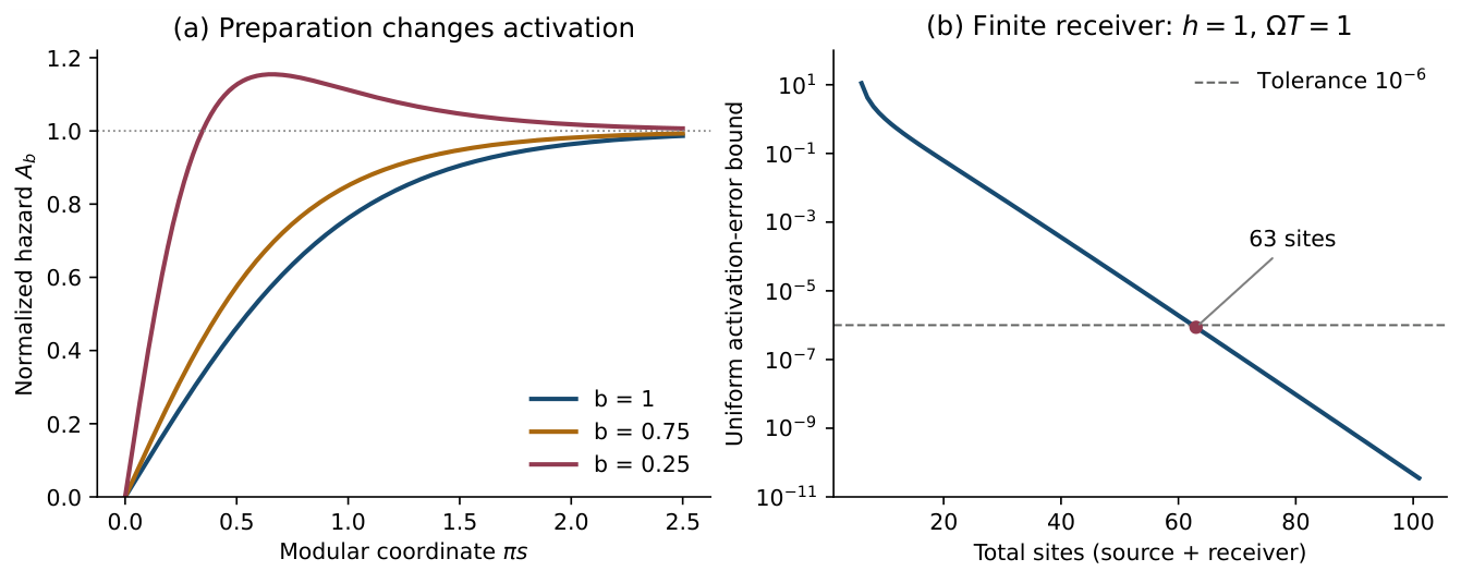
Table 3.
One fixed HP source at (seed 2026082100). The observer rows use the same late detector.
| Accessible radiation | Normalized information | (bits) |
|---|---|---|
| Global transmitted reference | ||
| Observer, no early radiation | ||
| Observer, all early radiation |
Disclaimer/Publisher’s Note: The statements, opinions and data contained in all publications are solely those of the individual author(s) and contributor(s) and not of MDPI and/or the editor(s). MDPI and/or the editor(s) disclaim responsibility for any injury to people or property resulting from any ideas, methods, instructions or products referred to in the content. |
© 2026 by the authors. Licensee MDPI, Basel, Switzerland. This article is an open access article distributed under the terms and conditions of the Creative Commons Attribution (CC BY) license (http://creativecommons.org/licenses/by/4.0/).
Copyright: This open access article is published under a Creative Commons CC BY 4.0 license, which permit the free download, distribution, and reuse, provided that the author and preprint are cited in any reuse.