

Submitted:
19 July 2026
Posted:
21 July 2026
You are already at the latest version
Abstract
We derive a causal law of observer-indexed entropy retrieval: retrieved reference information grows toward the supply available to a finite observer. A recorded admission-and-readout instrument produces orthogonal operational sectors from arbitrary coherent radiation; exact diary fidelity and decoupling give the flagged family, while branch errors bound its approximate realization. An exact quantum transfer channel yields the remaining-gap law and its continuous Lindblad evolution. The channel has an explicit unitary collision realization: admitted reference information moves from radiation to memory, while the capture record remains diary-blind. Its memory marginal is the Choi state of an erasure channel, giving an intrinsic positive-coherent-information boundary at retrieved fraction r = 1/2. A strip-holomorphic modular speed limit bounds how rapidly the channel can activate, with the hyperbolic tangent selected uniquely at extremality. The integrated retrieval dose is invariant under a change of clock, making the Kerr lapse cancellation one geometric instance of a general result. At fixed supply and kinetic rate under an affine clock, the transfer and activation laws compose into a closed proper-time retrieval trajectory on the equality branch, identify that trajectory as the sharp fastest-retrieval envelope, and fix the earliest admissible retrieval horizon. In the continuum formulation, Araki relative entropy defines retrieval on restricted observable algebras, and a split Type-I factor provides the regulated density-operator representation. The experimental program follows the same causal sequence through retrospective analysis and staged intervention. Tier 0A determines whether archived analog-horizon data retain the shot-level, timing, protocol, and processing information needed to ask the retrieval question. Tier 0B then tests whether qualifying data contain observer-, protocol-, readout-, or analysis-operator-indexed correlation structure that standard pooling or filtering suppresses. A positive Tier 0B result identifies retrieval-relevant structure and motivates Tier 1; it does not by itself confirm the complete law. The prospective Tier 1 BEC program targets the held-out g²(t₁,t₂) surface, bandwidth scaling, and protocol dependence. Independent activation readout tests the modular bound and tanh rigidity. Reference-tagged supply and memory test cumulative dose, composite-hazard recovery, degraded-channel ordering, and two-memory allocation. The v2 verification artifact provides synthetic benchmarks and numerical consistency checks at bond dimensions D = 4 and D = 8 for the transfer law, inverse recovery, finite-resolution robustness, and matched adversarial alternatives. Standard RT/HRT geometry and a separate accessibility functional place the retrieval dynamics within holographic language. The retrieval law closes the observer-local path between global encoding and retained access. Information conservation, radiation encoding, causal collection, finite-observer retrieval, formal reconstruction, and comprehension are distinct physical operations. The black-hole information problem contains a proper-time access dynamics that global entropy accounting alone does not determine. Physical complexity enters through encoding, supply, clock, activation, transfer, retention, and observation. Those layers locate each source of retrieval failure instead of idealizing it away. The theory orders the encoding, supply, and retrieval clocks; distinguishes late supply from early supply through their overlap with future transfer dose; and gives an exact finite-lifetime retrieval criterion. Here rᵢ(τ) is the normalized reference information retained by observer i, eᵢ(τ) is the causally available supply, kᵢ(τ) is the composite access hazard, and τ_char is the characteristic activation scale.
Keywords:
black hole information paradox
; observer-indexed entropy retrieval
; quantum channels
; modular flow
; quantum information theory
; proper-time dynamics
; Schwarz–Pick theorem
; analog gravity
; Bose–Einstein condensates
; second-order correlation functions (g²)
1. Reader’s Guide (How to Read This Paper)
This paper introduces a new way to think about information: not simply as something stored or globally conserved, but as something accessed by an observer in time.
It began with a simple question: What if entropy is not about what exists, but about what becomes accessible to an observer?
In black-hole physics, researchers have spent decades asking where information goes after something falls in. Existing programs address global entropy, reconstruction, and even decoding, but they do not derive the causal proper-time transfer law by which a specified reference correlation enters and remains in a finite observer’s memory. The unresolved operational question is not only whether information persists, but how a finite observer comes to retain the specified correlation.
This work derives a retrieval law for how information becomes accessible to an observer in proper time: not all at once, not just at the end, but gradually, along the observer’s path through spacetime.
The law is derived through an exact quantum transfer channel and constrained by modular analytic methods. It yields testable analog-black-hole signatures. It is invertible at the level of the composite access hazard: can be inferred from measured retrieval when the accessible supply is independently specified.
If you are not a physicist, that is fine. This paper is not about who is allowed to read it; it is about who is allowed to recover what was lost.
The paper is organized as follows:
- Section 2 derives the observer-indexed retrieval law and presents an inverse map that reconstructs the composite access hazard from measured retrieval and independently specified accessible supply.
- Section 4.1 defines the operational extraction of from measured correlation structure.
- Section 5 presents a finite-bond-dimension tensor-network proxy used to test access-law consistency and finite-resolution robustness.
- Section 6 translates the theory into the second-order correlation fringe measurable in current BEC analogs and lays out the Tier 0A data-recoverability audit, Tier 0B retrospective retrieval-surface audit, and prospective Tier 1 experiment.
- Section 7.4 defines the retrieval–termination gap .
- Appendix A formalizes the reference-information ceiling, exact transfer law, terminal-dose conditions, and modular activation bound. Appendix E states the split-property regularization and Type III1 continuum limit while keeping the split distance distinct from detector resolution.
- Appendix G maps , , , , , and to gravitationally intuitive quantities for readers unfamiliar with modular dynamics, without changing the retrieval law.
Note on this version.
Earlier versions did not adequately distinguish the mathematical ground of the transfer law from the analytic ground of the activation bound. The corrected separation is explicit: a flagged CPTP transfer channel and its GKSL limit derive the remaining-gap law, whereas strip contractivity bounds channel activation and selects the hyperbolic tangent only on the equality branch. Derived quantities are now distinguished throughout from supplied state and protocol inputs, independently calibrated factors, and projected observables. The most consequential additions are the operational derivation and controlled approximation of the flagged family, its unitary collision realization and exact reference-information balance, the intrinsic positive-coherent-information boundary, and the staged Tier 0A, Tier 0B, and Tier 1 test sequence. Remaining microscopic completions are a concrete detector-restricted modular activation, a radiation-to-readout realization, and a covariant observer–field interaction with backreaction.
2. Introduction
The causal-access problem sits inside black-hole information recovery: when does encoded information reach and remain with a finite observer?
This work establishes a causal law for when information becomes accessible to a bounded observer. Entropy accounting, decoding, and global reconstruction remain separate; the law governs the proper-time dynamics of access.
2.1. Entropy without Access: The Operational Gap
The black-hole information paradox remains open at the level of finite-observer retrieval because none of the programs evaluated here derives a causal law for that retrieval in observer proper time. Replica-wormhole paths and island prescriptions [1,2,3], ensemble Page-curve models [4,5], and dualities
[32] constrain entropy or reconstruction, yet none specifies the Lorentzian proper-time channel that carries a particular diary correlation into retained observer memory. Stabilizing global entropy or establishing reconstructability without that transfer law leaves finite-observer recovery undetermined. This paper derives that process.
Independent laboratory experiments on non-gravitational quantum systems have demonstrated bounds on the rate at which coherence becomes accessible [35]. They establish access time as a measurable physical clock.
Within the disk-contracting analytic class used here, Schwarz–Pick contraction bounds the onset of the transfer channel. Extremal rigidity selects the hyperbolic tangent at the speed limit. The transfer law then converts that activation into a retrieved-information trajectory.
The operational chain is
The first relation records global encoding in the radiation algebra. The first arrow restricts that encoding to what can causally reach observer i. The second transfers available reference information into retained memory. These are three different physical events. One quantity tracks each, so global availability is never mistaken for local possession.
The paper follows one diary through this sequence. The reference Q identifies the information being tracked. The global curve records its encoding in radiation; records the portion available to observer protocol i; records whether the transfer channel is active at detector setting b; records the composite transfer rate; and records what the observer has retained.
The diary correlation then moves through one conserved flow. Causal collection determines the admitted budget; a unitary collision then moves that budget from radiation into memory while the capture record remains diary-blind. When the retained fraction crosses one half, the memory acquires positive coherent information, and the modular speed limit determines the earliest observer time at which that crossing can occur.
Local quantum-field algebras remain Type III in the continuum [16,28]. A split inclusion provides a regulated Type-I factor on which density-operator expressions may be used, while Araki relative entropy remains the primary definition. The split distance regulates the algebraic representation. Finite switching, spectral response, and detector resolution define the observer protocol.
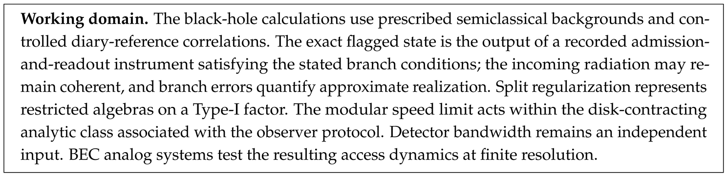
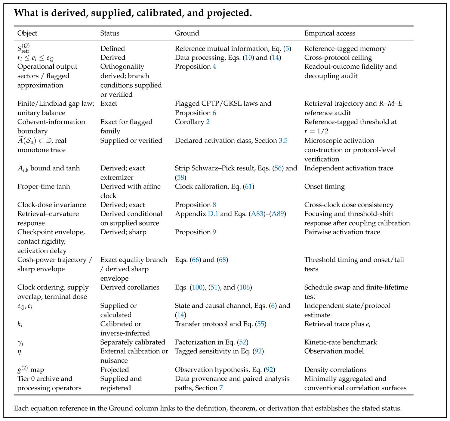
The exact transfer theorem and the modular activation theorem govern different steps. The first derives how the remaining information gap closes. The second derives the fastest admissible onset within the stated analytic class.
The table maps each object to its status and empirical access: what is defined or supplied, what is derived, and what enters through state, protocol, calibration, or observation.
2.2. Relation to Algebraic Entropy and Crossed-Product Constructions
Recent work in algebraic quantum field theory has clarified a foundational issue underlying gravitational entropy: how entropy may be meaningfully defined for systems whose local algebras are Type III and therefore admit no trace. In particular, crossed-product constructions developed by Chandrasekaran, Penington, and Witten, building on earlier modular and algebraic work by Longo and Takesaki, give rigorous constructions in which entropy is finite and well posed for quantum field theories with gravitational relevance [17,28,30,31].
These results resolve definability: what it means for entropy to exist as a mathematical quantity in relativistic quantum systems where density-matrix notions fail.
Crossed-product and related algebraic constructions establish the algebraic status of entropy and modular structure. This paper begins at the next physical step: the Lorentzian transfer of that entropy into a finite observer’s retained memory. The resulting transfer law imposes rate bounds and proper-time constraints and identifies observer-indexed access conditions.
2.3. Operational–Access Criterion
Entropy conservation, formal reconstruction, and finite-observer retrieval are distinct operations. The programs compared below present themselves as accounts of unitarity, information return, reconstruction, decoding, or resolution of the black-hole information paradox. Hayden–Preskill is especially important to the framing because it states the diary problem in the language of recovery and decoding [6].
The distinction begins with the observer. In global entropy and reconstruction arguments, the observer often enters through an access condition: the relevant radiation algebra is available, the decoding map exists, or the entanglement wedge is reconstructible. Those statements answer the questions for which they were built. They do not yet describe a finite physical system moving along a worldline, receiving only causally admitted modes, operating through a bounded detector and memory, and acting for finite proper time. ODER makes that observer part of the dynamics.
Global availability does not settle local possession. Once the observer is physical, access becomes a causal transfer process with a supply, activation, rate, threshold, and clock.
The operational-access problem has four physical requirements:
- 1.
- Proper-time delivery: requires an explicit dynamical map from an available carrier into a finite observer’s retained memory as that observer’s proper time unfolds. A Page time, decoding time, entropy transition, or statement of reconstructability does not by itself satisfy the criterion. A checkmark requires a proper-time transfer process ending in observer-local possession.
- 2.
- Lorentzian causal delivery: requires the access step to be located in a causal Lorentzian process with a declared worldline, causal support, or physical delivery channel. Euclidean saddles, entropy identities, or an abstract decoding map do not alone satisfy it. A checkmark requires an explicit Lorentzian causal structure governing the relevant recovery step.
- 3.
- Physics-grounded recovery structure: requires the program’s native information-return or reconstruction result to follow from a specified quantum-information or gravitational construction. Phenomenological curve matching or a qualitative recovery narrative does not satisfy it. A checkmark marks a derived recovery or reconstruction structure, including generalized- entropy saddle constructions; it does not imply that the program also supplies finite-observer delivery.
- 4.
- Empirical operationalization: requires a measurable protocol that maps the proposed access dynamics to observer-indexed laboratory quantities under controlled resolution, calibration, and held-out prediction. A computational proxy or a qualitative observational analogy does not alone satisfy it. A checkmark requires a specified experimental protocol capable of testing the access step itself at resolvable timescales.
The following table evaluates whether the major black-hole information programs include each operational-access requirement. It evaluates this stated problem, not the separate questions those programs were built to answer. A cross marks an operational step that the program does not provide; it does not mark failure at the program’s native objective.

Table 1.
Coverage of the operational-access criteria by major black-hole information proposals. A check marks an explicit component satisfying the criterion as defined above. A cross marks an unprovided operational step, not failure at the framework’s native objective.
Table 1.
Coverage of the operational-access criteria by major black-hole information proposals. A check marks an explicit component satisfying the criterion as defined above. A cross marks an unprovided operational step, not failure at the framework’s native objective.
| Framework | (a) | (b) | (c) | (d) |
| Replica wormholes | × | × | × | |
| Islands | × | × | × | |
| Hayden–Preskill | × | × | × | |
| Ensemble Page models | × | × | × | × |
| × | × | × | × |
Among the evaluated programs, replica wormholes, islands, and Hayden–Preskill satisfy criterion (c); none satisfies criteria (a), (b), or (d). None therefore derives a causal, observer-accessible retrieval channel in proper time. Entropy accounting determines the global information budget, and reconstruction determines the existence of a decoding map. Neither determines when a finite observer acquires and retains the encoded information. Resolving the operational-access problem requires the additional retrieval law derived here. This comparison therefore supplements, rather than displaces, the programs’ results at the encoding, unitarity, or reconstruction layers.
2.4. Retrieval, Reconstruction, and Comprehension: Non-Equivalence
Throughout this work we distinguish five logically distinct stages:
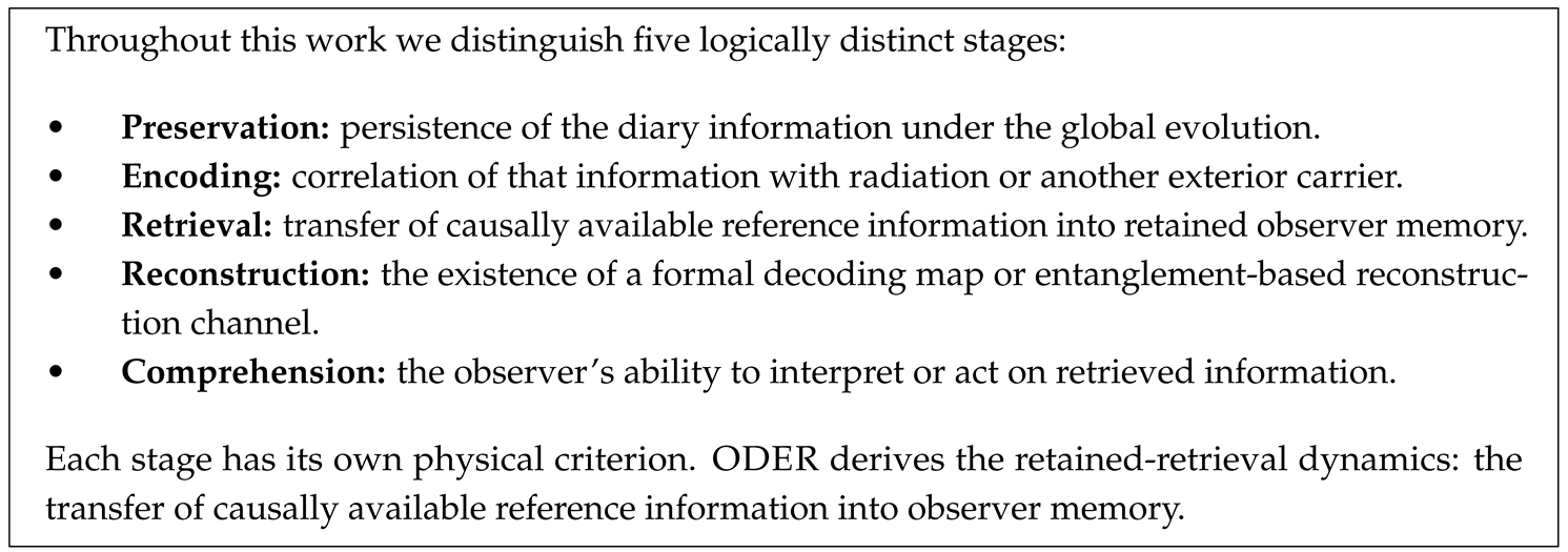
Throughout, we enforce the non-equivalence:
A reconstructable state can remain outside an observer’s memory; a retrieved state can remain uninterpreted. These are different physical events.
The argument proceeds in three layers: the remaining-gap transfer law, the strip-holomorphic limit on activation, and the experimental projection of their composition.
The claim operates at the level of access dynamics. It supplements entropy curves and reconstruction protocols with the observer-indexed transfer step needed to turn an available encoding into retained information.
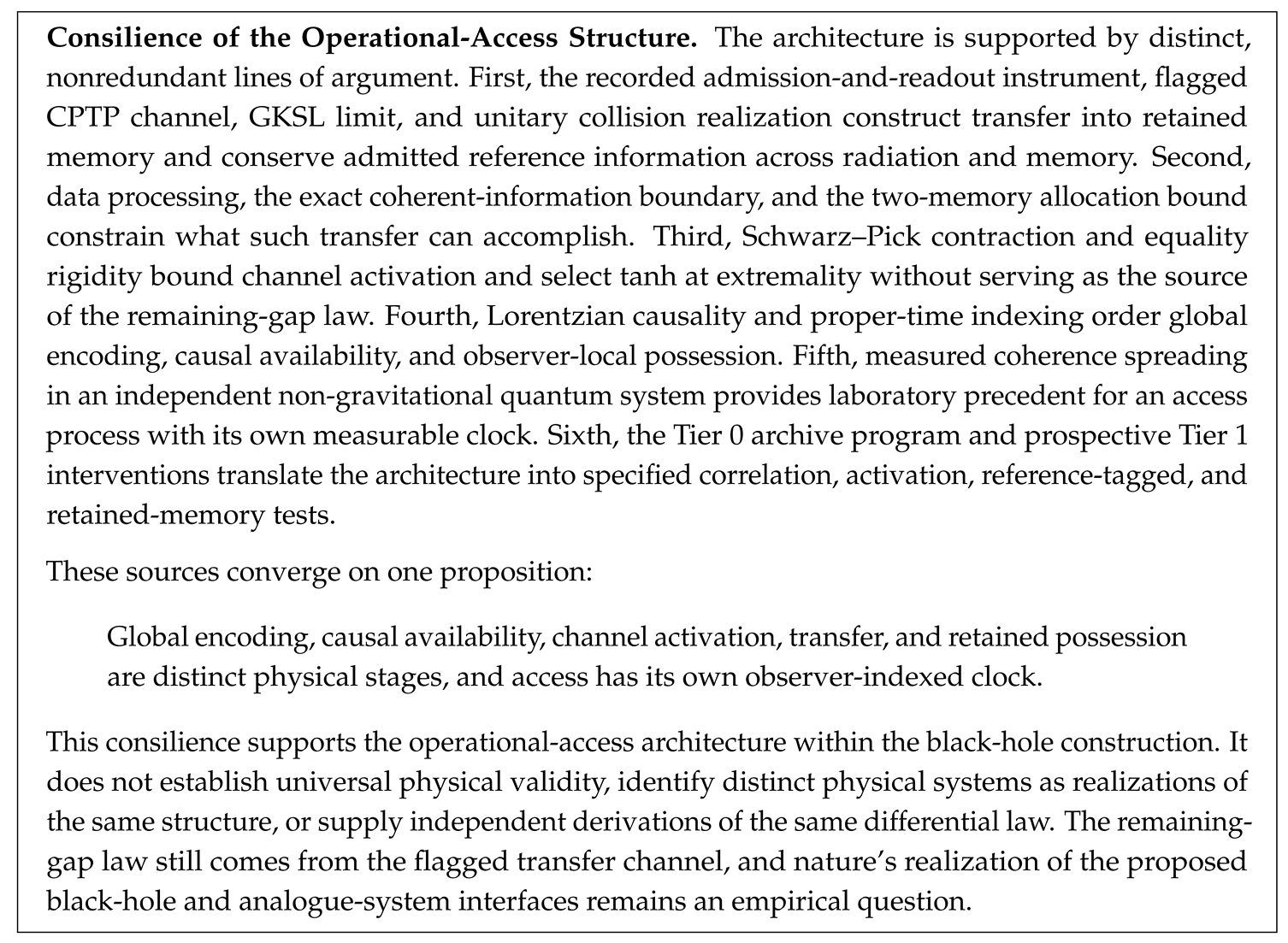
The consequence is that ODER changes the object of the problem. Preservation, encoding, retrieval, reconstruction, and comprehension are different physical events. Treating global existence or formal reconstructability as finite-observer possession is the category error that produces the operational-access form of the paradox. The law developed here closes that gap in proper time within its declared physical domain.
Black-hole information recovery is the forcing case in which the distinction between global encoding and finite-observer possession becomes unavoidable. The channel theorem states that distinction abstractly, while its physical validity here rests entirely on the black-hole state, causal supply, proper-time clock, transfer protocol, and observation map specified in this paper.
3. Observer-Dependent Entropy Retrieval
The order matters: identify the diary correlation, distinguish global encoding from causal supply, and then ask what enters retained memory. From those quantities follow the transfer law and the modular limit on how quickly transfer can begin.
3.1. Reference-Defined Retrieved Entropy
Throughout, logarithms are natural and we use units unless stated otherwise.
The reference fixes the information being followed. It remains outside the transfer process and records whether the diary correlation has reached the observer’s memory.
Let be a diary initially purified by a reference . For the exact channel construction below the initial state is maximally entangled,
For any identified d-dimensional data register X, write . More general diary states can be studied, but the linear formulas proved in Section 3.3 are special to the maximally entangled, orthogonally flagged model.
In algebraic quantum field theory, a local observable algebra need not admit a density matrix. For normal states and on the relevant von Neumann algebra, define
where is Araki relative entropy [29]. This is the primary modular-algebraic information quantity.
For split-regularized localization we assume a split inclusion
where is a Type-I factor and is a spatial split distance [27]. On that regulated factor, Eq. (2) has the density-operator representation
When the individual von Neumann entropies are finite, this reduces to . The relative-entropy definition remains primary when those separate entropies are infinite. The split property provides the regulated factorization. The observer protocol fixes the detector cutoff. These are independent controls: regulates localization, while the detector passband fixes the operational spectral window.
Definition 1
(Reference-retrieved entropy). For observer protocol i, let be the retained quantum memory through proper time τ. Define
For a perfect purification transferred to memory, and . Equation (5) measures diary correlation, with the controlled diary entropy as its ceiling. Memory entropy and black-hole entropy measure different objects.
In the general case, is the reference-correlation functional. Operational message recovery adds a decoder and a success criterion such as entanglement fidelity or coherent information. In the flagged erasure family, the success branch carries a perfect purification of Q and the orthogonal flag identifies the transfer outcome exactly; Corollary 2 derives its coherent information and the intrinsic boundary.
3.2. Global Encoding, Causal Supply, and the Access Ceiling
Radiation encoding and observer access occur at different stages. The variables in this subsection separate them before the retrieval dynamics begin.
Let denote cumulative outgoing radiation through retarded time u. Define the global diary-encoding curve
The selected quantum state and radiation model determine this curve. A Page curve tracks a global entropy partition; tracks the radiation encoding of a specified diary. For a diary injected into an old black hole, these transitions occur on different clocks. The diary-specific recovery question is the operational lineage of Hayden–Preskill protocols [6]; the present construction separates their global encoding stage from observer-local possession.
An observer protocol is the tuple
containing its worldline, coupling, switching, detector setting (including aperture and passband), retained memory, operational lifetime, and readout operations. Let be the radiation modes inside that protocol’s causal support and collection band. A restriction channel and a memory channel define
where is the latest retarded emission time able to influence the observer by .
To retain the residual collectable radiation as well as the memory, define a joint causal output channel
whose memory marginal satisfies . The register contains modes admitted by the same causal support, aperture, and passband but not yet transferred to retained memory.
Proposition 1
(Causal data-processing ceiling). If the memory begins uncorrelated with Q and is generated by the channels in Eq. (8), then
Proof.
Apply monotonicity of relative entropy to and then to . □
Proposition 2
(No observer-independent positive lower bound). Fix the global state of at a given retarded time. Over the unrestricted channel envelope, global radiation data impose no positive lower bound on .
Proof.
An identity channel attains . A replacement channel , independent of , gives . □
The observer class therefore contains a collection channel or has zero collection capacity. Within a specified physical class, causal support and detector response can make the achievable ceiling strictly smaller than the global radiation bound.
Proposition 3
(Retrieval-deficit decomposition). Suppose the diary is initially purified by the full system and let be generated from the cumulative radiation by the observer’s causal channel. Then
Every bracket is nonnegative. They are, respectively, the global encoding deficit, the causal-collection deficit, and the retained-transfer deficit.
Proof.
The identity telescopes. The first term is nonnegative because . The second follows from the observer-channel data-processing inequality, and the third follows by tracing out . □
When all quantities are normalized by , Eq. (11) becomes
Within this factorization and joint-channel convention, the identity partitions the terminal deficit into global emission, causal collection, and local transfer. The selected channels fix the partition; their respective dynamics supply the three terms.
The coherent-information criterion adds a threshold structure to this additive accounting. If the causal-collection ceiling never exceeds , then prevents positive coherent information no matter how completely the transfer deficit is closed. The collection deficit can therefore remove the positive-coherent-information horizon rather than merely delay it. When , the transfer dynamics determine whether and when the observer crosses that boundary.
Corollary 1
(Three-stage complete-recovery criterion). At a fixed observer time, complete retained recovery occurs if and only if all three deficits in Eq. (12) vanish:
Thus complete global diary encoding is necessary but does not by itself establish causal collection or retained possession.
For the exact model below, the relevant supply is
where is causally accessible residual radiation and is retained memory. This total accessible budget obeys . Its radiation component is the remainder
3.3. Operationally Flagged Transfer and the Supply-Limited Law
Once diary information is available to an observer, the remaining question is local and dynamical: how does it cross from accessible radiation into retained memory? The following channel answers that question exactly for an orthogonally flagged transfer process. Its assumptions identify the physical family governed by the resulting law.
The orthogonal flags belong to the observer’s recorded admission and readout outcomes. They need not be present as a block decomposition of the incoming Hawking radiation. The next proposition makes that operational origin explicit.
Let both R and M have a d-dimensional data sector and an orthogonal erasure flag . For , define
The three operational retrieval sectors are orthogonal: the diary is retained in memory with weight r, remains in accessible radiation with weight , or is unavailable with weight .
Proposition 4
(Operational emergence of the flagged family). Let S denote arbitrary microscopic radiation degrees of freedom and let be any joint state with , including a coherent or scrambled radiation state. Let be a three-outcome quantum instrument from S to , with its outcomes recorded in mutually orthogonal output sectors corresponding to retained, admitted-but-unretained, and unavailable diary information. Write
If, for some , the subnormalized branch states are the three corresponding summands in Eq. (16), then . No block-diagonality assumption on is required.
More generally, let denote the three ideal branch states in Eq. (16). If
then
Proof.
Recording the instrument outcome in orthogonal sectors removes cross terms between the three readout outcomes. Under the exact branch conditions, their sum is Eq. (16). The approximate statement follows from linearity and the triangle inequality for the trace norm. □
The proposition separates two questions. Orthogonality is supplied by a recorded observer outcome; diary-faithful recovery on the retained branch and diary decoupling on the unavailable branch determine how closely a concrete decoder realizes the ideal family. The exact model below is the zero-error instrument output. The proposition does not assert that every radiation state admits such a zero-error decoder. A microscopic black-hole realization must construct or verify the branch conditions for its chosen radiation state and decoder.
Theorem 1
(Exact reference information). For the state in Eq. (16),
Consequently, and is the normalized reference information remaining in accessible radiation.
Proof.
Each reduced state is a flagged erasure state. Orthogonality makes its entropy the Shannon entropy of the branch weights plus the average entropy within each branch. The binary flagged channel with transmission probability has
and hence . Taking , e, and for M, , and R, respectively, proves Eq. (19). A direct three-block calculation gives the same result for . □
The memory marginal contains a second operational statement that is not visible from its mutual information alone. Define the d-dimensional erasure channel with transmission probability r by
Corollary 2
Its coherent information [10] is
Thus positive coherent information begins at the intrinsic boundary . Under independent memoryless uses of the erasure channel, its quantum capacity is [7]
The capacity is understood in the standard asymptotic channel sense [8]. Since , an observer for whom cannot cross the positive-coherent-information boundary, irrespective of transfer rate or lifetime.
Proof.
Tracing R in Eq. (16) combines the residual-radiation and unavailable branches into the erasure branch of Eq. (21). The flagged-state entropy calculation gives and , proving Eq. (22). Equation (23) is the memoryless quantum-capacity formula for the erasure channel. The supply-floor statement follows from . □
Here r is the retained fraction produced by the observer’s retrieval dynamics, not a free channel parameter. The erasure boundary becomes a proper-time retrieval horizon.
Let P project onto the sector in which R contains diary data and M contains the erasure flag. Let V be the partial isometry
For , define
Because , is completely positive and trace preserving.
Proposition 5
(Canonical exact bounded readout). Let be a two-outcome exact readout instrument on the admitted radiation–memory system. Suppose successful capture acts with a common probability on a readable subspace P, so that , and suppose the no-capture operator is the positive nondisturbing branch. Trace preservation then forces
for a partial isometry V with . If the captured output is stored entirely in a d-dimensional memory data sector while the residual radiation is reset to one erasure state, then . Thus an exact memory smaller than the admitted field can read a code subspace, not uniformly and faithfully transfer the entire field.
Proof.
Completeness gives . Positivity of the no-capture branch selects its positive square root, . The polar decomposition of gives . The rank bound follows because a partial isometry preserves the dimension of its initial space and its captured range lies in the memory data sector. □
Equation (25) is therefore the canonical positive nondisturbing realization of exact, uniformly heralded capture on the readable sector. General approximate, nonuniform, or disturbing instruments need not take this form.
Theorem 2
(Exact retained-memory transfer). The channel in Eq. (25) preserves already retained diary information and satisfies
Thus the exact finite-step update is
Proof.
transfers only the residual-radiation branch to the orthogonal memory-data branch. leaves the memory and unavailable branches invariant and retains weight in the residual-radiation branch. Collecting the three orthogonal blocks gives Eq. (27). □
Equation (27) is the reduced description of a unitary capture event. The enlarged dynamics identify where the admitted reference information remains and exactly what the capture record knows.
Proposition 6
(Unitary realization, diary-blind record, and reference balance). Let have basis and define
Then , so is the restriction of a unitary on to the initialized subspace , and
For ,
and the capture record is diary-blind:
Thus the environment records whether capture occurred while the admitted diary-reference information remains entirely in the radiation–memory sector.
Proof.
Orthogonality of the record states and Kraus completeness give . The finite-dimensional isometry extends to a unitary, and tracing its record gives Eq. (30). The marginal is , so Eq. (19) gives Eq. (31). Directly tracing gives
which proves . Local isometry preserves , while the marginal has the same mutual information. The chain rule then proves the conditional identity. □
The unitary can be chosen constructively. With , set
On the residual branch,
while the initialized retained and unavailable sectors are fixed. Tracing E gives with . For fresh record qubits and , the repeated-interaction limit [13] gives
so the finite channel and its GKSL evolution are the same unitary capture process at discrete and continuous resolution.
For a constant supply e and a sequence of independent transfer attempts , repeated application gives the exact discrete survival law
Thus the additive discrete dose is . The continuous dose is its weak-step limit. Exponential survival is therefore a consequence of channel composition.
The finite channel also has an exact continuous quantum-dynamical lift. With the same , so that , let
Proposition 7
(Continuous retained-memory channel). For fixed accessible supply e, the flagged family is invariant under Eq. (38), and its retained fraction satisfies
The exact propagator from to is the finite transfer channel with
Proof.
On the residual-radiation block, the anticommutator removes weight at rate and the jump term deposits the same weight in the retained-memory block. Hence , which proves Eq. (39). The generators at different times are scalar multiples of the same superoperator, so their propagator depends only on the cumulative dose. Equation (40) then follows from the survival factor . □
The finite channel and the Lindblad evolution are two resolutions of the same transfer process. One gives the exact update per capture opportunity; the other gives its proper-time flow. The remaining-gap law is therefore a quantum channel result at both finite and infinitesimal scale. Growth of the supply is the separate source process specified below.
If , the continuous-time limit is
Equivalently,
For unit step supply, Eq. (42) reduces to a saturation law with ceiling .
The remaining-gap form is the transport equation of the flagged reference sector. The partial-isometry capture moves the diary purification from accessible radiation into retained memory; repeated capture opportunities compose multiplicatively, and their GKSL limit gives Eq. (41). At detector level, Section 4.2 realizes the same hazard as , separating the rate of admissible capture opportunities from their reference-sensitive retention probability. The black-hole state sets the causal information budget, while the gap dependence follows from the transfer channel itself.
The theorem governs a maximally entangled diary with orthogonal operational outcome flags, a recorded readout state block diagonal in those sectors, Markovian transfer from residual radiation, lossless retained memory, and externally supplied nonnegative . Proposition 4 shows that this block structure is an output of the declared instrument and does not require the incoming Hawking radiation itself to be block diagonal. At every transfer step the diary correlation occupies R or M; the channel transfers it without cloning it.
For time-dependent , the larger source evolution is additionally assumed to induce compatible reduced updates
between transfer steps. This source update moves newly admitted diary correlation into the accessible outcome sector while preserving both the recorded readout structure and the retained memory. It is the black-hole supply input, acting on the larger source system between local transfer steps.
3.4. Time-dependent supply
Let , , and let be measurable with , so that . Define
Theorem 3
(Integral solution and ceiling preservation). The unique absolutely continuous solution of Eq. (41) with is
If , , , and , then
Proof.
Equation (45) follows from the integrating factor. For ,
Nonnegativity of follows directly from Eq. (45). □
Corollary 3
(Reference-information continuity). Along a supplied differentiable flagged path, define the normalized memory, residual-radiation, and total admitted inventories by
With transfer current and incoming supply current , they obey
At fixed supply,
The source changes the admitted reference budget; the observer channel moves that budget from residual radiation into retained memory.
Proof.
This is the conservation law behind the retrieval dynamics: causal collection changes the admitted budget, while observer-local transfer changes its allocation between radiation and memory.
Corollary 4
(Supply–access overlap). Under the hypotheses of the preceding theorem, for any terminal time T,
Proof.
In Eq. (45), set , so that , and integrate the source term by parts. □
Equation (51) weights each increment of admitted diary information at time s by the transfer dose remaining after its arrival. Earlier increments receive at least as much future transfer as later increments, and information admitted at T has no time to enter memory. Access opportunities do not act retroactively: final supply and total dose alone do not determine retrieval unless their ordering along the observer’s proper-time channel is also specified.
Decreasing supply belongs to a larger channel family: an explicit joint residual-loss/source channel must preserve . Memory loss is represented by a lossy-memory term or a non-Markovian channel. The present theorem governs monotone supply and lossless retained memory.
3.5. Retrieval as a Modular Speed Limit
The transfer channel determines how an available information gap closes. Modular analyticity answers the next question: how quickly can that channel turn on? The two results meet through the factorization of the composite hazard.
The strip-to-disk speed limit and its equality and rigidity consequences are developed independently in Ref. [36]; the present section states the interface required by the black-hole instantiation.
Factor the composite hazard as
where is the calibrated activation and the kinetic traversal rate. Before imposing an activation profile, the rate-density character of the composite hazard gives a general clock result.
Proposition 8
(Clock-reparameterization invariance of retrieval dose). Let be an increasing absolutely continuous change of clock with almost everywhere. If satisfy the retrieval law on the τ clock, define
Then the same remaining-gap law holds on the λ clock and
If activation is treated as a scalar trace under the change of clock, the same statement holds with : the kinetic factor transforms as a rate density and the integrated composite dose is invariant.
Proof.
The chain rule gives . Equation (54) is the corresponding change of variables in the dose integral. □
Clock conversion therefore cannot create retrieval dose by itself. Any physical enhancement must change the state, admitted supply, activation, base transition process, or duration of the admissible protocol. The Kerr lapse cancellation in Section 8.2 and Appendix F is a geometric instance of this general result.
The retrieval trajectory determines the composite hazard,
where the denominator is positive. Independent supply estimates turn Eq. (55) into an inverse diagnostic. Held-out traces then test the recovered hazard.
Introduce a dimensionless analytic coordinate s and a centered profile . Assume that its real trace is real-valued and nondecreasing and that . Schwarz–Pick contraction for the strip gives
For the stated strip normalization, . Integration gives the sharp post-onset envelope
If a nonconstant map saturates the infinitesimal Schwarz–Pick metric at an interior point, rigidity makes it a conformal isometry. Centering, reality, and orientation then select the unique extremizer
The physical post-onset activation is
with onset alignment and orientation
so that the post-onset branch satisfies . The independently calibrated map converts the analytic coordinate into observer proper time. Equations (56)–(59) govern activation; the exact transfer channel governs and . The split property provides the regulated algebraic representation, and the analytic class imposes the modular speed limit.
When the calibrated clock is affine, with , the extremal activation takes the proper-time form
Proposition 9
(Checkpoint envelope, contact rigidity, and activation delay). Let lie in the calibrated post-onset interval, and write and . Every activation in the declared analytic class obeys
Equivalently,
Define the accumulated activation delay
It is additive across consecutive proper-time intervals. Equality in Eq. (62) for one distinct pair forces the complete activation onto the extremal tanh branch. Under the affine calibration in Eq. (61), the proper-time separation between two activation levels satisfies
with equality only on the extremal branch.
Proof.
Divide Eq. (56) by and integrate from to . Applying the addition formula for tanh gives Eq. (63). Equation (64) is the nonnegative integrated speed deficit, so additivity follows from additivity of the integral. Equality for one distinct pair makes the continuous pointwise deficit vanish on the intervening interval. Equality at any interior point invokes Schwarz–Pick rigidity and fixes the full tanh profile. The affine threshold bound follows from . □
Corollary 5
(Extremal proper-time retrieval). Let the supply and kinetic rate be constant after , and let the activation saturate Eq. (56) under the affine calibration in Eq. (61). If , then
Equivalently, the cumulative retrieval dose obeys
Proof.
Insert Eq. (61) into and integrate from to . □
Proposition 10
(Sharp retrieval envelope and earliest horizon). Assume the constant supply e, constant kinetic rate , and affine clock used in the preceding corollary, but allow any activation in the declared analytic class. Then, for ,
Equality holds on the extremal tanh branch. For , the operational retrieval horizon therefore obeys
The bound is sharp and is attained by the extremal branch. If and , no finite retrieval horizon exists within the continuous finite-rate model.
Proof.
The activation envelope gives
Corollary 6
(Positive-coherent-information horizon). Under the hypotheses of Proposition 10, assume and define
Then
The bound is attained by the extremal branch. If , no positive-coherent-information horizon exists. For unit supply and , the crossing requires the exact dose
and on the extremal branch, with ,
Proof.
The two appearances of encode different operations that meet on the extremal branch. Equation (72) is the dose required to halve the unit-supply retrieval gap. The modular latency is the total activation deficit relative to a channel fully open at onset:
When , capacity is crossed in the kinetic tail and
The first term is the half-gap time of a channel fully open at onset and the second is its modular latency. When , the crossing lies in the activation-limited quadratic regime:
Thus the intrinsic quantum threshold resolves the same activation-to-kinetic crossover already visible in the onset and tail of the retrieval trajectory.
Corollary 7
(Activation-limited onset and kinetic tail). Let . On the extremal branch, as ,
so and . At late time,
Relative to a channel fully activated at , the fastest analytic onset therefore has the late-time equivalent delay
The hyperbolic tangent is therefore the extremal activation profile, while the cosh-power curve is the fastest retrieved-information trajectory admitted by the analytic class at fixed supply and kinetic rate. The onset is activation-limited and quadratic; the late tail is kinetic and exponential. The onset curvature and late log-gap slope separately determine and instead of fitting only their product; the closed formulas are given in Eq. (A64). The derivation closes the proper-time chain from modular onset to an earliest retrieval horizon without identifying activation with accumulated retrieval.
3.6. Laboratory Precedent for a Measurable Access Clock
Ultracold-atom experiments on Bose–Einstein condensate formation provide an independent physical precedent for access-limited quantum dynamics [35]. Once the scaling regime is reached, the measured coherence length satisfies
with a universal late-time coarsening rate despite interaction-dependent early-time transients and offsets. The result constrains the rate at which long-range coherence becomes accessible; it is distinct from a transport or signaling velocity.
This laboratory result establishes that access to organized quantum structure can carry its own measurable clock. It is independent empirical precedent for the broader operational distinction used here: a physical structure may exist before it becomes accessible at the measured scale. It does not confirm the black-hole remaining-gap law, the proposed radiation-to-memory channel, or the tanh activation profile. In this paper those elements retain separate grounds: the flagged-channel construction derives the transfer law, and the strip theorem bounds activation within its declared analytic class.
Failure of coherence-speed bounds in the appropriate homogeneous quantum systems would constrain the broader proposition that access to retrievable structure exhibits universal rate limitation. It would leave the exact remaining-gap transfer theorem intact and sharpen the question of which physical systems realize the disk-contracting activation class.
4. Observer-Dependent Entropy in Curved Spacetime
The same radiation state can produce different retrieval histories because observers do not share a worldline, causal support, detector, or memory. This section turns those physical differences into observer protocols and follows their consequences in proper time.
The trajectory and detector protocol determine which modes can contribute to . With an independent estimate of that supply, the retrieval trace determines the composite hazard through Eq. (55). Separating into requires one of those factors to be calibrated independently. This division of labor follows the status map in the Introduction.
4.1. Classification of Observers
The three observer classes enter through distinct kinetic factors : stationary exterior access, freely falling post-crossing access, and acceleration-conditioned access. The calibrated activation then forms the composite hazard . Figure 1 shows the kinetic profiles used in the verification benchmark.
Table 2.
Representative parameter values for each observer class ( in geometric units). The retrieval horizon is defined by in the unit-supply benchmark. The access marker is a profile parameter, not the global Page time. Retrieval-horizon values match the v2 verification artifact. All reported proper-time origins are onset-aligned by the declared common benchmark comparison clock; the table does not order raw proper times on unrelated worldlines.
Table 2.
Representative parameter values for each observer class ( in geometric units). The retrieval horizon is defined by in the unit-supply benchmark. The access marker is a profile parameter, not the global Page time. Retrieval-horizon values match the v2 verification artifact. All reported proper-time origins are onset-aligned by the declared common benchmark comparison clock; the table does not order raw proper times on unrelated worldlines.
| Observer | |||||
| Stationary | 10 | 0 | 5 | 8 | 30.5 |
| Freely falling | 0 | 2 | 4 | 12.9 | |
| Accelerating | – | 0.2 | 3 | 5 | 20.5 |
Retrieval ordering follows from channel structure. When one observer channel is physically degraded from another, data processing fixes the order exactly.
Proposition 11
(Ordering under observer-channel degradation). Suppose that, at proper time τ, observer j’s memory channel is a CPTP post-processing of observer i’s channel,
Then
Proof.
Apply data processing to and normalize by . □
Equation (82) supports controlled comparisons of nested apertures, passbands, or post-processing chains when the degradation map is established. The benchmark classes below explore broader protocol differences for which no universal ordering follows.
Stationary observer.
A detector at fixed Schwarzschild radius samples a redshifted field state with local Tolman temperature . If the benchmark kinetic process has an approximately constant factor per Schwarzschild time, conversion to static-observer proper time gives
This clock-conversion benchmark isolates the redshift contribution. Switching, coupling, aperture, passband, and the diary correlation in the admitted modes complete the kinetic factor; multiplication by the calibrated activation gives the physical hazard .
Freely falling observer.
A geodesic world line crosses the horizon at . Along a geodesic world line, the causal mode support and detector response change through horizon crossing. The benchmark used here assigns a rapid post-crossing increase in , written schematically as
This step-like post-crossing profile is a calibrated access-window benchmark, not a universal locally detectable effect of crossing a smooth horizon. An infalling retained record is local possession along that worldline; it becomes exterior recovery only if the declared readout lies in an exterior-accessible causal future. The protocols determine the free-fall and stationary ordering; the degradation proposition determines it whenever their channels are nested.
Accelerating observer.
A uniformly accelerating detector has an acceleration-dependent response. For an Unruh–DeWitt coupling with switching [18], the relevant finite-time response is
from which the protocol-specific kinetic factor is calibrated. Acceleration enters through this response rather than through a free-standing power law.
Experimental mapping.
Stationary and accelerating channels can be engineered in waterfall BEC analogs through controlled flow and detector configurations, while freely falling access is approximated by a rapid access-window or channel-change protocol after the horizon-crossing analog. The synthetic study adopts signal-to-noise ratio and a target temporal resolution near as design conditions. They are benchmark requirements rather than consequences of the retrieval law.
4.2. Detector Response and Reference-Information Transfer
The response functional in Eq. (85) gives the detector excitation probability for a specified coupling and switching. Retrieval is the reference-sensitive component of that response. Correlation with Q separates diary-bearing excitations from thermal and vacuum backgrounds.
As a one-wavepacket benchmark, let be a selected outgoing packet inside the protocol support and let be a retained memory mode. On the branch in which carries the diary data, a number-preserving capture interaction implements
with orthogonal records for capture and noncapture. Tracing the record reproduces the transfer channel in Eq. (25). On the captured branch the purification is moved into memory; it is not copied. Equations (34)–(36) give the corresponding repeated-interaction unitary, while Eq. (32) shows that the capture record learns the event without learning the diary.
Suppose independently resolved capture opportunities form a Poisson process of intensity and a reference-correlated opportunity is retained with conditional probability . Over an interval with approximately constant parameters, the probability of no successful capture is
Combining this survival factor with Eq. (37) gives the continuous hazard
Here is calibrated from detector response, while contains mode overlap, transfer efficiency, and reference sensitivity. Their product separates the information hazard from the thermal count rate and realizes the exact remaining-gap law at detector level.
4.3. Observer-Dependent Entropy
Observer-dependent retrieved entropy is the reference-correlation quantity defined in Eq. (5). Its instantaneous ceiling is , the diary information within the observer’s causal collection and memory channel. The remaining transfer gap is therefore , rather than a difference between two unspecified entropy scales.
4.4. Retrieval Law (Instantiation)
For the flagged-transfer family derived in Section 3, the observer instantiation is
In the unit-supply benchmark, . If the equality activation is selected and is independently specified, Eq. (89) recovers the original proper-time saturation model. The three profiles in Figure 1 are calibrated kinetic factors ; they combine with the independently declared activation to form the composite hazard .
4.5. Inherited Speed-Limit Constraint
The observer-class trajectories introduce no new speed-limit principle. They use the activation constraint in Section 3.5. Within its strip-holomorphic class, the hyperbolic tangent is the equality profile for activation. It is not imposed on itself. Observer protocols change the causal supply , the kinetic factor , the calibrated activation clock, and therefore the composite hazard . Distinct proper-time signatures follow when those calibrated inputs differ.
5. Quantum Information Correlations and Testable Predictions
Current correlation imaging measures the projected retrieval surface. A fixed measurement map carries the proper-time trajectory into observable correlation structure, allowing held-out tests of the causal sequence against matched alternatives.
Observer dependence is defined by the worldline, causal support, switching, coupling, aperture, passband, retained memory, and operational lifetime of the observer protocol.
The projection follows one dependency chain:
Activation enters the primary observation model through the transfer law and the resulting retrieval trajectory.
The retrieval law in Eq. (89) constrains the latent reference-information trajectory. A measurement model is still required to relate that trajectory to radiation observables. We consider two diagnostics: the order- Rényi entropy of the selected subsystem and the second-order correlation function . Neither observable equals without an explicit state and detector map.
The forward model is tested under held-out protocol conditions. Baseline correlation parameters are calibrated before retrieval fits; supply is estimated independently; the latent trajectory determines the composite hazard; and the calibrated dynamics must predict new correlation surfaces.
Simulation traces with confidence bands for each class are shown in Figure 2. Bands are generated from 200 resampled traces per observer class, with the benchmark activation held fixed, on a common proper-time grid with the synthetic noise model.
5.1. Rényi Entropy and Second-Order Correlation Functions
Observer-indexed differences in access translate into distinct protocol classes in analog systems, implemented through controlled variations in flow configuration and detection geometry.
For any subsystem A, the Rényi entropy is
with . Equation (91) arises by analytically continuing the integer-order moments (the replica trick); for a field-theoretic derivation see Casini, Huerta, and Myers [20]. Larger heightens sensitivity to eigenvalue gaps; therefore probes the observer-dependent delay . Here functions as a theoretical purity diagnostic, while the directly modeled analog observable below is , accessible through density–density correlation measurements in BEC analog systems [19].
To project the retrieval dynamics into a measurable correlation surface, let
Times are measured relative to the onset-aligned analysis window, with after baseline alignment. Let be the decorrelation time measured in the no-retrieval baseline. Define the connected excess correlation . A modeled suppressive envelope is
where and are fixed by baseline data. The sensitivity is fixed by an external tagged-retrieval calibration or profiled as a nuisance parameter; a zero-retrieval baseline identifies no factor multiplying . Equation (92) is monotone in each for positive baseline amplitude, so certified degraded-channel ordering survives in the projected suppression envelope. The equation is the measurement hypothesis linking the latent reference trajectory to density correlations.
On the constant-supply, constant- extremal benchmark, Eq. (66) gives
The tanh activation reaches the correlation surface through the derived retrieval trajectory.
The synthetic waterfall-BEC benchmark uses an effective correlation time near and a target sampling interval of . These are design values for the power study. Experimental feasibility must be established from the cadence, integration window, and noise properties of the selected platform.
The non-retrieval null sets and leaves the symmetric exponential baseline. Matched thermal, diffusive, and generic-saturation alternatives are then compared against the full protocol-conditioned surface.
Parameters are extracted with nonlinear least squares from ensemble realizations consistent with the admissible observer constraints.
Within this forward model, captures decay-modulated suppression associated with observer-indexed access, while tracks the spectrum of the independently measured subsystem state.
Controlled comparisons among observer protocols test the projected final link in Eq. (90). Independent activation measurements and reference-tagged memory close the preceding links.
Table 3.
Core observer-class retrieval diagnostics in the v2 verification artifact. The retrieval horizon is defined by in the unit-supply benchmark. Threshold times use the onset-aligned common benchmark comparison clock.
Table 3.
Core observer-class retrieval diagnostics in the v2 verification artifact. The retrieval horizon is defined by in the unit-supply benchmark. Threshold times use the onset-aligned common benchmark comparison clock.
| Observer | Final | Bounded | Monotone | Inverse pass | Median error | ||
| Free falling | 2.0 | 12.9 | 1.000000 | Yes | Yes | Yes | 0.003178 |
| Accelerating | 3.0 | 20.5 | 0.999863 | Yes | Yes | Yes | 0.000924 |
| Stationary | 5.0 | 30.5 | 0.981079 | Yes | Yes | Yes | 0.000364 |
Because the retrieval law is first order and gap-dependent, a retrieval trace with independently supplied determines . Dividing by the calibrated activation recovers on the positive-activation window. Figure 3 shows that second step in the verification benchmark.
5.2. Activation, Dose, and Held-Out Prediction
The prospective Tier 1 experiment tests relations among independently identified quantities. Baseline data fix and ; the selected state and collection protocol supply ; a separate detector calibration fixes or the activation observable. Retrieval data are then divided into calibration and held-out conditions.
For a baseline-normalized, delay-window-reduced envelope, the extremal constant-supply benchmark is
where is Eq. (66). With and calibrated, and with fixed by an external tagged condition, the onset scale is the remaining trajectory parameter. When is not fixed in advance, it is profiled as a nuisance parameter and the held-out surface remains untouched until prediction.
A nonlinear least-squares estimator minimizes
When is fixed by external tagged calibration, this is a one-parameter minimization over .
The modular speed limit is tested on an independently calibrated activation trace through
For an affine clock on the equality branch, . Because differentiation becomes ill-conditioned near saturation, the registered test window is restricted to , with smoothing, derivative estimation, and uncertainty propagation fixed before evaluation.
The checkpoint form in Eq. (63) gives a derivative-free activation test. Every registered pair must satisfy that envelope using the independently calibrated clock difference . Exact contact for one distinct pair forces the complete tanh equality branch within the analytic class. The accumulated quantity in Eq. (64) measures subextremal activation delay and must compose additively across adjacent acquisition windows. Under affine calibration, measured activation thresholds additionally test Eq. (65). These pairwise diagnostics remain available when the nominal onset time is uncertain.
The transfer law yields a second diagnostic. Define
Under the extremal constant-, constant- benchmark, Eq. (67) predicts that is linear in . Sequential capture windows must also compose additively in .
The non-retrieval null sets . Thermal, diffusive, generic-saturation, and non-gap alternatives are matched in parameter count. Calibration data determine the model parameters; a separate protocol or bandwidth condition tests the predicted , dose, and full surface.
The registered analysis requires (i) on the evaluation window, (ii) nonnegative and sufficiently smooth , (iii) independent estimates of the quantities placed in the denominator of Eqs. (55), (95), and (96), (iv) and , and (v) .
The v2 verification artifact records the calibration split, bootstrap seeds, derivative window, error propagation, residuals, and held-out predictions. Varying detector bandwidth tests the onset scaling while keeping the analog background and analysis protocol fixed.
6. Holographic Connection and MERA-Inspired Finite-Resolution Proxy
Wedges, redshifted surfaces, and finite-resolution reconstruction depth give the observer-indexed retrieval law a geometric representation tied to the experimental access variables.
Placed beside standard RT/HRT geometry, the retrieval law acquires a geometric interpretation in terms of observer-dependent access to a fixed entanglement wedge. A lapse- and protocol-weighted accessibility functional records the accessible portion of that fixed geometry. The corresponding 48-qubit MERA-inspired proxy tests the same bounded-access constraint at finite resolution. Qubit count and bond dimension control the resolution of the representation.
The resulting representation links the retrieval law, its spectral constraints, and its observable signatures within a single geometric interpretive structure.
6.1. Observer-Indexed Mapping to Ryu–Takayanagi Geometry
The RT/HRT entropy is retained in its standard form [33,34]. For a boundary region A with extremal surface ,
with the classical RT/HRT limit obtained when the bulk correction is neglected. The observer protocol selects the part of the associated wedge that can be causally sampled and retained. Redshift enters through the observer clock.
- : the standard RT/HRT extremal surface;
- : a protocol-dependent accessibility weight encoding causal reach, aperture, passband, and collection time.
Define the dimensionless geometric accessibility score
The associated entropy-valued weighted area contribution is . Thus measures the fraction of a fixed geometric encoding admitted by the observer protocol, while remains the reference-information quantity. Redshift enters the calibration of through the observer clock and detector response. This construction is compatible with recent crossed-product and edge-mode algebra treatments [17,23] of gravitational entropy and modular structure.
Under refinement of the split regulator, the algebraic mutual information and geometric encoding are compared within a fixed state and code subspace. The detector passband remains a separate control. These quantities provide a boundary–bulk representation of access. The RT surface fixes the geometric encoding datum; the observer protocol fixes the weighted accessibility score. An explicit boundary-to-observer channel determines and .
The following mapping translates retrieval-rate classes into experimentally accessible signatures associated with the same observer-indexed access structure.
The tanh equality activation is available to every protocol satisfying the same analytic and clock assumptions; it is not an acceleration-specific profile. Each kinetic-rate profile maps to an observer patch in the boosted bulk representation and to a correlation signature in Table 4. Detector resolution fixes the effective resolution of that patch. Declaring the modular regulator, geometric regulator, detector passband, and clock places all three descriptions on a common comparison surface.
7. Experimental Signatures and Measurement Conditions
The analogue-system boundary is authoritative for every test in this section. BEC analogues do not reproduce an evaporating gravitational black hole. They isolate the field-propagation, correlation, and finite-observer access layer of the proposed construction. They do not establish global black-hole unitarity, gravitational backreaction, or microscopic Hawking encoding. Success or failure therefore applies first to the controlled analogue realization; transfer to the gravitational setting requires the additional physical completions stated in Section 9.
Within that boundary, the BEC program reaches the black-hole argument’s latent sequence along retrospective and prospective paths. The current-platform measurement primitive resolves the projected retrieval surface, bandwidth response, and protocol dependence. An independent activation readout adds the modular speed-limit test. Reference-tagged sources and retained memories add direct measurements of supply, retrieval, dose, and inverse hazard.
The central observable is the two-point correlation function reconstructed from density–density correlations or equivalent detector outputs. Equation (92) connects that observable to the latent retrieval trajectory.
The experimentally relevant control parameters are: flow configuration, including horizon formation profile and gradients; detection configuration, including temporal windowing, sampling cadence, and channel extraction; effective detector bandwidth, defined by temporal resolution or spectral cutoff; and baseline normalization across repeated condensate realizations.
Distinct protocol classes are implemented through controlled variations in these parameters. Stationary, accelerating, and freely falling access label protocols that instantiate controlled analogues of the corresponding access conditions.
The registered discriminant combines the exact remaining-gap law, the declared disk-contracting activation class, and the forward model. Direct tests of the sharp envelope, supply–access overlap, and terminal-dose criterion additionally require independently fixed supply, kinetic rate, and retained-memory readout.
7.1. From Retrospective Structure to Prospective Intervention
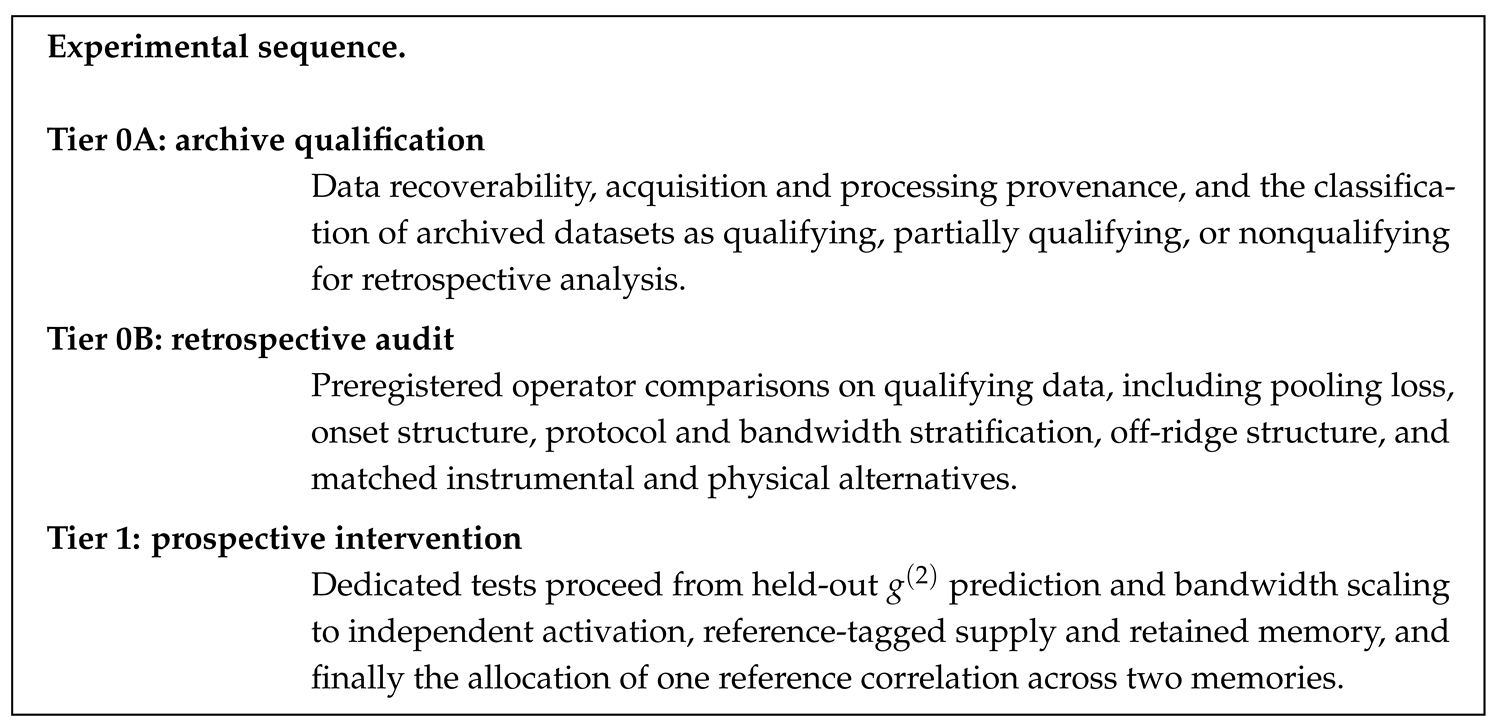
Tier 0A qualifies an archive by determining whether the measurements and processing provenance needed for an access analysis remain available. Tier 0B then nominates viable correlation structures, processing operators, controls, and feasibility requirements from qualifying data. Those outputs become a locked Tier 1 design. Tier 1 manipulates the nominated access variables on new runs, independently measures the latent quantities required by each claim, and evaluates predictions on conditions held out from calibration.
Tier 0B nominates the signature; Tier 1 freezes and tests it.
7.2. Tier 0 Retrospective Retrieval-Surface Audit
Tier 0A: data-recoverability and provenance audit.
Tier 0A is a pre-analysis assessment of whether an existing analog-gravity BEC dataset preserves enough information to support an observer-, protocol-, readout-, or analysis-operator-indexed retrieval analysis. It inventories shot-level or minimally aggregated measurements, acquisition and horizon-formation timing, protocol and detector settings, spatial and temporal resolution, calibration and run-quality records, intermediate density and correlation products, and every documented smoothing, filtering, alignment, exclusion, and pooling operation. A qualifying dataset supports the complete Tier 0B audit; a partially qualifying dataset supports only named retrieval questions; and a nonqualifying dataset has lost or never recorded the necessary structure. Tier 0A does not test the retrieval law. It establishes whether the question remains empirically askable in the archive.
Tier 0B: retrospective retrieval-surface audit.
Tier 0B is a preregistered reanalysis of a Tier 0A-qualified dataset. It compares the structure preserved under minimally aggregated analysis with the structure produced by conventional pooling, filtering, temporal alignment, bandwidth restriction, and stationary-horizon analysis. The audit tests aggregation loss, time-resolved onset, protocol and bandwidth dependence, off-ridge or delayed correlation structure, and matched alternatives including horizon thickness, scattering, atom loss, thermal background, imaging response, and calibration drift. Deliberate operator perturbations ask whether candidate structure is preserved, weakened, shifted, or erased in the registered direction.
A positive Tier 0B result requires organized structure that is recoverable from the archived measurements, varies systematically with declared access or analysis conditions, survives matched physical and instrumental alternatives, and responds predictably to specified processing operators. Such a result identifies retrieval-relevant structure and fixes the interventions needed for Tier 1. It does not by itself confirm the complete ODER law. Only analog-horizon datasets containing the required density or correlation measurements can directly test the analogue-horizon observation-level retrieval-surface hypothesis at Tier 0B; other BEC relaxation or coherence datasets remain proxy tests of inverse-retrieval machinery.
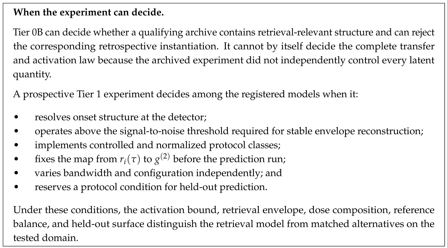
Transition to Tier 1. The analysis now turns from retrospective nomination to prospective intervention. The subsections that follow specify the locked Tier 1 predictions, measurement conditions, and discriminants to be tested on new runs.
7.3. Constrained Saturation and Suppression Envelope
Under Eq. (92), the connected correlation envelope inherits the bounded activation, remaining-gap transfer, and asymptotic saturation of the latent trajectory. The current-platform projected test is the complete held-out correlation surface. An independently measured activation trace tests Eq. (95); reference-tagged and test the dose relation in Eq. (96).
Onset is smooth and monotone. The extremal branch has constant under affine calibration. The retrieved fraction follows Eq. (66), and sequential windows add in cumulative dose. It is the sharp fastest trajectory in the analytic class, with quadratic onset and a late exponential tail. The onset curvature and late log-gap slope separate the activation width from the kinetic rate through Eq. (A64). The lossless Markovian benchmark approaches its supply without overshoot or revival. Against a calibrated fully open control, the equality branch also predicts the asymptotic tail shift .
Measurement Condition.
Resolving this structure requires sufficient bandwidth to distinguish onset curvature from detector smoothing. The registered interior window keeps the derivative diagnostic away from saturation, where finite differences become unstable.
Discriminant.
Thermal, diffusive, and generic-saturation models are held-out alternatives. The test asks whether they reproduce the same activation bound, dose composition, earliest-threshold bound, onset/tail scale separation, bandwidth response, and out-of-sample correlation surface under matched parameter counts.
7.4. Protocol-Dependent Separation
The calibrated forward model assigns distinct envelopes to protocols with different supplies, clocks, and transfer hazards. A stronger ordering result is available when one protocol is a certified degradation of another.
Protocol classes vary flow and detection configuration under matched initial conditions, normalized amplitude, and fixed bandwidth. Certified nested apertures, passbands, or post-processing chains additionally test Eq. (82). Because Eq. (92) is monotone in , greater retained retrieval produces greater projected suppression for positive baseline amplitude.
Measurement Condition.
The test requires matched condensate states, explicit normalization, a fixed observation map, and a demonstrated CPTP or classical post-processing relation for any pair advertised as degraded. Two nominally different bandwidths do not establish degradation by themselves.
Discriminant.
The held-out discriminant is the ordered full surface under a certified degradation chain, not amplitude separation alone.
7.5. Observer-Resolution Dependence of Onset Time
When the activation clock is passband limited, the characteristic onset time scales inversely with effective detector bandwidth.
Increasing effective bandwidth by a factor b then shifts by approximately . The comparison tracks onset position, the registered window, and the held-out envelope after the measured instrument response is applied.
The gravitational and laboratory clocks require separate calibrations. With and , the geometric timescale bridge is
An analogue experiment must independently establish the map between its horizon scale and laboratory time; the geometric conversion does not provide that calibration.
Measurement Condition.
Bandwidth is varied across multiple regimes while condensate preparation, flow configuration, protocol definition, and analysis window remain fixed.
Discriminant.
The measured detector response enters every null and alternative. The finite-band prediction is the joint recovery of inverse onset scaling, activation structure, and held-out protocol separation after that response is included.
7.6. Protocol Asymmetry and Reference-Information Allocation
Controlled mismatch between normalized detector channels or access windows changes the projected suppression relative to the matched baseline. This is a current-platform projected comparison. A prospective Tier 1 reference-tagged two-memory experiment tests the stronger quantum allocation result.
For disjoint retained memories and in the same joint state with one reference Q, weak monotonicity implies
The inequality governs allocation of a common reference correlation. It is distinct from acceleration-dependent interference and from comparisons across separately prepared runs. Within the flagged erasure family, Corollary 2 gives exactly when . Consequently two disjoint memories in one joint state cannot both cross the positive-coherent-information boundary for the same diary reference. The high-threshold exclusion is thus the dynamical channel-level expression of the no-cloning allocation constraint [14], rather than a consequence of the chosen reporting threshold.
Measurement Condition.
The registered current-platform comparison uses matched baselines, controlled asymmetric configurations, and repeated runs. The next-generation test prepares a common reference-tagged excitation and records two disjoint memory outputs on the same run.
Discriminant.
Protocol asymmetry must predict the held-out correlation geometry after drift, decoherence, and detector response are fitted on baseline data. The prospective reference-tagged experiment separately tests Eq. (99). At a common threshold , it also tests the sharper implication that one memory at forces the other to satisfy in the same joint state. At the intrinsic boundary, that experiment asks whether either memory acquires positive coherent information while the joint allocation law prevents both from doing so.
Table 5.
Verification, proposed retrospective, adversarial, and robustness diagnostics. Status labels distinguish completed numerical checks from the Tier 0 archival program and the registered prospective tests.
Table 5.
Verification, proposed retrospective, adversarial, and robustness diagnostics. Status labels distinguish completed numerical checks from the Tier 0 archival program and the registered prospective tests.
| Diagnostic | Status | Interpretation |
| Tier 0A archive qualification | Proposed retrospective audit | Determines whether shot-level data and processing provenance support the registered Tier 0B questions |
| Tier 0B operator audit | Proposed retrospective reanalysis | Tests whether pooling, filtering, alignment, or bandwidth operations predictably preserve, shift, weaken, or erase retrieval-relevant structure |
| Calibrated observer ordering | Pass | on the onset-aligned common benchmark clock |
| Bootstrap confidence bands | 200 traces/class | Matches the v2 verification artifact |
| Finite-resolution proxy | Ordering and boundedness survive resolution variation | |
| Activation-ratio test | Registered interior window | Tests the speed limit separately from extremal saturation |
| Log-cosh dose test | Equality-branch benchmark | Tests composition of tanh activation with gap transfer |
| Sharp retrieval envelope | Registered supply and kinetic rate | Tests the earliest admissible threshold and finite-lifetime no-go |
| Onset/tail/latency consistency | Equality branch plus fully open control | Tests quadratic onset, late kinetic decay, and |
| Supply–access schedule swap | Tier 1 reference-tagged | Tests the future-dose weighting of an admitted diary pulse |
| Reference-balance and record null | Tier 1 reference-tagged | Tests Eqs. (31), (50), and (32) against loss or leakage |
| Coherent-information crossing | Tier 1 reference-tagged | Tests the intrinsic boundary and its supply floor |
| Held-out surface | Separate protocol condition | Tests prediction rather than same-trace reconstruction |
| Proper-time jitter | Ordering survives | Horizon ordering is stable to time perturbation |
| Non-gap dynamics null | Inverse recovery unstable | Gap-form structure matters |
| Observer-label permutation | Chance-baseline calibration | Calibrates the expected strict-order chance baseline |
7.7. Operational Falsifiability
Tier 0A produces a feasibility classification rather than a test result. For a qualifying archive, Tier 0B can establish or reject retrieval-relevant structure for that dataset under the registered operator comparisons. A null Tier 0B result does not reject the transfer law unless the archived protocol also independently fixes the supply, activation, kinetic rate, and observation map required by the corresponding claim. Tier 1 supplies those prospective controls.
- Violation of Eq. (95) rejects the stated analytic activation class on the calibrated interior window.
- Satisfaction of the bound without equality supports bounded activation while rejecting the extremal tanh branch for that protocol.
- Failure of the log-cosh or sequential-dose relations rejects the constant-supply, lossless Markovian transfer benchmark.
- Failure of the quadratic onset or late kinetic-tail relations rejects the extremal constant-supply branch even when a generic saturation fit passes.
- A reference-tagged schedule swap tests Eq. (51): moving the same admitted supply pulse earlier or later relative to a fixed transfer window must change terminal retrieval according to the remaining future dose.
- At fixed admitted supply, a reference-tagged audit must satisfy while the capture record satisfies . Failure rejects the lossless flagged transfer family even when the retained-memory trace is well fit by a sigmoid.
- Failure of a preregistered held-out surface rejects the calibrated observation-level instantiation.
- Violation of certified degradation ordering rejects the stated post-processing relation. Violation of the same-state two-memory bound rejects the common-reference, disjoint-memory implementation or its estimator.
7.8. Numerical Verification and Synthetic Benchmarks
The v2 verification artifact evaluates the constrained retrieval dynamics through the finite-resolution MERA-inspired proxy lineage described in Appendix C. The proxy encodes the access law and tests its numerical consequences under controlled resolution.
Within this realization: finite detector resolution is represented through restricted access depth; retrieval proceeds within a causal-cone–restricted proxy structure; and observer-indexed protocol variation is implemented through boundary and channel transformations.
The resulting numerical trajectories reproduce the same observable structure described above: a constrained saturation or suppression envelope, observer-class separation, inverse-rate recovery under known activation, finite-resolution robustness, and adversarial-null discrimination.
The realization demonstrates that the combined pattern arises under finite, computationally tractable access conditions. Its correspondence with the BEC protocol is structural: both implement bounded access under finite resolution.
The same retrieval structure can be projected into a correlation-level observable through the modeled envelope. Figure 4 illustrates the corresponding bounded-access signature in a controlled numerical setting.
8. Operational Consequences and Falsifiable Predictions
The preceding derivations follow diary information from radiation encoding into retained memory. That sequence changes the information paradox, creates distinct retrieval boundaries, and determines which experiments can distinguish its physical instantiations.
The exact channel gives the remaining-gap law, modular analyticity bounds activation, and the analog protocols test their combined consequences. The result is an observer-indexed retrieval layer on prescribed semiclassical backgrounds. It composes with global entropy and reconstruction results. It asks when an available encoding enters a finite observer’s retained memory.
Physical complexity determines where the retrieval chain is constrained, delayed, degraded, or terminated. Each effect enters through a specified physical layer and changes the observer’s retained record accordingly.
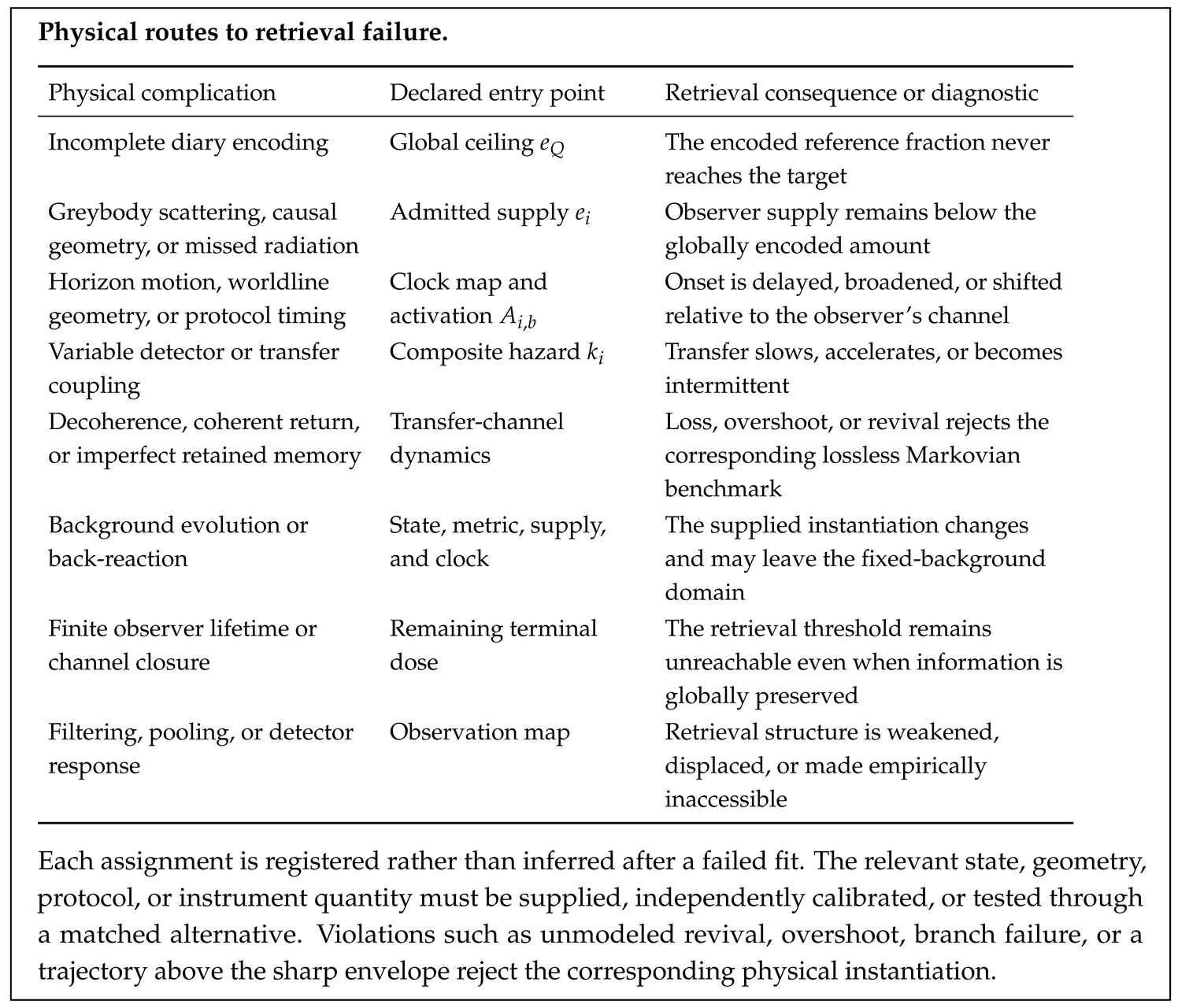
8.1. Operational Advance on the Information Paradox and Empirical Constraints
Existing approaches determine entropy and reconstruction structure. ODER derives the proper-time transfer law that carries an available encoding into finite-observer possession.
For the exact channel family, Eq. (89) drives retained reference information toward the causally available supply. The selected black-hole state and radiation model supply the diary-specific curve ; the Page curve tracks a separate global entropy partition. Tanh rigidity fixes the extremal channel onset, and Eq. (68) makes the resulting cosh-power curve the fastest admissible proper-time retrieval trajectory at fixed supply and kinetic rate.
For a common threshold , define the diary-encoding and admitted-supply times on observer i’s clock by
with the infimum of the empty set understood as .
Proposition 12
(Encoding–supply–retrieval chronology). For the declared observer channel,
Proof.
Equation (10) gives . The corresponding threshold sets are nested, so their first-hitting times have the stated order. □
The recovery clocks are therefore ordered. Diary information must be encoded before it can be admitted to an observer channel, and admitted before it can be retained. Global entropy and reconstruction transitions belong to the encoding and reconstructability layer; neither is, by itself, an observer’s recovery time. Conversely, high retained retrieval certifies sufficient global encoding, while low retained retrieval does not diagnose global information loss.
Island and replica constructions can determine generalized-entropy and reconstruction transitions [1,2,22]. A state-and-radiation model may use that structure to determine ; the explicit causal collection channel still determines . The present law then determines how the admitted reference information enters retained memory. These levels compose while preserving their distinct transition times and entropy variables [15].
8.2. Retrieval Horizon ≠ Entanglement Wedge ≠ Event Horizon
The retrieval architecture distinguishes three operational boundaries:
- Retrieval horizon. for a threshold , with used in the synthetic benchmarks.
- Entanglement wedge: the bulk region associated with the standard RT/HRT surface in Eq. (97).
- Event horizon: the classical null surface.
These boundaries describe different physical events for finite observers. No coincidence among them is assumed. Any coincidence is a model-dependent relation that must be established within the chosen geometry, state, and observer protocol.
Within the flagged channel, is a distinguished retrieval threshold rather than another geometric boundary. It marks the crossing of into positive coherent information. The conventional records high-fidelity operational attainment; under independent memoryless uses, the capacity threshold records the earlier point at which the erasure channel can first support nonzero asymptotic quantum transmission.
The integral solution makes this separation dynamical. For locally integrable and admissible bounded , the retained trajectory is absolutely continuous. A sharp change in reconstruction, admitted supply, detector response, or horizon-crossing kinematics may change , but it cannot by itself deposit a finite diary fraction into memory at one instant:
On the extremal analytic branch, Eq. (77) strengthens this statement to a quadratic post-onset opening.
In Kerr spacetime, the stationary retrieval channel is defined relative to an admissible local generator , restricted to regions where
Within such timelike wedges, the stationary clock-conversion benchmark is
where contains protocol-specific switching, coupling, passband, and state response. The benchmark applies inside the timelike domain. Tanh activation follows when activation belongs to the disk-contracting analytic class and the calibrated clock is affine. Outside the stationary region, the appropriate description is a different trajectory or a nonstationary modular channel.
Writing gives . For the lapse-only clock conversion , Proposition 8 gives
The cancellation is the Kerr realization of the general clock-change identity: the apparent proper-time rate enhancement cancels the lapse in the integration measure. Redshift alone does not force divergent dose or complete retrieval near the null boundary; genuine enhancement must enter through the state, admitted supply, base transition rate, activation, or available duration.
8.3. Multi-Observer Retrieval as a Differential Test
Observer-dependent retrieval produces protocol-conditioned differences in the admitted supply, transfer hazard, and observed correlation surface. The single-observer law supports a differential-protocol test. Two disjoint memories in one joint state with the same reference also obey the allocation bound in Eq. (99).
For a common threshold , the allocation theorem gives the exact high-threshold exclusion
At the paper’s threshold, one disjoint memory at or above bounds the other at or below . This statement concerns one joint state, one diary reference, and disjoint physical memories. Separate protocol runs and multiple formal reconstruction maps do not constitute simultaneous independent records.
Certified channel degradation also orders threshold times. If at matched values of a declared comparison clock , then
Raw proper-time values on unrelated worldlines are not ordered without such a clock map.
When the fully calibrated forward model predicts separation above measurement uncertainty, two protocols must produce resolvably different reference-access curves and connected envelopes. Collapse to the same curve then falsifies that observer-indexed instantiation. The conditional prediction allows compensating changes in and and remains independent of Page-curve saturation.
8.4. : Retrieval–Evaporation Boundary
Diagnostic quantity. distinguishes threshold attainment from terminal retrieval failure. Define
with the relevant evaporation or termination time expressed in the same proper-time convention as the retrieval threshold. The retrieval horizon is defined operationally by the access threshold, not by the inflection point of the entropy-access curve. The inflection point is a separate curvature diagnostic of the retrieval trajectory, fixed on the extremal branch by Eq. (A63). Positive means the threshold is crossed before evaporation or termination; negative values mean that the threshold is not crossed within the available lifetime. The latter can result from insufficient supply, causal collection, or transfer dose and must be diagnosed with Eq. (11).
Proposition 13
(Finite-lifetime retrieval criterion). Suppose the admitted supply is constant at e on , with , and define . Then
For the analytic class with constant , affine clock, and , if
then no admissible activation reaches the threshold by T.
Proof.
The sign of is therefore a dose-budget statement. Exact attainment of from a nonzero gap requires divergent dose; finite-time retrieval horizons are necessarily operational thresholds.
Table 6.
Synthetic retrieval thresholds from the verification benchmark and the additional quantity required to evaluate . Thresholds are reported in M-scaled geometric units. The v2 verification artifact does not supply a protocol-specific terminal event on the same observer clock, so no sign is assigned.
Table 6.
Synthetic retrieval thresholds from the verification benchmark and the additional quantity required to evaluate . Thresholds are reported in M-scaled geometric units. The v2 verification artifact does not supply a protocol-specific terminal event on the same observer clock, so no sign is assigned.
| Observer | Terminal event on observer clock | status | |
| Stationary | Not specified | Not evaluated | |
| Freely falling | Not specified | Not evaluated | |
| Accelerating | Not specified | Not evaluated |
A negative in a numerical model or analog proxy is a terminal-readout failure for the protocol when the independently specified supply and hazard predict threshold crossing. A nonnegative value records threshold attainment; the activation, dose, and held-out tests decide the dynamics that produced it.
9. Domain of Validity and Completion Paths
The fixed-split result is complete within its declared channel, activation, background, and observation assumptions. Work beyond that domain has three different statuses. Defined next tests operationalize quantities already specified by the theory. Specified physical completions name the additional interaction, channel, or source required to extend a theorem’s physical domain. Longer-range extensions identify regimes whose full formalism has not yet been constructed. The boundaries below keep those statuses distinct.
9.1. Channel and Activation Boundary
The exact remaining-gap law applies to the flagged, Markovian transfer family with retained memory and an explicit unitary collision realization. The activation theorem applies separately to a real monotone trace in the declared disk-contracting strip-holomorphic class. Neither result asserts that generic microscopic Hawking radiation already arrives in exact operational sectors or that every detector realizes the extremal branch.
The immediate specified physical completion is a concrete detector-restricted modular observable whose activation trace can be shown to belong to the analytic class and whose clock can be independently calibrated. A second completion constructs the microscopic radiation-to-readout instrument and evaluates the branch fidelity and decoupling errors in Eq. (17). Imperfect readout branches, loss from retained memory, coherent competition, and non-Markovian return require enlarged channels and corresponding evolution equations. These completions test physical realization; they do not change the fixed-split channel theorem.
9.2. Fixed-Background Boundary
The retrieval dynamics use a prescribed background metric and quantum state. The access hazard and supply are evaluated on that background. The specified covariant completion begins with the observer–field interaction in Eq. (A72), derives and renormalizes its stress tensor, verifies covariant exchange, and solves the semiclassical Einstein equation together with the retrieval dynamics. Appendix D.1 states that source interface and its perturbative control parameter; Appendix D.2 gives the associated focusing response and first-order retrieval-horizon shift. Backreaction is established only after that microscopic source is supplied.
Intersecting horizons and overlapping causal diamonds are specified next geometric tests of how admitted supply and observer mismatch behave beyond a single prescribed channel. Superposed geometries are a longer-range extension requiring a state-dependent or relational access map rather than the fixed background modular generator. Stationary Kerr remains the controlled generator deformation in Appendix F; genuinely nonstationary and multi-horizon settings require additional relative-Tomita, edge-mode, and domain analysis [17].
9.3. Experimental and Observation Boundary
Equation (92) is a projected observation map, not a derivation from a specified analogue field and detector. Its physical completion must begin with the prepared reference, field dynamics, detector coupling, and retained-memory readout and derive the measured surface from those elements. Baseline normalization, instrument response, and the latent-to-observed map must be fixed before the prediction condition is opened.
The defined test sequence is canonical in Section 7: Tier 0A qualifies an archive, Tier 0B nominates structures and operators, and Tier 1 freezes and tests them on new runs. Tier 1 progresses from held-out correlation and bandwidth tests to independent activation, reference-tagged supply and memory, and the same-state two-memory allocation protocol. Cross-platform replication in photonic, superconducting-circuit, or other analogue systems requires comparable correlation measurements, declared observer protocols, and independent calibration rather than visual similarity of envelopes.
Observer-resolution scaling is a defined next test. For a calibrated detector family with , the prediction is . Equivalently,
over the registered scaling range. Onset curves should collapse against while the analogue background and protocol remain fixed. The split collar is varied independently: detector bandwidth is not an algebraic regulator. In the idealized high-bandwidth limit the activation delay can vanish, but the finite kinetic floor remains.
9.4. Simulation and Resolution Boundary
The v2 verification artifact reports synthetic benchmarks and numerical consistency checks at . Those outputs establish boundedness, benchmark ordering, inverse recovery under supplied inputs, finite-resolution robustness, and discrimination from the implemented adversarial alternatives. They do not establish a continuum limit or laboratory realization.
Defined next tests extend scaling beyond , propagate detector and model uncertainty into explicit error budgets and ROC-style sensitivity estimates, add adversarial access schedules and non-Markovian or lossy protocols, and test inverse- stability as resolution and noise vary. Inverse recovery of remains conditional on independently fixed activation. Regulator stability requires the split collar and detector protocol to be refined independently as specified in Appendix E.
9.5. Full-Recovery Boundary
The result proved here is retained reference transfer, not complete diary recovery. The boundary is the zero crossing; positive coherent information and, under independent memoryless uses, nonzero asymptotic quantum capacity begin for . It is not perfect decoding, high-fidelity diary reconstruction, or complete possession of the message. The reporting horizon is likewise an operational threshold rather than a universal recovery criterion.
Full recovery requires a specified decoder, an entanglement- or message- fidelity target, and a retained-memory model that includes loss during storage and readout. Memory loss can lower possession after transfer and therefore requires a channel beyond the lossless benchmark. Global unitarity, reconstruction, and microscopic decoding remain adjacent layers: they may supply or act on the retrieved state, but they are not identified with the transfer law.
Replica wormholes, islands, and topology-changing saddles can supply global encoding or reconstruction structure for without determining , , decoder fidelity, or retained-memory loss. Composing those layers is a specified completion path; equating their transitions with either or complete diary recovery is not.
10. Conclusion
This paper completes the observer-local encoding–supply–transfer–possession chain within its stated domain. A reference system identifies the diary correlation; global radiation encoding bounds the causally admitted supply; and retained memory defines possession. A recorded admission-and-readout instrument produces the operational sectors required by the exact flagged family, while explicit branch errors quantify its approximate realization.
The flagged CPTP channel and its GKSL limit derive the remaining-gap law. Their unitary collision realization transfers admitted reference information from radiation into memory while leaving the capture record diary-blind. Strip contractivity supplies a separate result: it bounds activation and selects the tanh profile only at equality. Under fixed supply, kinetic rate, and an affine clock, the two results compose into the sharp cosh-power retrieval envelope without conflating activation with transfer.
The completed structure orders the recovery clocks as , makes retrieval depend on the overlap of causal supply with remaining transfer dose, and distinguishes shortfalls in encoding, collection, and possession. The erasure-channel marginal places the intrinsic positive-coherent-information boundary at ; complete diary recovery still requires decoder fidelity and retained- memory integrity beyond that boundary.
Page curves, islands, replica wormholes, entanglement wedges, and decoding protocols determine neighboring questions of unitarity, encoding, or reconstructability. They can supply inputs to the observer channel, but they do not determine the Lorentzian proper-time transfer into a finite observer’s memory. The result established here is the missing dynamical relation between causal availability and retained possession on a prescribed background.
The retrieval–curvature construction in Appendices Appendix D.1 and Appendix D.2 specifies the interface for completing this fixed-background result with a renormalized microscopic observer–field source.
Retained reference information evolves toward the causally available supply under an exact remaining-gap law, while modular analyticity fixes the fastest admissible activation. Global encoding establishes possibility; constrained access establishes possession.
Global existence and finite-observer possession are different physical events. Conflating them creates the operational form of the paradox; the retrieval channel derived here gives the law that separates and connects them.
Information is not operationally present when it exists, but when it becomes accessible under constraint.
Author Contributions
E.C. conceived the study; developed the theory, methods, and software; performed the formal analysis and numerical verification; prepared the figures; and wrote and revised the manuscript.
Funding
This research received no external funding.
Data Availability Statement
The canonical v2 verification artifact for the current verification suite is notebooks/ODERBHverificationartifactv2.ipynb, archived with the project repository at https://github.com/evlocoo/ODER-modular-entropy and the Zenodo release record at https://zenodo.org/records/20721727. It runs in publication mode in a standard CPU/Jupyter environment and regenerates the report, manifest, figures, and diagnostic tables used for the retrieval-law verification suite.
- notebooks/ODERBHverificationartifactv2.ipynb: reproduces the core retrieval-law checks, inverse- recovery using the generating supply and known benchmark activation, finite-resolution robustness at , and adversarial-null diagnostics.
- outputs/verificationreport.md and outputs/validationmanifest.json: record the preset, thresholds, nulls executed, pass flags, and claim-to-artifact map.
- outputs/figures/ and outputs/tables/: contain the generated PNG figures and CSV diagnostic tables used to audit the verification suite.
Supporting finite-resolution materials document the archived legacy v1.1 MERA-inspired proxy lineage described inAppendix C. They generate bounded observer-access and finite-resolution proxy outputs.
- archive/v1.1/ODERBlackHoleFrameworkCompleteSimulation(V2).ipynb: documents the archived legacy proxy lineage, including the 48-qubit parameterization, observer-class retrieval profiles, and finite-resolution comparisons.
- archive/v1.1/ODERRetrievalInversionAndValidation.ipynb: documents retrieval-rate inversion, numerical consistency checks, and correlation-envelope diagnostics from the earlier proxy lineage.
No astrophysical or experimental BEC data are used in the present verification suite. All results reported here are
analytic, synthetic, or finite-resolution proxy outputs generated by the v2 verification artifact or the archived legacy
v1.1 proxy lineage. Tier 0A and Tier 0B are proposed archival-data stages; this paper reports no retrospective BEC
outcome.
Conflicts of Interest
The author declares no conflict of interest.
Appendix A. First-Principles Derivation of the Observer-Dependent Retrieval Equation
This appendix gives the formal chain supporting the black-hole instantiation in the main text. The controlled object is diary information that has reached an observer’s retained memory. The derivation keeps three stages separate: encoding in the outgoing radiation, admission to the observer’s causal and instrumental support, and transfer into memory. The remaining-gap law is exact for the flagged transfer model specified below. The modular result independently constrains the activation of that transfer. Neither step assumes that the von Neumann entropy of the radiation is itself retrieved information.
Appendix A.1. Reference-Defined Retrieval on the Observer Algebra
Let be a diary and let be an inaccessible reference. For the exact construction, the diary is initially maximally entangled with Q,
For any identified d-dimensional data register X, write . The reference is not an additional observer. It fixes which information is being followed as the diary enters the black hole, is encoded into outgoing radiation, and becomes available to a declared retrieval protocol.
For normal states on the relevant von Neumann algebra, define mutual information by Araki relative entropy [29],
This definition remains meaningful when the separate local von Neumann entropies diverge. For split-regularized localization, a split inclusion
provides a Type-I factor on which Eq. (A2) has the usual density-operator representation
This is the split-property use made here [27]. The split distance regulates factorization. A detector passband or frequency cutoff is a separate operational setting and is not inferred from the split property.
For observer protocol i, let denote all quantum memory retained through proper time . The retrieved entropy and its normalized form are
For a perfect purification transferred to memory, and . A memory can have substantial entropy while carrying no diary correlation, so Eq. (A5) tracks the reference rather than the memory’s marginal entropy. Decoding comes next and requires a recovery map with a stated fidelity criterion.
Appendix A.2. Radiation Encoding, Causal Supply, and the Retrieval Ceiling
Let be the cumulative outgoing radiation through retarded time u. Its normalized diary encoding is
The function is supplied by the selected black-hole state and radiation model. It is distinct from the Page curve of the full radiation and from the proper-time retrieval trace of any observer.
For a worldline , let be the latest retarded emission time able to influence the observer by . The protocol restricts the radiation further through its causal support, aperture, passband, switching, coupling, and operational lifetime. Write for admitted radiation that remains available for transfer and for retained memory. A joint channel
includes causal restriction and the declared detector protocol. Define the total admitted supply
Proposition A1
(Causal retrieval ceiling). If the detector memory begins uncorrelated with Q and is generated from the radiation by the declared protocol, then
Proof.
The last inequality follows from . Apply monotonicity of relative entropy first to the joint observer channel and then to the partial trace over . Division by gives Eq. (A9). □
The ceiling has a direct consequence. A protocol with no admissible collection channel has zero accessible supply; it is not a slow version of a protocol with nonzero supply. For the declared joint channel, the normalized terminal deficit decomposes as
The terms are the global encoding deficit, the observer’s causal and instrumental collection deficit, and the retained-transfer deficit. The identity is a bookkeeping result within the declared factorization. It does not assign independent dynamics to any term.
Because every term in Eq. (A10) is nonnegative, complete retained retrieval has an exact three-stage criterion:
More generally, for , define
The nested ceilings in Eq. (A9) give
Thus a global encoding transition can make recovery eligible, but cannot by itself be the observer’s retained-retrieval event.
Appendix A.3. Operational Flagging and Exact Transfer from Radiation to Memory
The remaining-gap structure can be proved exactly for a controlled black-hole retrieval channel. Proposition 4 starts from an arbitrary microscopic radiation state and a recorded three-outcome admission-and-readout instrument. The outcome record creates orthogonal retained, admitted-but-unretained, and unavailable sectors. Exact diary fidelity and decoupling on those branches produce the state below; branchwise errors , , and place the output within their sum in trace distance. The incoming Hawking radiation need not itself be block diagonal.
Let R and M each contain a d-dimensional diary sector and an orthogonal erasure state . For , set
The orthogonal operational sectors record the diary correlation as retained in memory, admitted in radiation, or outside the admitted supply.
Theorem A1
(Exact reference information in the flagged state). For Eq. (A14),
Hence r is the normalized retrieved entropy, e is the normalized admitted supply, and is the reference information still carried by admitted radiation.
Proof.
Tracing either data register produces a flagged erasure state. For a transmission weight x, orthogonality gives
where . Since , . Apply this identity with weights r, e, and for M, , and R. □
Let P project onto the sector in which R holds the diary data and M holds the erasure flag. Define the partial isometry
and, for , the Kraus operators
They satisfy and define a completely positive, trace-preserving transfer channel . Proposition 5 proves the converse within the exact uniformly heralded, positive nondisturbing class: completeness and polar decomposition force this form, and a d-dimensional memory data sector can faithfully capture only a readable subspace of rank at most d.
Theorem A2
(Finite retained-memory update). The transfer channel preserves diary information already held in memory and acts on the flagged family as
Consequently,
Proof.
transfers a fraction p of the residual-radiation block to the memory-data block. leaves the memory and unavailable blocks unchanged and retains a fraction of the residual-radiation block. The sectors remain orthogonal, so their weights give Eq. (A19) directly. □
Tracing R gives the erasure-channel Choi state in Eq. (21); hence the coherent information is and changes sign at , as stated in Corollary 2. The same Kraus pair has the explicit unitary dilation and diary-blind record proved in Proposition 6. In particular,
Equations (34)–(36) give a fresh-ancilla collision realization of both the finite channel and the Markov limit.
For fixed supply e and transfer attempts , iteration gives
The associated discrete dose is . Thus the survival exponential follows from finite channel composition.
Appendix A.4. Markov Limit and Time-Dependent Black-Hole Supply
The finite transfer channel generates a continuous completely positive dynamics. Write , so , and define
This is GKSL form with jump operator .
Theorem A3
(Lindblad realization of retained transfer). For fixed accessible supply e, the flagged family is invariant under Eq. (A22). Its retained weight satisfies
The exact propagator on is with
Proof.
On , the anticommutator removes residual-radiation weight at rate and the jump term deposits it in the retained-memory block. Thus . The generators at distinct times are scalar multiples of one fixed superoperator, so the propagator depends on the integrated dose and gives Eq. (A24). □
For a supplied time-dependent , the source update and the transfer dynamics combine to give
Equivalently,
This is a physical channel derivation of the remaining-gap law. The finite CPTP partial isometry moves the flagged diary purification from residual radiation to memory, repeated capture opportunities multiply the surviving untransferred weight, and the GKSL limit turns that survival law into Eq. (A25). A detector process with opportunity rate and conditional retention probability realizes . The source sets ; the dependence on comes from the transfer channel.
The exact transfer proof assumes a maximally entangled diary, orthogonal recorded outcome flags, block-diagonal evolution of the readout output, lossless retained memory, and Markovian transfer acting only on the admitted residual-radiation sector. Proposition 4 derives the output block structure from the recorded instrument and does not impose it on the incoming Hawking radiation. The evolution of is the black-hole supply input. Within the flagged family, an increase in supply moves newly admitted diary correlation into the branch without changing memory. It is not generated by the local transfer map .
Writing and makes the source and transfer roles explicit:
This is the reference-information continuity law of Corollary 3.
For locally integrable , define
For any increasing clock change , define . Then Proposition 8 gives
The remaining-gap law retains its form on either clock. A lapse-only rate conversion cannot change the dose; Appendix F applies this general identity to Kerr stationary observers.
The unique absolutely continuous solution of Eq. (A25), with , is
If is absolutely continuous and nondecreasing, and , then the gap satisfies
Both terms are nonnegative, so . A decreasing admitted supply or a lossy memory requires an additional physical channel and is not represented by Eq. (A25) alone.
An integration by parts gives the equivalent terminal-time identity
Each supply increment is weighted by the transfer dose remaining after its arrival. The same final supply and the same integrated access hazard can therefore produce different terminal retrieval when their proper-time ordering differs. Access does not act retroactively.
Appendix A.5. Terminal Dose and the Operational Retrieval Horizon
Suppose the admitted supply becomes constant at after , and define the remaining transfer dose
Then
For any and terminal time T, this gives the exact finite-lifetime criterion
If , a nonzero transfer deficit remains:
If the remaining dose diverges, the observer reaches the admitted ceiling, . Complete diary retrieval additionally requires . This separates incomplete emission or collection from incomplete transfer after collection.
When supply continues to increase and converges to , the terminal gap follows directly from Eq. (A31). If , then
The second term records diary information admitted late in the protocol without sufficient subsequent transfer dose.
Proposition A2
(Retrieval threshold and saturation boundary). For a declared threshold , define
The observer’s supply and terminal dose determine whether this horizon exists. It is a proper-time protocol threshold; the paper uses .
The diagnostic therefore compares two events on the same observer clock. A protocol that never crosses the threshold reports nonattainment.
Appendix A.6. Conditions for Observer Ordering
Ordered supply and transfer profiles produce ordered retrieval. Worldline labels enter through those physical quantities.
Proposition A3
(Comparison of declared observer protocols). Let observers i and j obey Eq. (A25) on a declared, onset-aligned proper-time interval. Assume
almost everywhere, with . Then
Proof.
For ,
The two forcing terms are nonnegative. Multiplication by the integrating factor preserves . □
Proposition A4
(Ordering under channel degradation). Let two observer memory channels satisfy
for a CPTP map . Then
Proof.
Monotonicity of relative entropy gives . Division by proves the result. □
Certified post-processing or a nested collection channel establishes the physical relation in Eq. (A42).
Proposition A5
(Two-memory reference-information allocation). Let and be disjoint retained memories in one joint state with the same finite reference Q. Then
Proof.
Weak monotonicity gives . Hence
Normalization by yields the second inequality. □
Equation (A44) governs simultaneous allocation in one joint state with disjoint memories and one diary reference. Separate runs, overlapping memories, and separately prepared diary copies define different states. Classical broadcast correlations can saturate the bound; dynamics enter through the transfer channels. For the flagged erasure channels, is also the positive-coherent-information boundary. Equation (A44) therefore prevents two disjoint memories from simultaneously acquiring positive coherent information about the same diary reference.
For every common threshold , the same theorem gives the sharp exclusion
At the paper’s threshold, one disjoint retained memory at or above bounds the other at or below in the same joint state.
Redshift, acceleration, causal support, detector bandwidth, and lifetime set and . Equation (A39) converts their ordering into a retrieval theorem. The stationary, freely falling, and accelerating profiles in the main text are calibrated benchmark protocols with these quantities specified explicitly.
Appendix A.7. Modular Activation Speed Limit
The analytic theorem used in this subsection, including its sharp envelopes and equality rigidity, is established at the domain-independent level in Ref. [36].
Factor the transfer hazard as
Here is the kinetic traversal rate for the declared protocol and is its calibrated activation at detector setting b. Substitution into Eq. (A26) gives
The gap factor in this equation comes from the exact transfer channel. The modular analysis enters through the independent restriction on activation.
Let s be a dimensionless analytic coordinate and let map the strip into the unit disk. Assume that its real trace is real-valued and nondecreasing, with . Schwarz–Pick contraction for the strip gives, on the real axis,
for the stated strip normalization. An equivalent coordinate convention absorbs the numerical factor into .
Integration from gives the sharp envelope
Appendix Equality profile and physical clock calibration
If a nonconstant map saturates the infinitesimal Schwarz–Pick metric at an interior point, equality rigidity makes it a conformal isometry. Centering, reality, and orientation then yield
Thus the centered tanh is the unique extremal activation profile under the stated normalization. The physical activation is its analytic post-onset restriction.
The physical activation is
on the post-onset branch. The map is calibrated from the observer clock and detector protocol. For , the chosen orientation gives . The split property supports the regulated algebraic comparison used in Section A.1. The analytic class fixes the speed limit in Eq. (A48); the local modular generator retains its Type-III continuum status.
If the clock map is affine, with , define
The extremal activation is then
Corollary A1
(Extremal retrieval trajectory). Assume constant supply , constant kinetic rate , the affine clock in Eq. (A52), and equality-branch activation. For ,
Equivalently,
Proof.
Substitute Eq. (A53) into the transfer law and integrate from to . □
Proposition A6
(Sharp retrieval envelope, threshold, and scale separation). Under the same constant-e, constant-, affine-clock assumptions, let the activation be any member of the declared analytic class. Then
with equality on the extremal branch. Consequently, for ,
The bound is sharp.
Proof.
Corollary A2
(Positive-coherent-information horizon). Assume and define
Then every activation in the declared analytic class obeys
with equality on the extremal branch. If , no positive-coherent-information horizon exists. For unit supply and , the boundary requires the exact dose
Proof.
Let . On the extremal branch, as ,
The inflection time is fixed rather than fitted independently:
The two asymptotic regimes identify the two physical scales:
Thus the late tail fixes traversal kinetics, while the onset curvature fixes the activation width once e and are independently known. Relative to a channel fully activated at , the asymptotic tail shift is
Appendix A.8 Inverse Composite Hazard and Identifiability
Where , the retrieval trace identifies the composite hazard
For constant supply this is also
Independent activation calibration separates from the composite hazard reconstructed from one retrieval trace. An independently specified clock map tests the activation bound. Near saturation, the denominator in Eq. (A66) amplifies measurement error, so inversion must be restricted to a declared positive-gap window and accompanied by uncertainty propagation.
The inverse relation reconstructs the hazard. Out-of-sample prediction across detector settings, observer protocols, or held-out proper-time intervals tests the law.
Appendix A.8. Dependency Chain for the Black-Hole Instantiation
The derivation used in the paper can now be summarized by the ordered map
The exact flagged channel gives the remaining-gap factor and its unitary dilation proves that admitted reference information is redistributed from radiation to memory while the capture record remains diary-blind. The source current changes the admitted budget; the transfer current changes its allocation. The observer’s worldline and detector define the admitted supply and kinetic rate, while the modular analytic class constrains how activation can turn on. Together they produce Eq. (A47), the continuity law in Eq. (A27), and the capacity-horizon bound in Eq. (A59) while preserving the distinction between global information preservation and local information recovery.
This derivation establishes the observer-indexed, fixed-background retrieval law for the stated channel family. The black-hole state determines the global emission curve; a recovery protocol defines the generic-state decoder; a back-reaction theory provides the stress tensor. These are the adjacent physical layers developed by the paper’s extension program.
Appendix B. Extended Holographic Formulation
This appendix places observer-indexed retrieval beside standard holographic reconstruction. RT/HRT fixes the geometric encoding; the observer channel fixes causal availability and retained access. These structures meet without changing the generalized-entropy prescription.
Appendix B.1. Standard RT/HRT Quantity
For a boundary region A, let be the corresponding extremal surface and a bulk region bounded by . The generalized-entropy prescription is
In the classical limit the bulk term is omitted, giving the standard RT/HRT area expression. Equation (A69) is a property of the declared boundary region, state, and bulk prescription. Two observers who refer to the same state and the same boundary algebra do not obtain different RT/HRT entropies merely because their proper-time parametrizations differ.
Observer dependence enters through the operational channel: which boundary data are causally available, which modes pass the detector protocol, which records are retained, and which reconstruction map is attempted. When those restrictions define a boundary subalgebra or spatial region, the standard RT/HRT prescription applies to that declared region. Aperture and passband restrictions need not define a new spatial region; in that case the weighted functional below is explicitly the finite-resolution access proxy and does not replace RT/HRT.
Appendix B.2. Geometric Access Functional
A geometric access score can be useful in the finite-resolution proxy. Let encode the causal support, aperture, passband, and retained-readout conditions of observer protocol i on the extremal surface. Define
This dimensionless accessibility score records the fraction of the extremal surface admitted by the observer protocol. Entropy remains fixed by Eq. (A69). Lapse, redshift, and detector response enter through an independently calibrated observation model.
The information quantities remain those of Section 3. For a specified boundary-to-observer channel,
An explicit boundary-to-observer channel relates to these information quantities in a finite-resolution model.
Appendix B.3. Entanglement-Wedge and Tensor-Network Interpretation
Entanglement-wedge reconstruction [21,22] gives a language for distinguishing encoded information from information available to a particular protocol. A diary correlation may be represented in a boundary reconstruction wedge while remaining outside the causal, spectral, or memory support of observer i. In that case global encoding can be nonzero while or remains smaller.
HaPPY and MERA-inspired constructions provide finite-resolution models of this distinction [24]. Changes in access depth, boundary support, and detector selection represent changes in the observer channel. The standard quantum error-correcting interpretation follows directly: logical information can be encoded globally while remaining unavailable to a declared boundary subregion or readout protocol.
Appendix B.4. Relation to Islands and Replica Constructions
Island and replica-wormhole calculations address the entropy of Hawking radiation and the emergence of Page-curve behavior. The present construction addresses a distinct operational question: how much reference information reaches and remains in a specified observer’s memory once a global encoding curve and observer channel have been specified. The island calculation determines the generalized-entropy or reconstruction transition; once an observer supply is specified, the retrieval law governs proper-time transfer from the admitted supply into retained memory, including transfer while that supply is still growing. An island or wedge transition may therefore change , or the conditions under which a protocol can supply , without depositing a finite diary fraction into memory or carrying across the coherent-information boundary at .
Appendix B.5. Outlook
Three extensions follow. First, an explicit holographic channel maps boundary reconstruction data into the flagged residual and memory registers of Section 3.3. Second, finite-resolution tensor networks test whether geometric access scores such as Eq. (A70) predict independently measured reference mutual information. Third, the covariant source interface and response system in Appendices Appendix D.1 and Appendix D.2 provide the completion route by which changes in observer access can be coupled to changes in the generalized-entropy saddle.
Appendix C. Simulation Methods and Data Analysis
This appendix documents the numerical methods and verification procedures used to test finite-resolution implementations of the declared observer-indexed access law. The simulations encode the channel law, observer profiles, and measurement maps specified in the main text. They test numerical consistency, resolution sensitivity, inverse recovery, and discrimination from matched alternatives. Their domain is the finite-resolution implementation of the derived access law.
All simulation times are expressed in geometric units and reported in the same M-scaled convention used in the main text, unless otherwise stated. Every plotted black-hole trajectory and correlator surface in this appendix is synthetic or proxy-generated.
Appendix C.1. Simulation Setup
The tensor-network lineage used in this work employs a 48-qubit MERA-inspired finite-resolution proxy, motivated by the causal-cone structure of HaPPY/MERA codes [24]. See Appendix A.7 for the analytic modular-speed-limit bound tested by these simulations. Qubit count, bond dimension, and access depth control the resolution of the proxy.
The canonical v2 verification artifact tests the same bounded-access structure through retrieval-law checks, inverse- recovery under known activation, finite-resolution robustness at , and adversarial-null diagnostics. The and runs test stability under a change in finite-resolution scale.
The modular wedge for each observer class is represented by varying boundary-condition and access-depth parameters, with detector-style encodings anchoring the effective reconstruction region.
Hardware envelope: All simulations ran on an Intel i7-9700 CPU (3.0 GHz, eight threads, 16 GB RAM). No GPU acceleration was required. The v2 verification artifact is reproducible in a standard CPU/Jupyter environment and regenerates the associated manifest, report, figures, and diagnostic tables.
- System architecture: A 48-qubit parameterization is used as a finite-resolution proxy for bulk access depth; bond edges encode schematic holographic connectivity.
- Initial state: The proxy assumes a highly entangled pure-state background, used as a vacuum analog for testing observer-indexed retrieval structure.
- Boundary conditions: Boundary-condition parameters play the role of detector and frame constraints, modified to emulate each observer class and to anchor the effective modular wedge.
Appendix C.2. Observer-Dependent Channel Implementation
- Reconstruction regions: Stationary observers access fixed exterior layers; freely falling and accelerating observers receive time-evolving access regions that model modular growth or acceleration-enhanced access.
- Frame encodings: Observer-frame transformations are represented by boundary and access-depth changes, altering the effective reconstruction geometry and modular access channel.
- Channel variation: Systematic wedge realignment maps onto the retrieval profiles of Section 4.
Appendix C.3. Data Analysis and Observable Extraction
- Retrieved reference information: Synthetic trajectories represent under a declared supply . They are not estimates of the memory entropy .
- Second-order correlation: The modeled surface is a phenomenological observation map from a declared retrieval trajectory to a measurable correlator. Its retrieval-dependent envelope is tested against baseline-safe nulls and matched relaxation alternatives.
-
Composite-hazard recovery: Where , the recoverable dynamical quantity isSeparating requires an independently calibrated activation or kinetic factor.
- Parameter estimation: Each class is sampled on a fixed proper-time grid. Nonlinear fits, bootstrap intervals, and inverse-hazard recovery are evaluated on held-out or independently generated traces when used as numerical verification checks.
Noise amplitude is drawn from a bounded Gaussian perturbation scale fixed by the simulation protocol. This is a numerical noise model, not a prediction of black-hole quantum noise.
Bootstrap procedure: Confidence bands use 200 resampled synthetic traces per class with the benchmark activation held fixed, so that . Bond dimension is a finite-resolution control within the proxy. Increasing D represents deeper accessible layers in this numerical construction, not physical AdS depth, detector bandwidth, the split distance, or a continuum limit.
Appendix C.4. Verification Diagnostics and Consistency Checks
The v2 verification artifact executes the transfer-level diagnostics:
- Law consistency: Synthetic trajectories satisfy Eq. (41) to numerical tolerance for the supplied and .
- Ceiling preservation: The runs verify over the sampled interval.
- Finite-resolution sensitivity: The and proxy runs test whether boundedness, monotonicity, and benchmark class separation survive the declared change in numerical resolution.
- Inverse recovery: The known activation and supplied support recovery of the generating ; the reported median errors appear in Table 3.
- Matched alternatives: Logistic, Gompertz, stretched-exponential, and Hill-type curves test whether a single saturating trace identifies the proposed structure. The stronger target is the joint pattern across trajectory, supply, hazard, protocol, and correlator outputs.
Separate from the v2 transfer-level checks, the observation-level protocol comprises:
- observation map: Removing the retrieval-dependent factor restores the pre-specified null envelope.
- Activation ratio: An independently measured activation trace tests Eq. (95) on the registered interior window .
- Dose composition: Reference-tagged and test linearity of against and additivity across sequential transfer windows.
- Held-out prediction: Parameters are fixed on one protocol or bandwidth condition before predicting a separate surface.
The operational-readout branch bound, unitary reference-balance audit, diary-blind capture-record null, clock-dose invariance, and crossing are analytic results and targets for reference-tagged protocols. The supply–transfer continuity and two-memory tests have the same status. None is presented as an output of the v2 verification artifact. Executing these tests requires resolved Q, R, M, and, where applicable, E registers in a dedicated multi-register experiment or simulation.
The v2 verification artifact includes two additional diagnostic layers. First, finite-resolution robustness is evaluated by comparing and proxy runs. All observer classes remain bounded and monotone, and retrieval-horizon ordering is preserved. Second, matched saturating-envelope nulls are calibrated to the same horizon targets as the ODER traces. These alternatives reproduce isolated saturation behavior but do not reproduce the full pattern across observer classes. Figure A1 and Figure A2 show the corresponding synthetic diagnostic plots. The detailed CSV outputs are archived with the repository and summarized in Table 5.
Figure A1.
Synthetic finite-resolution comparison of the declared retrieval trajectories at and . Boundedness, monotonicity, and benchmark observer ordering are preserved for this parameter set. Bond dimension is a numerical access-depth control and is not identified with physical AdS depth, detector bandwidth, or the split distance. The released figure’s axis is the normalized quantity , with when the legacy numerator is identified with .
Figure A1.
Synthetic finite-resolution comparison of the declared retrieval trajectories at and . Boundedness, monotonicity, and benchmark observer ordering are preserved for this parameter set. Bond dimension is a numerical access-depth control and is not identified with physical AdS depth, detector bandwidth, or the split distance. The released figure’s axis is the normalized quantity , with when the legacy numerator is identified with .
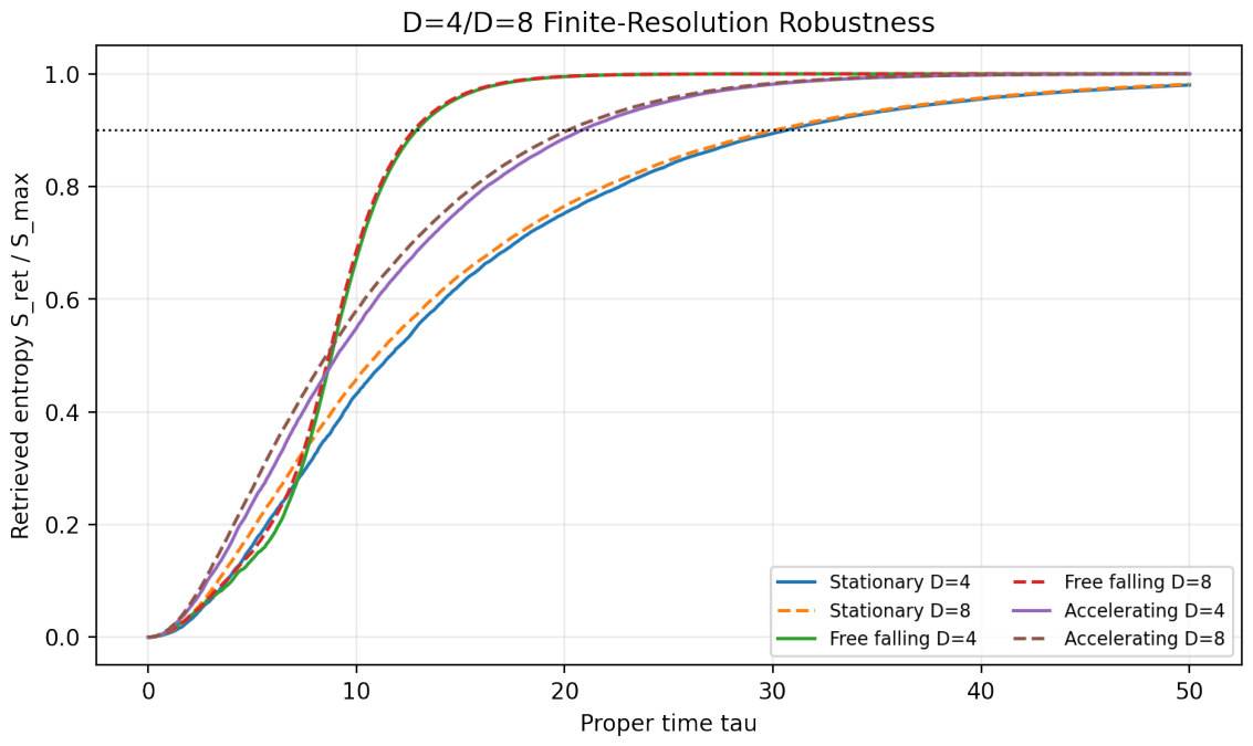
Figure A2.
Synthetic matched-envelope alternatives compared with the accelerating-observer benchmark. Logistic, Gompertz, stretched-exponential, and Hill-type alternatives reproduce the shape of an isolated trajectory after calibration. The comparison therefore evaluates the larger joint specification, including the declared supply, observer protocol, composite-hazard recovery, and correlator map. Observer ordering is benchmark-specific rather than a universal consequence of saturation. The released figure’s axis is the normalized quantity , with when the legacy numerator is identified with .
Figure A2.
Synthetic matched-envelope alternatives compared with the accelerating-observer benchmark. Logistic, Gompertz, stretched-exponential, and Hill-type alternatives reproduce the shape of an isolated trajectory after calibration. The comparison therefore evaluates the larger joint specification, including the declared supply, observer protocol, composite-hazard recovery, and correlator map. Observer ordering is benchmark-specific rather than a universal consequence of saturation. The released figure’s axis is the normalized quantity , with when the legacy numerator is identified with .
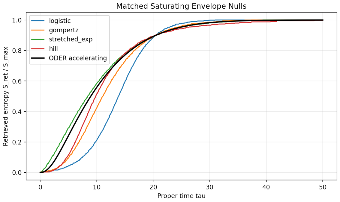
Appendix C.5. Multi-Protocol Overlap Diagnostic and Differential-Acceleration Interferometer
Multi-protocol comparison has two forms: a joint channel yields an information allocation bound, while a declared observation model yields an experimental overlap diagnostic.
For descriptive comparison of two normalized retrieval traces, define
whenever the denominator is nonzero. This scalar records overlap between two normalized retrieval traces. Mutual-information allocation is governed separately by Eq. (99).
A prospective Differential-Acceleration Interferometer can test a preregistered joint observation model. Stationary and accelerated arms are baseline-aligned, each arm measures its local surface, and the analysis estimates the difference between protocol-conditioned envelopes. Thermal drift, switching asymmetry, unequal detector efficiency, and ordinary decoherence enter as explicit controls. A retrieval-specific interpretation requires the measured arm difference to track independently calibrated changes in , , or rather than acceleration alone.
ROC or likelihood comparisons test the declared joint model after the null and alternative families are specified.
Appendix C.6. Phenomenological Retrieval Envelope
The primary observation model used in the synthetic tests is
with and fixed by the baseline decorrelation time. is measured under the null protocol. On the extremal analytic benchmark, is the cosh-power trajectory in Eq. (66). The map is monotone in each retrieval argument for positive .
The model is tested after the baseline, protocol classes, time alignment, and fitting procedure are fixed. In Tier 0B, qualifying archived measurements are reconstructed along registered minimally aggregated and conventional processing paths before the candidate envelope is fitted. When the archive lacks independent estimates of and , that retrospective stage tests operator dependence at the level and does not claim direct inversion of the latent retrieval law. The registered Tier 1 current-platform protocol targets the held-out surface, bandwidth dependence, and matched-null discrimination. Independent activation adds the modular-ratio test. Reference-tagged estimates of add stable recovery and dose composition.
The experimental design adopts millisecond-scale timing and as registration criteria for the power analysis. The selected platform must establish achieved power from its cadence, integration window, and noise model. The comparison also requires controlled protocol classes and the mapping conditions specified in Section 7. The v2 verification artifact contains the implementation of the inversion and verification pipeline, including the generated manifest, report, figures, and CSV tables. The archived scripts are released under an MIT license with pinned dependency specifications for environment replication.
Appendix D. Covariant Retrieval–Curvature Interface and Geometric Response
Appendix D.1. Covariant Source Interface and Controlled Scaling
The fixed-background theorems determine the information-transfer current and its response to supply, activation, and observer lifetime. Completing geometric feedback requires one additional physical object: an observer–field interaction whose metric variation produces a renormalized stress tensor. This subsection states that interface and the conditions that close it.
Let denote the quantum fields and let collect the observer’s admission, memory, and readout degrees of freedom. Introduce a coupling parameter through
After the state and renormalization prescription are fixed, the interaction defines
The coupled semiclassical equation is then
Diffeomorphism invariance requires covariant conservation of the complete right-hand side. Energy transferred between the field and observer sectors therefore appears with equal and opposite exchange currents rather than as an independent source added by hand.
The retrieval theory defines the scalar current along the observer worldline,
It does not identify this dimensionless information current with an energy density. A microscopic realization completes the matching by deriving an energy scale per retrieved reference unit and the spacetime support of the exchange. For example, if is the independently calculated energy per retrieved unit and is the effective proper interaction volume, a local energy-transfer condition may take the form
with the opposite sign assigned to the sector that loses the energy. Equation (A76) is a completion condition, not an identification of information with stress energy: fixes the tensor structure, while and fix the physical conversion.
Let be the curvature radius of the prescribed background over the interaction region . The dimensionless control parameter
separates perturbative feedback, , from a self-consistent strong-backreaction regime. Unlike an estimate built from alone, this quantity can be evaluated once the interaction, renormalization, energy conversion, and support are supplied.
Appendix D.2. Retrieval-Coupled Focusing and Geometric Response
This subsection develops the retrieval–curvature extension in three layers: an exact focusing diagnostic, its specialization to the retrieval law, and the geometric response produced by the covariant source in Appendix D.1. Only the third layer changes the spacetime geometry.
Let generate a timelike geodesic congruence in four spacetime dimensions, with expansion , shear , and vorticity . Its Raychaudhuri equation is
The coefficient is the four-dimensional timelike value. Equation (A78) remains the spacetime focusing law on the prescribed background.
Retrieval-weighted expansion.
Define
where is a constant dimensionless diagnostic weight. This scalar measures geometric expansion together with the local rate at which the observer’s retained reference fraction changes. Substituting into Eq. (A78) gives the exact identity
This first layer is kinematic: it introduces no new stress tensor and changes no fixed-background theorem.
Retrieval-law specialization.
The trajectory in this paper is not an arbitrary differentiable function. Let denote the remaining retrieval gap. The exact continuous law gives
Consequently the order- retrieval contribution in Eq. (187) is
Thus
Because ,
so the modularly constrained activation onset enters the focusing diagnostic through a specific term rather than through an arbitrary second derivative. Supply arrival, kinetic traversal, and activation therefore make separately identifiable contributions to .
Dynamical geometric coupling.
When the covariant interaction in Eq. (A72) is turned on, the source changes the curvature term in Eq. (190). At fixed background tangent, and isolating the direct interaction-source contribution to first order in ,
Worldline variations and induced changes in the background field and observer stress tensors enter as additional linear-response terms. Equation (A83) is the geometric channel absent from the purely kinematic identity: once is specified, retrieval-related energy exchange changes focusing through the semiclassical field equation.
Coupled retrieval-horizon shift.
The same perturbation closes the operational part of the extension. Write
Linearizing gives
For , the solution is
Let be a simple threshold crossing of the uncoupled trajectory, so and . The implicit-function theorem then gives the first-order shift
The horizon shift therefore follows from the response of the actual coupled retrieval solution. The completion chain is explicit: the microscopic interaction determines ; the perturbed geometry determines and ; and Eqs. (195) and (A86) determine the observable horizon shift. Equations (190) and (A86) form the retrieval–curvature program: the information dynamics are explicit, the geometric source is covariant, and the fixed-background limit remains exact.
Appendix E. Split-Property Regularization and the Type III 1 Limit
This appendix separates two structures used in the paper: the split inclusion that provides a Type-I representation of restricted local algebras, and the detector restriction that selects an operational spectral band. They are independent inputs.
Local algebras in continuum AQFT are generically Type III and therefore do not admit an ordinary trace or subsystem density matrix. Mutual information is accordingly defined through Araki relative entropy, as in Eq. (2). A split inclusion permits a regulated density-operator representation without changing that primary definition.
Appendix E.1. Split Inclusion and Operational Spectral Restriction
For nested regions with compactly contained in , assume
where is a Type-I factor and denotes the spatial collar separating the regions [26,27]. Normal states restricted to admit density-operator representations. The factor may remain infinite dimensional, and its modular generator need not be bounded.
The detector protocol is specified separately by its switching, aperture, passband, and readout map. Denote this operational channel by
where b collects the detector settings. A finite passband may define an effective frequency scale or a finite-dimensional resolved sector. That restriction belongs to . Neither bounded spectral support nor a relation follows from the split property.
Appendix E.2. Physical Interpretation
The split distance regulates the algebraic separation between nested regions. Detector resolution is controlled by b. Two protocols may use the same split inclusion and different passbands, or the same passband and different split collars. Keeping these axes distinct prevents a detector cutoff from being mistaken for a property of the continuum modular spectrum.
The retrieved quantity remains
Its value depends on the state, causal restriction, detector channel, and retained memory. The split factor only provides a representation in which the same relative-entropy quantity can be evaluated with density operators.
Appendix E.3. Finite-Resolution Scaling Diagnostic
Resolution scaling is an empirical diagnostic rather than an algebraic theorem. A controlled study should vary the split collar and the detector setting b independently. Stability under changes in tests regulator sensitivity of the restricted information quantity. Changes with test detector-band dependence of the activation and observation maps.
If a detector family has a calibrated bandwidth law , onset curves may be compared after rescaling by . Curve collapse would support that detector model over the tested range. It would not establish a universal relation between the split distance and the modular spectrum.
Appendix E.4. Continuum Completion and Regulator Stability
The continuum-completion program is action oriented:
- 1.
- construct the directed split family and establish the relative-entropy limit as the split collar is reduced;
- 2.
- preserve isotony and locality under compatible embeddings and channels across that directed family;
- 3.
- derive the activation class from a concrete detector-restricted modular observable and establish the conditions required by Eq. (56); and
- 4.
- test the inferred pair under independent regulator and protocol refinement.
These are continuum-completion and regulator-stability conditions. They do not alter the fixed-split theorem proved for a declared Type-I factor and detector channel.
Appendix E.5. Physical Meaning of the Type III 1 Limit
The limit removes the split collar and returns the continuum local-algebra problem. It does not represent infinite detector bandwidth, perfect physical access, or a bounded-to-unbounded spectral transition established by this paper. Detector limits remain encoded in b even when the algebraic regulator is varied.
All finite-observer predictions are stated for declared split representations and declared detector channels. Continuum statements are made through relative entropy and data processing, which do not require a trace or a bounded modular Hamiltonian.
Appendix F. Modular Retrieval in Kerr Geometry: Stationary-Generator Instantiation
This appendix instantiates the observer channel with a stationary Kerr generator. The transfer theorem determines the retrieval dynamics; Kerr geometry fixes the admissible clock, causal domain, and protocol-dependent deformation.
Appendix F.1. Kerr Geometry and the Admissible Generator
For constant angular velocity , define
A stationary observer following this field is admissible only on a region where
On such a region,
is the normalized four-velocity, and proper time satisfies along the orbit. At a null boundary of , this stationary proper-time parameterization ceases to define the observer channel.
Appendix F.2. Conditional Retrieval Channel
Once the state, causal supply, detector protocol, and memory channel are declared, the flagged transfer model gives
Kerr parameters enter through the state-dependent causal supply, detector response, switching clock, and kinetic factor. These inputs determine the geometry-specific instance of Eq. (A89).
The stationary redshift benchmark is
It converts the declared coordinate-time rate into proper time. As approaches null, the stationary clock reaches its domain boundary and the benchmark terminates.
The conversion does not create retrieval by redshift alone. Writing , one has and . Proposition 8 therefore gives
This is the Kerr specialization of the general clock-reparameterization identity. The lapse cancels before the stationary domain boundary is reached. A larger retrieval dose must come from the state, admitted supply, base transition rate, activation, or duration of the admissible protocol.
Appendix F.3. Conditional Analytic Activation
For an independently calibrated Kerr-adapted detector coordinate satisfying the analytic-strip conditions of Section 3.5,
is the equality branch of the activation bound. Kerr stationarity fixes the admissible generator; the analytic detector class fixes the activation profile. Outside that class, the exact flagged transfer law continues with the calibrated activation appropriate to the protocol.
Appendix F.4. Superradiance and Channel Domain
Superradiant mode amplification is frequency, azimuthal-number, state, and frame dependent. It can alter both the supply admitted by the detector and the effective transition rates. A Kerr retrieval instantiation must therefore declare the mode sector and passband before assigning , , or . Where no suitable timelike stationary generator exists, the stationary channel is undefined and a nonstationary trajectory description is required.
Rotating BEC systems emulate azimuthal flow and protocol-dependent spectral response. They test the Kerr-inspired observation and activation maps at the level of those controlled kinematic features.
Appendix F.5. Interpretation and Consequences
The Kerr extension establishes a conditional domain map:
- the remaining-gap structure is inherited from the declared transfer channel;
- the supply and composite hazard depend on through the state, trajectory, and detector protocol;
- the general clock-dose invariance makes lapse cancellation automatic for lapse-only conversion and prevents redshift alone from forcing retrieval near a null boundary;
- the calibrated analytic class determines whether the extremal activation profile survives; and
- the null boundary of terminates the stationary protocol.
The coherent-information supply floor is inherited unchanged: if the Kerr-conditioned protocol satisfies , then no choice of transfer rate or stationary proper-time duration produces a positive-coherent-information horizon for that observer channel.
Appendix G. Interpretive Correspondence
This appendix collects the principal quantities and their gravitational or holographic interpretations. Section 3 fixes the definitions; the correspondences translate them into familiar physical language.
Appendix G.1. Information and Access Quantities
-
Global diary encoding in cumulative radiation:The selected state and radiation model determine it. The radiation entropy Page curve and the diary-encoding curve track distinct quantities.
-
Total reference information in the observer’s causally admitted residual radiation and retained memory:It is the supply ceiling for the exact transfer model and obeys .
-
Normalized retrieved reference information:It measures diary reference information retained in memory. This retrieval quantity sits at a different stage of the recovery chain from both the memory’s marginal entropy and the Bekenstein–Hawking entropy.
-
Coherent information of the flagged memory channel:Its sign changes at . Positive asymptotic quantum capacity follows under the additional independent-memoryless-use interpretation of the erasure channel.
- Operational
- retrieval sectors The retained, admitted-but-unretained, and unavailable outcomes recorded by the observer’s admission-and-readout instrument. Their orthogonality belongs to the output record, not to an assumed block decomposition of the incoming Hawking radiation. Exact branch fidelity and decoupling produce the flagged state; branch errors control its trace-distance approximation.
- The remaining normalized reference information in causally accessible residual radiation for the exact orthogonally flagged state. It is the available transfer gap: admitted diary information still in transit rather than information destroyed by the observer channel.
- E
-
The capture-record register in the unitary dilation. For the exact flagged construction,The record identifies whether capture occurred while remaining blind to the diary content.
- Composite access hazard:where . This is the quantity identified by the retrieval trajectory when is independently known. Under a change of clock it transforms as a rate density, leaving the integrated retrieval dose invariant.
-
The transfer and incoming-supply currents,They obey and . Causal collection changes the admitted budget; observer-local transfer changes its allocation between radiation and memory.
- Kinetic traversal factor in the optional factorization . Independent activation calibration identifies it separately from the composite hazard inferred from . When activation is treated as a scalar trace, carries the corresponding rate-density transformation under a change of clock.
- Protocol-dependent activation, with . The analytic speed limit constrains its onset; the transfer channel gives the remaining-gap factor and the radiation model sets the causal supply.
Appendix G.2. Time, Resolution, and Failure Quantities
- The calibrated onset width of the chosen activation model. Scrambling, Page transition, causal arrival, and total retrieval occur on their own clocks.
- An operational threshold time defined by a declared criterion, such as for a fixed below the admitted terminal supply. It marks a threshold event in the observer protocol; geometric horizons and RT/HRT surfaces mark different events.
-
The first time the flagged memory channel crosses into positive coherent information:Unlike the conventional reporting threshold, this boundary follows from the erasure-channel Choi state. It does not exist when the admitted supply never exceeds one half.
- The first times at which the global diary encoding and the observer’s admitted supply reach the same threshold q. Data processing orders the three clocks as .
-
The proper-time margin between the operational termination time and the retrieval threshold:Its sign is meaningful only when both times use the same observer clock and protocol.
- The spatial collar in a split inclusion . It regulates the algebraic representation. The detector bandwidth is a separate protocol variable.
- Detector settings and, where calibrated, their effective spectral scale. They belong to the observation channel and are independent of the split distance.
Appendix G.3. Holographic and Gravitational Reading
The global encoding curve can be compared with statements about where diary correlations are represented in radiation or a boundary reconstruction wedge. The causal supply asks which part of that encoding enters a declared observer channel. The retrieved fraction asks which part reaches retained memory. This sequence preserves the distinction between representation, causal access, transfer, and decoding.
RT/HRT, islands, causal wedges, and tensor-network codes describe global encoding and reconstructability. An explicit observer channel carries that structure into and the retained record. Redshift, switching, detector response, and state occupation determine the access hazard ; stress tensors, curvature scalars, and geometric lapses remain separate geometric objects.
The complete operational correspondence is
The first arrow is causal admission. The second is a unitary redistribution of diary correlation from radiation to memory with a diary-blind capture record. The admission-and-readout instrument records the corresponding operational sectors without requiring microscopic radiation to be block diagonal. The final marker is the intrinsic coherent-information boundary, and the modular activation theorem bounds the earliest observer time at which it can be crossed.
These correspondences locate the black-hole instantiation without making holography, split regularization, or Kerr stationarity the source of the retrieval law.
References
- Almheiri, A.; Engelhardt, N.; Marolf, D.; Maxfield, H. The Entropy of Bulk Quantum Fields and the Entanglement Wedge of an Evaporating Black Hole. J. High Energy Phys. 2019, 063. [CrossRef]
- Penington, G.; Shenker, S.H.; Stanford, D.; Yang, Z. Replica Wormholes and the Black Hole Interior. J. High Energy Phys. 2022, 205. [arXiv:1911.11977 (hep-th)]. [CrossRef]
- Almheiri, A.; Hartman, T.; Maldacena, J.; Shaghoulian, E.; Tajdini, A. The Entropy of Hawking Radiation. Rev. Mod. Phys. 2021, 93, 035002. [CrossRef]
- Liu, H.; Vardhan, S. Entanglement Entropies of Equilibrated Pure States in Quantum Many-Body Systems and Gravity. PRX Quantum 2021, 2, 010344. [CrossRef]
- Page, D.N. Average Entropy of a Subsystem. Phys. Rev. Lett. 1993, 71, 1291–1294. [CrossRef]
- Hayden, P.; Preskill, J. Black Holes as Mirrors: Quantum Information in Random Subsystems. J. High Energy Phys. 2007, 120. [CrossRef]
- Bennett, C.H.; DiVincenzo, D.P.; Smolin, J.A. Capacities of Quantum Erasure Channels. Phys. Rev. Lett. 1997, 78, 3217–3220. [CrossRef]
- Barnum, H.; Smolin, J.A.; Terhal, B.M. The Quantum Capacity Is Properly Defined without Encodings. Phys. Rev. A 1998, 58, 3496–3501. [CrossRef]
- Choi, M.-D. Completely Positive Linear Maps on Complex Matrices. Linear Algebra Appl. 1975, 10, 285–290. [CrossRef]
- Schumacher, B.; Nielsen, M.A. Quantum Data Processing and Error Correction. Phys. Rev. A 1996, 54, 2629–2635. [CrossRef]
- Gorini, V.; Kossakowski, A.; Sudarshan, E.C.G. Completely Positive Dynamical Semigroups of N-Level Systems. J. Math. Phys. 1976, 17, 821–825. [CrossRef]
- Lindblad, G. On the Generators of Quantum Dynamical Semigroups. Commun. Math. Phys. 1976, 48, 119–130. [CrossRef]
- Attal, S.; Pautrat, Y. From Repeated to Continuous Quantum Interactions. Ann. Henri Poincaré 2006, 7, 59–104. [CrossRef]
- Wootters, W.K.; Zurek, W.H. A Single Quantum Cannot Be Cloned. Nature 1982, 299, 802–803. [CrossRef]
- Akers, C.; Faulkner, T.; Lin, S.; Rath, P. The Page Curve for Reflected Entropy. J. High Energy Phys. 2022, 06, 089. [CrossRef]
- Witten, E. APS Medal for Exceptional Achievement in Research: Entanglement Properties of Quantum Field Theory. Rev. Mod. Phys. 2018, 90, 045003. [CrossRef]
- Chandrasekaran, V.; Longo, R.; Penington, G.; Witten, E. An Algebra of Observables for de Sitter Space. J. High Energy Phys. 2023, 082. [CrossRef]
- Crispino, L.C.B.; Higuchi, A.; Matsas, G.E.A. The Unruh Effect and Its Applications. Rev. Mod. Phys. 2008, 80, 787–838. [CrossRef]
- Steinhauer, J. Observation of Quantum Hawking Radiation and Its Entanglement in an Analogue Black Hole. Nat. Phys. 2016, 12, 959–965. [CrossRef]
- Casini, H.; Huerta, M.; Myers, R.C. Towards a Derivation of Holographic Entanglement Entropy. J. High Energy Phys. 2011, 036. [CrossRef]
- Dong, X.; Harlow, D.; Wall, A.C. Reconstruction of Bulk Operators within the Entanglement Wedge. Phys. Rev. Lett. 2016, 117, 021601. [CrossRef]
- Jafferis, D.L.; Lewkowycz, A.; Maldacena, J.; Suh, S.J. Relative Entropy Equals Bulk Relative Entropy. J. High Energy Phys. 2016, 004. [CrossRef]
- Faulkner, T.; Li, M. Asymptotically Isometric Codes for Holography. arXiv 2022, arXiv:2211.12439 [hep-th]. [CrossRef]
- Pastawski, F.; Yoshida, B.; Harlow, D.; Preskill, J. Holographic Quantum Error-Correcting Codes: Toy Models for the Bulk/Boundary Correspondence. J. High Energy Phys. 2015, 149. [CrossRef]
- Casini, H.; Huerta, M.; Rosabal, J.A. Remarks on Entanglement Entropy for Gauge Fields. Phys. Rev. D 2014, 89, 085012. [CrossRef]
- D’Antoni, C.; Longo, R. Interpolation by Type I Factors and the Flip Automorphism. J. Funct. Anal. 1983, 51, 361–371. [CrossRef]
- Fewster, C.J. The Split Property for Quantum Field Theories in Flat and Curved Spacetimes. Abhandlungen aus dem Mathematischen Seminar der Universität Hamburg 2016, 86, 153–175. [CrossRef]
- Longo, R. Notes on Algebraic Invariants for Noncommutative Dynamical Systems. Commun. Math. Phys. 1979, 69, 195–207. [CrossRef]
- Araki, H. Relative Entropy for States of von Neumann Algebras II. Publ. Res. Inst. Math. Sci. 1977, 13(1), 173–192. [CrossRef]
- Witten, E. Gravity and the Crossed Product. J. High Energy Phys. 2022, 008. [CrossRef]
- Takesaki, M. Tomita’s Theory of Modular Hilbert Algebras and Its Applications. Springer: Berlin, 1970. [CrossRef]
- Maldacena, J.; Susskind, L. Cool Horizons for Entangled Black Holes. Fortschr. Phys. 2013, 61, 781–811. [CrossRef]
- Ryu, S.; Takayanagi, T. Holographic Derivation of Entanglement Entropy from AdS/CFT. Phys. Rev. Lett. 2006, 96, 181602. [CrossRef]
- Hubeny, V.E.; Rangamani, M.; Takayanagi, T. A Covariant Holographic Entanglement Entropy Proposal. J. High Energy Phys. 2007, 062. [CrossRef]
- Martirosyan, G.; Gazo, M.; Etrych, J.; et al. A universal speed limit for spreading of coherence. Nature 2025, 647, 608–612. [CrossRef]
- Cooper III, E. Analytic Speed Limits and Extremal Rigidity for Strip-Holomorphic Monotone Profiles. Preprints 2026, 2026031232, version 2. Available at: https://www.preprints.org/manuscript/202603.1232 DOI: . [CrossRef]
Figure 1.
Synthetic observer-class kinetic profiles . The stationary class implements slowly varying exterior access, the freely falling class implements rapid post-crossing access growth, and the accelerating class implements enhanced acceleration-dependent access. These calibrated benchmark profiles combine with to form the composite hazards .
Figure 1.
Synthetic observer-class kinetic profiles . The stationary class implements slowly varying exterior access, the freely falling class implements rapid post-crossing access growth, and the accelerating class implements enhanced acceleration-dependent access. These calibrated benchmark profiles combine with to form the composite hazards .
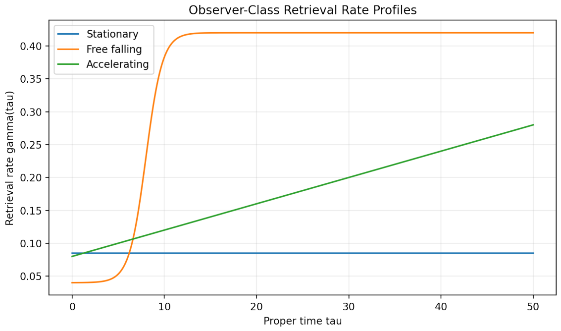
Figure 2.
Synthetic normalized reference retrieval versus observer proper time for stationary, freely falling, and accelerating observer classes. The horizontal dashed line marks the Retrieval Horizon threshold. Shaded regions show confidence bands generated from 200 resampled traces per observer class on an onset-aligned common benchmark comparison clock with the noise model used in the v2 verification artifact. In the legacy vertical-axis label carried by the released figure, identifies the legacy numerator with and uses for this reference-normalized benchmark.
Figure 2.
Synthetic normalized reference retrieval versus observer proper time for stationary, freely falling, and accelerating observer classes. The horizontal dashed line marks the Retrieval Horizon threshold. Shaded regions show confidence bands generated from 200 resampled traces per observer class on an onset-aligned common benchmark comparison clock with the noise model used in the v2 verification artifact. In the legacy vertical-axis label carried by the released figure, identifies the legacy numerator with and uses for this reference-normalized benchmark.
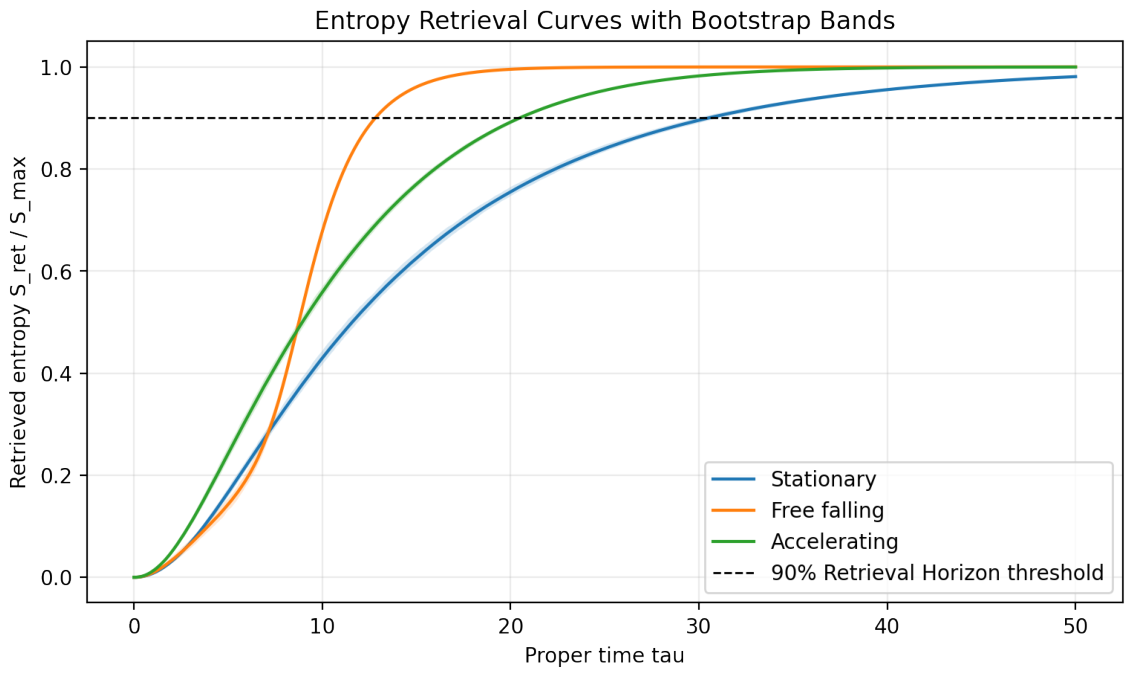
Figure 3.
Synthetic observer-indexed kinetic factors recovered from reference-retrieval traces using independently supplied and the known benchmark activation . The recovered profiles preserve the class-specific structure of the generating rates. This same-trace inversion checks reconstruction; held-out traces test prediction.
Figure 3.
Synthetic observer-indexed kinetic factors recovered from reference-retrieval traces using independently supplied and the known benchmark activation . The recovered profiles preserve the class-specific structure of the generating rates. This same-trace inversion checks reconstruction; held-out traces test prediction.
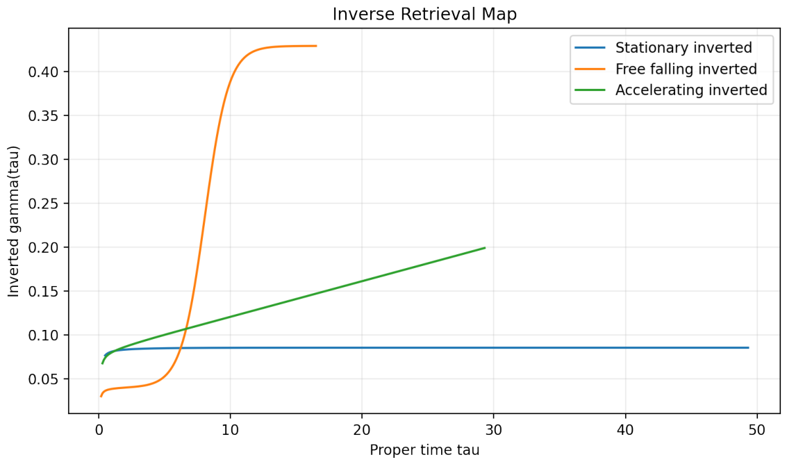
Figure 4.
Synthetic connected-correlation envelope generated from Eqs. (92) and (66) for , , , , , , , and . The diagonal correlation ridge decays as retrieval accumulates, carrying the closed proper-time trajectory into the observable surface.
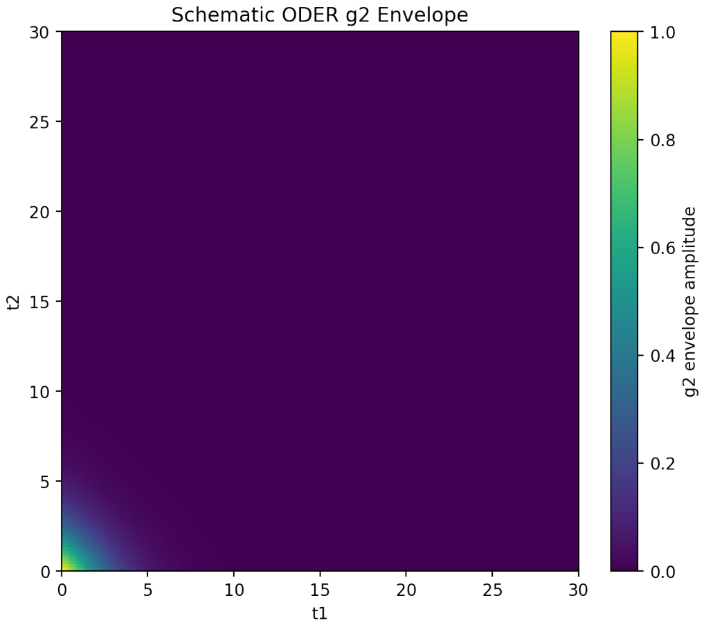
Table 4.
Representative laboratory signatures for each observer class. The entries give the correlation-level behavior generated by each calibrated retrieval-rate profile under the bounded-access model.
Table 4.
Representative laboratory signatures for each observer class. The entries give the correlation-level behavior generated by each calibrated retrieval-rate profile under the bounded-access model.
| Observer | Protocol-dependent input | Correlation signature |
| Stationary | Slowly varying exterior and | Gradual suppression with weak long-range structure |
| Freely falling | Post-crossing change in or | Continuous deformation of the envelope across the crossing |
| Accelerating | Acceleration-conditioned , , and clock | Protocol-conditioned suppression in |
Disclaimer/Publisher’s Note: The statements, opinions and data contained in all publications are solely those of the individual author(s) and contributor(s) and not of MDPI and/or the editor(s). MDPI and/or the editor(s) disclaim responsibility for any injury to people or property resulting from any ideas, methods, instructions or products referred to in the content. |
© 2026 by the authors. Licensee MDPI, Basel, Switzerland. This article is an open access article distributed under the terms and conditions of the Creative Commons Attribution (CC BY) license (http://creativecommons.org/licenses/by/4.0/).
Copyright: This open access article is published under a Creative Commons CC BY 4.0 license, which permit the free download, distribution, and reuse, provided that the author and preprint are cited in any reuse.


