

Submitted:
26 March 2025
Posted:
26 March 2025
You are already at the latest version
Abstract
To address the performance degradation of standard linear extended state observers (LESO) caused by severe peaking phenomena with increasing system order, which compromises controller accuracy, this paper proposes an innovative output feedback controller using a cascaded observer structure. Through the uniform exponential stability (UES) criterion, we demonstrate that the proposed observer guarantees bounded tracking errors for system states. A novel approach constructs desired load pressure from reference trajectories, effectively decoupling the nonlinear interactions between actual load pressure and input signals. By integrating backstepping control methodology with Lyapunov stability analysis, we develop a robust output feedback controller. Extensive simulations validate the proposed controller's effectiveness, extensive simulations validated the effectiveness of the proposed controller, in all four test scenarios, the tracking errors of the proposed controller were reduced by approximately 10% to 61.5% compared to LESO, regarding external disturbance estimation, the estimation accuracy was approximately twice that of LESO.
Keywords:
output feedback controller
; cascaded structure observer
; backstepping control method
; dual valve electro-hydraulic valve
1. Introduction
There are complex and nonlinear characteristics in hydraulic valve control systems, such as compressibility of oil, nonlinear friction, and component wear, which makes it difficult for traditional linear PID control technology to meet modern engineering needs [1]. Therefore, high-performance and reliable control strategies have always been a hot topic in the field of Hydraulic transmission research.
Many nonlinear control methods for electro-hydraulic control systems have emerged over years of development. For example, in reference [2], Guichao Yang et al employed adaptive robust control technology on hydraulic servo actuators to achieve a good position tracking effect and system parameter estimation. In reference [3], Weichao Sun et al applied adaptive robust control technology to achieve vibration suppression of vehicle active suspensions. In reference [4], A Mohanty and B. Yao used indirect adaptive robust control (IARC) technology to improve the tracking accuracy of the robotic arm trajectory. Reference [5,6] used the adaptive backstepping sliding film control method to improve the control accuracy of the electro-hydraulic position servo system. In reference [7], Yang Lin et al. proposed a robust discrete-time sliding mode controller (DT-SMC) for the EHA system, which accurately simulated and compensated the system’s friction characteristics. In reference [8], Q. Guo et al. presented a saturation adaptive control method for the control saturation phenomenon in the motion system of a two-degree-of-freedom robotic arm, achieving satisfactory control performance.
However, the above control methods heavily rely on full-state feedback. Due to cost and structural limitations, many hydraulic transmission systems do not have the conditions to achieve full state observers. Although it is proposed in reference [9] used low-pass filters to process the position information of the research object to obtain velocity and acceleration information, the hysteresis effect caused by filtering and the addition of other noise may cause more serious instability of the system, reducing the control accuracy of the controlled object.
The extended state observer can estimate the immeasurable states in the system, and estimate the parameter uncertainty and external disturbances in the system as concentrated disturbances, weakening the adverse effects of uncertainty factors on the system. In reference [10], researcher Han Jingqing proposed for the first time the Active Disturbance Rejection Control (ADRC) method based on an extended state observer. This control method does not require strict and precise system model parameters, and can achieve corresponding control results by adjusting parameters such as feedback gain and observer bandwidth, and has achieved success in practical applications. References [9,11] all adopt automatic disturbance rejection control technology to achieve precise control of valve-controlled cylinders. In reference [12], L Zhou et al designed a non-integral chain DCMSS control method for servo motors based on a generalized extended state observer (GESO) and verified it in simulation examples. In [13], Wonhee Kim et al designed a feedback control method with a high gain observer and a passive controller, effectively improving the position-tracking performance of the electro-hydraulic system.
However, the self-disturbance rejection control technology is limited by the performance of the extended state observer, and in some cases, the control effect is not satisfactory. Especially the peak phenomenon that occurs during the transient period of the observer can easily induce instability in the feedback control system [14]. In addition, as the order of the system increases, in order to ensure the tracking effect of the high-dimensional state of the system, the observer gain needs to be increased to an exaggerated level [15], which will increase the sensitivity of the system controller to input noise and cause a substantial decline in its stability.
To reduce the impact of the peak phenomenon on controller performance, many scholars have conducted research. In reference [16], Y Huang et al proposed an event-triggering strategy based on output feedback, which ensures real-time boundedness of observation errors by designing reasonable triggering conditions. In [17], M S. Chong et al proposed a hybrid estimation scheme for parameters and states based on multi-state observers. By switching different observers while the excitation conditions persist, the estimation errors of parameters and states converge and are bounded. In [18], Ricardo G. Sanfelice and Laurent Praly proposed an adaptive adjustment algorithm for observer gain, Suppressing the problem of abnormal increase in the observation gain of the system under strong noise or transient conditions. The improved extended state observer proposed in the above research can achieve better estimation performance compared to the standard extended state observer, but it is more complex in structure and increases the difficulty of application in practical engineering.
In reference [19], D Astolfi and L. Marconi proposed a new type of observer, which cascades adjacent system channels in structure. The system state is transmitted through the previous channel to the next level, thus avoiding the problem of the gain of the standard observer falling into an „exponential explosion”. Maopeng Ran et al proposed a new type of extended state observer based on the cascaded first order extended state observer [20], In high-order systems, this observer can limit the peak value of internal variables by adjusting a small number of parameters. More importantly, in terms of structure, this linear extended state observer designed based on a cascaded structure is as concise as the standard extended state observer.
Inspired by reference [19,20], this paper designs a cascaded structure based extended state observer and output feedback controller for a dual spool electro-hydraulic valve control system. Through a large number of simulation examples, it is verified that the proposed controller based on the new observer design has a better performance compared to the standard structure, making it possible to apply it in hydraulic transmission systems.
The main contributions of this paper are summarized below: (1) The proposed output feedback controller obtains unknown system states and external disturbances by constructing a cascaded extended state observer, effectively avoiding the peak phenomenon when the standard extended state observer is applied to high-order systems; (2) In response to the nonlinear coupling phenomenon between the driving pressure and input voltage of the dual valve core electro-hydraulic valve, the expected trajectory of the valve core is used to obtain the expected driving pressure of the valve core to release the coupling relationship and effectively reduce the online calculation burden of the controller.
2. Problem Formulation
This paper focuses on the research of a cascaded structure expansion state observer based on a self-developed dual spool electro-hydraulic valve, as shown in Figure 1.
As shown in Figure 1, the dual valve core electro-hydraulic valve studied in this paper consists of two three-position four-way high-frequency response proportional pilot valves and two three-position three-way main valves. The pilot stage valve core integrates LVDT displacement sensors, which can achieve closed-loop control of the pilot valve displacement. The two main valve cores are the high-pressure valve core and the low-pressure valve core, respectively. The high-pressure valve core is used for oil inlet control and the low-pressure valve core is used for oil return control, thus achieving independent control of the load port. A displacement sensor is installed on the main valve core, and a temperature and pressure sensor is installed in the flow channel between the main valve core and the actuator to sense the oil temperature and load pressure.
Before establishing a nonlinear mathematical model of an electro-hydraulic servo system, this article defines the following parameters.

Table 1.
The parameters used in this paper.
| supply pressure | Return pressure | ||
| Left chamber pressure of the main valve | Main valve right chamber pressure | ||
| Pressure bearing area of the left chamber of the main valve | Pressure bearing area of the right chamber of the main valve | ||
| Main valve core quality | viscous friction coefficient | ||
| Volume of the left chamber of the main valve | Volume of the right chamber of the main valve | ||
| Initial volume of the left chamber of the main valve | Initial volume of the right chamber of the main valve | ||
| Elastic bulk modulus | Main valve core driving force | ||
| Control input voltage | Main valve spring stiffness | ||
| Pilot valve flow coefficient | Hydraulic oil density | ||
| Load flow rate input to the main valve | Pilot valve electrical gain coefficient |
The goal of the controller designed in this article is to achieve high-precision tracking of the expected trajectory of the main valve displacement when only obtaining the displacement and oil supply pressure of the dual spool electro-hydraulic valve. The hydraulic system maintains a constant oil supply pressure of through the accumulator safety valve group, and the oil hydraulic force of in the oil tank is considered zero pressure.
The dynamic model of the main valve core can be described by the following equation
where represents the modeling error including nonlinear friction and the concentrated disturbance caused by external disturbances
The dynamic model of load force at both ends of the main valve core is given by the following equation.
Due to the dual spool valve electro-hydraulic valve system depicted in Figure 1 using a high-frequency response pilot valve as the control input for the main valve, Based on the processing method in reference [9], this paper ignores the dynamic model of the pilot valve and considers it as a proportional relationship between voltage and pilot valve opening, namely, , the load flow rate can be expressed as
where, is the flow gain corresponding to the displacement of the pilot valve core, and is the standard symbol function.
Define the state variable and write the state space equation of the entire system as follows
where
Based on equations (4) and (5), it can be observed that there is a coupling phenomenon between the controller voltage and the load pressure, In subsequent chapters on stability analysis, if load pressure is not measurable, the proof of system stability will not be achieved. Therefore, it is necessary to further study the coupling relationship between voltage and load pressure .
According to the method in [21], the expected load pressure signal can be synthesized based on the expected trajectory and the system dynamics model
By replacing the actual load pressure with the expected load pressure in equation (6), the nonlinear coupling phenomenon between the controller output voltage and load pressure can be relieved. The system state equation can be rewritten as
Where
3. Cascade Observer and Output Feedback Controller Design
3.1. Model Design and Issues to Be Addressed
It should be pointed out that the hydraulic system studied in the article is affected by factors such as oil temperature changes and component wear that are not considered during actual operation, which can lead to changes in system parameters such as and In order to simplify the control scheme, the nominal values of the above physical parameters will be used for subsequent design. The resulting parameter deviations can be considered and concentrated in the system modeling error.
In the following text, an output feedback control strategy will be discussed to overcome internal and external disturbances in the system, so that the valve spool of the main valve follows any smooth expected trajectory as much as possible
The following assumptions run through the entire paper.
Assumption 1:
is much smaller than , which ensures that function is far away from 0.
Assumption 2:
When , is continuously differentiable. At , the left and right derivatives of exist and are bounded, thus ensuring that function satisfies the Lipschitz condition with respect to in the Domain of a function.
Assumption 3:
Function satisfies the Lipschitz condition with respect to in the Domain of a function.
Assumption 4:
The disturbances and exist and are bounded by,.
For the convenience of writing, in the following text, this article will write as; Function writing as ; Write for the function containing observations; And .
3.2. Design of Extended State Observer with Cascade Structure
In this section, an ESO with a cascaded structure will be designed to estimate the unknown state of the system and the concentrated disturbances including modeling errors. The above observed and estimated values will be used to achieve real-time compensation for the controller.
Prior to this, the modeling error in the state space equation needs to be extended to an additional system state variable. The system variable is extended to , and is defined as the derivative of and satisfies the Lipschitz condition. Therefore, the original system state space equation (8) can be rewritten as
Define as the estimated value of system state, where is the estimated value of () and is the state estimated error. Based on the extended system model (10), LESO can be constructed as [20].
where is an internal variable of the system, is an adjustable positive parameter, Parameter is the gain of LESO, which is determined by making Hurwitz polynomial.
Compared with conventional LESO, the designed observer with a new structure has a channel output that is the input of the channel, meaning there is a connection relationship between adjacent channels. In addition, the observer (11) can be seen as a cascade of three first-order extended state observers, effectively reducing the negative impact of high gain coefficients of conventional observers on high-dimensional observation objects.
3.3. Formatting of Mathematical Components
Before proving the convergence of observer (10), some conclusions about time-varying systems need to be cited.
Theorem1:
The following Time-variant system is defined [22].
Lemma1:
Based on Theorem 1, the following generalization can be made for the following Time-variant system
If subsystemsand ,meet the condition of USE, and. ,,。
Then the system (13) is USE.
Lemma2:
For the following Time-variant system
Assume that the linear Time-variant system satisfies the USE condition, and for some normal numbers and integer that are independent of and satisfy , then for and , both make the solution of system (20) satisfy for and .
The following assumption is necessary to prove the convergence of the observer and is reasonable.
Assumption 5:
Function is an n-order differentiable, and there are constants independent of that satisfy inequalities and such thatand
Define
Assumption 6:
The control input and system state are bounded.
Considering the uncertain nonlinear system (10) and the proposed observer (11), under the condition that the above assumptions 1-5 are satisfied and the observer is a compact subset of at the initial time, the following conclusions can be obtained: for and , both make satisfy the following equation
Proof:
In this article, the convergence of
observation errors will be achieved by sequentially converging each order of
error. Because assuming 1-6 is satisfied, it is easy to obtain that each order
state in the system is bounded, and each stage of observer (10) is a stable
system. Therefore, the existence of to is guaranteed.
Define error vector
For the convenience of subsequent proof, define
Step 1: The derivative of can be represented by the following equation
Note that the above equation belongs to the form of system (20), and it is known that and are bounded. Through Lemma 2, it is known that there exists for , , , and to satisfy any , which is equivalent to the case of in (17).
Step 2: The derivative of can be represented by the following equation
According to the definition of error vector , considering equations (19) and (20), the derivative of can be written as
where
It should be pointed out thatis reversible for, and by defining , the following equation can be easily obtained
According to the results of step1, for , the second and third items on the right side of equation (24) are in the form of O (). Combining Lemma 1 and Lemma 2, it can be confirmed that the derivative of is in the form of parameter m = 2 in system (17).
Therefore, it can be concluded that for and , there exists that satisfies for any . On the other hand, can write as
where
So it can be concluded that for , there exists a case where satisfies for any , which is equivalent to the case of in (16).
Step (3): The derivative of can be represented by the following equation
Since functions and satisfy the Lipschitz condition with respect to in the Domain of a function, there exists a constant c1 that satisfies
By assuming 4 and 6, it can be seen that the constraints imposed on ,, and are independent of . Based on the boundedness of , , and , the above equations belong to the form of system (10). Therefore, through Lemma 2, it can be concluded that for , there exists a case where satisfies for any , which is equivalent to the case of in (16).
In summary, the estimation errors of each order system state of observer (10) are bounded, and the observer parameters can be adjusted to minimize the observation error.
3.4. Design of Output Feedback Controller
Step (1): Define an error variable as follows
where is the tracking error of the system output position, is the virtual control rate of the system state , and represents the difference.
From equation (25), it can be seen that due to the inclusion of unknown state , signal in the controller is not measurable. Therefore, needs to be divided into computable and uncomputable parts . is calculated by obtaining through observer (15) and used for subsequent controller design.
Based on equations (10) and (29), the derivative of can be expressed as
Based on the design concept of the backstepping method, is considered as the virtual control input of the system. Next, the control law will be designed to ensure the control performance of the system.
By defining as the control error of the virtual control input and incorporating equation (31), the following equation can be obtained
Based on the state estimation obtained from observer (15), equation (32) yields the virtual control rate as
where, is the model-based compensation term, is the Robust control term to achieve local stability of the system, and is the feedback gain.
By incorporating equation (29) into equation (33), can be reconstructed as
By differentiating from equations (10) and (33), it can be obtained that
where, α2c is the
differentiable part in , and B is the non differentiable part in
The actual input of the system can be synthesized through the online state estimation values of the observer
where, represents the feedback gain, represents the model compensation term obtained from the estimated state, and is the robust feedback term used to stabilize the system.
By incorporating equation (33) into (31), can be reconstructed as
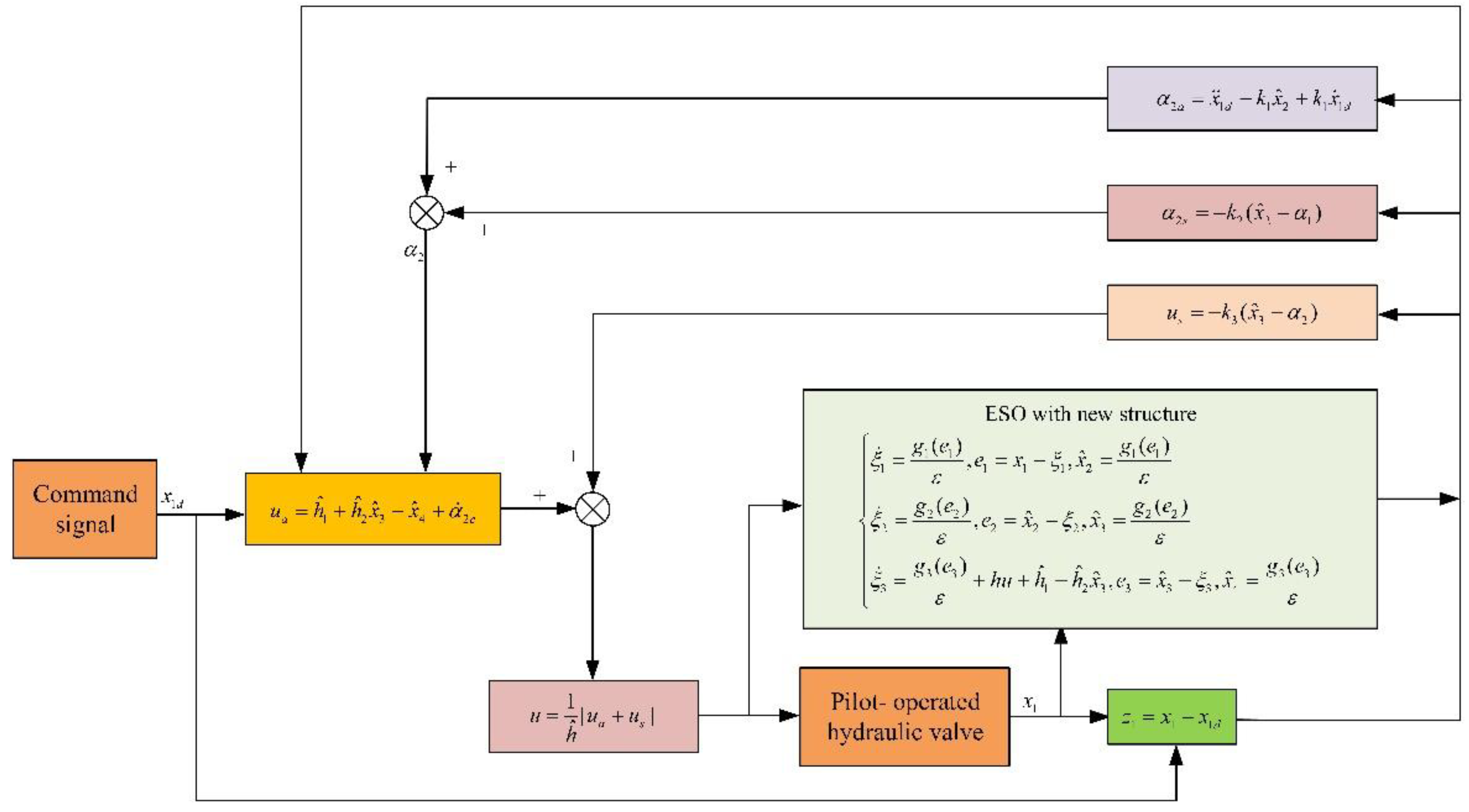
The overall framework of the controller is as follows
Figure 2.
Schematic diagram of controller structure.
3.5. Proof of Convergence of Backstepping Controller
In this section, it will be proven that the backstepping controller mentioned above can make all error signals bounded when used in the system described in this article. Prior to this, additional explanations need to be provided for the observer’s error (10)
Define error vector
According to equations (19), (20), and (27), can be rewritten as
According to the definition of error vector , combined with equations (19), (21), and (39), the derivative of can be written as
where
Since the parameter is determined by making satisfy Hurwitz polynomial, it is easy to obtain that is the Hurwitz matrix, that is, there is a positive definite Symmetric matrix A satisfying
where is a third-order Identity matrix.
The Positive-definite matrix is defined as follows
By differentiating equation (43) and substituting it into equations (34), (38), (40), and (42), it can be obtained that
By assuming the definitions of 2, 3, 6, and, there exists a normal number that satisfies
Define a variable
By assuming 2, 3, and 6, it can be obtained that the existence of a normal number satisfies the inequality
Define a set of known constants
Considering (47) and (48), it can be concluded that
where
Select appropriate control parameters , , , to make the matrix a positive definite matrix, and then obtain
By integrating equation (51), it can be obtained that
Therefore, the tracking error of the system for the expected trajectory is bounded
4. Application Verification
To verify the advantages of the output feedback controller mentioned above, a simulation model of a dual spool electro-hydraulic valve is established. The physical parameters used in the model are shown in Table 2.
In this article, three control schemes are compared, among which control scheme 1 is an output feedback controller designed based on a cascaded linear extended state observer, control scheme 2 is an output feedback controller designed based on a standard structure linear extended state observer, and control scheme 3 is a high gain PID controller. The specific parameter settings are shown in Table 3.
Case1: Given the external disturbance signal, given the valve core position command signal is.
The tracking performance comparison of three controllers applied to the valve core position is shown in Figure 3. The simulation results depict that the tracking error of the backstepping control based on the system model is significantly smaller than that of the high-gain PID control, for the C3 controller, the tracking error is within approximately 40%, for the C2 controller, the control error is within about 13%, for the C1 controller, the control error is within roughly 5%. Compared with controller C2 designed based on the standard LESO, controller C1 designed in this paper based on the cascaded structure observer has a better tracking effect on the position of the valve core.
The comparison of the estimation effects of the two observers for the given external disturbance is collected in Figure 4. The simulation results show that, under the condition of approximate parameters, the estimation effects of the two observers for external disturbances are similar, and both observers can achieve low lag tracking for external disturbances. According to the estimation error reflected in Figure 4 , Subfigure b, the estimation error of external disturbance for C1 is within approximately 1.5%, for C2, the estimation error of external disturbance is within about 3.5%, it can be found that due to the cascade structure, the observer used in C1 has higher estimation accuracy for external disturbances, This also explains that under the same controller parameters, the control error of C1 is smaller.
Case2: The given valve core position command signal is a triangular wave with a cycle of 5 seconds and a stroke of 0-6mm, and given the external disturbance signal is.
Given a triangular wave command for the position of the valve core, the comparison of tracking effects using three different controllers is found in Figure 5. The simulation results present that the tracking errors of the two controllers C1 and C2 based on backstepping control design are significantly smaller than those of the high gain PID controller C3, for the C3 controller, the tracking error is within approximately 7.5%, for the C2 controller, the control error is within about 1.5%, for the C1 controller, the control error is within roughly 0.8%. Compared with controller C2 designed based on the standard LESO, controller C1 designed in this paper based on a cascaded structure observer has better tracking performance when faced with speed changes in triangular wave instructions.
The comparison of the estimation performance of the two observers for a given external disturbance is collected in Figure 6. The simulation results show that both observers can achieve good tracking performance for external disturbances and approximate parameters, and the tracking lag of the two observers for external disturbances is almost invisible. According to the estimation error reflected in Figure 6, Subfigure b, the estimation error of external disturbance for C1 is within approximately 25%, for C2, the estimation error of external disturbance is within about 50%, it can be observed that due to the cascade structure, the observer used in C1 has a smaller estimation accuracy error for external disturbances, which also explains that under the same controller parameters and position instructions, the control error of C1 is smaller.
Case3: The given valve core position command signal is and given the external disturbance signal is.
The position of the valve core is given a sine signal with a cycle of 4 seconds and a stroke of 6mm. The comparison of tracking effects using three different controllers is found in Figure 7. The simulation results depict that the tracking errors of the two controllers C1 and C2 based on backstepping control design are significantly smaller than those of the high gain PID controller C3, for the C3 controller, the tracking error is within approximately 10%, for the C2 controller, the control error is within about 3.5%, for the C1 controller, the control error is within roughly 2.5%. Compared with controller C2 designed based on standard LESO, controller C1 designed in this paper based on cascaded structure observer has better tracking performance when faced with speed sudden changes in triangular wave instructions.
The comparison of the estimation performance of the two observers for a given external disturbance is collected in Figure 8. The simulation results show that both observers can achieve good tracking performance for external disturbances and approximate parameters, and the tracking lag of the two observers for external disturbances is almost invisible. According to the estimation error reflected in Figure 8, Subfigure b, the estimation error of external disturbance for C1 is within approximately 14.5%, for C2, the estimation error of external disturbance is within about 27%, it can be observed that due to the cascade structure, the observer used in C1 has a smaller estimation accuracy error for external disturbances, which also explains that under the same controller parameters and position instructions, the control error of C1 is smaller.
Case4: The given external disturbance signal is, and the given valve core position command signal is
Provide a step signal to the valve core as collected in Figure 9, Subfigure a; the tracking effects of three different controllers are compared as found in Figure 9, Subfigure b; and the tracking error comparison is shown in Figure 9, Subfigure c. The simulation results show that the two controllers C1 and C2 based on backstepping control design will have significant tracking errors when facing severe mismatches in position states, for the C1 controller, the control error is within about 12%, for the C2 controller, the control error is within roughly 13.3%, compared to the controller C2 based on standard LESO design, The controller C1 designed in this article based on a cascaded structure observer has a smaller tracking error, while the high gain PID controller C3 does not show any position mutation through the high gain coefficient. However, through Figure 9, Subfigure b, it can be observed that the entire system is in an unstable working state.
The comparison of the estimation performance of the two observers for a given external disturbance is depicted in Figure 10. The simulation results indicate that under the condition of approximate parameters, both observers can achieve good tracking performance for external disturbances. According to the estimation error reflected in Figure 10, Subfigure b, the estimation error of external disturbance for C1 is within approximately 15%, for C2, the estimation error of external disturbance is within about 38%, it can be observed that due to the cascade structure, the observer used in C1 has a smaller estimation accuracy error for external disturbances, which also explains that under the same controller parameters and position instructions, the control error of C1 is smaller.
5. Conclusions
In this paper, based on the structure and working principle of a dual spool electro-hydraulic valve, a linear extended state observer based on a cascade structure is designed. The expected load pressure is synthesized through the expected trajectory, achieving the decoupling of nonlinear coupling phenomena in the state space equation. On this basis, an output feedback controller is designed based on the backstepping idea. From the stability criterion of Uniform Exponential Stability (USE), it can be seen that the estimation error of the system state for this cascaded observer is convergent. Through the Lyapunov quadratic function and its derivatives, it is proved that the tracking error of the controller designed with this observer for the instruction signal is bounded and convergent. Finally, through extensive simulation case comparisons, in all four working condition tests for spool position tracking performance, C1 achieved tracking errors of 5%, 0.8%, 2.5%, and 12%, C2 recorded errors of 13%, 1.5%, 3.5%, and 13.3%, and C3 demonstrated tracking errors of 40%, 7.5%, 10% with unstable operation. Controllers C1 and C2 designed with backstepping control exhibited significantly smaller tracking errors than controller C3 based on high-gain PID control. In external disturbance estimation tests, C1 achieved estimation errors of 1.5%, 25%, 14.5%, and 15%, while C2 recorded errors of 3.5%, 50%, 27%, and 38%. Due to its cascaded structure, C1 achieved over twice the estimation accuracy of C2 for external disturbances, validating the performance of the designed observer and controllers in this paper. Our future research direction is to combine this new structural observer with methods such as state constraints and adaptive control.
Author Contributions
Methodology, C.J., C.A., Z.Y., and Y.J.; software, H.M.; investigation, S.L., and T.M.; writing—original draft, S.L. writing—review and editing, C.J., C.A., X.K., and Z.Y. All authors have read and agreed to the published version of the manuscript.
Funding
This work was supported by the National Natural Science Foundation of China (grant no. 52175065) and the National Natural Science Foundation of China – Regional Innovation and Development Joint Fund (grant no. U22A20178).
Data Availability Statement
The data are contained within the article..
Conflicts of Interest
Author Cunde Jia and Author Zhuowei Yu are employed by the company Beijing Sany Intelligent Manufacturing Technology Co., Ltd.. The remaining authors declare that the research was conducted in the absence of any commercial or financial relationships that could be construed as a potential conflict of interest..
Abbreviations
| LESO | Linear extended state observer |
| USE | Uniform exponential stability |
| IARC | Indirect adaptive robust control |
| DT-SMC | Discrete-time sliding mode controller |
| ADRC | Active Disturbance Rejection Control |
| GESO | Generalized extended state observer |
| DCMSS | Disturbance Compensation Motion Control System for Servo Motors |
| LVDT | Linear variable differential transformer |
| ESO | Extended state observer |
| supply pressure | |
| Left chamber pressure of the main valve | |
| Pressure bearing area of the left chamber of the main valve | |
| Main valve core quality | |
| Volume of the left chamber of the main valve | |
| Initial volume of the left chamber of the main valve | |
| Elastic bulk modulus | |
| Control input voltage | |
| Pilot valve flow coefficient | |
| Load flow rate input to the main valve | |
| Return pressure | |
| Main valve right chamber pressure | |
| Pressure bearing area of the right chamber of the main valve | |
| viscous friction coefficient | |
| Volume of the right chamber of the main valve | |
| Initial volume of the right chamber of the main valve | |
| Main valve core driving force | |
| Main valve spring stiffness | |
| Hydraulic oil density | |
| Pilot valve electrical gain coefficient | |
| Represents the modeling error including nonlinear friction and the concentrated disturbance caused by external disturbances | |
| System load force modeling error | |
| State variable | |
| Flow gain corresponding to the displacement of the pilot valve core, | |
| Expected load pressure signal | |
| Define error vector | |
| System modeling error | |
| State-transition matrix of the system | |
| Disturbance in the system | |
| Hurwitz matrix | |
| Positive-definite matrix |
References
- B. Yao, F. Bu, J. Reedy and G. T. C. Chiu, „Adaptive robust motion control of single-rod hydraulic actuators: Theory and experiments,” Proceedings of the 1999 American Control Conference (Cat. No. 99CH36251), San Diego, CA, USA, 1999, pp. 759-763 vol.2. [CrossRef]
- C. Guan and S. Pan, „Nonlinear Adaptive Robust Control of Single-Rod Electro-Hydraulic Actuator With Unknown Nonlinear Parameters,” in IEEE Transactions on Control Systems Technology, vol. 16, no. 3, pp. 434-445, May 2008. [CrossRef]
- W. Sun, H. Gao and B. Yao, „Adaptive Robust Vibration Control of Full-Car Active Suspensions With Electrohydraulic Actuators,” in IEEE Transactions on Control Systems Technology, vol. 21, no. 6, pp. 2417-2422, Nov. 2013. [CrossRef]
- A. Mohanty and B. Yao, „Indirect Adaptive Robust Control of Hydraulic Manipulators With Accurate Parameter Estimates,” in IEEE Transactions on Control Systems Technology, vol. 19, no. 3, pp. 567-575, May 2011. [CrossRef]
- Y. Wei, L. Qian, S. Nie and Q. Yin, „Adaptive Backstepping Sliding Mode Control for Electro-hydraulic Position Servo System of The Artillery Projectile Transfer Arm,” 2019 IEEE 4th Advanced Information Technology, Electronic and Automation Control Conference (IAEAC), Chengdu, China, 2019, pp. 893-898. [CrossRef]
- Y. Lin, Y. Shi and R. Burton, „Modeling and Robust Discrete-Time Sliding-Mode Control Design for a Fluid Power Electrohydraulic Actuator (EHA) System,” in IEEE/ASME Transactions on Mechatronics, vol. 18, no. 1, pp. 1-10, Feb. 2013. [CrossRef]
- Fang Yiming, Jiao Zongxia, Wang Wenbin, et al. Adaptive backstepping sliding mode control for hydraulic servo position systems of rolling mills [J]. Journal of Electrical Machinery and Control,2011,15(10):95-10. [CrossRef]
- Q. Guo, J. Yin, T. Yu and D. Jiang, „Saturated Adaptive Control of an Electrohydraulic Actuator with Parametric Uncertainty and Load Disturbance,” in IEEE Transactions on Industrial Electronics, vol. 64, no. 10, pp. 7930-7941, Oct. 2017. [CrossRef]
- Guichao Yang, Jianyong Yao, „Output feedback control of electro-hydraulic servo actuators with matched and mismatched disturbances rejection, „Journal of the Franklin Institute, vol 356, Issue 16,2019. [CrossRef]
- Han J. From PID to Active Disturbance Rejection Control[J]. IEEE Transactions on Industrial Electronics,2009,56(3).
- J. Yao, Z. Jiao, D. Ma, Extended-state-observer-based output feedback nonlinear robust control of hydraulic systems with backstepping, IEEE Trans. Ind. Electron. 61 (11) (2014) 6285–6293.
- L. Zhou, L. Cheng, C. Pan and Z. Jiang, „Generalized Extended State Observer Based Speed Control for DC Motor Servo System,” 2018 37th Chinese Control Conference (CCC), Wuhan, China, 2018, pp. 221-226. [CrossRef]
- Kim W,Won D,Shin D, et al. Output feedback nonlinear control for electro-hydraulic systems[J]. Mechatronics,2012,22(6).
- E. H. El Yaagoubi, A. El Assoudi and H. Hammouri, „High gain observer: attenuation of the peak phenomena,” Proceedings of the 2004 American Control Conference, Boston, MA, USA, 2004, pp. 4393-4397 vol.5. [CrossRef]
- H. K. Khalil, „High-Gain Observers in Feedback Control: Application to Permanent Magnet Synchronous Motors,” in IEEE Control Systems Magazine, vol. 37, no. 3, pp. 25-41, June 2017. [CrossRef]
- Y. Huang, J. Wang, D. Shi, J. Wu and L. Shi, „Event-Triggered Sampled-Data Control: An Active Disturbance Rejection Approach,” in IEEE/ASME Transactions on Mechatronics, vol. 24, no. 5, pp. 2052-2063, Oct. 2019. [CrossRef]
- M. S. Chong, D. Nešić, R. Postoyan and L. Kuhlmann, „Parameter and State Estimation of Nonlinear Systems Using a Multi-Observer Under the Supervisory Framework,” in IEEE Transactions on Automatic Control, vol. 60, no. 9, pp. 2336-2349, Sept. 2015. [CrossRef]
- Ricardo G. Sanfelice, Laurent Praly, „On the performance of high-gain observers with gain adaptation under measurement noise, „Automatica, vol 47, Issue 10,201. [CrossRef]
- D. Astolfi and L. Marconi, „A High-Gain Nonlinear Observer With Limited Gain Power,” in IEEE Transactions on Automatic Control, vol. 60, no. 11, pp. 3059-3064, Nov. 2015. [CrossRef]
- Maopeng Ran, Juncheng Li, Lihua Xie, „A new extended state observer for uncertain nonlinear systems,” Automatica, vol 131, 2021,109772. [CrossRef]
- Ziying Lin, Jianyong Yao, Wenxiang Deng, „Input constraint control for hydraulic systems with asymptotic tracking, „ ISA Transactions, Volume 129, Part A,2022,Pages 616-627, ISSN 0019-0578. [CrossRef]
- Rugh, W. J. 1996. Linear System Theory (2nd ed.). Upper Saddle River, New Jersey: Prentice Hall.
Figure 1.
Structure/Hydraulic Principle of Double Valve Core Electrohydraulic Valve.
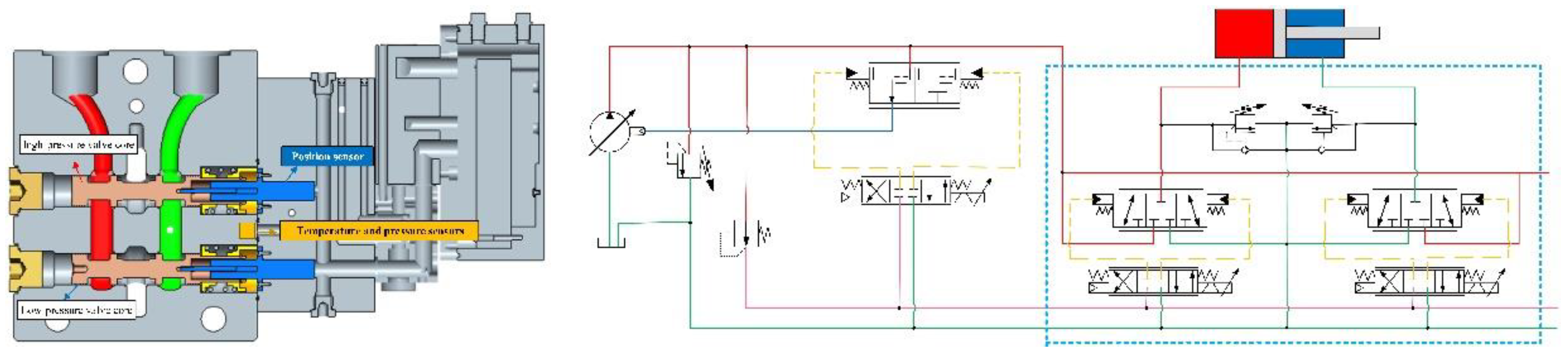
Figure 3.
Comparative Analysis of Position Tracking Performance of Three Controllers. (a) Position tracking effects of three different controllers. (b) Position tracking error of three different controllers.
Figure 3.
Comparative Analysis of Position Tracking Performance of Three Controllers. (a) Position tracking effects of three different controllers. (b) Position tracking error of three different controllers.
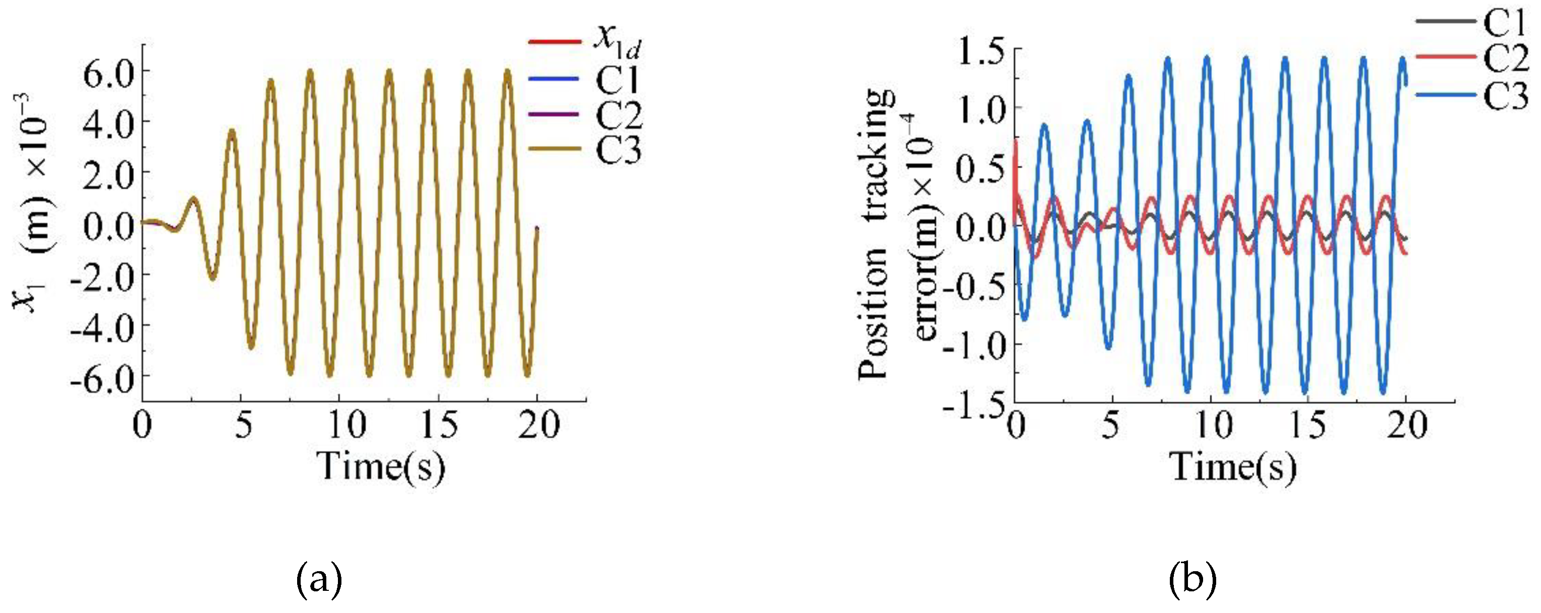
Figure 4.
Estimation of External Disturbances and Error Comparative Analysis by Two Observers. (a) Estimation of External Disturbance for Two Types of Observers. (b) Estimation errors of two types of observers for external disturbances.
Figure 4.
Estimation of External Disturbances and Error Comparative Analysis by Two Observers. (a) Estimation of External Disturbance for Two Types of Observers. (b) Estimation errors of two types of observers for external disturbances.
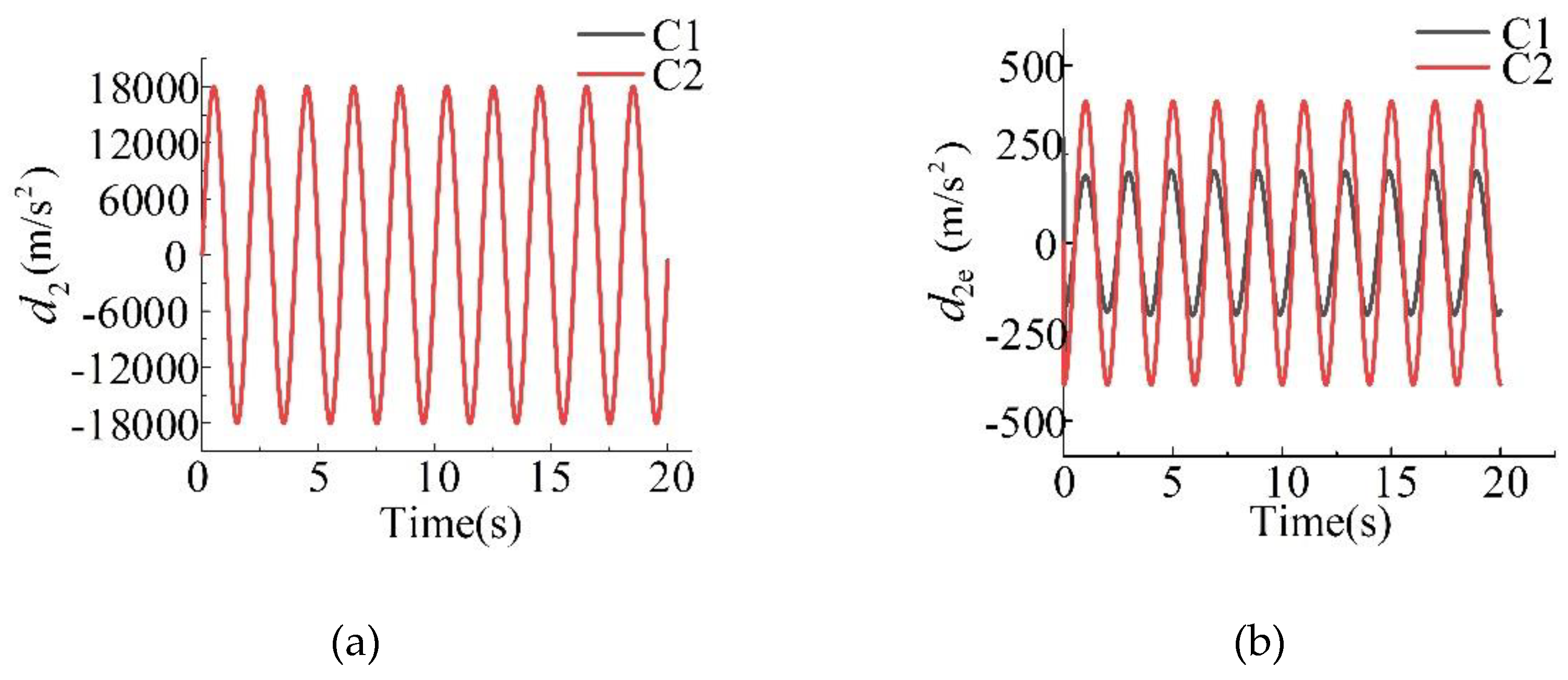
Figure 5.
Comparison of Position Tracking Performance of Three Controllers: Error Characteristics Analysis. (a) Position tracking effects of three different controllers. (b) Position tracking error of three different controllers.
Figure 5.
Comparison of Position Tracking Performance of Three Controllers: Error Characteristics Analysis. (a) Position tracking effects of three different controllers. (b) Position tracking error of three different controllers.
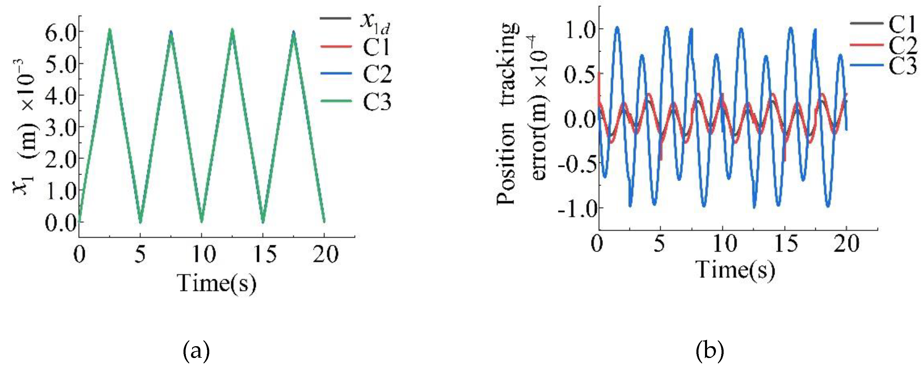
Figure 6.
Comparison of External Disturbance Estimation and Error Analysis for Two Observers. (a) Estimation of External Disturbance for Two Types of Observers. (b) Estimation errors of two types of observers for external disturbances.
Figure 6.
Comparison of External Disturbance Estimation and Error Analysis for Two Observers. (a) Estimation of External Disturbance for Two Types of Observers. (b) Estimation errors of two types of observers for external disturbances.
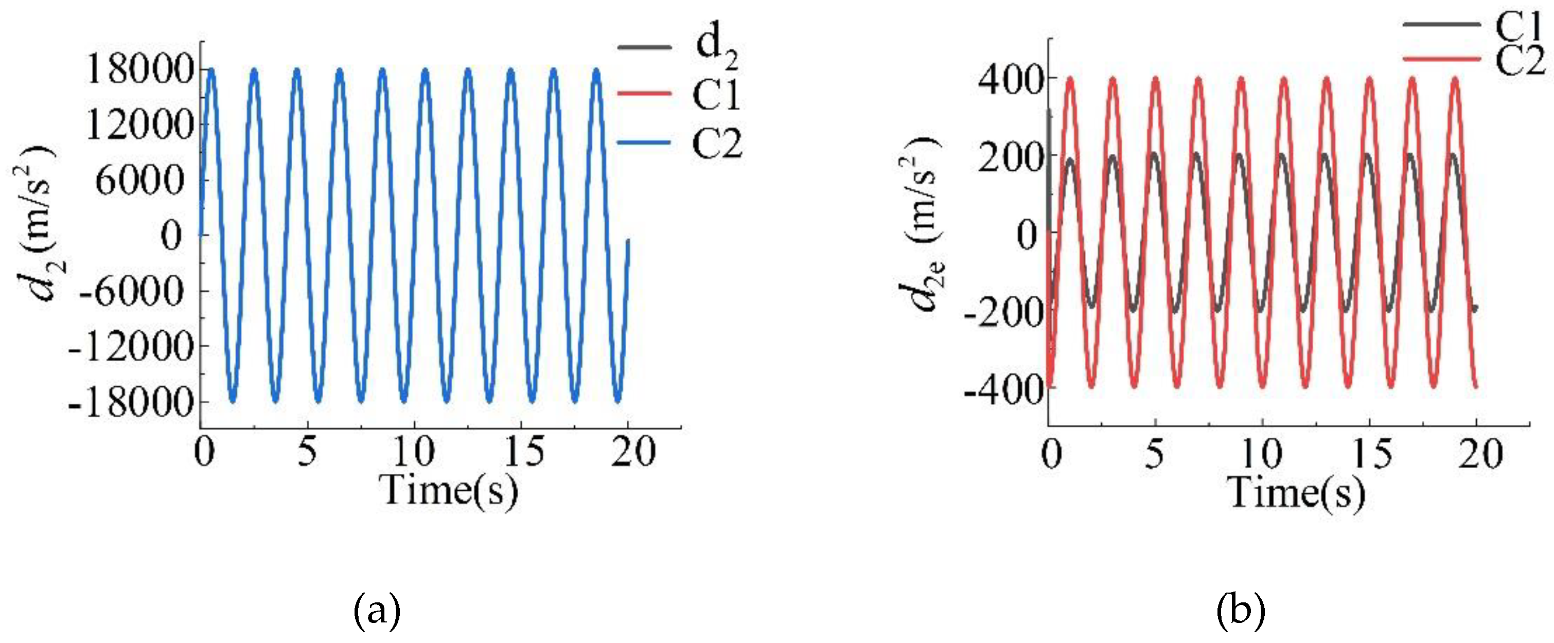
Figure 7.
Comparison of Position Tracking Performance and Error Characteristics Analysis for Three Controllers. (a) Position tracking effects of three different controllers. (b) Position tracking errors of three different controllers.
Figure 7.
Comparison of Position Tracking Performance and Error Characteristics Analysis for Three Controllers. (a) Position tracking effects of three different controllers. (b) Position tracking errors of three different controllers.
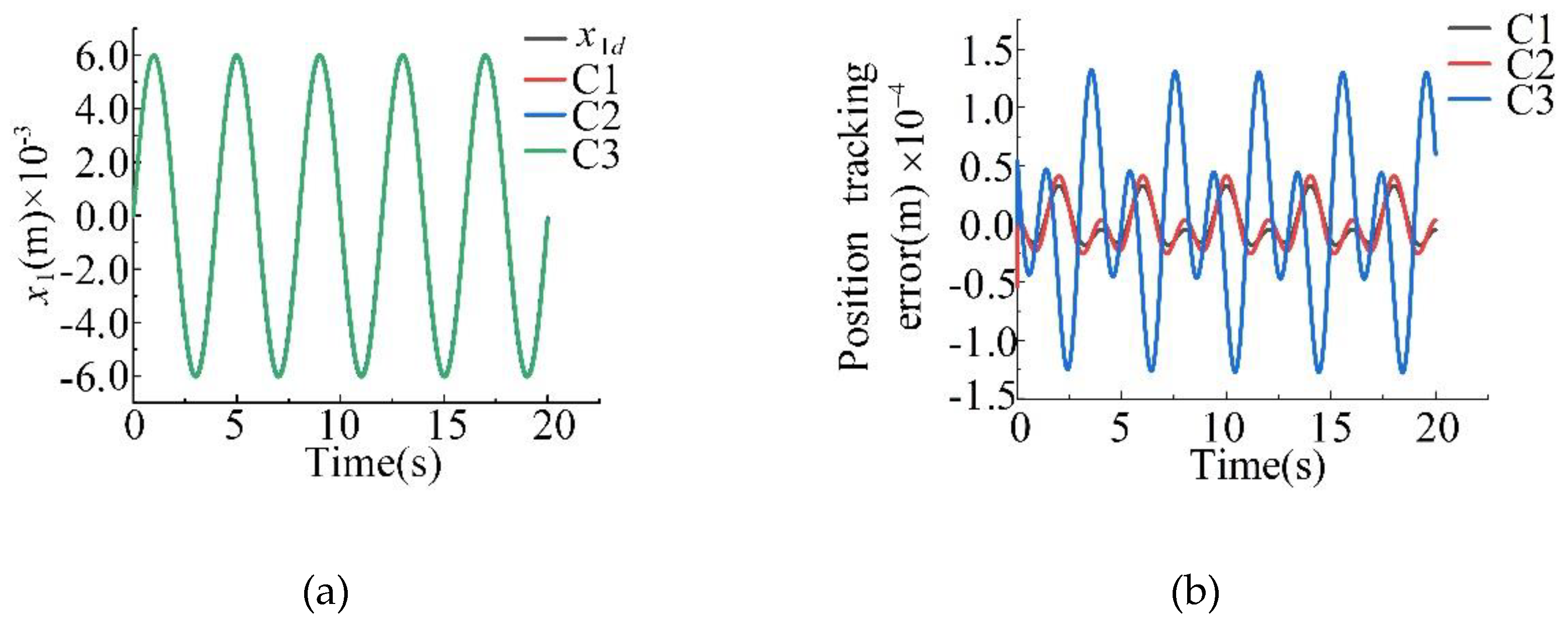
Figure 8.
Comparison of External Disturbance Estimation and Error Analysis for Two Observers. (a) Estimation of External Disturbance by Two Types of Observers. (b) Estimation errors of two types of observers for external disturbances.
Figure 8.
Comparison of External Disturbance Estimation and Error Analysis for Two Observers. (a) Estimation of External Disturbance by Two Types of Observers. (b) Estimation errors of two types of observers for external disturbances.
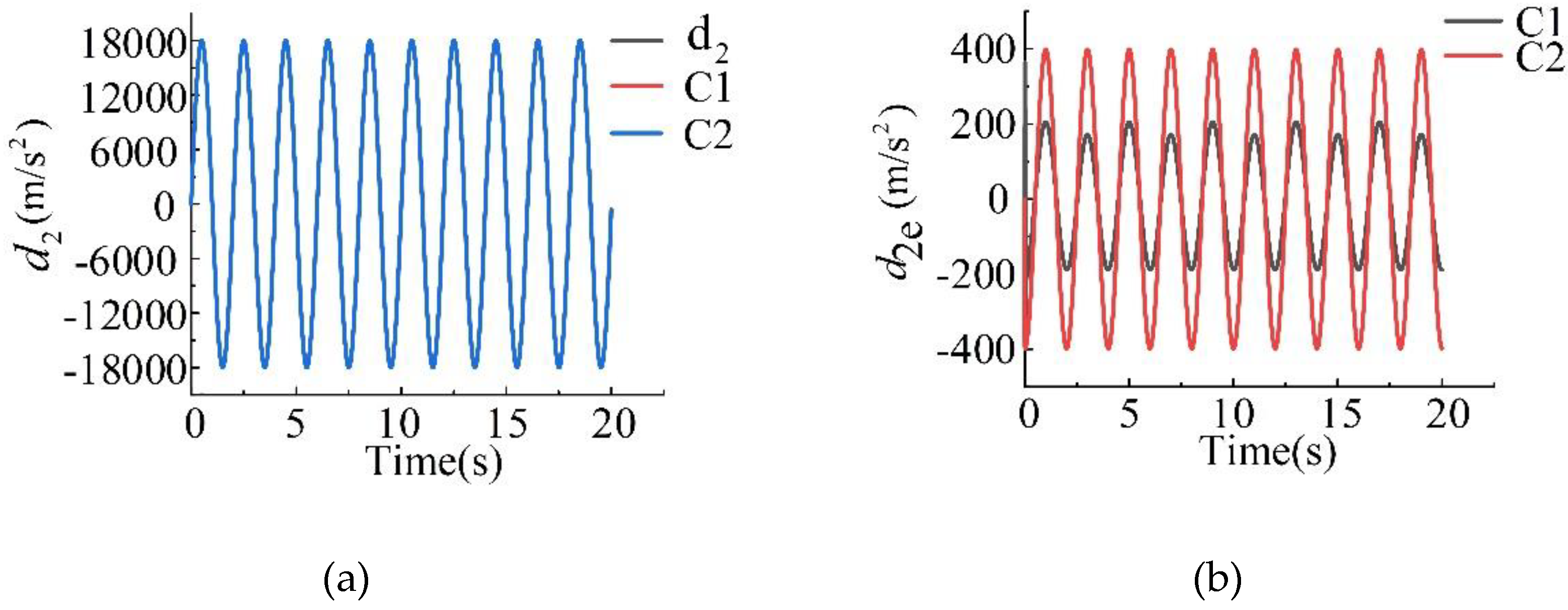
Figure 9.
Comparison of Position Tracking Performance and Error Characteristics Analysis for Three Controllers. (a) Position tracking effects of three different controllers. (b) Partial Enlarged View of Tracking Effect. (c) Position tracking error of three different controllers.
Figure 9.
Comparison of Position Tracking Performance and Error Characteristics Analysis for Three Controllers. (a) Position tracking effects of three different controllers. (b) Partial Enlarged View of Tracking Effect. (c) Position tracking error of three different controllers.
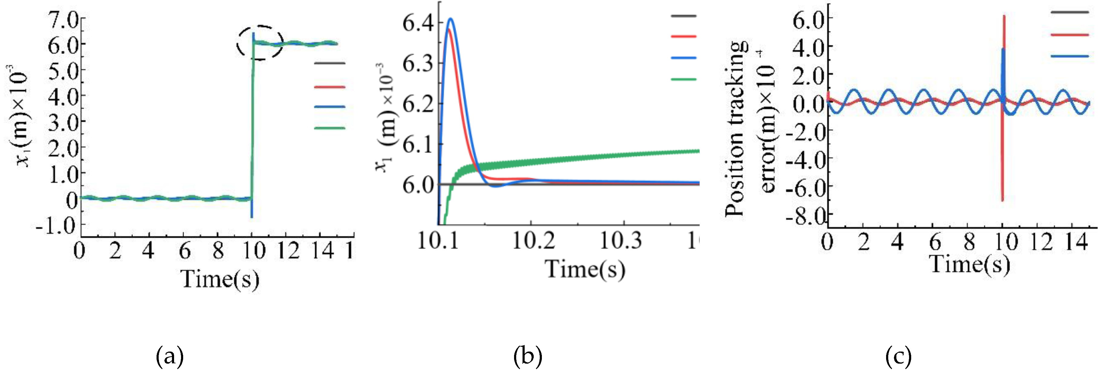
Figure 10.
Comparison of External Disturbance Estimation and Error Analysis for Two Observers. (a) Estimation of external disturbances using two types of observers. (b) Estimation errors of two types of observers for external disturbances.
Figure 10.
Comparison of External Disturbance Estimation and Error Analysis for Two Observers. (a) Estimation of external disturbances using two types of observers. (b) Estimation errors of two types of observers for external disturbances.
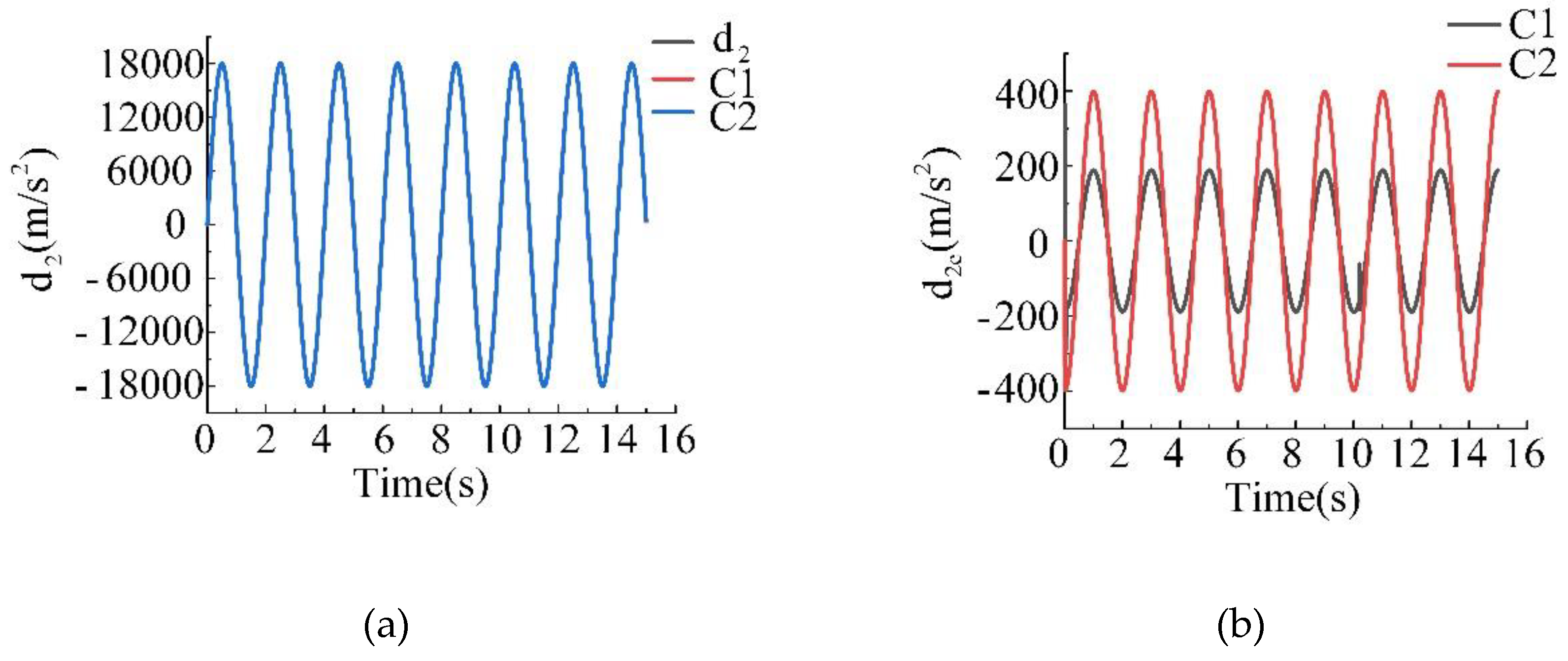
Table 2.
Parameters used in simulation models.
| (kg) | 1.05 | (Pa) | |
| (m²) | (N/m) | 15580 | |
| (m³) | (N/(m/s)) | 350 | |
| (Pa) | (Pa) | 0 | |
Table 3.
Controller parameters in simulation.
| C1 | |
| C2 | |
| C3 |
Disclaimer/Publisher’s Note: The statements, opinions and data contained in all publications are solely those of the individual author(s) and contributor(s) and not of MDPI and/or the editor(s). MDPI and/or the editor(s) disclaim responsibility for any injury to people or property resulting from any ideas, methods, instructions or products referred to in the content. |
© 2025 by the authors. Licensee MDPI, Basel, Switzerland. This article is an open access article distributed under the terms and conditions of the Creative Commons Attribution (CC BY) license (http://creativecommons.org/licenses/by/4.0/).
Copyright: This open access article is published under a Creative Commons CC BY 4.0 license, which permit the free download, distribution, and reuse, provided that the author and preprint are cited in any reuse.