Submitted:
25 March 2025
Posted:
28 March 2025
You are already at the latest version
Abstract
Multi-person pose forecasting involves predicting the future body poses of multiple individuals over time, involving complex movement dynamics and interaction dependencies. Its relevance spans various fields, including computer vision, robotics, human-computer interaction, and surveillance. This paper introduces GCN-Transformer, a novel model for multi-person pose forecasting that leverages the integration of Graph Convolutional Network and Transformer architectures. We integrated novel loss terms during the training phase to enable the model to learn both interaction dependencies and the trajectories of multiple joints simultaneously. Additionally, we propose a novel pose forecasting evaluation metric called Final Joint Position and Trajectory Error (FJPTE), which assesses both local movement dynamics and global movement errors by considering the final position and the trajectory leading up to it, providing a more comprehensive assessment of movement dynamics. Comprehensive evaluations on the SoMoF Benchmark and ExPI datasets demonstrate that the proposed GCN-Transformer model consistently outperforms existing state-of-the-art (SOTA) models according to the VIM and MPJPE metrics. Specifically, GCN-Transformer shows a 5% improvement over the closest SOTA model on the SoMoF Benchmark’s MPJPE metric and a 2.6% improvement over the closest SOTA model on the ExPI dataset MPJPE metric. Unlike other models whose performance fluctuates across datasets, GCN-Transformer performs consistently, proving its robustness in multi-person pose forecasting and providing an excellent foundation for the application of GCN-Transformer in different domains. The code is available at https://github.com/RomeoSajina/GCN-Transformer.
Keywords:
multi-person pose forecasting
; transformer architecture
; GCN
; GCN-Transformer
; SoMoF Benchmark
; ExPI dataset
1. Introduction
Pose forecasting is a machine learning task that predicts future poses based on a historical sequence of poses. This task is inherently challenging, as it requires models to anticipate movements several seconds into the future, thereby necessitating the capture of intricate temporal dynamics. The goal of pose forecasting is to provide accurate predictions of future poses, which can have applications in a wide range of fields. For example, in robotics, pose forecasting models can assist robots in understanding human intentions and predicting future movements, enabling safer and more efficient human-robot interaction [1,2,3,4,5,6]. In sports analytics, these models can analyze player movements to provide insights into performance, strategy, and injury prevention. In autonomous driving, pose forecasting can help vehicles anticipate pedestrian movements and navigate complex urban environments more effectively.
One way to conceptualize pose forecasting is to divide it into two main categories: single-person [3,7,8,9,10,11] and multi-person [12,13,14,15,16,17] pose forecasting. In single-person pose forecasting, the task focuses on predicting the future poses of an individual based solely on their previous poses. This scenario is typically less complex, as it involves modeling the movement patterns of a single entity. On the other hand, multi-person pose forecasting extends the task by simultaneously predicting the future poses of multiple individuals. In this scenario, the forecasting model needs to consider each person’s previous poses and extract social dependencies and interactions among them. These interactions could include factors such as proximity, response to a movement, and body language, which significantly influence the future movements of individuals within a scene.
Various deep-learning methods have been employed to tackle the task of pose forecasting. Fully-connected networks directly map input pose sequences to future predictions, which is suitable for straightforward temporal dependencies [7,8,14]. Recurrent neural networks (RNNs) capture long-range dependencies by maintaining hidden states across time steps [9]. Graph convolutional networks (GCNs) excel in modeling spatial dependencies and interactions in multi-person scenarios [3,10,17]. Attention mechanisms and Transformer architectures focus on relevant parts of input sequences, handling long-range dependencies effectively for precise predictions [12,13,15,16].
The paper presents a novel model, GCN-Transformer, designed to address the challenges of multi-person pose forecasting. Our model integrates key features from various deep learning architectures to capture complex spatio-temporal dependencies and social interactions among multiple individuals in a scene. GCN-Transformer consists of two main modules: the Scene Module and the Spatio-Temporal Attention Forecasting Module. The Scene Module leverages Graph Convolutional Networks (GCNs) to extract social features and dependencies from the scene context, while the Spatio-Temporal Attention Forecasting Module utilizes a combination of Temporal Graph Convolutional Networks (T-GCNs) and Transformer decoder module to predict future poses. By combining these components, GCN-Transformer achieves state-of-the-art performance in multi-person pose forecasting tasks, demonstrating its effectiveness in capturing intricate motion dynamics and social interactions. To enhance the learning process and improve the movement dynamics of predicted sequences while also capturing interaction dependencies, we introduce new loss terms during the training phase, specifically the Multi-person joint distance loss and Velocity loss. These loss terms are designed to encourage the model to learn both interaction dependencies and joint movement dynamics. The inter-individual joint distance loss focuses on maintaining realistic spatial relationships between joints, while the velocity loss promotes accurate modeling of movement dynamics.
Additionally, in this paper, we introduce a novel evaluation metric, Final Joint Position and Trajectory Error (FJPTE), designed to comprehensively assess pose forecasting performance. While several attempts have been made to develop evaluation metrics specifically for pose forecasting [14,16,18], these have predominantly been variations of well-known metrics such as MPJPE and VIM, both of which originate from the pose estimation domain. However, pose forecasting requires a more holistic approach that considers not only the final position of each joint but also the trajectory leading to that position. FJPTE addresses this need by evaluating both the final position and the movement dynamics throughout the trajectory, providing a more thorough assessment of how well a model captures the complexities of human motion over time.
Our contributions are:
- a new architecture and a model for multi-person pose forecasting that achieves state-of-the-art results
- a Multi-person joint distance loss (MPJD) and Velocity loss (VL) to encourage the model to learn interaction and movement dynamics
- a new evaluation metric for pose forecasting that considers the movement trajectory and the final position (FJPTE)
The organization of this paper is structured to comprehensively address the advancements and methodologies in multi-person pose forecasting. We begin with a review of the related work by discussing existing models and their limitations. Next, we define the problem formulation for multi-person forecasting, detailing the task’s objectives and the necessary input and output representations. Following this, we introduce our proposed model, GCN-Transformer, which is elaborated through several subsections: the Scene Module for capturing social interactions, the Spatio-Temporal Attention Forecasting Module for predicting future poses, data preprocessing and augmentation techniques to enhance model performance, along with the training procedures employed. The experimental results section follows, where we describe the metrics used for evaluation, the datasets involved, and the model’s performance on both the SoMoF Benchmark and ExPI datasets. We then present an ablation study to analyze the impact of different model components. Additionally, we introduce a novel evaluation metric, FJPTE, which assesses both local movement dynamics and global movement errors. Finally, we conclude the paper by summarizing the key findings and discussing future research directions.
2. Related Work
In the domain of pose forecasting, establishing a baseline is crucial, with the Zero Velocity model serving as a simple yet effective benchmark. This model predicts future poses by duplicating the last observed pose. Remarkably, this baseline has emerged as a strong contender, outperforming numerous proposed models and thus providing a fundamental comparison point. Consequently, this paper exclusively discusses models that surpass this baseline performance.
Early explorations [3,7,8,9,10,19,20] focused predominantly on single-person pose forecasting. However, when applied to multi-person scenarios, these models independently conduct pose forecasting for each individual.
The LTD model, as introduced by Mao et al. in [3], is noteworthy for its utilization of Graph Convolutional Network (GCN). In particular, the model comprises 12 GCN blocks, complete with residual connections, supplemented by two additional graph convolutional layers, one at the beginning and the other at the end of the model. These layers effectively encode temporal information and decode features for subsequent pose prediction.
Similarly, the work by Wang et al. in [10] presents a robust baseline model for single-person pose forecasting named Future Motion. This model, featuring 12 GCN blocks, incorporates various enhancements to improve performance, including data augmentation, curriculum learning, and Online Hard Keypoints Mining (OHKM) loss.
Parsaeifard et al. in [9] proposed DViTA, a model that disentangles human movement into two distinct components: global trajectory and local pose dynamics. To achieve this, DViTA employs a Long-Short Term Memory (LSTM) encoder-decoder network for trajectory forecasting while employing a Variational AutoEncoder (VAE) LSTM encoder-decoder for local pose dynamics forecasting.
MotionMixer, introduced by Bouazizi et al. in [8], proposes a novel approach to pose forecasting using multi-layer perceptrons (MLPs). Unlike traditional methods that depend on RNNs, CNNs, or GCNs, MotionMixer captures spatial-temporal dependencies through an alternating process of spatial mixing (across body joints) and temporal mixing (across time steps). Additionally, the model incorporates squeeze-and-excitation (SE) blocks to adjust the significance of different time steps, achieving state-of-the-art performance with significantly fewer parameters and reduced computational complexity.
Similarly to Motion mixer, Guo et al. in [7] proposed a lightweight model called siMLPe, designed for pose forecasting using a simple multi-layer perceptron (MLP) architecture. siMLPe achieves state-of-the-art performance by utilizing fully connected layers, layer normalization, and transpose operations without needing more complex architectures like RNNs, GCNs, or Transformers. The model also incorporates Discrete Cosine Transform (DCT) to encode temporal information and residual displacement to predict motion.
Incorporating additional constraints into the problem formulation can significantly enhance pose forecasting performance, as demonstrated by Mao et al. in [19]. They introduced a novel method that explicitly models human-scene interactions using per-joint contact maps, which capture the distance between human joints and scene points. This ensures consistency between global motion and local poses. Their model follows a two-stage process: predicting future contact maps and then forecasting human motion based on these predictions. This approach effectively resolves issues such as "ghost motion" and improves forecasting accuracy by conditioning future poses on predicted contact points.
Zhong et al. in [20] introduced a model called GAGCN that addresses the complex spatio-temporal dependencies in human motion data. The authors use a gating network to dynamically blend multiple adaptive adjacency matrices that capture joint dependencies (spatial) and temporal correlations.
Recent advancements in multi-person pose forecasting have emphasized the integration of social interactions and dependencies among individuals within a scene, aiming to enhance model performance [12,13,14,15,16,17,21,22,23].
Wang et al. in [12] proposed a transformer-based architecture called the Multi-Range Transformer (MRT). This model effectively captures both local individual motion and global social interactions among multiple individuals. The MRT decoder predicts future poses for each person by attending to both local and global-range encoder features. Additionally, a motion discriminator is incorporated into the training process to ensure the generated motions maintain natural characteristics.
Another notable model, SoMoFormer, was introduced by Vendrow et al. in [13]. SoMoFormer utilizes a standard Transformer Encoder, treating each input as the Discrete Cosine Transform (DCT)-encoded padded trajectory of one joint. This approach enables simultaneous prediction of pose trajectories for multiple individuals while leveraging attention mechanisms to model human body dynamics. Furthermore, SoMoFormer is trained to learn the grid position of individuals, enhancing its spatial understanding.
In [14], Šajina and Ivasic-Kos proposed the MPFSIR model, which focuses on spatial and temporal pose information using fully-connected layers with skip-connections. Despite its relatively low model parameters, MPFSIR achieves state-of-the-art performance. Moreover, the model includes an auxiliary output to recognize social interactions between individuals, contributing to its overall performance improvement.
Xu et al. introduced JRTransformer in [15], a joint-relation transformer that models future relations between joints along with future joint positions. This model takes temporal differentiation of joints and explicit joint relations as inputs and outputs the future temporal changes of movement and distances between relations.
TBIFormer, proposed by Peng et al. in [16], breaks down human poses into five body parts and models their interactions separately. It employs a Temporal Body Partition Module to transform sequences into a Multi-Person Body-Part sequence, retaining spatial and temporal information. The subsequent module, Social Body Interaction Self-Attention, aims to learn body part dynamics for both inter-individual and intra-individual interactions. Finally, a Transformer Decoder forecasts future movement based on the extracted features and Global Body Query Tokens.
In [17], Peng et al. proposed SocialTGCN, a convolution-based model comprising a Pose Refine Module (PSM) consisting of Graph Convolutional Network (GCN) layers, a Social Temporal GCN (SocialTGCN) encoder with GCN and Temporal Convolutional Network (TCN) layers, and a TCN decoder. Additionally, the SocialTGCN Module is fed a Spatial Adjacency Matrix constructed based on the Euclidean distance between the body root trajectories of individuals.
In recent years, several innovative approaches have emerged for creating multi-person forecasting models that diverge significantly from traditional approaches, offering new ways to handle the complexities of social interactions and motion dynamics. In the following, we discuss a few notable examples of these alternative approaches.
Jeong et al. in [21] enhanced pose forecasting by integrating it with trajectory forecasting in their Trajectory2Pose model for long-term multi-person human pose forecasting. This interaction-aware, trajectory-conditioned model first predicts multi-modal global trajectories and then refines local pose predictions based on these trajectories. It incorporates a graph-based person-wise interaction module to model inter-person dynamics, enabling reciprocal forecasting of both global trajectories and local poses for improved prediction performance in multi-person scenarios.
In [22], Tanke et al. proposed a diffusion-based framework called Social Diffusion for multi-person pose forecasting. Their model addresses social interactions by conditioning future motion predictions on past behaviors, ensuring contextually plausible interactions through a novel order-invariant aggregation function. This function aggregates motion features across individuals, either by averaging or using multi-headed attention, allowing the model to capture interactions while maintaining flexibility in handling varying group sizes. By leveraging causal temporal convolutional networks, the model effectively processes the relationships between participants and generates realistic, socially consistent motions over extended time horizons.
Xu et al. in [23] introduce a dual-level generative modeling framework (DuMMF) for stochastic multi-person pose forecasting. The framework decouples the modeling of individual motions at the local level from social interactions at the global level. By leveraging learnable latent codes to represent future motion intents and switching their modes of operation for local and global contexts, the model ensures both individual and social fidelity. To enhance diversity, it incorporates a diversity-promoting loss, encouraging the generation of multiple varied predictions for individual poses and social interactions, covering a range of plausible outcomes. The approach is generalizable to various generative models, including GANs and diffusion models.
A prevalent technique in data preprocessing for pose forecasting involves the application of the Discrete Cosine Transform (DCT), which encodes human motion into the frequency domain represented by a set of coefficients. This transformation aids in noise reduction, thus improving the robustness of the data. Conversely, the Inverse DCT (IDCT) decodes predictions back to Cartesian coordinates, facilitating interpretation and application [3,7,10,12,13,16,17,19,21].
To further enhance the performance of pose forecasting models, a strategy often employed is dividing the task into short-term and long-term prediction models, also known as short-term and long-term optimization. In this approach, the final prediction is derived from a combination of outputs from both short-term and long-term models [10,13,15]. Additionally, another effective technique to improve transformer-based models is deep supervision. Here, the output of each block within the model is passed through the decoder model, thereby mitigating issues related to overfitting and enhancing model generalization [13,15].
Despite the advancements in pose forecasting, including substantial advancements driven by GCN and Transformer architectures, several limitations persist that challenge the field. Current models often produce structurally invalid poses, where predicted poses do not reflect anatomically feasible configurations, rendering them unrealistic or impossible in real-world settings. Additionally, many models struggle to capture natural movement dynamics, leading to "ghosting" effects where poses appear frozen or drift unrealistically, lacking the fluidity and continuity expected in human motion. A further critical issue is generalizability where certain models achieve strong performance on specific datasets, but frequently underperform when tested on different datasets, indicating an over-reliance on dataset-specific characteristics. Addressing these limitations, our proposed model aims to produce structurally valid poses with realistic movement dynamics and achieve a more consistent performance across diverse datasets.
While significant strides have been made with GCN and Transformer models individually, no research has successfully integrated these two powerful architectures into a single model to tackle pose forecasting task jointly. This gap represents a critical opportunity for advancement, as combining the strengths of GCNs in capturing spatial dependencies and Transformers in modeling temporal dynamics could lead to more robust and accurate multi-person pose forecasting models. This paper aims to bridge this gap by proposing a novel model that leverages both GCN and Transformer architectures, potentially setting a new standard in the field.
We do, however, need to note that while these two architectures, GCN and Transformer, have been successfully combined for various related tasks across different fields, they were not directly focused on multi-person pose forecasting or interaction-based pose forecasting. The following studies demonstrate some selected successful applications of GCN and Transformer architectures similar to our task of pose forecasting, such as trajectory prediction [24,25], time series forecasting [26,27], and pose estimation [28,29]. For example, Li et al. in [24] proposed a Graph-based spatial Transformer for predicting multiple plausible future pedestrian trajectories, which models both human-to-human and human-to-scene interactions by integrating attention mechanisms within a graph structure. Additionally, they present a Memory Replay algorithm to improve the temporal consistency of predicted trajectories by smoothing the temporal dynamics. Similarly, Aydemir et al. in [25] proposed a novel approach for predicting trajectories in complex traffic scenes. By utilizing a dynamic weight learning mechanism, the model adapts to each person’s state while maintaining a scene-centric representation to ensure efficient and accurate trajectory prediction for all individuals. The model leverages GCNs to capture spatial interactions between individuals and employs Transformer-based attention to model temporal dependencies.
GCN and Transformer architectures have also been successfully applied to time series forecasting, a task of predicting future time intervals based on historical data. For instance, Hu et al. in [26] introduced a GCN-Transformer model designed to handle the complex spatio-temporal dependencies in EV battery swapping station load forecasting. The model integrates Graph Convolutional Networks (GCNs) to capture spatial relationships between stations and a Transformer to model temporal dynamics, allowing it to manage both spatial and temporal information simultaneously. Similarly, Xiong et al. in [27] introduced a model for chaotic multivariate time series forecasting. The model utilizes a Dynamic Adaptive Graph Convolutional Network (DAGCN) to model spatial correlations across variables and applies multi-head attention from the Transformer to capture temporal relationships. This hybrid approach demonstrates the effective application of GCNs and Transformers in tasks that require managing complex nonlinear data, such as chaotic systems, showing strong interpretability and performance across benchmark datasets.
GCN and Transformer architectures have also been successfully applied to pose estimation, a task of detecting human joint positions from an image. For example, Zhai et al. in [28] proposed the Hop-wise GraphFormer (HGF) module, which groups joints by k-hop neighbors and applies a transformer-like attention mechanism to model joint synergies. Additionally, the Intragroup Joint Refinement (IJR) module refines joint features, particularly for peripheral joints, using prior limb information. Furthermore, Cheng et al. in [29] presents GTPose, a novel model combining Graph Convolutional Networks (GCN) and Transformers to enhance 2D human pose estimation. The model uses multi-scale convolutional layers for initial feature extraction, followed by Transformers to model the spatial relationships between keypoints and image regions. To further refine predictions, a Graph Convolutional Network models the topological structure between keypoints, capturing the relationships between joints.
Recent works across different fields have thus shown the powerful synergy of combining GCNs and Transformers for complex prediction tasks, proving their effectiveness in modeling both spatial and temporal dependencies across various domains.
3. Background of Graph Convolutional Networks and Transformers
In recent years, two of the most prominent architectures for tasks like pose forecasting have been Graph Convolutional Networks (GCNs) and Transformer architectures. To better understand their foundations and effectiveness, we will provide a formalized overview of these architectures. It is important to note that the following descriptions remain general to GCN and Transformer architectures and do not delve into their specific application to multi-person pose forecasting, as that was addressed in the Related Work section.
3.1. Graph Convolutional Networks
Conventional Convolutional Neural Networks (CNNs) operate on grid-like data structures like images, while GCNs are designed to work with non-Euclidean data, such as graphs, which consist of nodes (vertices) and edges representing relationships between the nodes. A graph is formally defined as , where V is the set of nodes and E is the set of edges. The key challenge in GCNs is to propagate information between nodes to capture the spatial structure of the graph.
GCNs can be broadly categorized into spatial and spectral graph convolutions [30]. Spatial GCNs aggregate information from neighboring nodes based on their local structure. This aggregation can be extended to k-hop neighbors, where the neighborhood expands to include nodes within k steps of the target node, as in [31]. Spectral GCNs, on the other hand, transform the graph data into the spectral domain, using the graph Laplacian to perform convolutions, but often encounter computational challenges due to the size of the graph kernel. A simplified version of spectral convolutions, proposed by Kipf and Welling in [32], utilizes a 1st-order approximation, which has been widely adopted due to its computational efficiency.
The general form of a GCN layer can be represented as:
where represents the feature matrix at layer l, is the normalized adjacency matrix, is the learnable weight matrix at layer l, and is an activation function like ReLU.
Figure 1 illustrates the multi-layer GCN architecture, highlighting how the input features are progressively transformed through successive layers using the shared graph structure defined by the normalized adjacency matrix . Traditionally, the adjacency matrix is predefined based on the structure of the graph (e.g., a human skeleton with fixed joint connections). However, in more advanced applications, especially in tasks like pose forecasting, the adjacency matrix can be treated as a learnable parameter [20,33], allowing the model to dynamically adapt the relationships between nodes (e.g., joints) based on the data. By making the adjacency matrix learnable, the network can adjust the strength or presence of connections between nodes, capturing more complex and data-driven relationships that may not be explicitly defined in the original graph. This is particularly useful for tasks involving non-static or flexible relationships, such as multi-person interactions or joint dynamics that change over time.
3.2. Transformer Architecture
The Transformer model, introduced by Vaswani in [34], has become a foundational architecture for sequence modeling tasks, outperforming recurrent neural networks (RNNs) and convolutional models due to its ability to capture long-range dependencies and parallelize computations. The innovation of the Transformer is its self-attention mechanism, which enables the model to weigh the relevance of each input element to every other element in the sequence, allowing it to effectively learn dependencies across the entire input sequence without being limited by a fixed receptive field or sequential nature.
At the core of the Transformer is the scaled dot-product attention, which computes the attention score as follows:
where Q, K, and V are the query, key, and value matrices derived from the input sequence, and is the dimensionality of the key vectors. The softmax function ensures that the attention weights sum to one, enabling the model to focus on relevant parts of the sequence. The scaling factor prevents the dot-product values from growing too large, which would cause vanishing gradients during backpropagation [34].
To enhance the model’s expressiveness, the Transformer uses multi-head attention, where multiple attention mechanisms run in parallel and their outputs are concatenated:
where , and , , and are learnable weight matrices for the queries, keys, and values, respectively. The outputs are then transformed by a final weight matrix [34]. Figure 2 illustrates the calculations involved in the attention mechanism of Transformers, including the Scaled Dot-Product Attention and the Multi-Head Attention that aggregates multiple attention layers in parallel.
Unlike RNNs, the Transformer architecture does not have an inherent sense of sequence order. To address this, positional encodings are added to the input embeddings, typically using sine and cosine functions at varying frequencies, allowing the model to differentiate between positions in a sequence [12,16,35,36]. While this fixed encoding is widely used, an alternative approach involves using learnable positional parameters. This method allows the Transformer to potentially capture more complex temporal dependencies by adapting the positional information during training [13,15].
4. Problem Formulation for Multi-Person Forecasting
In the multi-person pose forecasting task, the aim is to forecast the forthcoming movements of multiple individuals within a given scene. Each individual in the scene is characterized by anatomical joints, typically including key areas such as elbows, knees, and shoulders. The task involves predicting the trajectories of these joints over a specified duration into the future, usually denoted by T timesteps. To accomplish this predictive task, the model is provided with a sequence of historical poses for each individual. These historical poses encapsulate the positional information of each joint in three-dimensional Cartesian coordinates framed within a global coordinate system. For any given individual , each historical pose is represented by a vector of J dimensions, where J signifies the number of tracked joints. Consequently, the entire historical sequence for individual n is represented as , capturing the temporal evolution of poses up to the present moment. The length of the input pose sequence, denoted as t, dictates the number of historical poses the model uses for prediction. The index n ranges from 1 to N, where N corresponds to the total number of individuals observed within the scene. At its core, the model’s primary objective is generating future pose sequences for each individual, denoted as . Here, T reflects the number of timesteps ahead into the future that the model is tasked with forecasting. The problem formulation is graphically shown in Figure 3.
5. Proposed Architecture and Model
This paper proposes GCN-Transformer, a novel model for multi-person pose forecasting that emphasizes capturing complex interactions and dependencies between individuals within a scene. GCN-Transformer takes sequences of poses from all individuals in the scene as input, which are firstly preprocessed to enhance the data’s richness. These sequences are then processed through the Scene Module, which is designed to capture the interactions and dependencies between individuals within the scene. Following this, the Spatio-Temporal Attention Forecasting Module combines this contextual information with each individual’s sequence to predict future poses. The following sections provide a detailed description of each component in the model’s architecture.
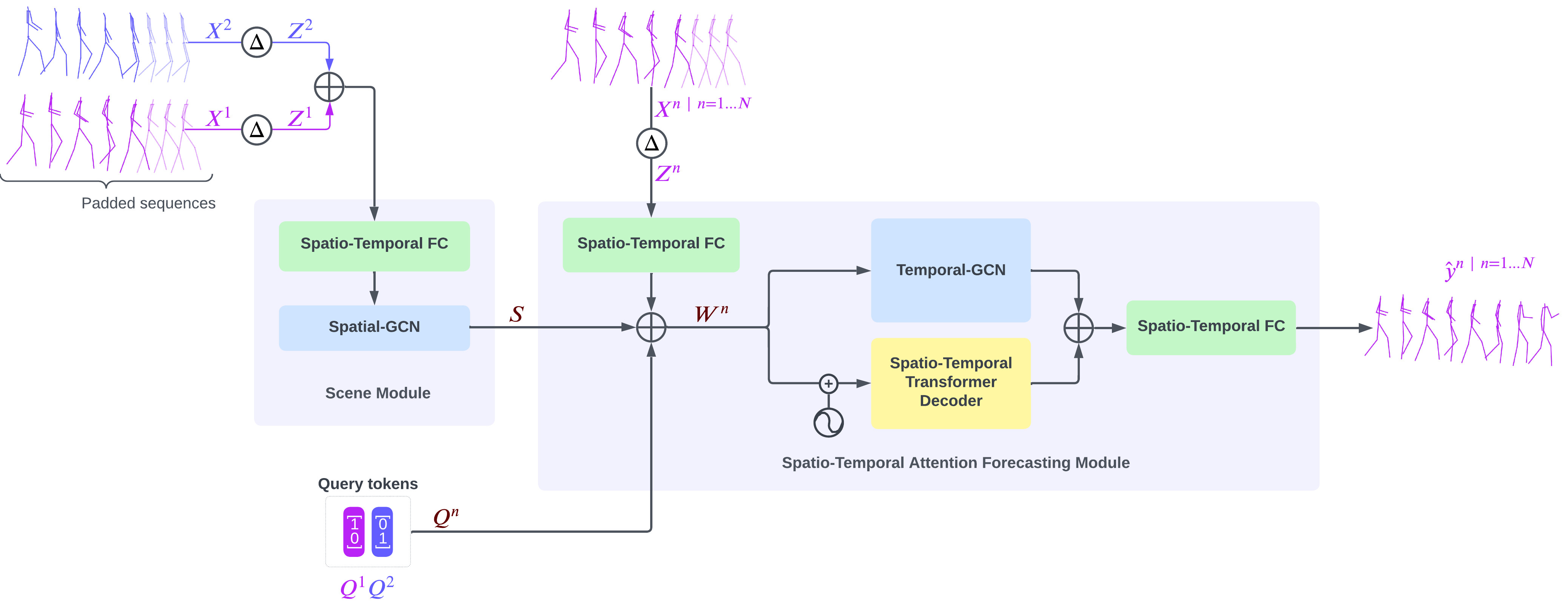
GCN-Transformer comprises two main modules: Scene Module and Spatio-Temporal Attention Forecasting Module. Initially, the input sequences are padded with the last known pose T times and augmented by incorporating their temporal differentiation, resulting in enriched sequences denoted as . These enriched sequences are concatenated and fed into the Scene Module. Within the Scene Module, a Spatio-Temporal Fully-Connected module encodes the poses into an embedding space. Subsequently, the output undergoes processing through the Spatial-GCN network designed to extract social features and dependencies. The resulting output S from the Scene Module is then forwarded into the Spatio-Temporal Attention Forecasting Module for each n-th sequence , along with a query token generated through one-hot encoding based on the position of the n-th sequence within the scene.
In the Spatio-Temporal Attention Forecasting Module, the sequence is encoded into the embedding space using a Spatio-Temporal Fully-Connected module. The resulting output is then concatenated with the extracted features S from the Scene Module and the query token to create . Subsequently, is simultaneously passed into the Spatio-Temporal Transformer Decoder and Temporal-GCN modules. The outputs from both modules are concatenated and processed through a Spatio-Temporal Fully-Connected module to generate the final prediction . The architecture of GCN-Transformer is shown in Figure 4.
5.1. Scene Module
Scene Module is designed to enhance input data representation by leveraging temporal and spatial information. It comprises two key elements: a Spatio-Temporal Fully-Connected module and the Spatial-GCN. The Spatio-Temporal Fully-Connected module serves as an initial processing unit, transforming the enriched input sequences into a higher-dimensional embedding space, refining the input data and preparing it for subsequent modules through spatial and temporal transformations. In conjunction with the Spatio-Temporal Fully-Connected module, the Spatial-GCN module serves to uncover intricate patterns embedded within the data, specifically focusing on extracting interaction dependencies and dynamics among individuals within the scene. Comprising 8 GCN blocks with learnable adjacency matrices, this module employs various techniques, including batch normalization, dropout, and Tanh activation functions, to enhance feature extraction and maintain the integrity of the structural information present in the input data. To further enhance the model’s ability to capture social dependencies and maintain realistic spatial relationships between joints of the people in the scene, we compute the inter-individual joint distance loss on the output S.
5.2. Spatio-Temporal Attention Forecasting Module
The Spatio-Temporal Attention Forecasting Module predicts future poses by synthesizing information from various sources, including the input sequence , scene context S, and positional query token associated with sequence . Initially, the input sequence undergoes encoding via the Spatio-Temporal Fully-Connected module, transforming into an embedded space. Subsequently, this encoded sequence is concatenated with the scene context S and the positional query token to form . This composite representation undergoes parallel processing through two key components: the Spatio-Temporal Transformer Decoder and the Temporal-GCN modules.
The Spatio-Temporal Transformer Decoder comprises two attention blocks positioned after the learnable positional encoding of . The first attention block is followed by fully-connected layers that operate on the spatial dimension, facilitating the extraction of spatial features. Conversely, the second attention block is followed by Temporal Convolutional Network (TCN) layers, which specialize in capturing long-term temporal dependencies and temporal patterns within the data. Concurrently, the Temporal-GCN module, composed of 8 GCN blocks with learnable adjacency matrices, operates on to extract and refine temporal dependencies, thereby enhancing the temporal representation separate from the Spatio-Temporal Transformer Decoder.
Finally, the Spatio-Temporal Attention Forecasting Module integrates the extracted features using Spatio-Temporal Fully-Connected module, resulting in the generation of final pose sequence prediction . This fusion process ensures that the module leverages the diverse information captured across spatial, temporal, and contextual dimensions to produce accurate and reliable predictions for future poses.
5.3. Data Preprocessing
We opted against employing any data preprocessing techniques for our model, instead we utilized raw data from the datasets. This approach was chosen to compel the model to learn the intricate structure of the human skeleton and the dynamic nature of movement. Conventional preprocessing methods, such as employing Discrete Cosine Transform (DCT) to encode Cartesian coordinates into frequencies, often yield poses that appear ghost-like and lack the nuanced dynamics of human movement, like in [10,12,13,14]. Moreover, techniques like predicting temporal differentiations that are subsequently added to the last known pose to generate the final result can produce invalid poses over the long term due to the model’s lack of awareness regarding human structural information, like in [9,12,15,16,17].
5.4. Data Augmentation
Data augmentation is essential for enhancing the robustness and generalization capability of pose forecasting models. Building upon methods utilized in [14], we extended the augmentation strategy with new methods to introduce further variations in the training data. Inspired by [14], we adopted several effective methods: sequence reversal, which reverses the temporal order of input sequences to expose the model to diverse temporal patterns; random person permutation, which shuffles the order of individuals within a scene to accommodate different person arrangements and interactions; random scaling, which introduces variations in pose scale to simulate varying heights of the people; random orientation, where poses are randomly rotated to simulate different camera viewpoints or human orientations; and random positioning, which shifts the positions of individuals within the scene to introduce spatial variability.
Expanding upon these methods, we introduced new techniques to enrich the dataset further. One method involved randomizing the joint order of individuals in a scene, encouraging the model to learn complex skeleton representations and adapt to different joint configurations. Additionally, we used a method to randomize the XYZ axes of individuals, enhancing pose variation by altering the orientation and positioning of poses in 3D space. Lastly, we varied the dataset sampling frequency, using frequencies 1-4 to capture slower and faster sequences, though this sampling is performed during the preprocessing step.
All augmentations, except for sampling frequencies, are applied dynamically to each sampled batch of scene sequences during training. Each augmentation method is applied with a specific probability, introducing controlled variability into the training data. For instance, sequence reversal, random person permutation, random scaling, and random positioning each have a 50% probability of being applied, while random orientation, random joint order, and random XYZ-axis order are applied with a 25% probability. Furthermore, there is a 25% probability that no augmentation will be applied to a given sequence, ensuring that the model is exposed to both augmented and unaugmented data. These augmented datasets enable the model to learn robust features and adapt effectively to diverse scenarios, improving its performance and generalization capability in pose forecasting tasks.
5.5. Training
Our model optimizes its parameters by minimizing the error between the predicted and the ground truth poses, a loss commonly referred to as reconstruction error (REC) and widely used by other models. We introduce an additional loss called Multi-person joint distance loss (MPJD) to further enhance the model representation of interpersonal interactions. This loss component encourages the Scene Module to accurately capture the interactions among individuals within the scene by penalizing the error in joint distances between individuals. By optimizing this metric, the Scene Module is encouraged to model the spatial relationships between individuals better. Additionally, we incorporate Velocity loss (VL) to promote the learning of movement dynamics. This technique prioritizes the generation of coherent pose trajectories over predicting precise poses at specific time intervals, producing more realistic and fluid motion sequences.
The final loss function is determined by combining the standard reconstruction loss with an additional Multi-person joint distance loss (MPJD), scaled by a factor denoted as , used to adjust the effect of the MPJD loss on the overall loss. Both the output and scene predictions are subjected to Velocity loss (VL), with the Velocity loss for the output from the Scene Module also scaled by the factor. To measure the error between the predicted and ground truth coordinates, we employ the -norm loss, aiming to minimize this error during training.
The final loss is calculated as follows:
where N represents the number of people in the scene, and represents predicted pose sequence of n-th and p-th person in the scene, while and represents corresponding ground truth pose sequence of n-th and p-th person in the scene. denotes the Euclidean distance (L2 norm), and represents the mean distance across all people in the scene. The represents temporal differentiation, where for and for . Predicted velocities of joint distances between individuals are represented with , while represents ground truth velocities of joint distances between individuals.
Including MPJD and VL losses in the training process significantly enhances the practical applicability of multi-person pose forecasting models in real-world scenarios. The MPJD loss encourages the model to learn interaction dynamics between individuals in a scene, helping it capture how one individual’s movements influence others. This is particularly useful in scenarios such as crowd monitoring, group behavior analysis, and human-robot collaboration, where understanding interpersonal interactions is critical. On the other hand, the VL loss emphasizes temporal velocities between subsequent poses, promoting the generation of fluid and natural motion sequences. This is crucial in applications like animation, virtual reality, and autonomous systems, where smooth and realistic motion transitions are essential. Together, these losses address the challenges of producing rigid or disconnected poses, ensuring the model generates dynamic, context-aware predictions.
We trained our model for 512 epochs with a batch size of 256 which was the largest manageable size given our hardware constraints. The extended training duration was chosen to accommodate the strong and dynamic augmentation strategy, which introduced extensive variability to the data, necessitating longer training for the model to effectively learn from these variations. Observing that the performance improvements plateaued around 512 epochs, we determined this duration was sufficient for optimal convergence. The Adam optimizer, a standard choice in pose forecasting, was chosen due to its adaptability and efficiency in handling complex, dynamic loss landscapes, especially with the strong augmentations applied. After testing multiple learning rates, we set an initial learning rate of 0.001, finding that it balanced effective learning with stability. A higher learning rate caused the loss to oscillate heavily, likely due to abrupt shifts in solution space introduced by the strong augmentation, and in some cases, gradients would explode. To guide the model closer to the optimal solution, we reduced the learning rate to 0.0001 after 256 epochs, ensuring smoother convergence in the later stages of training. We also carefully tuned the parameter, which scales the MPJD loss, by analysing values from 0 to 1. A value of 0.1 was selected, as it provided the best balance in guiding the model to capture both spatial dependencies and movement dynamics effectively.
6. Experimental Results
In our experimental evaluation of GCN-Transformer, we employed two distinct datasets: SoMoF and ExPI. To assess model performance, we define evaluation metrics that quantify the error between predicted poses and ground truth. Through comprehensive analysis, we evaluated our model’s performance on both datasets and conducted a comparative study against state-of-the-art models in the domain of multi-person pose forecasting.
6.1. Metrics
MPJPE (Mean Per Joint Position Error) is a commonly used metric for evaluating the performance of pose forecasting methods [12,13,14,15,37]. It measures the average Euclidean distance between the predicted joint positions and the corresponding ground truth positions across all joints. The lower the MPJPE value, the closer the predicted poses align with the ground truth. This metric provides a joint-level assessment of pose forecasting performance. The MPJPE metric is calculated as follows:
where f denotes a time step and denotes the corresponding skeleton. is the estimated position of joint j and is the corresponding ground truth position. represents the number of joints. denotes the Euclidean distance (L2 norm), and represents the mean distance across all joints.
Another commonly employed metric in pose forecasting evaluation is the Visibility-Ignored Metric (VIM), initially proposed by Adeli et al. in [18]. VIM is computed by assessing the mean distance between the predicted and ground truth joint positions at the last pose T. This calculation involves flattening the joint positions and coordinates dimensions into a unified vector representation, resulting in a vector dimensionality of , where J denotes the number of joints. Subsequently, the Euclidean distance (L2 norm) is computed between the corresponding ground truth and predicted joint positions. The average distance across all joints yields the final VIM score. The SoMoF Benchmark adopts this metric for its evaluation framework. The VIM metric computation can be expressed as follows:
where J represents the number of joints, is the ground-truth position of the i-th joint (flattened), is the predicted position of the i-th joint (flattened), denotes the Euclidean distance (L2 norm), and represents the mean distance across all joints.
6.2. Datasets
We employed distinct datasets for both training and evaluation, aligning with the methodology of previous models such as SoMoFormer [13], MRT [12], MPFSIR [14], and JRTransformer [15]. For training, we utilized the 3D Poses in the Wild (3DPW) [38] and Archive of Motion Capture As Surface Shapes (AMASS) [39] datasets. The 3DPW dataset contains over 60 video sequences capturing human motion in real-world scenarios, including accurate reference 3D poses in natural scenes such as people shopping in the city, having coffee, or doing sports, recorded with a moving hand-held camera. To adhere to the evaluation protocol of the SoMoF benchmark [18], we employed a specific split of the 3DPW dataset, where the train and test sets are inverted. Thus, we trained all models on the 3DPW test set and subsequently evaluated them on the 3DPW train set. This inversion was originally introduced by the authors of the SoMoF benchmark [18] due to the preprocessing of the 3DPW dataset, which created a larger number of sequences in the test set than in the training set, thus inverting the datasets allowed for a more robust training set. By following this protocol, we ensure that our results are directly comparable with other multi-person pose forecasting models evaluated under the same conditions. Specifically, for the SoMoF test set, data from the original 3DPW training set was sampled without overlap, producing distinct pose sequences. In contrast, the SoMoF training set was generated by sampling the original 3DPW testing set with overlap, employing a sliding window of 1 to capture a broader range of pose variations. The validation set remained consistent with the original 3DPW dataset, sampled without overlap.
On the other hand, the AMASS dataset provides an extensive collection of human motion capture sequences, totaling over 40 hours of motion data and 11,000 motions represented as SMPL mesh models. During the training process, we utilized the CMU, BMLMovi, and BMLRub subsets of the AMASS dataset, which provided a diverse and large-scale dataset. Given that many sequences within this dataset are single-person, we employed a technique to synthesize additional training data by combining sampled sequences to generate multi-person training data.
In contrast to recent works [12,13,14,15,16] utilizing datasets like Carnegie Mellon University Motion Capture Database (CMU-Mocap) [40] and Multi-person Pose estimation Test Set in 3D (MuPoTS-3D) [41] alongside the SoMoF Benchmark for model evaluation, our study opts not to include these datasets. The decision stems from the observation that CMU-Mocap and MuPoTS-3D datasets primarily feature simplistic movements and minimal interactions, often resulting in sequences where individuals maintain the same pose and position. Consequently, models trained on these datasets tend to predict repetitive or static poses, failing to showcase their true potential in pose forecasting. Instead, we use the Extreme Pose Interaction (ExPI) [42] dataset that contains dynamic sequences involving two couples engaged in various actions with significant movement providing a more challenging and realistic evaluation environment.
6.3. Results on SoMoF Benchmark
The SoMoF benchmark, introduced by Adeli et al. in [18], serves as a standardized assessment platform for evaluating the performance of multi-person pose forecasting models. The SoMoF benchmark is derived from the 3DPW dataset, where every other frame is sampled to lower the original frames per second (FPS) from 30 to 15. This benchmark task involves predicting the subsequent 14 frames (equivalent to 930 milliseconds) based on 16 frames (1070 milliseconds) of preceding input data, encompassing joint positions for multiple individuals. The evaluation uses the Visibility-Ignored Metric (VIM), measuring performance across various future time steps. Similarly to [10,13,14,15], all evaluated models in this paper were trained to utilize data from the 3DPW [38] and AMASS [39] datasets. During training, emphasis was placed solely on the 13 joints evaluated within the SoMoF framework. To ensure fairness in comparison, a practice observed in various studies such as [15,16,17] was adopted, whereby the final results are reported based on the epoch with the lowest average VIM score on the test dataset. Furthermore, problem formulation remained consistent for all evaluated models, focusing on predicting the next 14 frames using 16 input data frames. This differs from methodologies advocated by [10,13,15] to divide formulation into two separate problem formulations for short-term and long-term optimization, which inherently enhances model performance.
We conducted a comparative analysis of evaluated methods on the SoMoF Benchmark test set, as presented in Table 1, demonstrating that our model consistently achieves state-of-the-art results compared to competing models.
The results demonstrate the superior performance of GCN-Transformer across both VIM and MPJPE metrics, establishing it as a state-of-the-art solution in multi-person pose forecasting. While SoMoFormer emerges as a formidable competitor, particularly in long-term forecasting, GCN-Transformer consistently outperforms all models, especially when considering the overall metric, which aggregates performance across all evaluated time intervals. Interestingly, despite the reported similar performance to SoMoFormer, JRTransformer fails to achieve competitive results in this evaluation. Conversely, the Future Motion model, introduced in 2021, demonstrates commendable performance, rivaling even the most recent state-of-the-art models. The MPFSIR model is not far off either, achieving this performance with only a fraction of parameters compared to others. Finally, GCN-Transformer* showcases significantly superior results, owing to its training with an integrated validation dataset. This variant currently leads the official SoMoF Benchmark leaderboard at https://somof.stanford.edu.
Figure 5 shows the predicted poses for two sequences from the SoMoF Benchmark test set, comparing the performance of the best-performing models: JRTransformer, SoMoFormer, and GCN-Transformer, with the ground truth (GT) also displayed for comparison. The figures reveal that both JRTransformer and SoMoFormer encounter difficulties in generating valid poses, often producing unrealistic joint configurations and movements. In contrast, the GCN-Transformer model demonstrates a clear advantage, consistently generating valid poses and realistic movements.
6.4. Results on ExPI dataset
The Extreme Pose Interaction (ExPI) dataset, described in [42], features two couples of dancers engaging in 16 distinct extreme actions. These actions include aerial maneuvers, with the first seven being performed by both dancer couples. Subsequently, six additional aerials are executed by Couple 1, while the remaining three are carried out by Couple 2. Each action is repeated five times to capture variability, resulting in a collection of 115 sequences recorded at 25 frames per second (FPS) and 60,000 annotated 3D body poses.
Taking inspiration from the data partitioning outlined in [42], we designate all actions executed by Couple 2 as the training set and those performed by Couple 1 as the test set. This approach deviates slightly from the dataset division presented by Guo et al. in [42], as we incorporate common actions performed by both couples and actions performed exclusively by one couple into the training set. This dataset split emulates both the Common action split and Unseen action split described in [42], consolidating them into a single split.
We employ a sliding-window technique with overlapping sequences to sample the training data, whereas the testing data is sampled sequentially without overlaps. Additionally, we downsample each sequence by selecting every other frame, reducing the original frames per second (FPS) from 25 to 12.5 FPS. Following the precedent set by the SoMoF Benchmark, we utilize 16 frames (equivalent to 1280 milliseconds) to predict the subsequent 14 frames (equivalent to 1080 milliseconds). Moreover, we apply a scaling factor of 0.39 to maintain consistency in person scale with the SoMoF Benchmark, the dataset on which the models are developed.
We conducted a comparative analysis of evaluated methods on the ExPI test set, as presented in Table 2, demonstrating that our model consistently achieves state-of-the-art results compared to competing models. The results on the ExPI dataset differ significantly from those on the SoMoF Benchmark dataset, revealing notable performance degradations in some of the previously strong models. SoMoFormer, a close competitor on the SoMoF Benchmark, performs substantially worse on the ExPI dataset, surpassed by JRTransformer and MPFSIR. This drop in performance highlights the model’s sensitivity to different dataset characteristics. Similarly, the Future Motion model, which had proven to be a strong contender on the SoMoF Benchmark, is now outperformed by almost all other models. This indicates that the Future Motion model’s performance is heavily influenced by the dataset characteristics, showcasing its lack of robustness across diverse data scenarios. Interestingly, JRTransformer, which was not as competitive on the SoMoF Benchmark, emerges as a close competitor to GCN-Transformer on the ExPI dataset. Despite this, GCN-Transformer remains the clear winner across all time intervals, reaffirming its superior performance and generalizability.
Figure 6 shows the predicted poses for two sequences from the ExPI test set, showcasing the performance of the best-performing models: JRTransformer, SoMoFormer, and GCN-Transformer, with the ground truth (GT) also displayed for comparison. The results highlight a significant distinction in model performance. JRTransformer and SoMoFormer struggle to generate valid movements, often defaulting to repeating the last known pose rather than predicting dynamic and realistic trajectories. In contrast, the GCN-Transformer model maintains the integrity of the poses and successfully predicts realistic and coherent movement patterns.
7. Ablation Study
We conducted an ablation study on GCN-Transformer to systematically assess the impact of different components and methods on the model’s performance. This comprehensive analysis involved iteratively integrating various components and methods into the baseline model and evaluating performance at each stage. Initially, we established a baseline model comprising a Scene Module and Spatio-Temporal Transformer Decoder. Subsequently, we extend the Spatio-Temporal Attention Forecasting Module with Temporal-GCN, slightly enhancing model performance. Next, we introduced Multi-person joint distance (MPJD) loss, further improving both short-term and long-term forecasting accuracy. Incorporating Velocity loss yielded a marginal improvement in overall performance, enhancing intra-sequence accuracy while slightly compromising short-term accuracy. Lastly, adding data augmentation significantly improved the model performance across all evaluated time intervals, representing the most substantial improvement among all modifications. Table 3 presents the evaluation results of each model on VIM and MPJPE metrics, trained exclusively on the 3DPW training set and tested on the SoMoF Benchmark validation set.
8. FJPTE: FINAL JOINT POSITION AND TRAJECTORY ERROR
The evaluation of pose forecasting models involves adopting and adapting various metrics borrowed from related tasks, such as pose estimation [43,44]. Initially, the Mean Per Joint Position Error (MPJPE) metric, borrowed from pose estimation, was widely used. However, it calculates the Euclidean distance (L2 norm) across all joints in the predicted sequence, providing an overall assessment of model performance without specifically focusing on human movement dynamics.
To address this limitation, Adeli et al. in [18] introduced the Visibility-Ignored Metric (VIM). Unlike MPJPE, VIM evaluates the pose error solely at the last predicted frame, overlooking the trajectory of joints in preceding frames and focusing solely on the final pose error.
Building upon the MPJPE metric, Šajina and Ivasic-Kos in [14] proposed the Movement-Weighted Mean Per Joint Position Error (MW-MPJPE). This metric enhances MPJPE by incorporating a weighting factor based on the overall movement exhibited by the individual throughout the target pose sequence. This weighting factor provides a more nuanced evaluation by considering the varying degrees of movement across different poses.
Peng et al. in [16] employed various evaluation metrics to assess multi-person pose forecasting models. These included Joint Position Error (JPE), which resembles MPJPE but reports errors for all individuals in the scene, Aligned Mean Per Joint Position Error (APE), akin to Root-MPJPE, focusing on pose position error by removing global movement, and Final Displacement Error (FDE), measuring trajectory prediction error by considering only the final global position (e.g., pelvis) of each person.
The multitude of metrics available for pose forecasting complicates the evaluation process, as different metrics assess distinct aspects of model performance. Consequently, model rankings can vary significantly depending on the chosen evaluation metric, making it challenging to identify the optimal model for the task. To address this issue, we introduce a novel metric,
Final Joint Position and Trajectory Error (FJPTE), designed to consolidate the diverse objectives of pose forecasting into a single comprehensive measure. Our metric aims to capture key goals of pose forecasting, including predicting the final (N-th frame) global position (e.g., pelvis) and the trajectory of global movement leading up to that position, as well as forecasting the final pose position without global movement and its accompanying trajectory. FJPTE tackles this challenge by independently evaluating four distinct components and aggregating their results: the error in the final global position (measured by Euclidean distance), the error of global movement trajectory (measured using Euclidean distance of temporal differentiation of root joint), the error in the final pose position excluding global movement (assessed using Euclidean distance), and the trajectory error of pose position without global movement (measured using Euclidean distance of temporal differentiation for all pose joints). Through this comprehensive approach, FJPTE provides a holistic assessment of a model’s performance, capturing its proficiency in capturing natural human motion dynamics and the validity of its predicted poses. An illustrative comparison of joint movement evaluation using our metric is presented in Figure 7.
Additionally, Figure 8 illustrates an example where FJPTE provides a more comprehensive evaluation than MPJPE or VIM. The example shows a predicted sequence where the global position is accurate, but the pose remains frozen or ghost-like, floating unnaturally through global space, an issue commonly seen in pose forecasting. Unlike MPJPE, which evaluates joint distances independently across time intervals, or VIM, which focuses solely on the final interval (), FJPTE comprises two key components: movement dynamics (FJPTElocal) and global position and trajectory (FJPTEglobal). By breaking down errors into these components, FJPTE identifies whether a model struggles more with local movement dynamics or global trajectory alignment. Furthermore, by combining these errors, FJPTE enables a holistic evaluation and effective ranking of models based on their overall performance.
FJPTE is calculated as follows:
where denotes the predicted sequence, while y denotes the ground truth sequence. The number of joints is denoted with J, while the number of time intervals is denoted with T. denotes the Euclidean distance (L2 norm), and represents the mean errors across all time intervals. represents global position and trajectory error between predicted and ground truth sequence, measured at the pelvis joint. represents local movement dynamic error between predicted and ground truth sequence excluding the pelvis joint and global movement. unifies local and global error into a single metric.
We compared evaluated models using the proposed FJPTElocal and FJPTEglobal metrics on the SoMoF Benchmark test set and reported results in Table 4. Results demonstrate that GCN-Transformer significantly outperforms all other models on the FJPTElocal metric. This underscores GCN-Transformer’s superior ability to model human movement dynamics and interaction dynamics compared to other models. While the overall performance hierarchy of the models remains consistent with evaluations using VIM and MPJPE metrics, LTD and JRTransformer exhibit slightly better performance in modeling movement dynamics than their immediate competitors, TBIFormer and MPFSIR. When assessing the FJPTEglobal metric, GCN-Transformer shows a slight performance gap behind SoMoFormer in long-term forecasting, indicating that SoMoFormer has a marginal edge in predicting long-term global movements. Additionally, MPFSIR emerges as a notable performer, significantly outperforming its closest competitor, Future Motion, in forecasting global positions and trajectories.
Similarly, Table 5 presents the performance of evaluated models on the ExPI test set using the proposed FJPTElocal and FJPTEglobal metrics. The results indicate that GCN-Transformer consistently outperforms all other models on the FJPTElocal metric, except at the 120ms time interval, where JRTransformer marginally surpasses GCN-Transformer. Notably, SoMoFormer confirms it is struggling with this dataset, while JRTransformer confirms it to be a strong contender. Another key observation is that LTD outperformed MRT on this metric, compared to evaluations using VIM and MPJPE metrics. When examining the FJPTEglobal metric, GCN-Transformer narrowly outperforms JRTransformer, demonstrating a slight edge in overall performance despite JRTransformer’s better short-term forecasting capabilities. SoMoFormer again shows a notable decline in performance, finishing behind both JRTransformer and MPFSIR. The overall performance hierarchy of the models on the ExPI dataset remains consistent with their evaluations using VIM and MPJPE metrics.
These results indicate that models can perform well on VIM and MPJPE metrics by focusing on global movement or movement dynamics, as models typically excel in one of these areas but not both. In contrast, FJPTElocal and FJPTEglobal provide a clear distinction, making it easier to identify the best-performing models for each specific area.
Table 6 presents a comprehensive evaluation of forecasting errors using the proposed FJPTE metric, which combines FJPTElocal and FJPTEglobal. On the SoMoF Benchmark test set, SoMoFormer emerges as the leading model, with only GCN-Transformer*, which included the validation set during training, surpassing its performance. Most models maintain a similar performance hierarchy as seen with VIM and MPJPE evaluations, although LTD notably outperforms both TBIFormer and MRT.
In contrast, the ExPI test set results highlight GCN-Transformer as the top performer overall. While JRTransformer slightly outperforms GCN-Transformer in short-term forecasting, GCN-Transformer consistently delivers superior results across broader time intervals. The performance ranking of other models remains largely consistent with the VIM and MPJPE evaluations. However, LTD surpasses MRT, and DViTA outperforms Future Motion, making Future Motion the lowest-performing model on the ExPI dataset using FJPTE.
To summarize, the proposed FJPTE metric significantly enhances the evaluation of pose forecasting models by providing a more detailed analysis of movement dynamics alongside global position and trajectory errors. FJPTE delivers valuable insights into how accurately predictions capture realistic motion, as demonstrated in Figure 7 and Figure 8. These examples highlight the metric’s ability to pinpoint errors in movement dynamics versus global position and trajectory deviations, offering greater clarity during evaluation. This precision is particularly impactful in applications such as surveillance, animation, and autonomous systems, where natural movement dynamics are essential for effective human-robot interaction, motion tracking, and scene understanding. By quantifying both global alignment and detailed movement nuances, FJPTE ensures models are rewarded for producing smooth, realistic motion. Furthermore, its focus on dynamics helps mitigate common issues such as ghost-like poses or unrealistic trajectories, boosting the robustness of models in real-world, dynamic scenarios.
9. Limitations
While GCN-Transformer demonstrates state-of-the-art performance in multi-person pose forecasting, it is not without its limitations. A key drawback of the model lies in its size; GCN-Transformer has a large number of parameters (~5.9M), which makes it computationally expensive and memory-intensive compared to lighter models like MPFSIR (~0.15M). While MPFSIR performs nearly as well as state-of-the-art models with significantly fewer parameters, GCN-Transformer’s parameter count is more comparable to its closest competitors, SoMoFormer (~4.9M) and JRTransformer (~3.6M), which mitigates this limitation to some extent. However, this still poses challenges for deployment in resource-constrained environments.
A more critical limitation, shared by GCN-Transformer and other models in the field, is the inability to forecast movements that are not represented in the training dataset. When encountering novel movements, models tend to repeat the last observed poses, resulting in frozen or static sequences. Figure 9 illustrates examples from the SoMoF and ExPI datasets, where unseen movements lead to poor forecasts. In such cases, the model fails to generalize effectively, underscoring the importance of diverse and representative training datasets to address this issue.
Another limitation of GCN-Transformer is the complexity of training due to its reliance on strong augmentations. While these augmentations improve generalization, they also necessitate longer training cycles and careful hyperparameter tuning to stabilize learning. Furthermore, despite its ability to capture interactions and dependencies between individuals, the model may struggle in scenes with highly intricate or unusual social dynamics, where interactions are more ambiguous or rare.
Lastly, the evaluation of model performance still heavily relies on benchmark datasets, which may not fully capture the diversity and variability of real-world scenarios. Consequently, there remains room for improvement in assessing and optimizing model robustness for broader applications.
These limitations provide avenues for future research, including developing lighter models with comparable performance, improving generalization to unseen movements, and enhancing training and evaluation protocols to better reflect real-world complexities.
10. Conclusion
In conclusion, this paper introduces GCN-Transformer, a novel model for multi-person pose forecasting that leverages the synergies of Graph Convolutional Network and Transformer architectures. We conducted a thorough evaluation of GCN-Transformer alongside other state-of-the-art models, presenting results on the SoMoF Benchmark and ExPI datasets using the VIM and MPJPE metrics. The results on the SoMoF Benchmark should be cautiously interpreted due to the dataset’s inherent randomness, attributed to sequences recorded with a moving camera. This introduces complexities as models must predict human and camera movements, often perceived as erratic. To mitigate this, we additionally evaluated all models on the ExPI dataset, featuring challenging actions performed by two couples without camera movement. Conclusively, GCN-Transformer consistently outperforms existing state-of-the-art models on both datasets.
Furthermore, we propose a novel evaluation metric, FJPTE, which comprehensively assesses pose forecasting error by accounting for both local movement dynamics (FJPTElocal) and global movement (FJPTEglobal). These components are computed based on errors at the final position and along the trajectory leading up to that point. Our evaluation of all models using FJPTE reveals that GCN-Transformer excels in capturing both intricate movement dynamics and accurate global position trajectory, where it consistently achieves state-of-the-art results.
Overall, the success of GCN-Transformer underscores its potential to drive the field of multi-person pose forecasting, with promising applications in human-computer interaction, sports analysis, and augmented reality. As future work, we aim to explore further enhancements to GCN-Transformer architecture, including the integration of activity recognition to aid with pose forecasting and investigate its applicability to real-world scenarios.
Author Contributions
Conceptualization, R.Š., G.O. and M.I-K.; methodology, R.Š.; software, R.Š. and G.O.; validation, R.Š., G.O. and M.I-K.; formal analysis, R.Š.; investigation, R.Š. and G.O.; resources, R.Š.; data curation, R.Š.; writing—original draft preparation, R.Š.; writing—review and editing, R.Š., G.O. and M.I-K.; visualization, R.Š.; supervision, M.I-K; project administration, M.I-K.; funding acquisition, M.I-K. All authors have read and agreed to the published version of the manuscript.
Funding
This research was funded by Croatian Science Foundation under the project IP-2016-06-8345, "Automatic recognition of actions and activities in multimedia content from the sports domain" (RAASS), and by the University of Rijeka (project number uniri-iskusni-drustv-23-278).
Institutional Review Board Statement
Not applicable.
Informed Consent Statement
Not applicable.
Data Availability Statement
The original data presented in the study are openly available in https://github.com/RomeoSajina/GCN-Transformer.
Conflicts of Interest
The authors declare no conflicts of interest.
References
- Chiu, H.k.; Adeli, E.; Wang, B.; Huang, D.A.; Niebles, J.C. Action-agnostic human pose forecasting. In Proceedings of the 2019 IEEE winter conference on applications of computer vision (WACV). IEEE; 2019; pp. 1423–1432. [Google Scholar]
- Huang, Y.; Bi, H.; Li, Z.; Mao, T.; Wang, Z. Stgat: Modeling spatial-temporal interactions for human trajectory prediction. In Proceedings of the Proceedings of the IEEE/CVF international conference on computer vision; 2019, pp. 6272–6281.
- Mao, W.; Liu, M.; Salzmann, M.; Li, H. Learning trajectory dependencies for human motion prediction. In Proceedings of the Proceedings of the IEEE/CVF International Conference on Computer Vision; 2019, pp. 9489–9497.
- Medjaouri, O.; Desai, K. Hr-stan: High-resolution spatio-temporal attention network for 3d human motion prediction. In Proceedings of the Proceedings of the IEEE/CVF Conference on Computer Vision and Pattern Recognition; 2022, pp. 2540–2549.
- He, X.; Zhang, W.; Li, X.; Zhang, X. TEA-GCN: Transformer-Enhanced Adaptive Graph Convolutional Network for Traffic Flow Forecasting. Sensors 2024, 24. [Google Scholar] [CrossRef] [PubMed]
- Jiang, J.; Yan, K.; Xia, X.; Yang, B. A Survey of Deep Learning-Based Pedestrian Trajectory Prediction: Challenges and Solutions. Sensors 2025, 25. [Google Scholar] [CrossRef] [PubMed]
- Guo, W.; Du, Y.; Shen, X.; Lepetit, V.; Alameda-Pineda, X.; Moreno-Noguer, F. Back to mlp: A simple baseline for human motion prediction. In Proceedings of the Proceedings of the IEEE/CVF Winter Conference on Applications of Computer Vision; 2023, pp. 4809–4819.
- Bouazizi, A.; Holzbock, A.; Kressel, U.; Dietmayer, K.; Belagiannis, V. MotionMixer: MLP-based 3D Human Body Pose Forecasting. In Proceedings of the Proceedings of the Thirty-First International Joint Conference on Artificial Intelligence, IJCAI-22; Raedt, L.D., Ed. International Joint Conferences on Artificial Intelligence Organization, 7 2022, pp. 791–798. Main Track.
- Parsaeifard, B.; Saadatnejad, S.; Liu, Y.; Mordan, T.; Alahi, A. Learning decoupled representations for human pose forecasting. In Proceedings of the Proceedings of the IEEE/CVF International Conference on Computer Vision, 2021, pp. 2294–2303.
- Wang, C.; Wang, Y.; Huang, Z.; Chen, Z. Simple baseline for single human motion forecasting. In Proceedings of the Proceedings of the IEEE/CVF International Conference on Computer Vision, 2021, pp. 2260–2265.
- Jaramillo, I.E.; Chola, C.; Jeong, J.G.; Oh, J.H.; Jung, H.; Lee, J.H.; Lee, W.H.; Kim, T.S. Human Activity Prediction Based on Forecasted IMU Activity Signals by Sequence-to-Sequence Deep Neural Networks. Sensors 2023, 23. [Google Scholar] [CrossRef] [PubMed]
- Wang, J.; Xu, H.; Narasimhan, M.; Wang, X. Multi-person 3D motion prediction with multi-range transformers. Advances in Neural Information Processing Systems 2021, 34, 6036–6049. [Google Scholar]
- Vendrow, E.; Kumar, S.; Adeli, E.; Rezatofighi, H. SoMoFormer: Multi-Person Pose Forecasting with Transformers. arXiv 2022, arXiv:2208.14023 2022. [Google Scholar]
- Šajina, R.; Ivasic-Kos, M. MPFSIR: An Effective Multi-Person Pose Forecasting Model With Social Interaction Recognition. IEEE Access 2023, 11, 84822–84833. [Google Scholar] [CrossRef]
- Xu, Q.; Mao, W.; Gong, J.; Xu, C.; Chen, S.; Xie, W.; Zhang, Y.; Wang, Y. Joint-Relation Transformer for Multi-Person Motion Prediction. In Proceedings of the Proceedings of the IEEE/CVF International Conference on Computer Vision, 2023, pp. 9816–9826.
- Peng, X.; Mao, S.; Wu, Z. Trajectory-aware body interaction transformer for multi-person pose forecasting. In Proceedings of the Proceedings of the IEEE/CVF Conference on Computer Vision and Pattern Recognition, 2023, pp. 17121–17130.
- Peng, X.; Zhou, X.; Luo, Y.; Wen, H.; Ding, Y.; Wu, Z. The MI-Motion Dataset and Benchmark for 3D Multi-Person Motion Prediction. arXiv 2023, arXiv:2306.13566 2023. [Google Scholar]
- Adeli, V.; Ehsanpour, M.; Reid, I.; Niebles, J.C.; Savarese, S.; Adeli, E.; Rezatofighi, H. Tripod: Human trajectory and pose dynamics forecasting in the wild. In Proceedings of the Proceedings of the IEEE/CVF International Conference on Computer Vision, 2021, pp. 13390–13400.
- Mao, W.; Hartley, R.I.; Salzmann, M.; et al. Contact-aware human motion forecasting. Advances in Neural Information Processing Systems 2022, 35, 7356–7367. [Google Scholar]
- Zhong, C.; Hu, L.; Zhang, Z.; Ye, Y.; Xia, S. Spatio-temporal gating-adjacency gcn for human motion prediction. In Proceedings of the Proceedings of the IEEE/CVF Conference on Computer Vision and Pattern Recognition, 2022, pp. 6447–6456.
- Jeong, J.; Park, D.; Yoon, K.J. Multi-agent Long-term 3D Human Pose Forecasting via Interaction-aware Trajectory Conditioning. In Proceedings of the Proceedings of the IEEE/CVF Conference on Computer Vision and Pattern Recognition, 2024, pp. 1617–1628.
- Tanke, J.; Zhang, L.; Zhao, A.; Tang, C.; Cai, Y.; Wang, L.; Wu, P.C.; Gall, J.; Keskin, C. Social diffusion: Long-term multiple human motion anticipation. In Proceedings of the Proceedings of the IEEE/CVF International Conference on Computer Vision, 2023, pp. 9601–9611.
- Xu, S.; Wang, Y.X.; Gui, L. Stochastic multi-person 3d motion forecasting. In Proceedings of the The Eleventh International Conference on Learning Representations, 2023.
- Li, L.; Pagnucco, M.; Song, Y. Graph-based spatial transformer with memory replay for multi-future pedestrian trajectory prediction. In Proceedings of the Proceedings of the IEEE/CVF conference on computer vision and pattern recognition, 2022, pp. 2231–2241.
- Aydemir, G.; Akan, A.K.; Güney, F. Adapt: Efficient multi-agent trajectory prediction with adaptation. In Proceedings of the Proceedings of the IEEE/CVF International Conference on Computer Vision, 2023, pp. 8295–8305.
- Hu, X.; Zhang, Z.; Fan, Z.; Yang, J.; Yang, J.; Li, S.; He, X. GCN-Transformer-Based Spatio-Temporal Load Forecasting for EV Battery Swapping Stations under Differential Couplings. Electronics 2024, 13, 3401. [Google Scholar] [CrossRef]
- Xiong, L.; Su, L.; Wang, X.; Pan, C. Dynamic adaptive graph convolutional transformer with broad learning system for multi-dimensional chaotic time series prediction. Applied Soft Computing 2024, 157, 111516. [Google Scholar] [CrossRef]
- Zhai, K.; Nie, Q.; Ouyang, B.; Li, X.; Yang, S. Hopfir: Hop-wise graphformer with intragroup joint refinement for 3d human pose estimation. In Proceedings of the Proceedings of the IEEE/CVF International Conference on Computer Vision, 2023, pp. 14985–14995.
- Cheng, H.; Wang, J.; Zhao, A.; Zhong, Y.; Li, J.; Dong, L. Joint graph convolution networks and transformer for human pose estimation in sports technique analysis. Journal of King Saud University - Computer and Information Sciences 2023, 35, 101819. [Google Scholar] [CrossRef]
- Bruna, J.; Zaremba, W.; Szlam, A.; LeCun, Y. Spectral networks and locally connected networks on graphs. arXiv 2013, arXiv:1312.6203 2013. [Google Scholar]
- Atwood, J.; Towsley, D. Diffusion-convolutional neural networks. Advances in neural information processing systems 2016, 29. [Google Scholar]
- Kipf, T.N.; Welling, M. Semi-supervised classification with graph convolutional networks. arXiv 2016, arXiv:1609.02907 2016. [Google Scholar]
- Cui, Q.; Sun, H.; Yang, F. Learning dynamic relationships for 3d human motion prediction. In Proceedings of the Proceedings of the IEEE/CVF conference on computer vision and pattern recognition, 2020, pp. 6519–6527.
- Vaswani, A. Attention is all you need. Advances in Neural Information Processing Systems 2017.
- Mart’inez-Gonz’alez, A.; Villamizar, M.; Odobez, J.M. Pose transformers (potr): Human motion prediction with non-autoregressive transformers. In Proceedings of the Proceedings of the IEEE/CVF International Conference on Computer Vision, 2021, pp. 2276–2284.
- Peng, X.; Shen, Y.; Wang, H.; Nie, B.; Wang, Y.; Wu, Z. SoMoFormer: Social-Aware Motion Transformer for Multi-Person Motion Prediction. arXiv 2022, arXiv:2208.09224 2022. [Google Scholar]
- Mao, W.; Liu, M.; Salzmann, M. History repeats itself: Human motion prediction via motion attention. In Proceedings of the Computer Vision–ECCV 2020: 16th European Conference, Glasgow, UK, August 23–28, 2020, Proceedings, Part XIV 16. Springer, 2020, pp. 474–489.
- Von Marcard, T.; Henschel, R.; Black, M.J.; Rosenhahn, B.; Pons-Moll, G. Recovering accurate 3d human pose in the wild using imus and a moving camera. In Proceedings of the Proceedings of the European conference on computer vision (ECCV), 2018, pp. 601–617.
- Mahmood, N.; Ghorbani, N.; Troje, N.F.; Pons-Moll, G.; Black, M.J. AMASS: Archive of motion capture as surface shapes. In Proceedings of the Proceedings of the IEEE/CVF international conference on computer vision, 2019, pp. 5442–5451.
- Carnegie Mellon University Motion Capture Database.
- Mehta, D.; Sotnychenko, O.; Mueller, F.; Xu, W.; Sridhar, S.; Pons-Moll, G.; Theobalt, C. Single-shot multi-person 3d pose estimation from monocular rgb. In Proceedings of the 2018 International Conference on 3D Vision (3DV). IEEE, 2018, pp. 120–130.
- Guo, W.; Bie, X.; Alameda-Pineda, X.; Moreno-Noguer, F. Multi-person extreme motion prediction. In Proceedings of the Proceedings of the IEEE/CVF Conference on Computer Vision and Pattern Recognition, 2022, pp. 13053–13064.
- Šajina, R.; Ivašić-Kos, M. 3D Pose Estimation and Tracking in Handball Actions Using a Monocular Camera. Journal of Imaging 2022, 8, 308. [Google Scholar] [CrossRef] [PubMed]
- Lie, W.N.; Vann, V. Estimating a 3D Human Skeleton from a Single RGB Image by Fusing Predicted Depths from Multiple Virtual Viewpoints. Sensors 2024, 24. [Google Scholar] [CrossRef] [PubMed]
Figure 1.
The figure depicts a multi-layer Graph Convolutional Network (GCN) architecture. The graph structure, defined by the normalized adjacency matrix , is shared across all layers (edges shown as black lines). The input data (with C channels) is iteratively transformed at each layer l using and a learnable weight matrix . The final layer outputs feature maps F, capturing node relationships and properties through stacked graph convolutions.
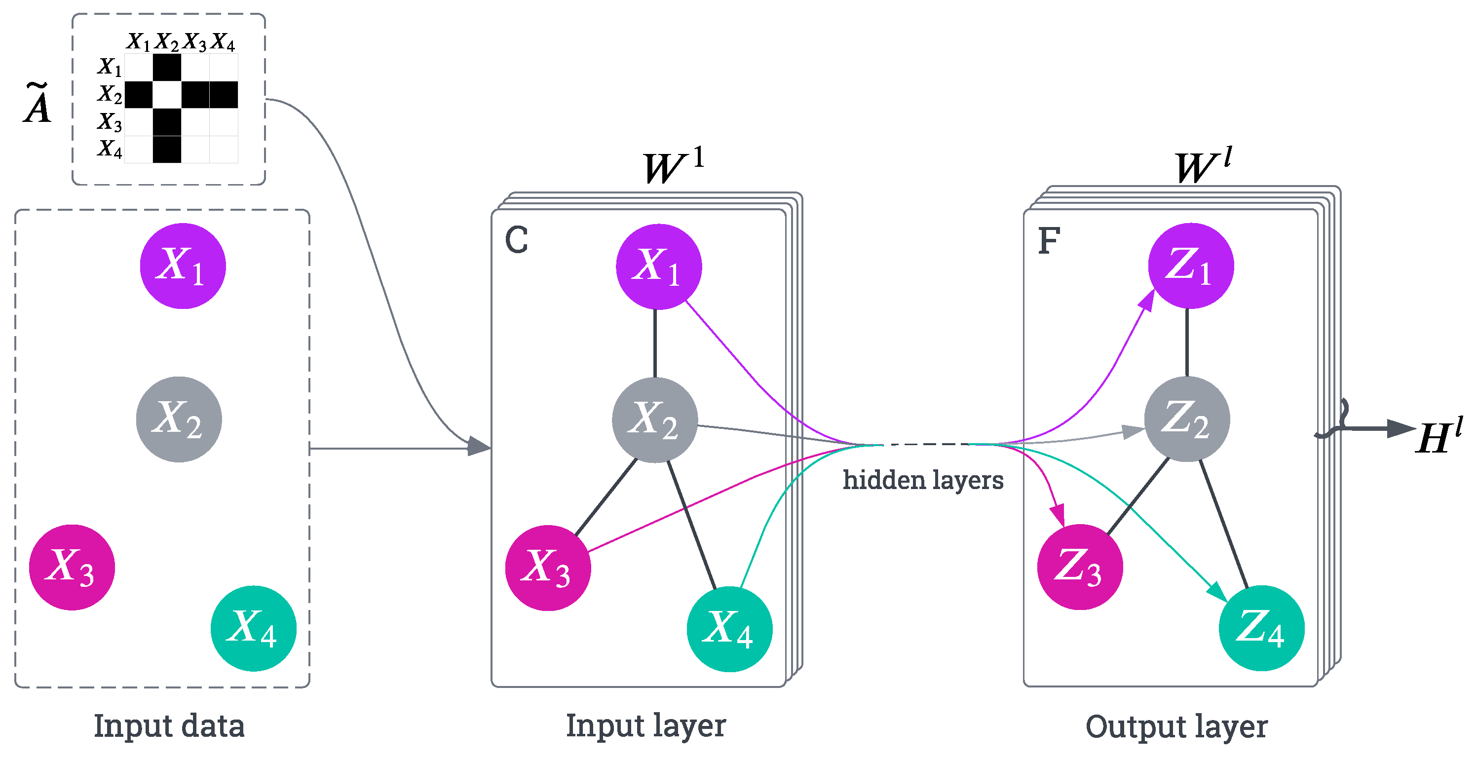
Figure 2.
The figure illustrates the attention mechanism used in Transformer architecture. The left side depicts Scaled Dot-Product Attention, where the attention scores are computed using queries (Q), keys (K), and values (V), followed by scaling and a softmax operation. The right side shows Multi-Head Attention, consisting of multiple parallel Scaled Dot-Product Attention layers. The outputs of these parallel layers are concatenated and linearly transformed to produce the final attention output.
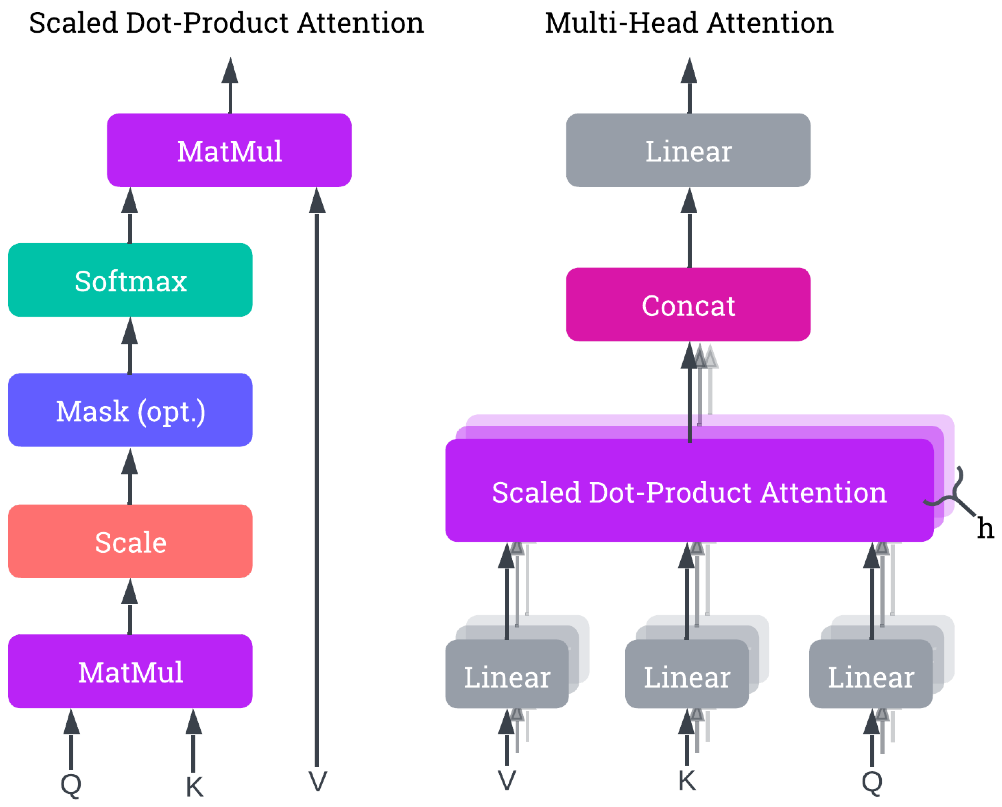
Figure 3.
The figure illustrates the problem formulation for predicting the future movements of multiple individuals in a scene. Each individual is represented by joints (e.g., elbows, knees, shoulders), and the task is to forecast their trajectories over T timesteps. The model receives historical pose sequences for each individual n, containing the positional data of joints in three-dimensional Cartesian coordinates. The objective is to predict future pose sequences , extending T timesteps into the future.
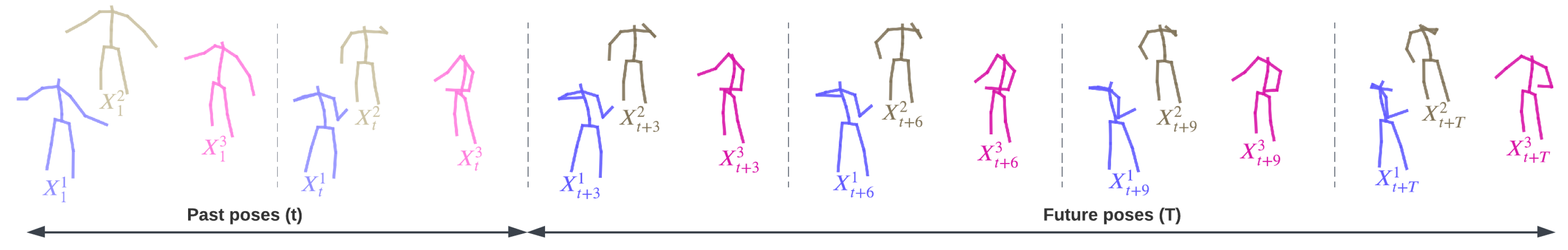
Figure 4.
The figure depicts the architecture of the GCN-Transformer model. In the preprocessing step, the input sequences and are padded with the last pose to match the full length of the sequence and are enriched with their temporal differentiation , resulting in sequences and . These sequences are then jointly processed by the Scene Module to extract social features and dependencies, producing the output S. Finally, to produce the final predictions, the output S is subsequently fed into the Spatio-Temporal Attention Forecasting Module for each n-th sequence , along with a query token generated via one-hot encoding based on the position of the n-th sequence within the scene.
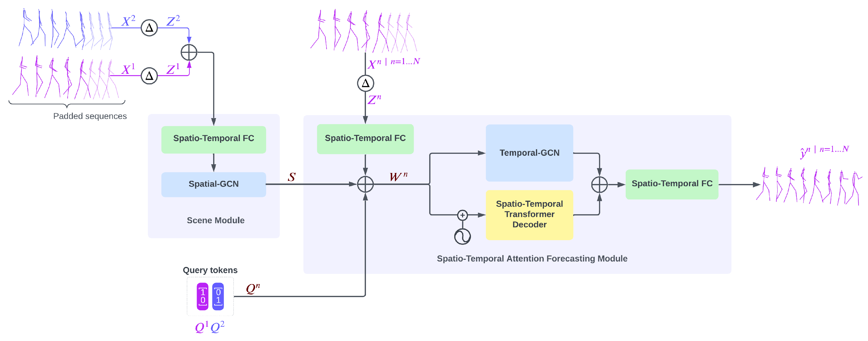
Figure 5.
The figure displays predicted poses on two example sequences from the SoMoF Benchmark test set for the best-performing models: JRTransformer, SoMoFormer, and GCN-Transformer, with GT representing the ground truth. The sequence (a) shows two people rotating around each other, while the sequence (b) shows two people meeting and then walking together in the same direction. The visual comparison reveals that while JRTransformer and SoMoFormer struggle to create valid poses, the GCN-Transformer generates both valid poses and realistic movement.
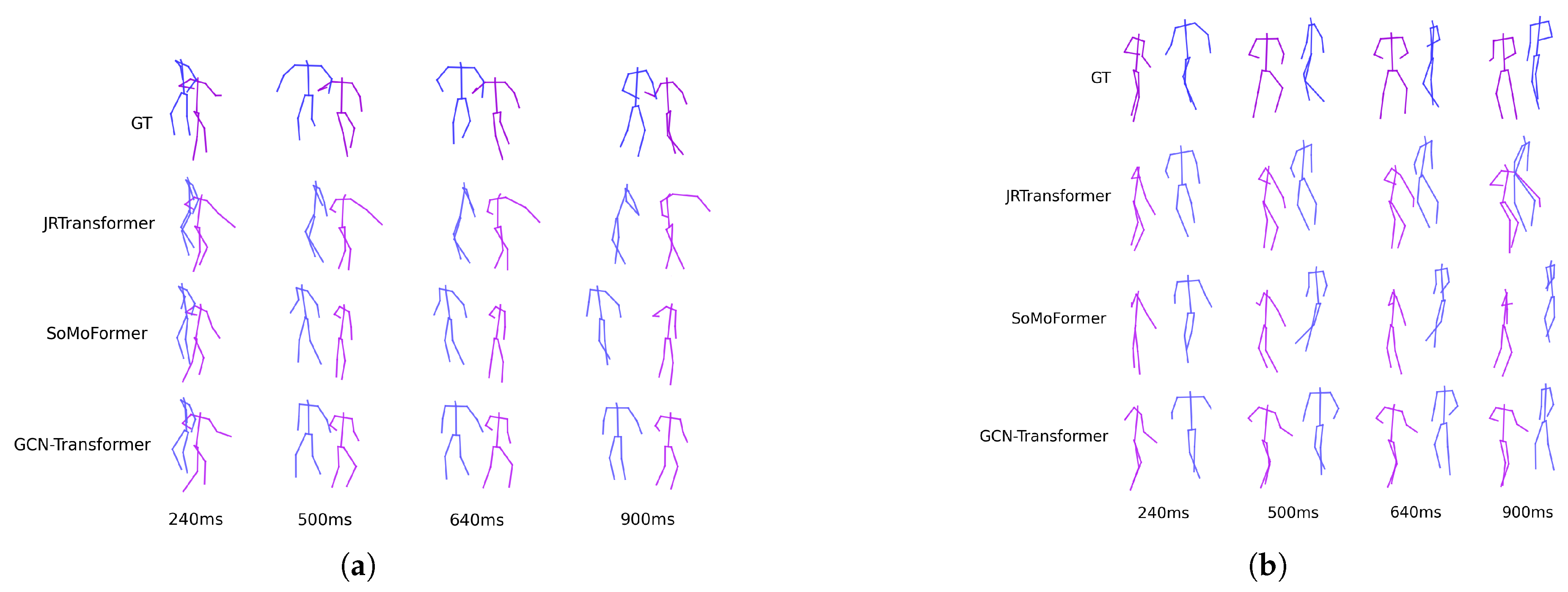
Figure 6.
The figure displays predicted poses on two example sequences from the ExPI test set for the top-performing models: JRTransformer, SoMoFormer, and GCN-Transformer, with GT indicating the ground truth. The sequence (a) shows one person jumping off the shoulders of another, while the sequence (b) shows one person performing a cartwheel assisted by another. The comparison illustrates that JRTransformer and SoMoFormer struggle with generating valid movements, often repeating the last known pose. In contrast, the GCN-Transformer demonstrates its capability to create realistic and dynamic movements.
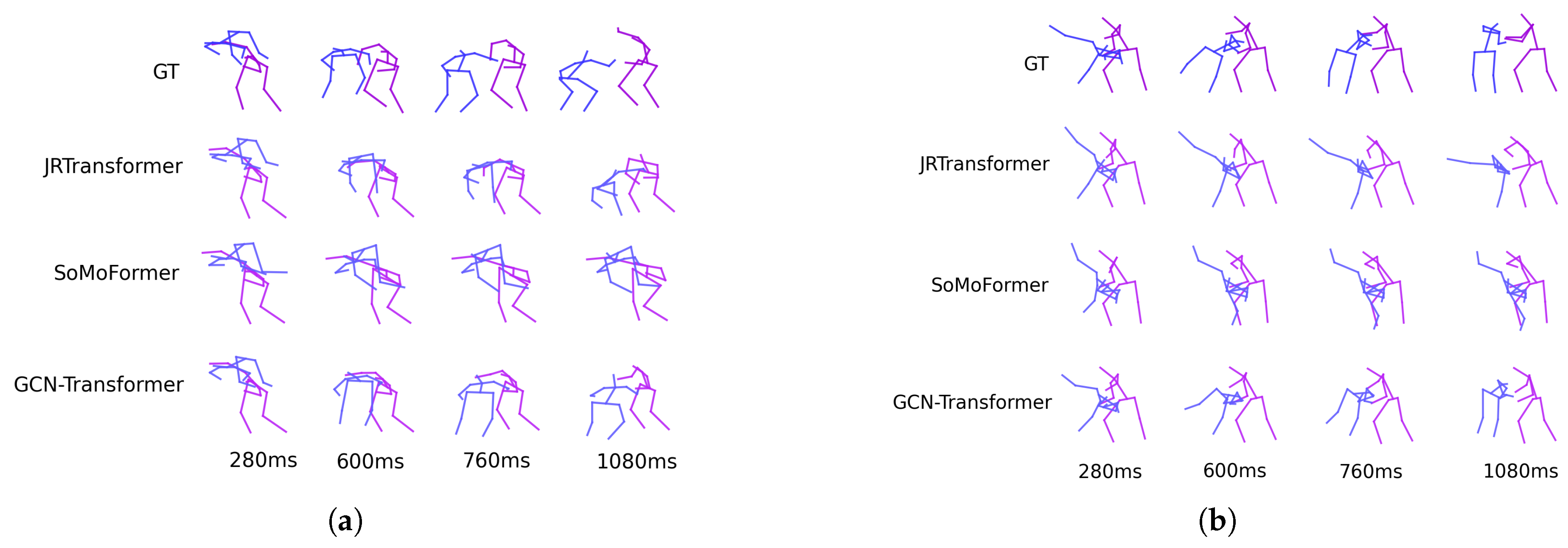
Figure 7.
The figure illustrates an example of predicted (purple) and ground truth (blue) joint trajectories, where T represents the time interval, and the values between the trajectories indicate their distances at time T. When the trajectories are identical but with a slight offset, FJPTE yields the same results as MPJPE and VIM. However, when the trajectories diverge, the metrics produce significantly different results. MPJPE and FJPTE evaluate full joint trajectory, while VIM evaluates only the last time interval .
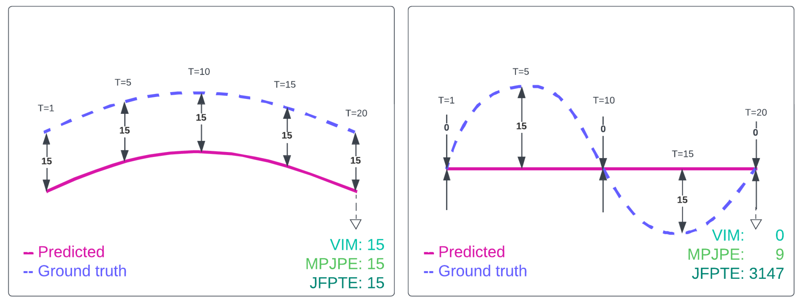
Figure 8.
The figure illustrates an example of predicted (purple) and ground truth (blue) sequences of poses, with T representing the time interval. The predicted sequence demonstrates a scenario where the global position aligns well with the ground truth, but the pose remains frozen or ghost-like, floating through space, a common issue in pose forecasting. Metrics like MPJPE and VIM evaluate joint distances independently across time intervals, while FJPTE goes further by assessing joint trajectories, distinguishing between local (FJPTElocal) and global (FJPTEglobal) movement. MPJPE and FJPTE evaluate the entire sequence, whereas VIM focuses only on the final time interval at .
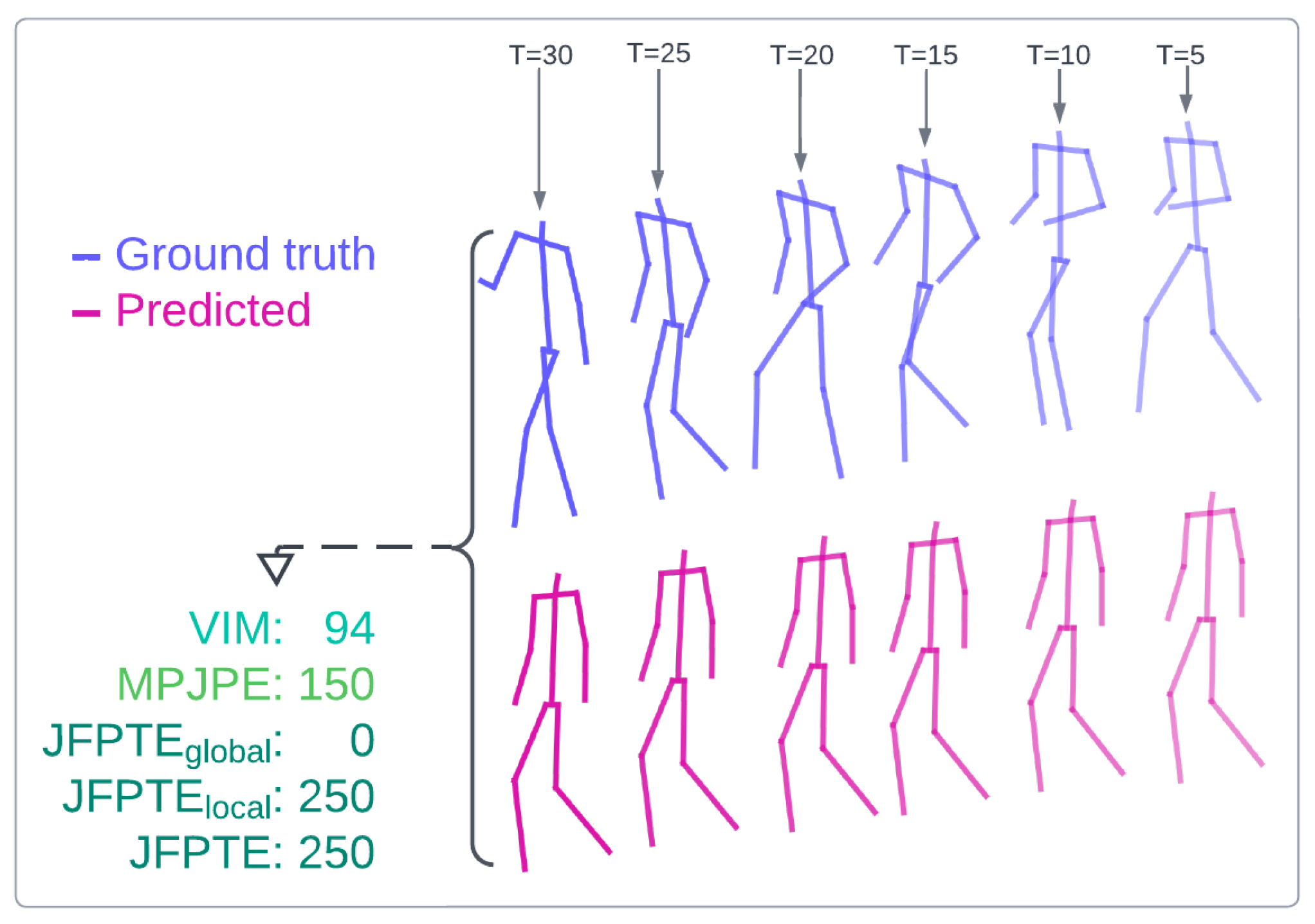
Figure 9.
Examples from the SoMoF (a) and ExPI (b) dataset illustrating the limitations of GCN-Transformer and other models in forecasting movements not observed during training. In the SoMoF sequence (a), one individual approaches another, initiating a complex movement where the two prepare to spin around each other in a dance-like motion. In the ExPI sequence (b), two individuals perform a complex action where one lifts the other overhead to execute a backflip. Due to the absence of such intricate interactions in the training data, the models struggle to predict the dynamic sequences and instead produce a static forecast, merely repeating the last observed poses of the individuals, failing to capture the expected motion.
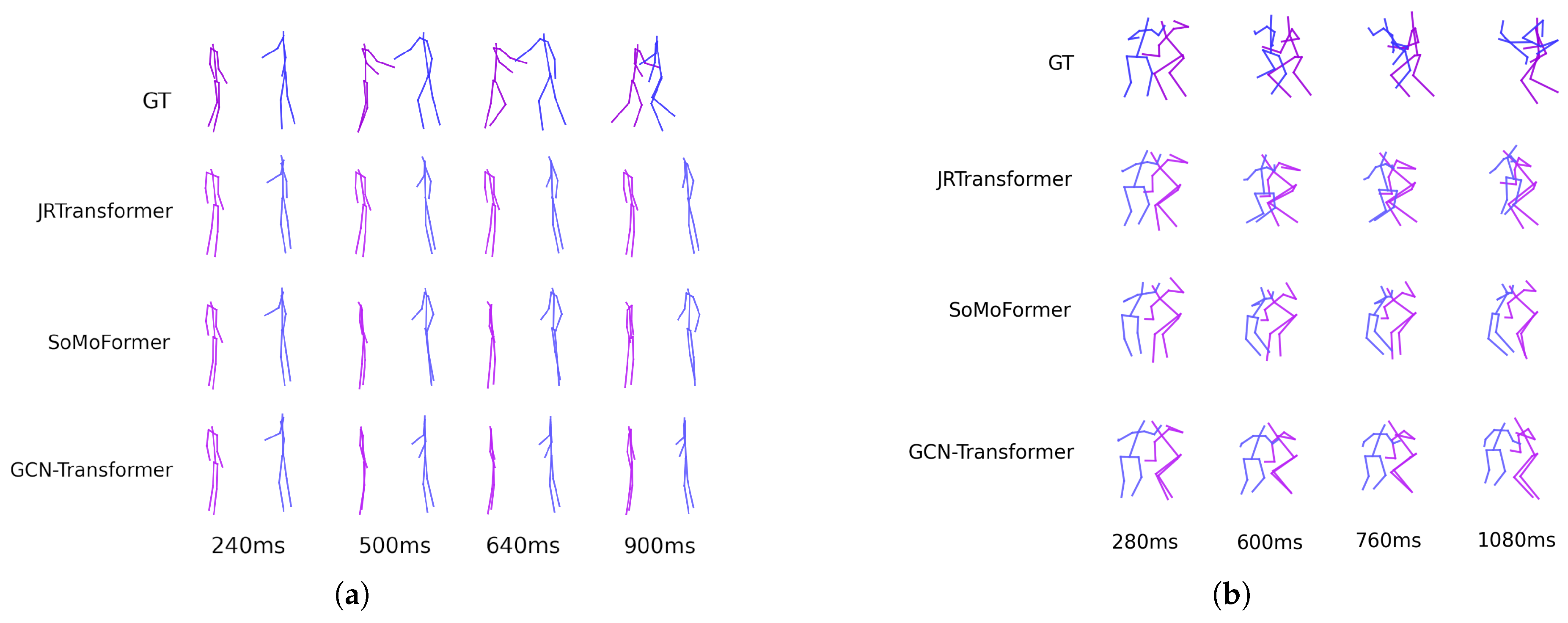

Table 1.
Performance comparison on the SoMoF Benchmark test set using the VIM and MPJPE metrics, where lower values indicate better performance. Our proposed model, GCN-Transformer, achieves state-of-the-art results. The model marked with an asterisk (*) incorporated the validation dataset during training and currently leads the official SoMoF Benchmark leaderboard at https://somof.stanford.edu.
| Method | VIM | MPJPE | ||||||||||
|---|---|---|---|---|---|---|---|---|---|---|---|---|
| 100ms | 240ms | 500ms | 640ms | 900ms | Overall | 100ms | 240ms | 500ms | 640ms | 900ms | Overall | |
| Zero Velocity | 29.35 | 53.56 | 94.52 | 112.68 | 143.10 | 86.65 | 55.28 | 87.98 | 146.10 | 173.30 | 223.16 | 137.16 |
| DViTA [9] | 17.40 | 35.62 | 72.06 | 90.87 | 127.27 | 68.65 | 32.09 | 54.48 | 100.03 | 124.07 | 173.01 | 96.74 |
| LTD [3] | 18.07 | 34.88 | 68.16 | 85.07 | 116.83 | 64.60 | 33.57 | 55.21 | 97.57 | 119.58 | 163.69 | 93.92 |
| TBIformer [16] | 17.62 | 34.67 | 67.50 | 84.01 | 116.38 | 64.03 | 32.26 | 53.65 | 95.61 | 117.22 | 160.99 | 91.94 |
| MRT [12] | 15.31 | 31.23 | 63.16 | 79.61 | 111.86 | 60.24 | 27.97 | 47.64 | 87.87 | 108.93 | 151.96 | 84.88 |
| SocialTGCN [17] | 12.84 | 27.41 | 58.12 | 74.59 | 107.19 | 56.03 | 23.10 | 40.24 | 76.91 | 96.89 | 139.01 | 75.23 |
| JRTransformer [15] | 11.17 | 25.73 | 56.50 | 73.19 | 106.87 | 54.69 | 18.44 | 35.38 | 72.26 | 92.42 | 135.12 | 70.73 |
| MPFSIR [14] | 11.57 | 25.37 | 54.04 | 69.65 | 101.13 | 52.35 | 20.31 | 35.69 | 69.58 | 88.36 | 128.37 | 68.46 |
| Future Motion [10] | 10.76 | 24.52 | 54.14 | 69.58 | 100.81 | 51.96 | 18.66 | 34.38 | 69.76 | 88.91 | 129.18 | 68.18 |
| SoMoFormer [13] | 10.45 | 23.10 | 49.76 | 64.30 | 93.34 | 48.19 | 17.63 | 32.42 | 63.86 | 81.20 | 117.97 | 62.62 |
| GCN-Transformer | 10.14 | 22.54 | 48.81 | 63.67 | 94.94 | 48.02 | 17.11 | 31.48 | 62.62 | 80.14 | 118.14 | 61.90 |
| GCN-Transformer* | 9.82 | 21.80 | 46.61 | 60.88 | 91.95 | 46.21 | 16.41 | 30.36 | 60.31 | 76.94 | 113.36 | 59.48 |
Table 2.
Performance comparison on the ExPI test set using the VIM and MPJPE metrics, where lower values indicate better performance. Our proposed model, GCN-Transformer, achieves state-of-the-art results on both metrics.
Table 2.
Performance comparison on the ExPI test set using the VIM and MPJPE metrics, where lower values indicate better performance. Our proposed model, GCN-Transformer, achieves state-of-the-art results on both metrics.
| Method | VIM | MPJPE | ||||||||||
|---|---|---|---|---|---|---|---|---|---|---|---|---|
| 120ms | 280ms | 600ms | 760ms | 1080ms | Overall | 120ms | 280ms | 600ms | 760ms | 1080ms | Overall | |
| Zero Velocity | 25.61 | 48.66 | 84.39 | 97.41 | 118.10 | 74.84 | 46.16 | 74.66 | 124.32 | 145.22 | 181.33 | 114.34 |
| DViTA [9] | 15.44 | 35.27 | 74.43 | 91.44 | 119.51 | 67.22 | 28.31 | 51.63 | 100.85 | 124.49 | 167.98 | 94.65 |
| LTD [3] | 16.22 | 32.94 | 62.73 | 74.60 | 92.84 | 55.87 | 28.83 | 48.73 | 87.37 | 104.82 | 135.61 | 81.07 |
| TBIformer [16] | 16.96 | 35.09 | 67.95 | 81.22 | 103.02 | 60.85 | 30.59 | 52.55 | 95.63 | 115.19 | 150.33 | 88.86 |
| MRT [12] | 15.32 | 32.07 | 61.84 | 74.04 | 94.59 | 55.57 | 27.79 | 47.91 | 87.01 | 104.80 | 137.22 | 80.95 |
| SocialTGCN [17] | 16.79 | 32.71 | 62.61 | 75.24 | 99.15 | 57.30 | 31.14 | 50.58 | 89.18 | 106.95 | 140.68 | 83.71 |
| JRTransformer [15] | 8.40 | 21.14 | 46.20 | 57.63 | 76.94 | 42.06 | 13.57 | 28.01 | 58.47 | 73.27 | 101.04 | 54.87 |
| MPFSIR [14] | 9.15 | 23.05 | 52.31 | 65.49 | 92.46 | 48.49 | 15.56 | 30.55 | 64.84 | 81.81 | 114.94 | 61.54 |
| Future Motion [10] | 16.94 | 34.83 | 68.45 | 83.33 | 108.03 | 62.32 | 30.51 | 52.37 | 96.06 | 116.88 | 156.04 | 90.37 |
| SoMoFormer [13] | 9.43 | 23.88 | 54.78 | 68.71 | 92.38 | 49.84 | 15.22 | 31.08 | 67.33 | 85.37 | 119.37 | 63.67 |
| GCN-Transformer | 8.32 | 20.84 | 44.56 | 54.81 | 74.66 | 40.64 | 13.37 | 27.63 | 57.27 | 71.25 | 97.71 | 53.45 |
Table 3.
The ablation study results are derived from the SoMoF Benchmark validation set and presented in VIM (top) and MPJPE (bottom) metrics. The baseline model comprises Scene Module and Spatio-Temporal Transformer Decoder, with subsequent additions incrementally incorporated into the model. All models are trained solely on the SoMoF Benchmark training dataset, excluding AMASS.
| Method | 100ms | 240ms | 500ms | 640ms | 900ms | Overall |
|---|---|---|---|---|---|---|
| Baseline | 15.39 | 28.53 | 55.90 | 68.72 | 93.92 | 52.49 |
| + Temporal-GCN | 12.69 | 28.96 | 58.96 | 69.74 | 89.56 | 51.98 |
| + MPJD loss | 11.08 | 28.80 | 57.52 | 67.55 | 87.95 | 50.58 |
| + Velocity loss | 12.21 | 28.30 | 56.12 | 66.42 | 87.67 | 50.14 |
| + Augmentation | 7.56 | 19.66 | 44.72 | 56.08 | 75.12 | 40.63 |
| Baseline | 31.81 | 45.19 | 77.03 | 93.68 | 127.60 | 75.06 |
| + Temporal-GCN | 23.99 | 41.47 | 79.33 | 96.38 | 127.61 | 73.76 |
| + MPJD loss | 18.09 | 37.54 | 76.08 | 92.69 | 123.51 | 69.58 |
| + Velocity loss | 22.79 | 39.90 | 75.28 | 91.15 | 121.77 | 70.18 |
| + Augmentation | 11.68 | 24.35 | 53.50 | 68.34 | 96.97 | 50.97 |
Table 4.
Comparison of performance on the SoMoF Benchmark test set using the proposed FJPTE metric, with lower values indicating superior performance. The table distinguishes between FJPTElocal and FJPTEglobal errors, with FJPTElocal representing movement dynamics error and FJPTEglobal measuring global position and trajectory error. The asterisk (*) denotes the model that integrated the validation dataset during training.
| Method | FJPTElocal | FJPTEglobal | ||||||||||
|---|---|---|---|---|---|---|---|---|---|---|---|---|
| 100ms | 240ms | 500ms | 640ms | 900ms | Overall | 100ms | 240ms | 500ms | 640ms | 900ms | Overall | |
| Zero Velocity | 65.36 | 97.18 | 142.35 | 158.79 | 178.72 | 128.48 | 91.12 | 146.51 | 241.69 | 284.08 | 363.52 | 225.38 |
| DViTA [9] | 55.15 | 91.84 | 147.91 | 168.07 | 194.29 | 131.45 | 47.60 | 81.35 | 162.46 | 212.71 | 319.11 | 164.65 |
| LTD [3] | 48.96 | 78.96 | 127.59 | 145.98 | 170.41 | 114.38 | 52.86 | 88.66 | 159.64 | 201.40 | 290.96 | 158.70 |
| TBIformer [16] | 55.24 | 88.28 | 138.76 | 156.81 | 178.97 | 123.61 | 51.19 | 84.53 | 150.47 | 190.78 | 283.36 | 152.07 |
| MRT [12] | 56.38 | 90.59 | 143.17 | 162.19 | 186.11 | 127.69 | 46.74 | 77.70 | 147.95 | 189.65 | 279.84 | 148.37 |
| SocialTGCN [17] | 51.50 | 83.54 | 137.45 | 157.54 | 183.19 | 122.64 | 39.76 | 65.92 | 132.28 | 175.90 | 271.09 | 136.99 |
| JRTransformer [15] | 41.20 | 72.47 | 124.75 | 145.87 | 174.81 | 111.82 | 26.87 | 54.81 | 122.92 | 166.64 | 264.94 | 127.24 |
| MPFSIR [14] | 43.53 | 75.36 | 127.59 | 148.60 | 180.67 | 115.15 | 27.37 | 51.27 | 109.84 | 151.17 | 248.05 | 117.54 |
| Future Motion [10] | 42.74 | 72.22 | 122.18 | 140.77 | 165.83 | 108.75 | 31.04 | 54.72 | 117.86 | 158.93 | 249.45 | 122.40 |
| SoMoFormer [13] | 37.69 | 65.48 | 111.48 | 128.79 | 154.44 | 99.58 | 26.13 | 48.37 | 104.01 | 139.66 | 217.92 | 107.22 |
| GCN-Transformer | 37.22 | 63.78 | 109.06 | 126.12 | 152.72 | 97.78 | 24.35 | 47.42 | 107.12 | 146.38 | 234.51 | 111.96 |
| GCN-Transformer* | 36.76 | 62.29 | 104.96 | 121.68 | 147.97 | 94.73 | 23.63 | 45.89 | 102.05 | 138.45 | 228.94 | 107.79 |
Table 5.
Comparison of performance on the ExPI test set using the proposed FJPTE metric, with lower values indicating superior performance. The table distinguishes between FJPTElocal and FJPTEglobal errors, with FJPTElocal representing movement dynamics error and FJPTEglobal measuring global position and trajectory error.
| Method | FJPTElocal | FJPTEglobal | ||||||||||
|---|---|---|---|---|---|---|---|---|---|---|---|---|
| 120ms | 280ms | 600ms | 760ms | 1080ms | Overall | 120ms | 280ms | 600ms | 760ms | 1080ms | Overall | |
| Zero Velocity | 76.63 | 119.52 | 182.09 | 205.19 | 240.31 | 164.75 | 79.80 | 127.56 | 201.88 | 230.77 | 280.05 | 184.01 |
| DViTA [9] | 56.91 | 101.25 | 176.21 | 206.20 | 252.27 | 158.57 | 45.58 | 83.58 | 164.19 | 202.36 | 271.01 | 153.34 |
| LTD [3] | 60.27 | 97.73 | 159.16 | 182.82 | 217.66 | 143.53 | 47.42 | 80.89 | 141.84 | 169.41 | 215.70 | 131.05 |
| TBIformer [16] | 67.38 | 109.04 | 174.85 | 200.29 | 239.29 | 158.17 | 50.23 | 86.97 | 155.57 | 184.96 | 238.15 | 143.18 |
| MRT [12] | 65.77 | 107.77 | 173.87 | 199.12 | 236.71 | 156.65 | 43.80 | 75.45 | 133.75 | 162.58 | 214.24 | 125.96 |
| SocialTGCN [17] | 72.62 | 110.05 | 174.62 | 201.84 | 247.24 | 161.27 | 52.04 | 83.27 | 149.11 | 178.12 | 237.98 | 140.10 |
| JRTransformer [15] | 37.98 | 71.62 | 130.94 | 155.35 | 197.44 | 118.67 | 26.21 | 52.63 | 102.44 | 126.11 | 168.75 | 95.23 |
| MPFSIR [14] | 41.12 | 77.88 | 145.78 | 174.01 | 225.03 | 132.76 | 27.21 | 54.68 | 112.28 | 140.63 | 207.33 | 108.43 |
| Future Motion [10] | 64.87 | 105.26 | 175.12 | 206.69 | 247.48 | 159.88 | 48.70 | 86.51 | 160.21 | 197.70 | 270.41 | 152.71 |
| SoMoFormer [13] | 41.91 | 80.52 | 150.92 | 179.58 | 224.17 | 135.42 | 28.82 | 57.92 | 118.39 | 148.45 | 204.18 | 111.55 |
| GCN-Transformer | 38.39 | 71.60 | 125.41 | 146.24 | 181.17 | 112.56 | 26.67 | 52.74 | 100.23 | 122.83 | 172.73 | 95.04 |
Table 6.
Comparison of performance on the SoMoF Benchmark test set (left) and the ExPI test set (right) using the proposed FJPTE metric, where lower values indicate better performance. The table presents FJPTE metrics, combining FJPTElocal and FJPTEglobal errors for a comprehensive performance evaluation. Our model achieves state-of-the-art results on the FJPTE metric. The asterisk (*) indicates models that integrated the validation dataset during training.
| Method | SoMoF Benchmark | ExPI | ||||||||||
|---|---|---|---|---|---|---|---|---|---|---|---|---|
| 100ms | 240ms | 500ms | 640ms | 900ms | Overall | 120ms | 280ms | 600ms | 760ms | 1080ms | Overall | |
| Zero Velocity | 156.48 | 243.69 | 384.04 | 442.87 | 542.24 | 353.86 | 156.43 | 247.07 | 383.97 | 435.95 | 520.36 | 348.76 |
| DViTA [9] | 102.75 | 173.20 | 310.36 | 380.78 | 513.40 | 296.10 | 102.48 | 184.82 | 340.40 | 408.56 | 523.29 | 311.91 |
| LTD [3] | 101.82 | 167.62 | 287.23 | 347.38 | 461.37 | 273.08 | 107.69 | 178.62 | 301.01 | 352.23 | 433.36 | 274.58 |
| TBIformer [16] | 106.43 | 172.81 | 289.23 | 347.59 | 462.33 | 275.68 | 117.61 | 196.01 | 330.42 | 385.25 | 477.45 | 301.35 |
| MRT [12] | 103.11 | 168.29 | 291.12 | 351.84 | 465.95 | 276.06 | 109.58 | 183.22 | 307.63 | 361.70 | 450.95 | 282.62 |
| SocialTGCN [17] | 91.26 | 149.46 | 269.73 | 333.44 | 454.28 | 259.63 | 124.66 | 193.32 | 323.73 | 379.95 | 485.22 | 301.38 |
| JRTransformer [15] | 68.07 | 127.29 | 247.68 | 312.51 | 439.75 | 239.06 | 64.19 | 124.25 | 233.39 | 281.46 | 366.19 | 213.90 |
| MPFSIR [14] | 70.91 | 126.63 | 237.44 | 299.78 | 428.72 | 232.69 | 68.33 | 132.56 | 258.06 | 314.65 | 432.35 | 241.19 |
| Future Motion [10] | 73.78 | 126.94 | 240.04 | 299.70 | 415.28 | 231.15 | 113.57 | 191.77 | 335.33 | 404.39 | 517.89 | 312.59 |
| SoMoFormer [13] | 63.82 | 113.85 | 215.50 | 268.45 | 372.35 | 206.79 | 70.73 | 138.44 | 269.31 | 328.03 | 428.35 | 246.97 |
| GCN-Transformer | 61.57 | 111.21 | 216.17 | 272.50 | 387.22 | 209.73 | 65.07 | 124.34 | 225.64 | 269.07 | 353.90 | 207.60 |
| GCN-Transformer* | 60.39 | 108.19 | 207.01 | 260.13 | 376.91 | 202.53 | - | - | - | - | - | - |
Disclaimer/Publisher’s Note: The statements, opinions and data contained in all publications are solely those of the individual author(s) and contributor(s) and not of MDPI and/or the editor(s). MDPI and/or the editor(s) disclaim responsibility for any injury to people or property resulting from any ideas, methods, instructions or products referred to in the content. |
© 2025 by the authors. Licensee MDPI, Basel, Switzerland. This article is an open access article distributed under the terms and conditions of the Creative Commons Attribution (CC BY) license (http://creativecommons.org/licenses/by/4.0/).
Copyright: This open access article is published under a Creative Commons CC BY 4.0 license, which permit the free download, distribution, and reuse, provided that the author and preprint are cited in any reuse.


